Excitations of strange bottom baryons

Abstract

The ground state and first excited state masses of $\Omega_{b}$ and $\Omega_{bb}$ baryons are calculated in lattice QCD using dynamical $2+1$ flavour gauge fields. A set of baryon operators employing different combinations of smeared quark fields was used in the framework of the variational method. Results for radial excitation energies were confirmed by carrying out a supplementary multiexponential fitting analysis. Comparison is made with quark model calculations.

I Introduction

The calculation of hadronic excitation energies is an important area of activity for lattice QCD. Hadrons containing both heavy and light quarks present an interesting challenge since one has to deal with quarks at many different mass scales. Recently results for radial excitations of heavy-light hadrons were reviewed Woloshyn:2016cgd and it was found that in the meson sector there was reasonably good agreement between lattice QCD simulations, quark models and available (but still incomplete) experimental data. However, for baryons containing a single charm or bottom quark there seems to be a puzzle. The few results obtained for radial excitations of S-wave singly heavy baryons are consistently larger than quark model values. Whereas the quark model suggests that excitation energies of heavy-light baryons should be smaller than that of heavy-light mesons the lattice results reviewed in Woloshyn:2016cgd do not show this qualitative feature. Unfortunately, experiment is unlikely to settle this issue any time soon.

In addition to predicting that baryonic excitations are smaller than mesonic ones, quark models also predict that the lowest lying radial excitation of a doubly heavy baryon should be significantly smaller than of a singly heavy baryon (see, for example, fig. 3 in Roberts:2007ni ). This is due to the different excitation modes at play Roberts:2007ni ; Ebert:2002ig ; Yoshida:2015tia . In a singly heavy baryon the lowest lying excitation is due to the motion of the heavy quark relative to the diquark system formed by the light quarks. In a doubly heavy baryon it is the excitation of the heavy quark pair that is important. This effect is particularly pronounced for bottom baryons. It is natural to ask if the features of the spectrum which these quark model mechanisms predict are reproduced in a lattice QCD simulation. This is the theme of the present paper.

In this work we focus on the lattice simulation of spin $\nicefrac{{1}}{{2}}$ baryons $\Omega_{b}$ and $\Omega_{bb}.$ Since the valence quark content of these baryons consists only of strange and bottom the values of the $u$ and $d$ sea quark masses are of secondary importance. For our simulation the $u$ and $d$ quarks are near physical corresponding to a pion mass of $156(7)MeV$ so $u,d$ mass extrapolation is not carried out. Secondly, with strange quark valence content statistical fluctuations are considerably smaller than what would have been possible if $u,d$ valence quarks would have been used.

The lattice setup for the present work is described in sect. II. In sect. III the analysis method and results are presented. The results are compared to a number of recent quark model calculations. A summary is given in sect. IV.

II Lattice setup

The $2+1$ dynamical flavour gauge field configurations used in this work were generated by the PACS-CS Collaboration pacscs09 on a $32^{4}\times 64$ lattice using the Iwasaki action ($\beta=1.90$) for the gauge field and the clover-Wilson action for the fermions. The strange quark hopping parameter used here was $0.13666$ which is slightly different than that used by the PACS-CS Collaboration and is in line with the value determined from earlier work on the $D_{s}$ spectrum Lang:2014yfa . The strange quark clover coefficient was $1.715$. The gauge field ensemble had 198 configurations. For this ensemble PACS-CS determined a lattice spacing of $a=0.0907(13)fm$.

The bottom quark was described using tadpole-improved lattice NRQCD Lepage:1992 . The Hamiltonian is the same as used in previous calculation of bottom baryon masses and may be found in the Appendix of ref. Lewis:2009 Terms up to order $v^{4}$ were retained in the nonrelativistic expansion. The $b$-quark bare mass was $1.945$ as determined in ref. Lewis:2011 from tuning to S-wave bottomonium. The average link in Landau gauge, estimated to be $0.8463$, was used for tadpole improvement and the stability parameter $n$ appearing in the NRQCD Hamiltionian was taken to be 4. As a check of the lattice NRQCD setup the $\Upsilon$ - $\eta_{b}$ mass difference was calculated with the result $58.1(1.5)MeV$ in excellent agreement with the experimental value $57.9(2.4)MeV$ obtained using the PDG pdg value for the $\Upsilon$ mass and the Belle result Belle:2012 for $\eta_{b}$.

The baryon operators used in our calculation take the form

$$\epsilon^{abc}[q_{a}^{T}C\gamma_{5}q^{\prime}_{b}]q_{c}$$ (1)

where for the spin $\nicefrac{{1}}{{2}}$ $\Omega_{b}$ baryon $q$ is a strange quark field and $q^{\prime}$ is bottom. For $\Omega_{bb}$, $q$ is a bottom quark field and $q^{\prime}$ is strange.

The simplest operator that one can construct of the form (1) has all quark fields at the same space-time point. However to disentangle ground and excited state contributions to correlation functions it is advantageous to use a variety of spatially smeared operators which will lead to different admixtures of states in the correlators. Successful phenomenological descriptions of baryons are often made using a quark-diquark model which implies strong spatial correlations among the constituents. Ideally, we would like to construct lattice baryon operators incorporating quark-quark correlations. However a usable scheme for doing this is not available so here independent spatial smearing of the quark fields is carried out.

Quark fields are smeared according to

$$\tilde{\psi}({\bf x})=\sum_{\bf y}f({\bf x}-{\bf y})\,\psi({\bf y})$$ (2)

where f is a gauge field independent profile function. Since this is not gauge covariant a gauge fixing to Coulomb gauge is carried out on the gauge field links prior to use. A choice for the profile $f$ which has been used successfully in NRQCD applications is motivated by the shape of wavefunctions for the Coulomb potential Gray:2005 ; Davies:2010 . In this work we use mostly a smearing function of the form $e^{-\frac{r}{a_{0}}}$ where $r$ is the shortest distance between ${\bf y}$ and ${\bf x}$ in a periodic box. This will be referred to as ground state smearing. An excited state smearing function $(a_{n}-r)e^{-\frac{r}{a_{1}}})$ was also considered. Since excited state smearing tends to lead to noisier correlators this smearing was used only in a supplementary calculation.

The strange quark field was given a more spatially extended profile than the bottom quark. After some trials the smearing parameters (in lattice units) chosen for this work were $a_{0}=1.6,a_{1}=3.2,a_{n}=3.17$ for the bottom quark and $a_{0}=3.0,a_{1}=5.5,a_{n}=7.0$ for strange.

III Analysis and results

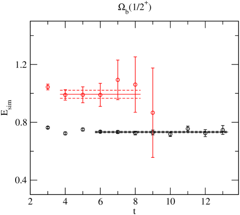
Figure 1: Effective simulation energies in lattice units for the ground and first excited state of $\Omega_{b}$. The horizontal lines indicate the fit value and time range used.

Lattice Euclidean-time correlation functions are typically dominated by the ground state after a fairly small number of time steps. To extract excited state information requires some work. The approach used here is the so-called variational method Luscher:1990 ; Michael:1985 ; Blossier:2009 . A set of basis operators $\{O\}$ is chosen and one constructs the correlator matrix

$$C_{ij}(t=t_{f}-t_{i})=\langle 0|O_{i}(t_{f})O_{j}^{\dagger}(t_{i})|0\rangle$$ (3)

where $t_{i}$ and $t_{f}$ denote the source and sink times. The generalized eigenvalue problem Blossier:2009 is solved for each time step larger than some reference time $t_{0}$

$$C(t)\vec{w}^{(k)}=\lambda^{(k)}(t)C(t_{0})\vec{w}^{(k)}.$$ (4)

Energies are extracted from the time dependence of the eigenvalues $\lambda$ and for a well chosen basis and $t_{0}$ the eigenvalues of the lowest lying states are dominated by a single exponential function.

For the main calculation a set of six operators with different combinations of unsmeared ($p$) and ground state smeared ($g$) fields is used. The operators are denoted as

$$ppp,ppg,gpg,pgp,pgg,ggg$$ (5)

where the first and third letters indicate the smearing level of $q$ fields in eq. (1) (strange for $\Omega_{b}$, bottom for $\Omega_{bb}$) and the second letter indicates the smearing level of $q^{\prime}$ field (bottom for $\Omega_{b}$, strange for $\Omega_{bb}$). Note that for $\Omega_{b}$ energies of both positive and negative parity states can be extracted by choosing different components of the relativistic operator.

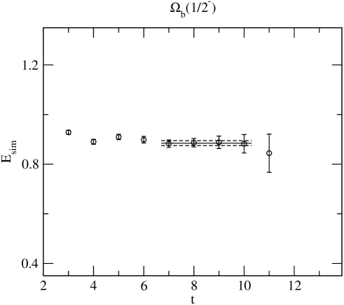
Figure 2: Effective simulation energies in lattice units for the ground state of the negative parity $\Omega_{b}$. The horizontal lines indicate the fit value and time range used.

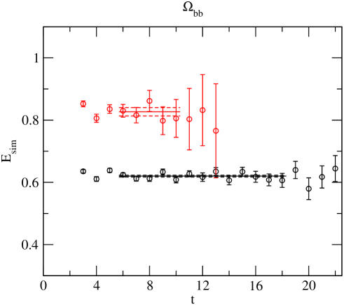
Figure 3: Effective simulation energies in lattice unitsfor the ground and first excited state of $\Omega_{b}$. The horizontal lines indicate the fit value and time range used.

For each configuration correlation functions were averaged over 16 different source time positions. The generalized eigenvalue problem (4) was solved using $t_{0}=2$. The effective simulation energies (lattice units) for the positive parity $\Omega_{b}$ extracted from the eigenvalues of the two lowest states are shown in fig. 1. The horizontal lines show the fitted simulation energy values along with time range used to determine them. The ground state is very well determined. The first excited state is well separated from the ground state and the energy can be extracted with a reasonably small statistical uncertainty. Figure 2 shows the ground state simulation energy for $\Omega_{b}({\nicefrac{{1}}{{2}}}^{-})$. In this case only the ground state is reasonably well determined.

The simulation energy results for $\Omega_{bb}$ are plotted in fig. 3. For $\Omega_{bb}$ only the positive parity state is available due to the nonrelativistic treatment of the bottom quark.

Table 1: Extracted simulation energies in lattice units for the variational and multiexponential fitting methods.

State	Variational	Multiexponential
$\Omega_{b}({\nicefrac{{1}}{{2}}}^{+})$ g.s.	0.7324(50)(24)	0.7262(43)
$\Omega_{b}({\nicefrac{{1}}{{2}}}^{+})$ excited	0.9938(278)(10)	0.9904(329)
$\Omega_{b}({\nicefrac{{1}}{{2}}}^{-})$ g.s.	0.8847(99)(90)	0.8801(44)
$\Omega_{bb}({\nicefrac{{1}}{{2}}}^{+})$ g.s.	0.6201(29)(20)	0.6137(22)
$\Omega_{bb}({\nicefrac{{1}}{{2}}}^{+})$ excited	0.8267(133)(24)	0.8015(139)

The values for the fitted simulation energies are given in table 1. The first error is statistical, the second is an estimate of the uncertainty due to different choices of time range to include in the fit.

To provide additional confirmation that our extraction of excited state energies is reliable a second analysis was done using a different method and a different set of correlation functions. Since smearing at the sink usually leads to noisier correlators than smearing at the source a set of correlation function was constructed with source operators using combinations of fields

$$gpg,gpe,epe,ggg,ege$$ (6)

where $e$ denotes smearing with an excited state profile and a local operator $ppp$ at the sink. A simultaneous constrained multiexponential fit Lepage:2001ym to the five correlation functions was done using four terms. As in the variational analysis correlation functions were averaged over a set of sixteen different time sources for each gauge configuration. The correlation functions and fits are shown in fig. 4 to fig. 6. The time range used for fitting was 2 to 18 for $\Omega_{b}$ and 3 to 20 for $\Omega_{bb}$. The source corresponds to $t=1$. The simulation energies for the ground and first excited states are given in table 1. They are compatible within statistical errors with the results obtained using the correlator matrix variational method.

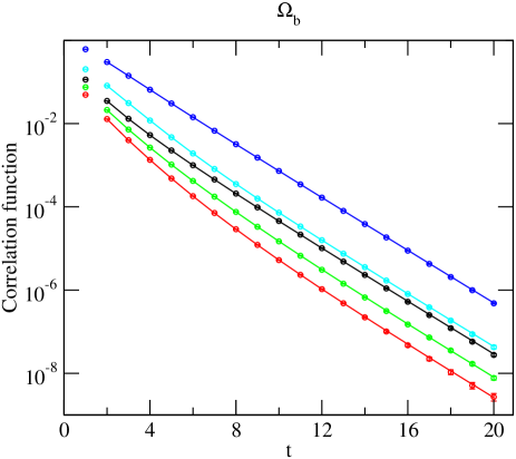
Figure 4: Correlation functions for the positive parity $\Omega_{b}$ along with the result of a simultaneous four-term multiexponential fit.

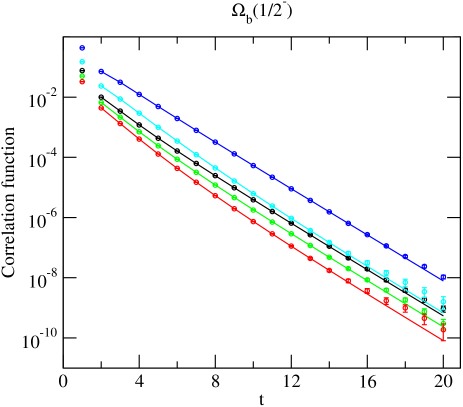
Figure 5: Correlation functions for the negative parity $\Omega_{b}$ along with the result of a simultaneous four-term multiexponential fit.

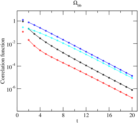
Figure 6: Correlation functions for the $\Omega_{bb}$ along with the result of a simultaneous four-term multiexponential fit. Due to the node in the excited state profile file function the correlator with source smearing $gpe$ has a negative piece and is omitted from the plot.

Since quark mass has been removed from the lattice NRQCD Hamiltonian the simulation energies extracted from the correlation do not give the hadron mass directly. However, differences between simulation energies in lattice units are related to mass differences by the inverse of the lattice spacing. Our calculated mass differences ${\Delta}M$ between the first radial excitation and the ground state for $\Omega_{b}$ and for $\Omega_{bb}$ are given in table 2. The three errors shown for this work are the statistical error and uncertainties due to fitting time range and the lattice spacing determination. Table 2 also shows the calculated mass difference between the positive and negative parity ground states of $\Omega_{b}$. For comparison we note that an earlier lattice study Woloshyn:2016cgd gave mass differences for $\Lambda_{b}$ and $\Sigma_{b}$ of $344(105)MeV$ and $252(60)MeV$ respectively. The PGD value for the $\Lambda_{b}({\nicefrac{{1}}{{2}}}^{-})-\Lambda_{b}({\nicefrac{{1}}{{2}}}^{+})$ mass difference is $293(1)MeV$.

Table 2: Mass differences and masses in MeV from this work and some recent quark model calculations. The errors associated to this work are due to statistics, fitting and scale setting

	This work	ref. Roberts:2007ni	ref. Ebert:2002ig ; Ebert:2011kk	ref. Yoshida:2015tia	ref. Garcilazo:2007eh
${\Delta}M(\Omega_{b})$	$569(61)(6)(8)$	$391$	$386$	$441$	$330$
${\Delta}M(\Omega_{bb})$	$450(29)(6)(6)$	$239$	$251$	$260$
$\Omega_{b}({\nicefrac{{1}}{{2}}}^{-})-\Omega_{b}({\nicefrac{{1}}{{2}}}^{+})$	$331(24)(19)(5)$	$220$	$275$	$257$	$241$
$M_{\Omega_{b}}$	$6038(11)(5)(18)$	$6081$	$6064$	$6076$	$6037$
$M_{\Omega_{bb}}$	$10238(6)(4)(11)$	$10454$	$10359$	$10447$

One way to get the baryon mass would be to calculate the kinetic energy as a function of momentum and determine a kinetic mass. However, this would be very time consuming and likely would have large statistical errors. Instead we use the fact the bottom quark bare mass was tuned by fitting the mass of bottomonium. The simulation energy of $\Upsilon$ can related to the mass by

$$M_{\Upsilon}=E_{sim}^{\Upsilon}+{\frac{1}{2}}(ZM_{0}-E_{shift}).$$ (7)

In (7) $M_{0}$ is the bottom bare mass, $Z$ is the mass renormalization factor and $E_{shift}$ is an additive mass shift that appears in lattice NRQCD Lepage:1992 . These quantities are independent of the hadron state so the combination appearing in the right hand side of (7) can be determined using the known $\Upsilon$ mass and the value of $E_{sim}^{\Upsilon}$ which is calculated to be $0.2624(7)$. Then

$$M_{\Omega_{b}}=E_{sim}^{\Omega_{b}}+{\frac{1}{2}}(M_{\Upsilon}-E_{sim}^{\Upsilon})$$ (8)

and

$$M_{\Omega_{bb}}=E_{sim}^{\Omega_{bb}}+M_{\Upsilon}-E_{sim}^{\Upsilon}.$$ (9)

The values obtained in this way are given in table 2. Note that the calculated value for the mass of the ground state of $\Omega_{b}$ is compatible with the experimental value pdg of $6048(3)MeV$.

In table 2 the results from several recent quark model calculations are also shown. The quark models have the feature that the energy of the lowest lying radial excitation of $\Omega_{bb}$ is significantly smaller than that of $\Omega_{b}$. This is due to different modes being excited as illustrated very nicely in ref. Roberts:2007ni for example. The lattice results also indicate a reduction of excitation energy in $\Omega_{bb}$ compared to $\Omega_{b}$ but not to the same level as the quark models. A similar effect is present in a lattice calculation done for charm baryons Bali:2015lka where, for example, radial excitation energies of $\Omega_{c}$ and $\Omega_{cc}$ were found to be $626(48)(53)MeV$ and $434(32)(33)MeV$ respectively. For comparison, the quark model of ref. Roberts:2007ni gives $434MeV$ for $\Omega_{c}$ and $365$ for $\Omega_{cc}$.

In this work, and in other lattice QCD studies where single-bottom baryon Woloshyn:2016cgd and heavy-light charm baryon Bali:2015lka ; Padmanath:2014bxa ; Padmanath:2015jea radial excitation energies were calculated, it is a consistent finding that lattice QCD yields excitation energies larger than quark models. In Woloshyn:2016cgd it is also pointed out that lattice QCD values for radial excitation energies of singly-heavy baryons are generally larger or comparable to the excitation energies of heavy-light mesons while quark model baryonic excitations are found to be smaller than those of mesons. It should also be noted that lattice QCD and quark models give reasonably compatible results for excitation energies of heavy-light mesons Woloshyn:2016cgd .

It is natural to ask if this work and other the lattice calculations done to date Woloshyn:2016cgd ; Bali:2015lka ; Padmanath:2014bxa ; Padmanath:2015jea indicate an irreconcilable difference with quark models for heavy-light baryon spectroscopy. It is probably premature to conclude this as there are still systematic effects that have not been studied systematically. Lattice calculations have been done in a variety of lattice setups for up and down quark masses, including the present work where there are no valance u,d quarks and the sea u,d quark masses are near physical. Since the qualitative comparison of lattice simulations with quark models is the same for all setups light quark mass extrapolation may not be a primary issue. Perhaps more significantly no continuum extrapolation was carried out in the lattice calculations mentioned above. It is tempting to point to this systematic as the source of all discrepancies. However, ground state mass values tend to be well described by these simulations so finite lattice spacing is not an obvious big issue.

The spatial lattice size used in the simulations discussed here ranges from $1.8$ to $2.9fm$. Only in Bali:2015lka was the lattice volume effect considered. For excited states, it was difficult to see the finite volume effect due to large statistical fluctuations. What we propose here is that differences seen between present lattice simulations and quark models for radial excitation energies may at the same time be pointing to the resolution of the issue. The lattice QCD discrepancy with quark models is seen to be larger for singly heavy baryons than for doubly heavy baryons. Since it is expected that singly heavy baryons are more strongly affected by finite volume effects this may be indicating the need for baryon simulations in larger spatial volumes.

IV Summary

Masses for spin ${\nicefrac{{1}}{{2}}}$ $\Omega_{b}$ and $\Omega_{bb}$ baryons were calculated using lattice QCD. As well, the energies of lowest lying radial excitations were computed. At present, there is no experimental information about radial excitations in heavy-light baryons so comparison is made to quark models. Quark models have the interesting feature that the radial excitation energies in doubly-heavy baryons are significantly smaller than for singly-heavy baryons. This is particularly evident for bottom baryons. This effect is seen in the present calculation but not to the extent predicted by quark models.

Summarizing the comparison of this work and a number of other lattice QCD calculations Woloshyn:2016cgd ; Bali:2015lka ; Padmanath:2014bxa ; Padmanath:2015jea for heavy-light baryons with quark model results one notes that excitation energies are consistently larger in the lattice calculations. This is particularly evident for charm baryons Bali:2015lka ; Padmanath:2014bxa . However, it is probably premature to conclude that lattice QCD and quark models predict very different heavy-light baryon spectroscopy since systematic effects in the lattice simulations still have not been explored fully. The largest discrepancy between lattice simulations and quark models occurs for single charm baryons (See ref. Woloshyn:2016cgd ) and decreases for double charm and bottom baryons. It is suggested that this pattern maybe due to finite lattice volume effects.

We hope that this work will provide motivation for further studies of heavy-light baryons to fill in the gaps in lattice QCD simulations and in experimental information.

We thank R. Lewis and D. Mohler for helpful comments and the PACS-CS Collaboration for making their dynamical gauge field configurations available. TRIUMF receives federal funding via a contribution agreement with the National Research Council of Canada.

References

- (1) R. M. Woloshyn and M. Wurtz, arXiv:1601.01925[hep-ph].
- (2) W. Roberts and M. Pervin, Int. J. Mod. Phys. A 23, 2817 (2008).
- (3) D. Ebert, R. N. Faustov, V. O. Galkin, and A. P. Martynenko, Phys. Rev. D 66, 014008 (2002).
- (4) T. Yoshida, E. Hiyama, A. Hosaka, M. Oka, and K. Sadato, Phys. Rev. D 92, 114029 (2015).
- (5) S. Aoki, et al. [PACS-CS Collaboration], Phys. Rev. D 79, 034503 (2009).
- (6) D. Mohler, C. B. Lang, L. Leskovec, S. Prelovsek, and R. M. Woloshyn, Phys. Rev. Lett. 111, 222001 (2013).
- (7) G. P. Lepage, L. Magnea, C. Nakhleh, U. Magnea, and K. Hornbostel, Phys. Rev. D 46, 4052 (1992).
- (8) R. Lewis and R. M. Woloshyn Phys. Rev. D 79, 014502 (2009).
- (9) R. Lewis and R. M. Woloshyn Phys. Rev. D 84, 094501 (2011).
- (10) K. A. Olive et al. (Particle Data Group), Chin. Phys. C 38, 090001 (2014).
- (11) R. Mizuk et al. (Belle Colaboration), Phys. Rev. Lett. 109, 232002 (2012).
- (12) A. Gray, I. Allison, C. T. H. Davies, E. Dalgic, G. P. Lepage, J. Shigemitsu, and M. Wingate, Phys. Rev. D 72, 094507 (2005).
- (13) C. T. H. Davies, E. Follana, I. D. Kendall, G. P. Lepage, and C. McNeile, Phys. Rev. D 81, 034506 (2010).
- (14) M. Lüscher and U. Wolff Nucl. Phys. B339, 222 (1990).
- (15) C. Michael, Nucl. Phys. B259, 58 (1990).
- (16) B. Blossier, M. Della Morte, G. von Hippel, T. Mendes, and R. Sommer, J. High Energy Phys. 04, 094 (2009).
- (17) G. P. Lepage, B. Clark, C. T. H. Davies, K. Hornbostel, P. B. Mackenzie, C. Morningstar, and H. Trottier, Nucl. Phys. Proc. Suppl. 106, 12 (2002).
- (18) D. Ebert, R. N. Faustov, and V. O. Galkin, Phys. Rev. D 84, 014025 (2011).
- (19) H. Garcilazo, T. Vijande, and A. Valcarce, J. Phys. G 34, 961 (2007).
- (20) P. Pérez-Rubio, S. Collins, and G. S. Bali, Phys. Rev. D 92, 034504 (2015).
- (21) M. Padmanath, R. G. Edwards, N. Mathur, and M J. Peardon, PoS LATTICE2014 084 (2015).
- (22) M. Padmanath, R. G. Edwards, N. Mathur, and M. Peardon, Phys. Rev. D 91, 094502 (2015).