Synthesis of MCMC and Belief Propagation

Abstract

Markov Chain Monte Carlo (MCMC) and Belief Propagation (BP) are the most popular algorithms for computational inference in Graphical Models (GM). In principle, MCMC is an exact probabilistic method which, however, often suffers from exponentially slow mixing. In contrast, BP is a deterministic method, which is typically fast, empirically very successful, however in general lacking control of accuracy over loopy graphs. In this paper, we introduce MCMC algorithms correcting the approximation error of BP, i.e., we provide a way to compensate for BP errors via a consecutive BP-aware MCMC. Our framework is based on the Loop Calculus approach which allows to express the BP error as a sum of weighted generalized loops. Although the full series is computationally intractable, it is known that a truncated series, summing up all 2-regular loops, is computable in polynomial-time for planar pair-wise binary GMs and it also provides a highly accurate approximation empirically. Motivated by this, we first propose a polynomial-time approximation MCMC scheme for the truncated series of general (non-planar) pair-wise binary models. Our main idea here is to use the Worm algorithm, known to provide fast mixing in other (related) problems, and then design an appropriate rejection scheme to sample 2-regular loops. Furthermore, we also design an efficient rejection-free MCMC scheme for approximating the full series. The main novelty underlying our design is in utilizing the concept of cycle basis, which provides an efficient decomposition of the generalized loops. In essence, the proposed MCMC schemes run on transformed GM built upon the non-trivial BP solution, and our experiments show that this synthesis of BP and MCMC outperforms both direct MCMC and bare BP schemes.

1 Introduction

GMs express factorization of the joint multivariate probability distributions in statistics via graph of relations between variables. The concept of GM has been used successfully in information theory, physics, artificial intelligence and machine learning [1, 2, 3, 4, 5, 6]. Of many inference problems one can set with a GM, computing partition function (normalization), or equivalently marginalizing the joint distribution, is the most general problem of interest. However, this paradigmatic inference problem is known to be computationally intractable in general, i.e., formally it is #P-hard even to approximate [7, 8].

To address this obstacle, extensive efforts have been made to develop practical approximation methods, among which MCMC- [9] based and BP- [10] based algorithms are, arguably, the most popular and practically successful ones. MCMC is exact, i.e., it converges to the correct answer, but its convergence/mixing is, in general, exponential in the system size. On the other hand, message passing implementations of BP typically demonstrate fast convergence, however in general lacking approximation guarantees for GM containing loops. Motivated by this complementarity of the MCMC and BP approaches, we aim here to synthesize a hybrid approach benefiting from a joint use of MCMC and BP.

At a high level, our proposed scheme uses BP as the first step and then runs MCMC to correct for the approximation error of BP. To design such an “error-correcting" MCMC, we utilize the Loop Calculus approach [11] which allows, in a nutshell, to express the BP error as a sum (i.e., series) of weights of the so-called generalized loops (sub-graphs of a special structure). There are several challenges one needs to overcome. First of all, to design an efficient Markov Chain (MC) sampler, one needs to design a scheme which allows efficient transitions between the generalized loops. Second, even if one designs such a MC which is capable of accessing all the generalized loops, it may mix slowly. Finally, weights of generalized loops can be positive or negative, while an individual MCMC can only generate non-negative contributions.

Since approximating the full loop series (LS) is intractable in general, we first explore whether we can deal with the challenges at least in the case of the truncated LS corresponding to 2-regular loops. In fact, this problem has been analyzed in the case of the planar pairwise binary GMs [12, 13] where it was shown that the 2-regular LS is computable exactly in polynomial-time through a reduction to a Pfaffian (or determinant) computation [14]. In particular, the partition function of the Ising model without external field (i.e., where only pair-wise factors present) is computable exactly via the 2-regular LS. Furthermore, the authors show that in the case of general planar pairwise binary GMs, the 2-regular LS provides a highly accurate approximation empirically. Motivated by these results, we address the same question in the general (i.e., non-planar) case of pairwise binary GMs via MCMC. For the choice of MC, we adopt the Worm algorithm [15]. We prove that with some modification including rejections, the algorithm allows to sample (with probabilities proportional to respective weights) 2-regular loops in polynomial-time. Then, we design a novel simulated annealing strategy using the sampler to estimate separately positive and negative parts of the 2-regular LS. Given any $\varepsilon>0$, this leads to a $\varepsilon$-approximation polynomial-time scheme for the 2-regular LS under a mild assumption.

We next turn to estimating the full LS. In this part, we ignore the theoretical question of establishing the polynomial mixing time of a MC, and instead focus on designing an empirically efficient MCMC scheme. We design an MC using a cycle basis of the graph [16] to sample generalized loops directly, without rejections. It transits from one generalized loop to another by adding or deleting a random element of the cycle basis. Using the MC sampler, we design a simulated annealing strategy for estimating the full LS, which is similar to what was used earlier to estimate the 2-regular LS. Notice that even though the prime focus of this paper is on pairwise binary GMs, the proposed MCMC scheme allows straightforward generalization to general non-binary GMs.

In summary, we propose novel MCMC schemes to estimate the LS correction to the BP contribution to the partition function. Since already the bare BP provides a highly non-trivial estimation for the partition function, it is naturally expected and confirmed in our experimental results that the proposed algorithm outperforms other standard (not related to BP) MCMC schemes applied to the original GM. We believe that our approach provides a new angle for approximate inference on GM and is of broader interest to various applications involving GMs.

2 Preliminaries

2.1 Graphical models and belief propagation

Given undirected graph $G=(V,E)$ with $|V|=n,|E|=m$, a pairwise binary Markov Random Fields (MRF) defines the following joint probability distribution on $x=[x_{v}\in\{0,1\}:v\in V]$:

$$p(x)=\frac{1}{Z}\prod_{v\in V}\psi_{v}(x_{v})\prod_{(u,v)\in E}\psi_{u,v}(x_{u},x_{v}),\qquad Z:=\sum_{x\in\{0,1\}^{n}}\prod_{v\in V}\psi_{v}(x_{v})\prod_{(u,v)\in E}\psi_{u,v,}(x_{u},x_{v})$$

where $\psi_{v},\psi_{u,v}$ are some non-negative functions, called compatibility or factor functions, and the normalization constant $Z$ is called the partition function. Without loss of generality, we assume $G$ is connected. It is known that approximating the partition function is #P-hard in general [8]. Belief Propagation (BP) is a popular message-passing heuristic for approximating marginal distributions of MRF. The BP algorithm iterates the following message updates for all $(u,v)\in E$:

$$m^{t+1}_{u\rightarrow v}(x_{v})\propto\sum_{x_{u}\in\{0,1\}}\psi_{u,v}(x_{u},x_{v})\psi_{u}(x_{u})\prod_{w\in N(u)\backslash v}m^{t}_{w\rightarrow u}(x_{u}),$$

where ${N}(v)$ denotes the set of neighbors of $v$. In general BP may fail to converge, however in this case one may substitute it with a somehow more involved algorithm provably convergent to its fixed point [22, 23, 24]. Estimates for the marginal probabilities are expressed via the fixed-point messages $\{m_{u\to v}:(u,v)\in E\}$ as follows: $\tau_{v}(x_{v})\propto\psi_{v}(x_{v})\prod_{u\in N(v)}m_{u\rightarrow v}(x_{v})$ and

$$\tau_{u,v}(x_{u},x_{v}) \propto\psi_{u}(x_{u})\psi_{v}(x_{v})\psi_{u,v}(x_{u},x_{v})\left(\prod_{w\in{N}(u)}m_{w\rightarrow v}(x_{u})\right)\left(\prod_{w\in{N}(v)}m_{w\rightarrow v}(x_{v})\right).$$

2.2 Bethe approximation and loop calculus

BP marginals also results in the following Bethe approximation for the partition function $Z$:

$$\begin{split}\log Z_{\text{Bethe}}=&\sum_{v\in V}\sum_{x_{v}}\tau_{v}(x_{v})\log\psi_{v}(x_{v})+\sum_{(u,v)\in E}\sum_{x_{u},x_{v}}\tau_{u,v}(x_{u},x_{v})\log\psi_{u,v}(x_{u},x_{v})\\ -&\sum_{v\in V}\sum_{x_{v}}\tau_{v}(x_{v})\log\tau_{v}(x_{v})-\sum_{(u,v)\in E}\sum_{x_{u},x_{v}}\tau_{u,v}(x_{u},x_{v})\log\frac{\tau_{u,v}(x_{u},x_{v})}{\tau_{u}(x_{u})\tau_{v}(x_{v})}\end{split}$$

If graph $G$ is a tree, the Bethe approximation is exact, i.e., $Z_{\text{Bethe}}=Z$. However, in general, i.e. for the graph with cycles, BP algorithm provides often rather accurate but still an approximation.

Loop Series (LS) [11] expresses, $Z/Z_{\text{Bethe}}$, as the following sum/series:

$$\frac{Z}{Z_{\text{Bethe}}}~{}=~{}Z_{\text{Loop}}~{}:=~{}\sum_{F\in\mathcal{L}}w(F),\quad w(\emptyset)=1,$$

$$w(F):=\prod_{(u,v)\in E_{F}}\left(\frac{\tau_{u,v}(1,1)}{\tau_{u}(1)\tau_{v}(1)}-1\right)\prod_{v\in V_{F}}\left(\tau_{v}(1)+(-1)^{d_{F}(v)}\left(\frac{\tau_{v}(1)}{1-\tau_{v}(1)}\right)^{d_{F}(v)-1}\tau_{v}(1)\right)$$

where each term/weight is associated with the so-called generalized loop $F$ and $\mathcal{L}$ denotes the set of all generalized loops in graph $G$ (including the empty subgraph $\emptyset$). Here, a subgraph $F$ of $G$ is called generalized loop if all vertices $v\in F$ have degree $d_{F}(v)$ (in the subgraph) no smaller than $2$.

Since the number of generalized loops is exponentially large, computing $Z_{\text{Loop}}$ is intractable in general. However, the following truncated sum of ${Z_{\text{Loop}}}$, called 2-regular loop series, is known to be computable in polynomial-time if $G$ is planar [12]:

$$Z_{\text{2-Loop}}:=\sum_{F\in\mathcal{L}_{\text{2-Loop}}}w(F),$$

where $\mathcal{L}_{\text{2-Loop}}$ denotes the set of all 2-regular generalized loops, i.e., $F\in\mathcal{L}_{\text{2-Loop}}$ if $d_{F}(v)=2$ for every vertex $v$ of $F$. One can check that $Z_{\text{Loop}}=Z_{\text{2-Loop}}$ for the Ising model without the external fields. Furthermore, as stated in [12, 13] for the general case, $Z_{\text{2-Loop}}$ provides a good empirical estimation for $Z_{\text{Loop}}$.

3 Estimating 2-regular loop series via MCMC

In this section, we aim to describe how the $2$-regular loop series $Z_{\text{2-Loop}}$ can be estimated in polynomial-time. To this end, we first assume that the maximum degree $\Delta$ of the graph $G$ is at most 3. This degree constrained assumption is not really restrictive since any pairwise binary model can be easily expressed as an equivalent one with $\Delta\leq 3$, e.g., see the supplementary material. The rest of this section consists of two parts. We first propose an algorithm generating a 2-regular loop sample with the probability proportional to the absolute value of its weight, i.e.,

$$\pi_{\text{2-Loop}}(F):=\frac{|w(F)|}{Z^{\dagger}_{\text{2-Loop}}},\qquad\mbox{where}~{}~{}Z^{\dagger}_{\text{2-Loop}}=\sum_{F\in\mathcal{L}_{\text{2-Loop}}}|w(F)|.$$

Note that this 2-regular loop contribution allows the following factorization: for any $F\in\mathcal{L}_{\text{2-Loop}}$,

$$|w(F)|=\prod_{e\in F}w(e),\qquad\mbox{where}\quad w(e):=\left|\frac{\tau_{u,v}(1,1)-\tau_{u}(1)\tau_{v}(1)}{\sqrt{\tau_{u}(1)\tau_{v}(1)(1-\tau_{u}(1))(1-\tau_{v}(1))}}\right|.$$ (1)

In the second part we use the sampler constructed in the first part to design a simulated annealing scheme to estimate $Z_{\text{2-Loop}}$.

3.1 Sampling 2-regular loops

We suggest to sample the 2-regular loops distributed according to $\pi_{\text{2-Loop}}$ through a version of the Worm algorithm proposed by Prokofiev and Svistunov [15]. It can be viewed as a MC exploring the set, $\mathcal{L}_{\text{2-Loop}}\bigcup\mathcal{L}_{\text{2-Odd}}$, where $\mathcal{L}_{\text{2-Odd}}$ is the set of all subgraphs of $G$ with exactly two odd-degree vertices. Given current state $F\in\mathcal{L}_{\text{2-Loop}}\bigcup\mathcal{L}_{\text{2-Odd}}$, it chooses the next state $F^{\prime}$ as follows:

1. If $F\in\mathcal{L}_{\text{2-Odd}}$, pick a random vertex $v$ (uniformly) from $V$. Otherwise, pick a random odd-degree vertex $v$ (uniformly) from $F$.

2. Choose a random neighbor $u$ of $v$ (uniformly) within $G$, and set $F^{\prime}\leftarrow F$ initially.

3. Update $F^{\prime}\leftarrow F\oplus\{u,v\}$ with the probability

   $$\begin{cases}\min\left(\frac{1}{n}\frac{|w(F\oplus\{u,v\})|}{|w(F)|},1\right)&\qquad\mbox{if}~{}F\in\mathcal{L}_{\text{2-Loop}}\\ \min\left(\frac{n}{4}\frac{|w(F\oplus\{u,v\})|}{|w(F)|},1\right)&\qquad\mbox{else if}~{}F\oplus\{u,v\}\in\mathcal{L}_{\text{2-Loop}}\\ \min\left(\frac{d(v)}{2d(u)}\frac{|w(F\oplus\{u,v\})|}{|w(F)|},1\right)&\qquad\mbox{else if}~{}F,F\oplus\{u,v\}\in\mathcal{L}_{\text{2-Odd}}\end{cases}$$

Here, $\oplus$ denotes the symmetric difference and for $F\in\mathcal{L}_{\text{2-Odd}}$, its weight is defined according to $w(F)=\prod_{e\in F}w(e)$. In essence, the Worm algorithm consists in either deleting or adding an edge to the current subgraph $F$. From the Worm algorithm, we transition to the following algorithm which samples $2$-regular loops with probability $\pi_{\text{2-Loop}}$ simply by adding rejection of $F$ if $F\in\mathcal{L}_{\text{2-Odd}}$.

Algorithm 1 Sampling 2-regular loops

1:Input: Number of trials $N$; number of iterations $T$ of the Worm algorithm

2:Output: 2-regular loop $F$.

3:for $i=1\to N$ do

4:     Set $F\leftarrow\emptyset$ and update it $T$ times by running the Worm algorithm

5:     if $F$ is a 2-regular loop then

6:         BREAK and output $F$.

7:     end if

8:end for

9:Output $F=\emptyset$.

The following theorem states that Algorithm 1 can generate a desired random sample in polynomial-time.

Theorem 1.

Given $\delta>0$, choose inputs of Algorithm 1 as

$$N\geq 1.2\,n\log(3\delta^{-1}),\qquad\mbox{and}\qquad T\geq(m-n+1)\log 2+4\Delta mn^{4}\log(3n\delta^{-1}).$$

Then, it follows that

$$\frac{1}{2}\sum_{F\in\mathcal{L}_{\text{2-Loop}}}\left|P\bigg{[}\mbox{{Algorithm \ref{alg:sample2regular}} outputs $F$}\bigg{]}-\pi_{\text{2-Loop}}(F)\right|\leq\delta.$$

namely, the total variation distance between $\pi_{\text{2-Loop}}$ and the output distribution of Algorithm 1 is at most $\delta$.

The proof of the above theorem is presented in the supplementary material due to the space constraint. In the proof, we first show that MC induced by the Worm algorithm mixes in polynomial time, and then prove that acceptance of a 2-regular loop, i.e., line 6 of Algorithm 1, occurs with high probability. Notice that the uniform-weight version of the former proof, i.e., fast mixing, was recently proven in [18]. For completeness of the material exposition, we present the general case proof of interest for us. The latter proof, i.e., high acceptance, requires to bound $|\mathcal{L}_{\text{2-Loop}}|$ and $|\mathcal{L}_{\text{2-Odd}}|$ to show that the probability of sampling 2-regular loops under the Worm algorithm is $1/\text{poly}(n)$ for some polynomial function $\text{poly}(n)$.

3.2 Simulated annealing for approximating 2-regular loop series

Here we utilize Theorem 1 to describe an algorithm approximating the $2$-regular LS $Z_{\text{2-Loop}}$ in polynomial time. To achieve this goal, we rely on the simulated annealing strategy [19] which requires to decide a monotone cooling schedule $\beta_{0},\beta_{1},\dots,\beta_{\ell-1},\beta_{\ell}$, where $\beta_{\ell}$ corresponds to the target counting problem and $\beta_{0}$ does to its relaxed easy version. Thus, designing an appropriate cooling strategy is the first challenge to address. We will also describe how to deal with the issue that $Z_{\text{2-Loop}}$ is a sum of positive and negative terms, while most simulated annealing strategies in the literature mainly studied on sums of non-negative terms. This second challenge is related to the so-called ‘fermion sign problem’ common in statistical mechanics of quantum systems [25]. Before we describe the proposed algorithm in details, let us provide its intuitive sketch.

The proposed algorithm consists of two parts: a) estimating $Z^{\dagger}_{\text{2-Loop}}$ via a simulated annealing strategy and b) estimating $Z_{\text{2-Loop}}/Z^{\dagger}_{\text{2-Loop}}$ via counting samples corresponding to negative terms in the 2-regular loop series. First consider the following $\beta$-parametrized, auxiliary distribution over $2$-regular loops:

$$\pi_{\text{2-Loop}}(F:\beta)=\frac{1}{Z^{\dagger}_{\text{2-Loop}}(\beta)}|w(F)|^{\beta},\qquad\mbox{for}~{}~{}0\leq\beta\leq 1.$$ (2)

Note that one can generate samples approximately with probability (2) in polynomial-time using Algorithm 1 by setting $w\leftarrow w^{\beta}$. Indeed, it follows that for $\beta^{\prime}>\beta$,

$$\frac{Z^{\dagger}_{\text{2-Loop}}(\beta^{\prime})}{Z^{\dagger}_{\text{2-Loop}}(\beta)}=\sum_{F\in\mathcal{L}_{\text{2-Loop}}}|w(F)|^{\beta^{\prime}-\beta}\frac{|w(F)|^{\beta}}{Z^{\dagger}_{\text{2-Loop}}(\beta)}=\mathbb{E}_{\pi_{\text{2-Loop}}(\beta)}\left[|w(F)|^{\beta^{\prime}-\beta}\right],$$

where the expectation can be estimated using $O(1)$ samples if it is $\Theta(1)$, i.e., $\beta^{\prime}$ is sufficiently close to $\beta$. Then, for any increasing sequence $\beta_{0}=0,\beta_{1},\dots,\beta_{n-1},\beta_{n}=1$, we derive

$$Z^{\dagger}_{\text{2-Loop}}=\frac{Z^{\dagger}_{\text{2-Loop}}(\beta_{n})}{Z^{\dagger}_{\text{2-Loop}}(\beta_{n-1})}\cdot\frac{Z^{\dagger}_{\text{2-Loop}}(\beta_{n-1})}{Z^{\dagger}_{\text{2-Loop}}(\beta_{n-2})}\cdots\frac{Z^{\dagger}_{\text{2-Loop}}(\beta_{2})}{Z^{\dagger}_{\text{2-Loop}}(\beta_{1})}\frac{Z^{\dagger}_{\text{2-Loop}}(\beta_{1})}{Z^{\dagger}_{\text{2-Loop}}(\beta_{0})}Z^{\dagger}_{\text{2-Loop}}(0),$$

where it is know that $Z^{\dagger}_{\text{2-Loop}}(0)$, i.e., the total number of 2-regular loops, is exactly $2^{m-n+1}$ [16]. This allows us to estimate $Z^{\dagger}_{\text{2-Loop}}$ simply by estimating $\mathbb{E}_{\pi_{\text{2-Loop}}(\beta_{i})}\left[|w(F)|^{\beta_{i+1}-\beta_{i}}\right]$ for all $i$.

Our next step is to estimate the ratio $Z_{\text{2-Loop}}/Z^{\dagger}_{\text{2-Loop}}$. Let $\mathcal{L}^{-}_{\text{2-Loop}}$ denote the set of negative 2-regular loops, i.e.,

$$\mathcal{L}^{-}_{\text{2-Loop}}:=\{F:F\in\mathcal{L}_{\text{2-Loop}},w(F)<0\}.$$

Then, the $2$-regular loop series can be expressed as

$$Z_{\text{2-Loop}}=\left(1-2\frac{\sum_{F\in\mathcal{L}^{-}_{\text{2-Loop}}}|w(F)|}{Z^{\dagger}_{\text{2-Loop}}}\right)Z^{\dagger}_{\text{2-Loop}}=\left(1-2P_{\pi_{\text{2--Loop}}}\bigg{[}w(F)<0\bigg{]}\right)Z^{\dagger}_{\text{2-Loop}},$$

where we estimate $P_{\pi_{\text{2--Loop}}}\big{[}w(F)<0\big{]}$ again using samples generated by Algorithm 1.

We provide the formal description of the proposed algorithm and its error bound as follows.

Algorithm 2 Approximation for $Z_{\text{2-Loop}}$

1:Input: Increasing sequence $\beta_{0}=0<\beta_{1}<\dots<\beta_{n-1}<\beta_{n}=1$; number of samples $s_{1},s_{2}$; number of trials $N_{1}$; number of iterations $T_{1}$ for Algorithm 1.

2:for $i=0\to n-1$ do

3:     Generate 2-regular loops $F_{1},\dots,F_{s_{1}}$ for $\pi_{\text{2-Loop}}(\beta_{i})$ using Algorithm 1 with input $N_{1}$ and $T_{1}$, and set

$$H_{i}\leftarrow\frac{1}{s_{1}}\sum_{j}w(F_{j})^{\beta_{i+1}-\beta_{i}}.$$

4:end for

5:Generate 2-regular loops $F_{1},\dots,F_{s_{2}}$ for $\pi_{\text{2-Loop}}$ using Algorithm 1 with input $N_{2}$ and $T_{2}$, and set

$$\kappa\leftarrow\frac{|\{F_{j}:w(F_{j})<0\}|}{s_{2}}.$$

6:Output: $\widehat{Z}_{\text{2-Loop}}\leftarrow(1-2\kappa)2^{m-n+1}\prod_{i}H_{i}$.

Theorem 2.

Given $\varepsilon,\nu>0$, choose inputs of Algorithm 2 as $\beta_{i}=i/n$ for $i=1,2,\dots,n-1$,

$$s_{1}\geq 18144n^{2}\varepsilon^{-2}w^{-1}_{\min}\lceil\log(6n\nu^{-1})\rceil,\qquad N_{1}\geq 1.2n\log(144n\varepsilon^{-1}w_{\min}^{-1}),$$

$$T_{1}\geq(m-n+1)\log 2+4\Delta mn^{4}\log(48n\varepsilon^{-1}w_{\min}^{-1}),$$

$$s_{2}\geq 18144\zeta(1-2\zeta)^{-2}\varepsilon^{-2}\lceil\log(3\nu^{-1})\rceil,\qquad\qquad\qquad N_{2}\geq 1.2n\log(144\varepsilon^{-1}(1-2\zeta)^{-1}),$$

$$T_{2}\geq(m-n+1)\log 2+4\Delta mn^{4}\log(48\varepsilon^{-1}(1-2\zeta)^{-1})$$

where $w_{\min}=\min_{e\in E}w(e)$ and $\zeta=P_{\pi_{\text{2--Loop}}}[w(F)<0].$ Then, the following statement holds

$$P\left[\frac{|\widehat{Z}_{\text{2-Loop}}-Z_{\text{2-Loop}}|}{Z_{\text{2-Loop}}}\leq\varepsilon\right]\leq 1-\nu,$$

which means Algorithm 2 estimates $Z_{\text{2-Loop}}$ within approximation ratio $1\pm\varepsilon$ with high probability.

The proof of the above theorem is presented in the supplementary material due to the space constraint. We note that all constants entering in Theorem 2 were not optimized. Theorem 2 implies that complexity of Algorithm 2 is polynomial with respect to $n,1/\varepsilon,1/\nu$ under assumption that $w_{\min}^{-1}$ and $1-2P_{\pi_{\text{2--Loop}}}[w(F)<0]$ are polynomially small. Both $w_{\min}^{-1}$ and $1-2P_{\pi_{\text{2--Loop}}}[w(F)<0]$ depend on the choice of BP fixed point, however it is unlikely (unless a degeneracy) that these characteristics become large. In particular, $P_{\pi_{\text{2--Loop}}}[w(F)<0]=0$ in the case of attractive models [20].

4 Estimating full loop series via MCMC

In this section, we aim for estimating the full loop series $Z_{\text{Loop}}$. To this end, we design a novel MC sampler for generalized loops, which adds (or removes) a cycle basis or a path to (or from) the current generalized loop. Therefore, we naturally start this section introducing necessary backgrounds on cycle basis. Then, we turn to describe the design of MC sampler for generalized loops. Finally, we describe a simulated annealing scheme similar to the one described in the preceding section. We also report its experimental performance comparing with other methods.

4.1 Sampling generalized loops with cycle basis

The cycle basis $\mathcal{C}$ of the graph $G$ is a minimal set of cycles which allows to represent every Eulerian subgraph of $G$ (i.e., subgraphs containing no odd-degree vertex) as a symmetric difference of cycles in the set [16]. Let us characterize the combinatorial structure of the generalized loop using the cycle basis. To this end, consider a set of paths between any pair of vertices:

$$\mathcal{P}=\{P_{u,v}:u\neq v,u,v\in V,\mbox{$P_{u,v}$ is a path from $u$ to $v$}\},$$

i.e., $|\mathcal{P}|=\binom{n}{2}$. Then the following theorem allows to decompose any generalized loop with respect to any selected $\mathcal{C}$ and $\mathcal{P}$.

Theorem 3.

Consider any cycle basis $\mathcal{C}$ and path set $\mathcal{P}$. Then, for any generalized loop $F$, there exists a decomposition, $\mathcal{B}\subset\mathcal{C}\cup\mathcal{P}$, such that $F$ can be expressed as a symmetric difference of the elements of $\mathcal{B}$, i.e., $F=B_{1}\oplus B_{2}\oplus\cdots B_{k-1}\oplus B_{k}$ for some $B_{i}\in\mathcal{B}$.

The proof of the above theorem is given in the supplementary material due to the space constraint. Now given any choice of $\mathcal{C},\mathcal{P}$, consider the following transition from $F\in\mathcal{L}$, to the next state $F^{\prime}$:

1. Choose, uniformly at random, an element $B\in\mathcal{C}\cup\mathcal{P}$, and set $F^{\prime}\leftarrow F$ initially.

2. If $F\oplus B\in\mathcal{L}$, update $F^{\prime}\leftarrow\begin{cases}F\oplus B&\mbox{with probability}~{}\min\left\{1,\frac{|w(F\oplus B|)|}{|w(F)|}\right\}\\ F&\mbox{otherwise}\end{cases}.$

Due to Theorem 3, it is easy to check that the proposed MC is irreducible and aperiodic, i.e., ergodic, and the distribution of its $t$-th state converges to the following stationary distribution as $t\to\infty$:

$$\pi_{\text{Loop}}(F)=\frac{|w(F)|}{Z^{\dagger}_{\text{Loop}}},\qquad\mbox{where}~{}~{}Z^{\dagger}_{\text{Loop}}=\sum_{F\in\mathcal{L}_{\text{Loop}}}|w(F)|.$$

One also has a freedom in choosing $\mathcal{C},\mathcal{P}$. To accelerate mixing of MC, we suggest to choose the minimum weighted cycle basis $\mathcal{C}$ and the shortest paths $\mathcal{P}$ with respect to the edge weights $\{\log w(e)\}$ defined in (1), which are computable using the algorithm in [16] and the Bellman-Ford algorithm [21], respectively. This encourages transitions between generalized loops with similar weights.

4.2 Simulated annealing for approximating full loop series

Algorithm 3 Approximation for $Z_{\text{Loop}}$

1:Input: Decreasing sequence $\beta_{0}>\beta_{1}>\cdots>\beta_{\ell-1}>\beta_{\ell}=1$; number of samples $s_{0}$, $s_{1},s_{2}$; number of iterations $T_{0}$, $T_{1},T_{2}$ for the MC described in Section 4.1

2:Generate generalized loops $F_{1},\cdots,F_{s_{0}}$ by running $T_{0}$ iterations of the MC described in Section 4.1 for $\pi_{\text{Loop}}(\beta_{0})$, and set

$$U\leftarrow\frac{s_{0}}{s^{*}}|w(F^{*})|^{\beta_{0}},$$

where $F^{*}=\arg\max_{F\in\{F_{1},\cdots,F_{s_{0}}\}}|w(F)|$ and $s^{*}$ is the number of $F^{*}$ sampled.

3:for $i=0\to\ell-1$ do

4:     Generate generalized loops $F_{1},\cdots,F_{s_{1}}$ by running $T_{1}$ iterations of the MC described in Section 4.1 for $\pi_{\text{Loop}}(\beta_{i})$, and set $H_{i}\leftarrow\frac{1}{s_{1}}\sum_{j}|w(F_{j})|^{\beta_{i+1}-\beta_{i}}.$

5:end for

6:Generate generalized loops $F_{1},\cdots F_{s_{2}}$ by running $T_{2}$ iterations of the MC described in Section 4.1 for $\pi_{\text{Loop}}$, and set

$$\kappa\leftarrow\frac{|\{F_{j}:w(F_{j})<0\}|}{s_{2}}.$$

7:Output: $\widehat{Z}_{\text{Loop}}\leftarrow(1-2\kappa)\prod_{i}H_{i}U$.

Now we are ready to describe a simulated annealing scheme for estimating $Z_{\text{Loop}}$. It is similar, in principle, with that in Section 3.2. First, we again introduce the following $\beta$-parametrized, auxiliary probability distribution $\pi_{\text{Loop}}(F:\beta)=|w(F)|^{\beta}/Z^{\dagger}_{\text{Loop}}(\beta)$. For any decreasing sequence of annealing parameters, $\beta_{0},\beta_{1},\cdots,\beta_{\ell-1},\beta_{\ell}=1$, we derive

$$Z^{\dagger}_{\text{Loop}}=\frac{Z^{\dagger}_{\text{Loop}}(\beta_{\ell})}{Z^{\dagger}_{\text{Loop}}(\beta_{\ell-1})}\cdot\frac{Z^{\dagger}_{\text{Loop}}(\beta_{\ell-1})}{Z^{\dagger}_{\text{Loop}}(\beta_{\ell-2})}\cdots\frac{Z^{\dagger}_{\text{Loop}}(\beta_{2})}{Z^{\dagger}_{\text{Loop}}(\beta_{1})}\cdot\frac{Z^{\dagger}_{\text{Loop}}(\beta_{1})}{Z^{\dagger}_{\text{Loop}}(\beta_{0})}Z^{\dagger}_{\text{Loop}}(\beta_{0}).$$

Following similar procedures in Section 3.2, one can estimate ${Z^{\dagger}_{\text{Loop}}(\beta^{\prime})}/{Z^{\dagger}_{\text{Loop}}(\beta)}=\mathbb{E}_{\pi_{\text{Loop}}(\beta)}[|w(F)|^{\beta^{\prime}-\beta}]$ using the sampler described in Section 4.1. Moreover, $Z^{\dagger}_{\text{Loop}}(\beta_{0})=|w(F^{*})|/P_{\pi_{\text{Loop}}(\beta_{0})}(F^{*})$ is estimated by sampling generalized loop $F^{*}$ with the highest probability $P_{\pi_{\text{Loop}}(\beta_{0})}(F^{*})$. For large enough $\beta_{0}$, the approximation error becomes relatively small since $P_{\pi_{\text{Loop}}(\beta_{0})}(F^{*})\propto|w(F^{*})|^{\beta_{0}}$ dominates over the distribution. In combination, this provides a desired approximation for $Z_{\text{Loop}}$. The result is stated formally in Algorithm 3.

4.3 Experimental results

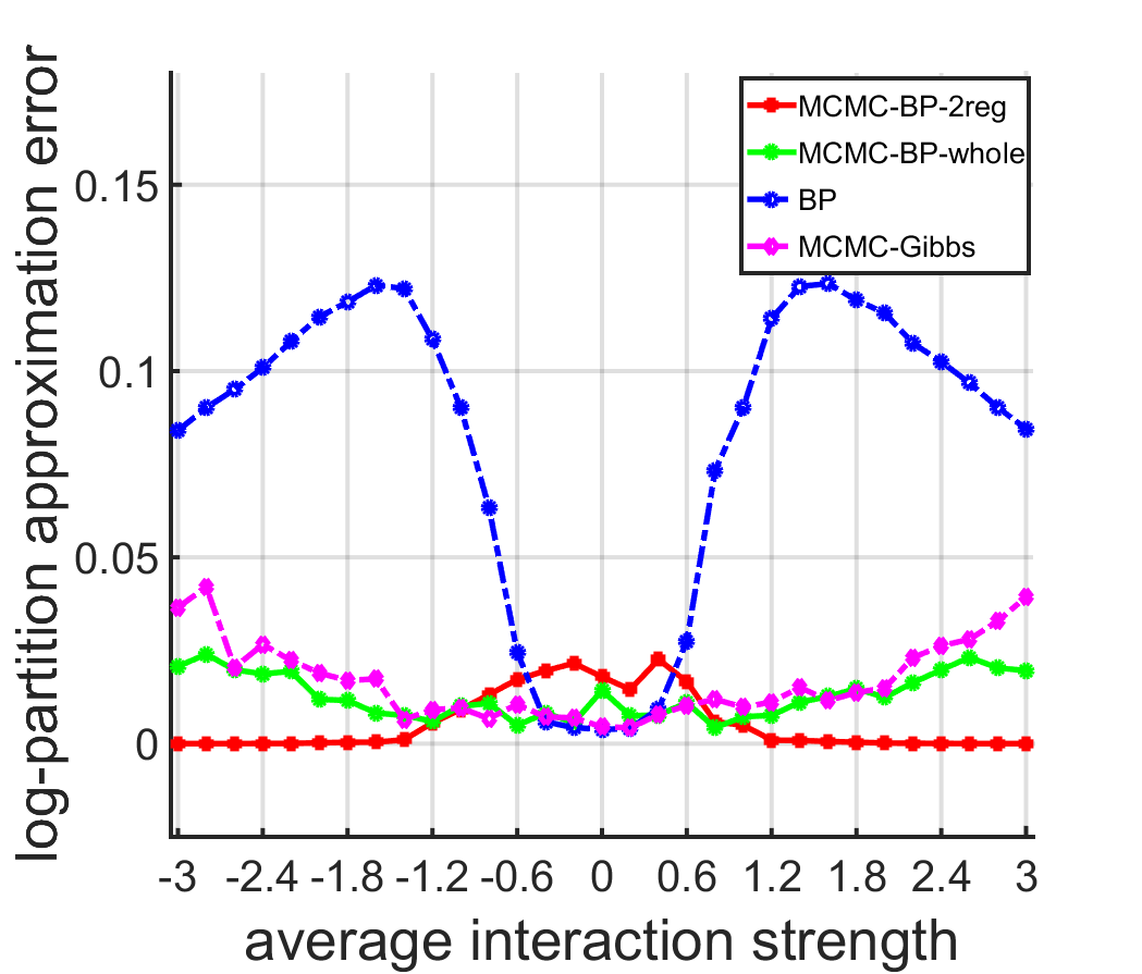
(a)

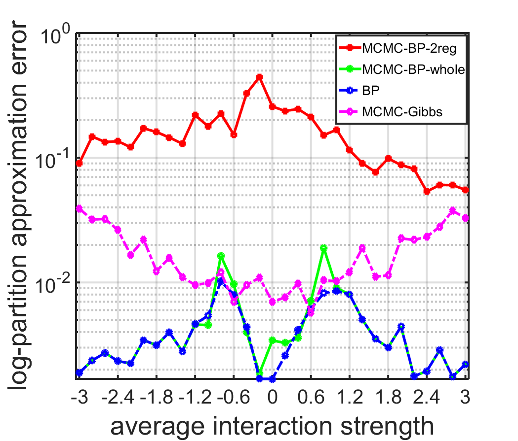
(b)

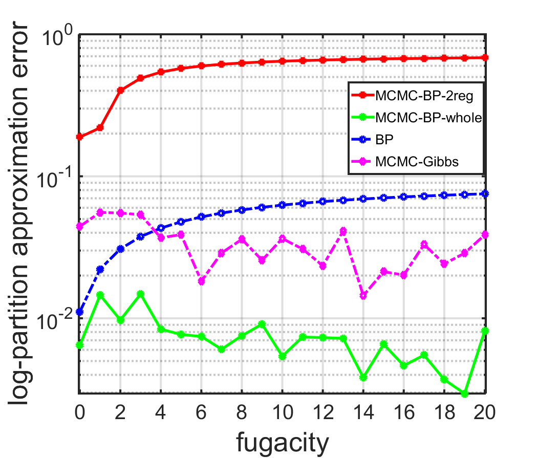
(c)

Figure 1: Plots of the log-partition function approximation error with respect to (average) interaction strength. Each point is averaged over $20$ (random) models.

In this section, we report experimental results for computing partition function of the Ising model and the hard-core model. We compare Algorithm 2 in Section 3 (coined MCMC-BP-2reg) and Algorithm 3 in Section 4.2 (coined MCMC-BP-whole), with the bare Bethe approximation (coined BP) and the popular Gibbs-sampler (coined MCMC-Gibbs). To make the comparison fair, we use the same annealing scheme for all MCMC schemes, thus making their running times comparable. More specifically, we generate each sample after running $T_{1}=1,000$ iterations of an MC and take $s_{1}=100$ samples to compute each estimation (e.g., $H_{i}$) at intermediate steps. For performance measure, we use the log-partition function approximation error defined as $|\log{Z}-\log{Z_{\text{approx}}}|/|\log{Z}|$, where $Z_{\text{approx}}$ is the output of the respective algorithm. We conducted 3 experiments on the $4\times 4$ grid graph. In our first experimental setting, we consider the Ising model with varying interaction strength and no external (magnetic) field. To prepare the model of interest, we start from the Ising model with uniform (ferromagnetic/attractive and anti-ferromagnetic/repulsive) interaction strength and then add ‘glassy’ variability in the interaction strength modeled via i.i.d Gaussian random variables with mean $0$ and variance $0.5^{2}$, i.e. $\mathcal{N}(0,0.5^{2})$. In other words, given average interaction strength $0.3$, each interaction strength in the model is independently chosen as $\mathcal{N}(0.3,0.5^{2})$. The second experiment was conducted by adding $\mathcal{N}(0,0.5^{2})$ corrections to the external fields under the same condition as in the first experiment. In this case we observe that BP often fails to converge, and use the Concave Convex Procedure (CCCP) [23] for finding BP fixed points. Finally, we experiment with the hard-core model on the $4\times 4$ grid graph with varying a positive parameter $\lambda>0$, called ‘fugacity’ [26]. As seen clearly in Figure 1, BP and MCMC-Gibbs are outperformed by MCMC-BP-2reg or MCMC-BP-whole at most tested regimes in the first experiment with no external field, where in this case, the 2-regular loop series (LS) is equal to the full one. Even in the regimes where MCMC-Gibbs outperforms BP, our schemes correct the error of BP and performs at least as good as MCMC-Gibbs. In the experiments, we observe that advantage of our schemes over BP is more pronounced when the error of BP is large. A theoretical reasoning behind this observation is as follows. If the performance of BP is good, i.e. the loop series (LS) is close to $1$, the contribution of empty generalized loop, i.e., $w(\emptyset)$, in LS is significant, and it becomes harder to sample other generalized loops accurately.

5 Conclusion

In this paper, we propose new MCMC schemes for approximate inference in GMs. The main novelty of our approach is in designing BP-aware MCs utilizing the non-trivial BP solutions. In experiments, our BP based MCMC scheme also outperforms other alternatives. We anticipate that this new technique will be of interest to many applications where GMs are used for statistical reasoning.

A Transformation to an equivalent binary pairwise model with maximum degree at most 3

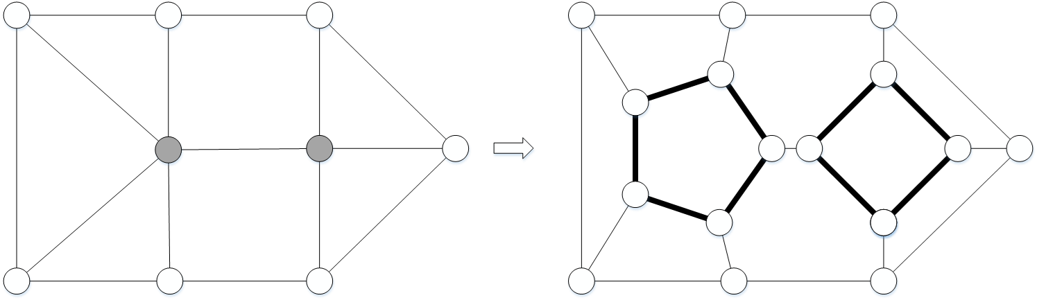
Figure 2: Demonstration of building an equivalent model with maximum degree $\Delta\leq 3$ via ‘expanding’ vertices (in grey). In the new model, one can introduce edge factor $\psi_{u,v}$ between the duplicated vertices $u,v$ (in bold) such that $\psi_{u,v}(x_{u},x_{v})=1$ if $x_{u}=x_{v}$ and $\psi_{u,v}(x_{u},x_{v})=0$ otherwise.

B Proof of Theorem 1

First, note that the MC induced by the worm algorithm converges to the following stationary distribution

$$\pi_{\text{WA}}(F)\propto\Psi(F)\prod_{e\in F}w(e),$$

where

$$\Psi(F)=\begin{cases}n,\qquad&\forall F\in\mathcal{L}_{\text{2-Loop}},\\ 2,\qquad&\forall F\in\mathcal{L}_{\text{2-Odd}}.\end{cases}$$

We first prove its polynomial mixing, i.e. it produces a sample from a distribution with the desired total variation distance from $\pi_{\text{WA}}$ in a polynomial number of iterations.

Lemma 1.

Given any $\delta>0$ and any $F_{0}\in\mathcal{L}_{\text{2-Loop}}\cup\mathcal{L}_{\text{2-Loop}}$, choose

$$T_{\text{mix}}\geq w(F_{0})^{-1}+(m-n+1)\log 2+12\Delta mn^{4}\log\delta^{-1},$$

and let $\pi^{t}_{\text{WA}}(\cdot)$ denote the resulting distribution of after updating $t$ times by the worm algorithm with initial state $F_{0}$. Then, it follows that

$$\frac{1}{2}\sum_{F\in\mathcal{L}_{\text{2-Loop}}\cup\mathcal{L}_{\text{2-Loop}}}\bigg{|}\pi^{T_{\text{mix}}}_{\text{WA}}(F)-\pi_{\text{WA}}(F)\bigg{|}\leq\delta,$$

namely, the mixing time of the MC is bounded above by $T_{\text{mix}}$.

The proof of the above lemma is given in Section B.1. Collevecchio et al. [18] recently proved that the worm algorithm mixes in polynomial time when the weights are uniform, i.e., equal. We extend the result to our case of non-uniform weights. The proof is based on the method of canonical path, which views the state space as a graph and constructs a path between every pair of states having certain amount of flow defined by $\pi_{\text{WA}}$. From Lemma 1 with parameters

$$N\leq 1.2n\log(3\delta^{-1}),\quad T\leq(m-n+1)\log 2+4\Delta mn^{4}\log(3n\delta^{-1}),\quad\mbox{and}\quad F_{0}\leftarrow\emptyset,$$

we obtain that the total variation distance between $\pi_{\text{WA}}$ and the distribution of updated states in line 4 of Algorithm 1 is at most $\frac{\delta}{3n}$. Next, we prove that the probability of acceptance in line $6$ of Algorithm 1 is sufficiently large.

Lemma 2.

The probability of sampling a $2$-regular loop from distribution $\pi_{WA}$ is bounded below by $n^{-1}$, i.e. $\pi_{\text{WA}}(\mathcal{L}_{\text{2-Loop}})\geq\frac{1}{n}.$

The proof of the above lemma is given in Section B.2. The proof relies on the fact that the size of $\mathcal{L}_{\text{2-Loop}}$ is bounded by a polynomial of the size of $\mathcal{L}_{\text{2-Odd}}$.

Now we are ready to complete the proof of Theorem 1. Let $\widehat{\pi}_{\text{2-Loop}}$ denote the distribution of $2$-regular loops from line 6 of Algorithm 1 under parameters as in Theorem 1. We say Algorithm 1 fails if it outputs $F=\emptyset$ from line 9. Choose a set of $2$-regular loops $\widehat{\mathcal{L}}_{\text{2-Loop}}:=\{F\in\mathcal{L}_{\text{2-Loop}}:\widehat{\pi}_{\text{2-Loop}}(F)>\pi_{\text{2-Loop}}(F)\}.$ Then the total variation distance between $\pi_{\text{2-Loop}}$ and $\widehat{\pi}_{\text{2-Loop}}$ can be expressed as:

$$\frac{1}{2}\sum_{F\in\mathcal{L}_{\text{2-Loop}}}|\widehat{\pi}_{\text{2-Loop}}(F)-\pi_{\text{2-Loop}}(F)|=\widehat{\pi}_{\text{2-Loop}}(\widehat{\mathcal{L}}_{\text{2-Loop}})-\pi_{\text{2-Loop}}(\widehat{\mathcal{L}}_{\text{2-Loop}}).$$

By applying Lemma 1 and Lemma 2, we obtain the following under parameters as in Theorem 1:

$$\widehat{\pi}_{\text{2-Loop}}(\widehat{\mathcal{L}}_{\text{2-Loop}})-\pi_{\text{2-Loop}}(\widehat{\mathcal{L}}_{\text{2-Loop}})$$

$$\qquad\stackrel{{\scriptstyle(a)}}{{\geq}}~{}\frac{\widehat{\pi}_{\text{WA}}(\widehat{\mathcal{L}}_{\text{2-Loop}})}{\widehat{\pi}_{\text{WA}}(\mathcal{L}_{\text{2-Loop}})}-(1-\widehat{\pi}_{\text{WA}}(\mathcal{L}_{\text{2-Loop}}))^{N}-\pi_{\text{2-Loop}}(\widehat{\mathcal{L}}_{\text{2-Loop}})$$

$$\qquad\stackrel{{\scriptstyle(b)}}{{\geq}}~{}\frac{\pi_{\text{WA}}(\widehat{\mathcal{L}}_{\text{2-Loop}})+\frac{\delta}{3n}}{\pi_{\text{WA}}(\mathcal{L}_{\text{2-Loop}})-\frac{\delta}{3n}}-(1-\pi_{\text{WA}}(\mathcal{L}_{\text{2-Loop}})-\frac{\delta}{3n})^{N}-\pi_{\text{2-Loop}}(\widehat{\mathcal{L}}_{\text{2-Loop}})$$

$$\qquad\stackrel{{\scriptstyle(c)}}{{\geq}}~{}-\frac{2\delta}{3n\,\pi_{\text{WA}}(\mathcal{L}_{\text{2-Loop}})}-e^{-(\pi_{\text{WA}}(\mathcal{L}_{\text{2-Loop}})+\frac{\delta}{3n})N}$$

$$\qquad\stackrel{{\scriptstyle(d)}}{{\geq}}~{}-\frac{2\delta}{3}-\frac{\delta}{3}=-\delta.$$

In the above, (a) comes from the fact that a sample from line 6 of Algorithm 1 follows the distribution $\frac{\widehat{\pi}_{\text{WA}}(\widehat{\mathcal{L}}_{\text{2-Loop}})}{\widehat{\pi}_{\text{WA}}(\mathcal{L}_{\text{2-Loop}})}$ and the failure probability of Algorithm 1 is $(1-\widehat{\pi}_{\text{WA}}(\mathcal{L}_{\text{2-Loop}}))^{N}$. For (b), we use the variation distance between $\widehat{\pi}_{\text{WA}}$ and $\pi_{\text{WA}}$ due to Lemma 1 and parameters as in Theorem 1, i.e.,

$$|\widehat{\pi}_{\text{WA}}(S)-\pi_{\text{WA}}(S)|\leq\frac{\delta}{3n}\qquad\forall~{}S\subseteq\mathcal{L}_{\text{2-Loop}}\cup\mathcal{L}_{\text{2-Odd}}.$$

For (c), we use $(1-x)\leq e^{-x}$ for any $x\geq 0$ and (d) follows from Lemma 2 and $N\leq n\ln(3\delta^{-1})$. The converse $\widehat{\pi}_{\text{2-Loop}}(\widehat{\mathcal{L}}_{\text{2-Loop}})-\pi_{\text{2-Loop}}(\widehat{\mathcal{L}}_{\text{2-Loop}})\leq\delta$ can be done similarly by considering the complementary set $\mathcal{L}_{\text{2-Loop}}\backslash\widehat{\mathcal{L}}_{\text{2-Loop}}$. This completes the proof of Theorem 1.

B.1 Proof of Lemma 1

First, let $P_{\text{WA}}$ denote the transition matrix of MC induced by the worm algorithm in Section 3.1. Then we are able to define the corresponding transition graph $\mathcal{G}_{\text{WA}}=(\mathcal{L}_{\text{2-Loop}}\cup\mathcal{L}_{\text{2-Odd}},\mathcal{E}_{\text{WA}})$, where each vertex is a state of the MC, and edges are defined on state pairs with nonzero transition probability, i.e.

$$\mathcal{E}_{\text{WA}}=\{(A,A^{\prime}):(A,A^{\prime})\in(\mathcal{L}_{\text{2-Loop}}\cup\mathcal{L}_{\text{2-Odd}})\times(\mathcal{L}_{\text{2-Loop}}\cup\mathcal{L}_{\text{2-Odd}}),P_{\pi_{\text{WA}}}(A,A^{\prime})>0\}.$$

Our proof makes use of the following result proved in [18].

Theorem 4 (Schweinsberg 2002 [18]).

Consider an irreducible and lazy MC, with finite state space $\Omega$, transition matrix $P$ and transition graph $\mathcal{G}_{P}$, which is reversible with respect to the distribution $\pi$. Let $\mathcal{O}\subseteq\Omega$ be nonempty, and for each pair $(I,J)\in\Omega\times\mathcal{O}$, specify a path $\gamma_{I,J}$ in $\mathcal{G}_{P}$ from $I$ to $J$. Let

$$\Gamma=\{\gamma_{I,J}:(I,J)\in\Omega\times\mathcal{O}\}$$

denote the collection of all such paths, and let $L(\Gamma)$ be the length of longest path in $\Gamma$. For any transition $T\in\mathcal{E}_{P}$, let

$$\mathcal{H}_{T}=\{(I,F)\in\Omega\times\mathcal{O}:T\in\gamma_{I,J}\}.$$

Then

$$\tau_{A}(\delta)\leq\left[\log\left(\frac{1}{\pi(A)+\log\left(\frac{1}{\delta}\right)}\right)\right]4L(T)\Phi(\Gamma)$$

where

$$\Phi(\Gamma)=\max_{(A,A^{\prime})\in\mathcal{E}_{P}}\left\{\sum_{I,J\in\mathcal{H}_{(A,A^{\prime})}}\frac{\pi(I)\pi(J)}{\pi(\mathcal{O})\pi(A)P(A,A^{\prime})}\right\}.$$

To this end, we choose $\mathcal{O}=\mathcal{L}_{\text{2-Loop}}$ and we show that there exists a choice of paths $\Gamma=\{\gamma_{I,J}:(I,J)\in(\mathcal{L}_{\text{2-Loop}}\cup\mathcal{L}_{\text{2-Loop}})\times\mathcal{L}_{\text{2-Odd}}\}$ such that

$$\Phi(\Gamma)\leq\Delta n^{4},\qquad L(\Gamma)\leq m.$$

Then we obtain the statement in Lemma 1 immediately.

We begin by specifying $\Gamma$, and then proceed to the bound of $\Phi(\Gamma)$. To this end, we fix an $[n]$-valued vertex labeling of $\mathcal{G}_{\text{WA}}$. The labeling induces a lexicographical total order of the edges, which in turn induces a lexicographical total order on the set of all subgraphs of $\mathcal{G}_{\text{WA}}$. In order for the state $I\in\mathcal{L}_{\text{2-Loop}}\cup\mathcal{L}_{\text{2-Odd}}$ transit to the $J\in\mathcal{L}_{\text{2-Loop}}$, it suffices that it updates, precisely once, those edges in $I\oplus J$. In order to describe such path, we first prove that there exist a injection from $I\oplus J$ to some unique disjoint partition $I\oplus J=\cup^{k}_{i=0}C_{i}$, where $C_{0}$ is either a path or a cycle and $C_{1},\cdots,C_{k}$ are cycles. Observe that since $J\in\mathcal{L}_{\text{2-Loop}}$, applying symmetric difference with $J$ does not change the parity of degrees of the vertices and $I\oplus J\in\mathcal{L}_{\text{2-Loop}}\cup\mathcal{L}_{\text{2-Odd}}$. First consider the case when $I\oplus J\in\mathcal{L}_{\text{2-Odd}}$. Then there exist a path between two odd-degree vertices in $I\oplus J$, since the sum of degrees over all vertices in a component is even. Among such paths, we pick $C_{0}$ as the path with the highest order according to the $[n]$-valued vertex labeling. Now observe that $I\oplus J\backslash C_{0}\in\mathcal{L}_{\text{2-Loop}}$ is Eulerian, which can be decomposed into disjoint set of cycles. We are able to choose a $C_{1},\cdots,C_{k}$ uniquely by recursively excluding a cycle with the highest order, i.e. we pick $C_{1}$ as a cycle with highest order from $I\oplus J\backslash C_{0}$, then pick $C_{2}$ from $I\oplus J\backslash C_{0}\backslash C_{1}$ with the highes order, and so on. For the case when $I\in\mathcal{L}_{\text{2-Loop}}$, $I\oplus J\in\mathcal{L}_{\text{2-Loop}}$ is Eulerian and we can apply similar logic to obtain the unique decomposition into disjoint cycles.

Now we are ready to describe $\gamma_{I,J}$, which updates the edges in $I\oplus J$ from $C_{0}$ to $C_{k}$ in order. If $C_{0}$ is a path, pick an endpoint with higher order of label and update the edges in the paths by it unwinding the edges along the path until other endpoint is met. In the case of cycles, pick a vertex with highest order of label and unwind the edges by a fixed orientation. Note that during the update of cycles, the number of odd-degree vertices are at most 2, so the intermediate states are stil in $\mathcal{L}_{\text{2-Loop}}\cup L_{\text{2-Odd}}$. As a result, we have constructed a path $\gamma_{I,F}$ for each $I\in\mathcal{L}_{\text{2-Loop}}\cup\mathcal{L}_{\text{2-Odd}}$ and $J\in\mathcal{L}_{\text{2-Loop}}$ where each edge correspond to an update on $I\oplus J$ and $|\gamma_{I,F}|=|I\oplus J|\leq m$.

Next, we bound the corresponding $\Phi(\Gamma)$. First let $\mathcal{L}_{\text{4-Odd}}$ denote the set of subgraphs with exactly $4$ odd-degree vertices. We define a mapping $\eta_{T}:\mathcal{H}_{T}\rightarrow\mathcal{L}_{\text{2-Loop}}\cup\mathcal{L}_{\text{2-Odd}}\cup\mathcal{L}_{\text{4-Odd}}$ by the following:

$$\eta_{T}(I,J):=I\oplus F\oplus(A\cup e),$$

where $T=(A,A\oplus e)$. Observe that $\eta_{T}(I,J)$ agrees with $I$ on the components that have already been processed, and with $J$ on the components that have not. We prove that $\eta_{T}$ is an injection by reconstructing $I$ and $J$ from $\eta_{T}(I,J)$ given $T=(A,A\oplus e)$. To this end, observe that $I\oplus F=\eta_{T}(I,F)\oplus(A\cup e)$ is uniquely decided from $\eta_{T}(I,F)$ and $(A\cup e)$. Then given $I\oplus F$, we are able to infer the decomposition $C_{0},C_{1},\cdots,C_{k}$ of $I\oplus J$ by the rules defined previously. Moreover the updated edge $e$ implies the current set $C_{i}$ being updated. Therefore we can infer the processed part of $I\oplus J$. Then we can recover $J$ by beginning in $A$ and unwinding the remaining edges in $I\oplus J$ that was not processed yet. Then we recover $I$ via $I=\eta_{T}(I,J)\oplus(A\cup e)\oplus J$ and therefore $\eta_{T}$ is injective.

Next, we define a metric $w_{\text{WA}}$ such that given an edge set $F$,

$$w_{\text{WA}}(F):=\prod_{e\in F}|w(e)|.$$

We complete the proof by showing that for any $T=(A,A^{\prime})\in\mathcal{E}$, the following inequality holds:

$$\Phi(\Gamma)\stackrel{{\scriptstyle(a)}}{{\leq}}\sum_{I,J\in\mathcal{H}_{T}}\frac{1}{\pi(\mathcal{L}_{\text{2-Loop}})}\frac{\pi(I)\pi(J)}{\pi(A)P(A,A^{\prime})}\stackrel{{\scriptstyle(b)}}{{\leq}}\sum_{I,J\in\mathcal{H}_{T}}\frac{2\Delta}{w_{\text{WA}}(\mathcal{L}_{\text{2-Loop}})}\Psi(I)w_{\text{WA}}(\eta_{T}(I,J))\stackrel{{\scriptstyle(c)}}{{\leq}}\Delta n^{4}.$$

First, (a) holds by definition of $\Phi$. We prove (b) by the following chain of inequality:

$$\frac{1}{\pi(\mathcal{L}_{\text{2-Loop}})}\frac{\pi(I)\pi(J)}{\pi(A)P(A,A^{\prime})} =\frac{1}{nw_{\text{WA}}(\mathcal{L}_{\text{2-Loop}})}\frac{\Psi(I)w_{\text{WA}}(I)nw_{\text{WA}}(J)}{\Psi(A)w_{\text{WA}}(A)P_{\text{WA}}(A,A^{\prime})}$$

$$\stackrel{{\scriptstyle(1)}}{{\leq}}\frac{1}{w_{\text{WA}}(\mathcal{L}_{\text{2-Loop}})}\Psi(I)w_{\text{WA}}(I)w_{\text{WA}}(J)\frac{2\Delta}{w_{\text{WA}}(A\cup e)}$$

$$\stackrel{{\scriptstyle(2)}}{{=}}\frac{2\Delta}{w_{\text{WA}}(\mathcal{L}_{\text{2-Loop}})}\Psi(I)w_{\text{WA}}(\eta_{T}(I,F)).$$

In the above, (1) comes from the definition of the transition probability and (2) comes from the definition of function $w_{\text{WA}}$. Finally, we prove (c). First, we have

$$\Psi(\Gamma) \leq\sum_{(I,J)\in\mathcal{H}_{T}}\frac{2\Delta}{w_{\text{WA}}(\mathcal{L}_{\text{2-Loop}})}\Psi(I)w_{\text{WA}}(\eta_{T}(I,F))$$

$$\leq\sum_{(I,J)\in\mathcal{H}_{T}}\frac{2\Delta}{w_{\text{WA}}(\mathcal{L}_{\text{2-Loop}})}[w_{\text{WA}}(\mathcal{L}_{\text{2-Loop}}\cup\mathcal{L}_{\text{2-Odd}})+2w_{\text{WA}}(\mathcal{L}_{\text{2-Loop}}\cup\mathcal{L}_{\text{2-Odd}}\cup\mathcal{L}_{\text{4-Odd}})]$$

$$=2\Delta\left[(n+2)+(n+2)+\frac{w_{\text{WA}}(\mathcal{L}_{\text{2-Odd}})}{w_{\text{WA}}(\mathcal{L}_{\text{2-Loop}})}+2\frac{w_{\text{WA}}(\mathcal{L}_{\text{4-Odd}})}{w_{\text{WA}}(\mathcal{L}_{\text{2-Loop}})}\right],$$

since $\eta_{T}(I,J)$ is an injection on $\mathcal{L}_{\text{2-Loop}}\cup\mathcal{L}_{\text{2-Odd}}\cup\mathcal{L}_{\text{4-Odd}}$, and the set $\mathcal{L}_{\text{2-Loop}},\mathcal{L}_{\text{2-Odd}},\mathcal{L}_{\text{4-Odd}}$ are disjoint. Now we prove

$$\frac{w_{\text{WA}}(\mathcal{L}_{\text{2-Odd}})}{w_{\text{WA}}(\mathcal{L}_{\text{2-Loop}})}\leq\binom{n}{2}\qquad\frac{w_{\text{WA}}(\mathcal{L}_{\text{4-Odd}})}{w_{\text{WA}}(\mathcal{L}_{\text{2-Loop}})}\leq\binom{n}{4},$$

which completes the proof of Lemma 1 since $(n+2)+(n+2)+\binom{n}{2}+2\binom{n}{4}\leq\frac{n^{4}}{2}.$ To this end, we let $\mathcal{L}_{\text{Odd}}(W)$ denote the set of generalized loops having $W$ as the set of odd degree vertices. Now observe the following inequality:

$$\sum_{F\in\mathcal{L}_{\text{Odd}}(W)}w_{\text{WA}}(F) \stackrel{{\scriptstyle(a)}}{{=}}~{}\frac{1}{2^{n}}\sum_{F\in\mathcal{L}}\prod_{e\in F}|w(e)|\prod_{s\in V\backslash W}(1+(-1)^{d_{F}(v)})\prod_{s\in W}(1+(-1)^{d_{F}(v)+1})$$

$$=\frac{1}{2^{n}}\sum_{\sigma\in\{-1,1\}^{V}}\sum_{F\in\mathcal{L}}\prod_{e\in F}|w(e)|\prod_{s\in V}\sigma_{v}^{d_{F}(v)}\prod_{v\in W}\sigma_{v}$$

$$=~{}\sum_{\sigma\in\{-1,+1\}^{V}}\prod_{e=(u,v)\in E}(1+|w(e)|\sigma_{u}\sigma_{v})\prod_{v\in W}\sigma_{v}$$

$$\stackrel{{\scriptstyle(b)}}{{\geq}}~{}\sum_{\sigma\in\{-1,+1\}^{V}}\prod_{e=(u,v)\in E}(1+|w(e)|\sigma_{u}\sigma_{v})$$

$$\stackrel{{\scriptstyle(c)}}{{=}}~{}\sum_{F\in\mathcal{L}_{\mathcal{L}_{\text{2-Loop}}}}w_{\text{WA}}(F).$$

In the above, (a) comes from the fact that $1+(-1)^{d_{v}(F)}=2$ if $d_{v}(F)$ is even and $0$ otherwise, so only the terms corresponding to $2$-regular loop becomes non-zero. For (b), the inequality comes from the fact that $1+|w(e)|\sigma_{u}\sigma_{v}\geq 0$ and $\sigma_{v}\leq 1$. For (c), the equality is from the fact that $\mathcal{L}_{\text{2-Loop}}=\mathcal{L}_{\text{Odd}}(\emptyset).$ Therefore we have $\sum_{F\in L(\emptyset)}|w(F)|\geq\sum_{F\in L(W)}|w(F)|$, leading to

$$\frac{w_{\text{WA}}(\mathcal{L}_{\text{2-Odd}})}{w_{\text{WA}}(\mathcal{L}_{\text{2-Loop}})} =\frac{\sum_{W\subseteq V,|W|=2}\sum_{F\in\mathcal{L}_{\text{Odd}}(W)}|w_{\text{WA}}(F)|}{w_{\text{WA}}(\mathcal{L}_{\text{2-Loop}})}\leq\binom{n}{2},$$

and the case for $\mathcal{L}_{\text{4-Odd}}$ is done similarly. This completes the proof of Lemma 1.

B.2 Proof of Lemma 2

Given $W\subseteq V$, we let $\mathcal{L}_{\text{Odd}}(W)$ denote the set of generalized loops having $W$ as the set of odd degree vertices. where $\mbox{Odd}(F)$ is the set of odd-degree vertices in $F$. Now observe the following inequality:

$$\sum_{F\in\mathcal{L}_{\text{Odd}}(W)}w_{\text{WA}}(F) \stackrel{{\scriptstyle(a)}}{{=}}~{}\frac{1}{2^{n}}\sum_{F\in\mathcal{L}}\prod_{e\in F}|w(e)|\prod_{s\in V\backslash W}(1+(-1)^{d_{F}(v)})\prod_{s\in W}(1+(-1)^{d_{F}(v)+1})$$

$$=\frac{1}{2^{n}}\sum_{\sigma\in\{-1,1\}^{V}}\sum_{F\in\mathcal{L}}\prod_{e\in F}|w(e)|\prod_{s\in V}\sigma_{v}^{d_{F}(v)}\prod_{v\in W}\sigma_{v}$$

$$=~{}\sum_{\sigma\in\{-1,+1\}^{V}}\prod_{e=(u,v)\in E}(1+|w(e)|\sigma_{u}\sigma_{v})\prod_{v\in W}\sigma_{v}$$

$$\stackrel{{\scriptstyle(b)}}{{\geq}}~{}\sum_{\sigma\in\{-1,+1\}^{V}}\prod_{e=(u,v)\in E}(1+|w(e)|\sigma_{u}\sigma_{v})$$

$$\stackrel{{\scriptstyle(c)}}{{=}}~{}\sum_{F\in\mathcal{L}_{\mathcal{L}_{\text{2-Loop}}}}w_{\text{WA}}(F).$$

In the above, (a) comes from the fact that $1+(-1)^{d_{v}(F)}=2$ if $d_{v}(F)$ is even and $0$ otherwise, so only the terms corresponding to $2$-regular loop becomes non-zero. For (b), the inequality comes from the fact that $1+|w(e)|\sigma_{u}\sigma_{v}\geq 0$ and $\sigma_{v}\leq 1$. For (c), the equality is from the fact that $\mathcal{L}_{\text{2-Loop}}=\mathcal{L}_{\text{Odd}}(\emptyset).$ Therefore we have $\sum_{F\in L(\emptyset)}|w(F)|\geq\sum_{F\in L(W)}|w(F)|$, leading to

$$\frac{\sum_{F\in\mathcal{L}_{\text{2-Loop}}}\pi_{\text{WA}}(F)}{\sum_{F\in\mathcal{L}_{\text{2-Loop}}\cup\mathcal{L}_{\text{2-Odd}}}\pi_{\text{WA}}(F)} =\frac{n\sum_{F\in\mathcal{L}_{\text{2-Loop}}}|w_{\text{WA}}(F)|}{n\sum_{F\in\mathcal{L}_{\text{2-Loop}}}|w_{\text{WA}}(F)|+\sum_{W_{\text{WA}}\subseteq V,|W|=2}\sum_{F\in\mathcal{L}_{\text{Odd}}(W)}|w_{\text{WA}}(F)|}$$

$$\geq\frac{n}{n+2\binom{n}{2}}=\frac{1}{n},$$

which completes the proof of Lemma 2.

C Proof of Theorem 2

First, we quantify how much samples from Algorithm 1 are necessary for estimating some non-negative real valued function $f$ on $\mathcal{L}_{\text{2-Loop}}$. To this, we state the following lemma which is a straightforward application of the known result in [8].

Lemma 3.

Let $f$ be a non-negative real-valued function defined on $\mathcal{L}_{\text{2-Loop}}$ and bounded above by $f_{\max}\geq 0$. Given $0<\xi\leq 1$ and $0<\eta\leq 1/2$, choose

$$s \geq\frac{504\xi^{-2}\lceil\log\eta^{-1}\rceil f_{\max}}{\mathbb{E}_{\pi_{\text{2-Loop}}}[f]}\qquad N\geq 1.2n\log\frac{24f_{\max}}{\xi\mathbb{E}_{\pi_{\text{2-Loop}}}[f]},$$

$$T \geq(m-n+1)\log 2+4\Delta mn^{4}\log\frac{8f_{\max}}{\xi\mathbb{E}_{\pi_{\text{2-Loop}}}[f]},$$

and generate $2$-regular loops $F_{1},F_{2},\cdots F_{s}$ using Algorithm 1 with inputs $N$ and $T$. Then, it follows that

$$P\bigg{[}\frac{|\frac{1}{s}\sum_{i}|w(F_{i})|-\mathbb{E}_{\pi_{\text{2-Loop}}}(f)|}{\mathbb{E}_{\pi_{\text{2-Loop}}}(f)}\leq\xi\bigg{]}\leq 1-\eta.$$

namely, samples of Algorithm 1 estimates $\mathbb{E}_{\pi_{\text{2-Loop}}}(f)$ within approximation ratio $1\pm\xi$ with probability at least $1-\eta$.

First, recall that during each stage of simulated annealing, we approximate the expectation of the function $w(F)^{1/n}$ with respect to the distribution $\pi_{\text{2-Loop}}(\beta)$, i.e.,

$$\mathbb{E}_{\pi_{\text{2-Loop}}(\beta)}\left[|w(F)|^{1/n}\right]=Z^{\dagger}_{\text{2-Loop}}(\beta_{i+1})/Z^{\dagger}_{\text{2-Loop}}(\beta_{i}).$$

Hence, to apply Lemma 3, we bound $\max_{F}{|w(F)|^{1/n}}$ and $\mathbb{E}_{\pi_{\text{2-Loop}}(\beta)}\left[|w(F)|^{1/n}\right]$ as follows:

$$|w(F)|^{1/n}\leq 1\qquad\qquad\mathbb{E}_{\pi_{\text{2-Loop}}(\beta)}\left[|w(F)|^{1/n}\right]\geq~{}w_{\min},$$

where the first inequality is due to $w(e)\leq 1$ for any $e\in E$ and the second one is from $|F|\leq n$ for any $2$-regular loop $F$. Thus, from Lemma 3 with parameters

$$s\geq 18144n^{2}\varepsilon^{-2}w^{-1}_{\min}\lceil\log(6n\nu^{-1})\rceil,\qquad N\geq 1.2n\log(144n\varepsilon^{-1}w_{\min}^{-1}),$$

$$T\geq(m-n+1)\log 2+4\Delta mn^{4}\log(48n\varepsilon^{-1}w_{\min}^{-1}),$$

on each stage, we obtain

$$P\bigg{[}\frac{|H_{i}-Z^{\dagger}_{\text{2-Loop}}(\beta_{i+1})/Z^{\dagger}_{\text{2-Loop}}(\beta_{i})|}{Z^{\dagger}_{\text{2-Loop}}(\beta_{i+1})/Z^{\dagger}_{\text{2-Loop}}(\beta_{i})}\leq\frac{\varepsilon}{6n}\bigg{]}\geq 1-\frac{\nu}{6n}.$$

This implies that the product $\prod_{i}H_{i}$ estimates $\frac{Z^{\dagger}_{\text{2-Loop}}}{2^{m-n+1}}$ within approximation ratio in

$$[((1-\varepsilon/6n)^{n},(1+\varepsilon/6n)^{n}]\subseteq[1-\varepsilon/3,1+\varepsilon/3]$$

with probability at least $(1-\nu/6n)^{n}\geq 1-\nu/3$, i.e.,

$$P\bigg{[}\frac{|2^{m-n+1}\prod_{i}H_{i}-Z^{\dagger}_{\text{2-Loop}}|}{Z^{\dagger}_{\text{2-Loop}}}\leq\frac{\varepsilon}{3}\bigg{]}\geq 1-\frac{\nu}{3}.$$

Next we define a non-negative real-valued random function $g$ on $\mathcal{L_{\text{2-Loop}}}$ as

$$g(F)=\begin{cases}1\qquad\mbox{if $w(F)<0$}\\ 0\qquad\mbox{otherwise}\end{cases},$$

namely, $\mathbb{E}_{\pi_{\text{2-Loop}}}\left[g(F)\right]=P_{\pi_{\text{2-Loop}}}[w(F)<0]$. Since $\max_{F}{g(F)}=1$, one can apply Lemma 3 with parameters

$$s\geq 18144\zeta(1-2\zeta)^{-2}\varepsilon^{-2}\lceil\log(3\nu^{-1})\rceil,\qquad\qquad\qquad N\geq 1.2n\log(144\varepsilon^{-1}(1-2\zeta)^{-1}),$$

$$T\geq(m-n+1)\log 2+4\Delta mn^{4}\log(48\varepsilon^{-1}(1-2\zeta)^{-1})$$

and have

$$P\bigg{[}\frac{|\kappa-P_{\pi_{\text{2-Loop}}}[w(F)<0]|}{P_{\pi_{\text{2-Loop}}}[w(F)<0]}\leq\frac{(1-2P_{\pi_{\text{2-Loop}}}[w(F)<0])\varepsilon}{6P_{\pi_{\text{2-Loop}}}[w(F)<0]}\bigg{]}\geq 1-\frac{\nu}{3},$$

since $\zeta=P_{\pi_{\text{2-Loop}}}[w(F)<0]$. Furthermore, after some algebraic calculations, one can obtain

$$P\bigg{[}\frac{|(1-2\kappa)-(1-2P_{\pi_{\text{2-Loop}}}[w(F)<0])|}{1-2P_{\pi_{\text{2-Loop}}}[w(F)<0]}\leq\frac{\varepsilon}{3}\bigg{]}\geq 1-\frac{\nu}{3}.$$

The rest of the proof is straightforward since we estimate $Z_{\text{2-Loop}}=(1-2P_{\pi_{\text{2-Loop}}}[w(F)<0])Z^{\dagger}_{\text{2-Loop}}$ by $(1-2\kappa)2^{m-n+1}\prod_{i}H_{i}$, the approximation ratio is in $[(1-\varepsilon/3)^{2},(1+\varepsilon/3)^{2}]\subseteq[1-\varepsilon,1+\varepsilon]$ with probability at least $(1-\nu/3)^{2}\geq 1-\nu$.

D Proof of Theorem 3

Given $F\in\mathcal{L}$, we let the odd-degree vertices in $F$ (i.e., $d_{F}(\cdot)$ is odd) by $v_{1},v_{2},\cdots v_{2\ell}$ for some integer $\ell\geq 0$. Since we assume $G$ is connected, there exist a set of paths $P_{1},P_{2},\cdots P_{\ell}$ such that $P_{i}$ is a path from $v_{2i-1}$ to $v_{2i}$. Note that given any set of edges $D\subseteq E$, $D\oplus P_{i}$ changes the parities of $d_{D}(v_{2i-1}),d_{D}(v_{2i})$, while others remain same. Therefore, all degrees in $F\oplus P_{1}\oplus\cdots\oplus P_{\ell}$ become even. Then, due to the definition of cycle basis, there exist some $C_{1},C_{2},\cdots C_{k}\in\mathcal{C}$ such that

$$C_{1}\oplus C_{2}\cdots\oplus C_{k}=F\oplus P_{1}\oplus\cdots\oplus P_{\ell},$$

namely,

$$F=C_{1}\oplus C_{2}\cdots\oplus C_{k}\oplus P_{1}\oplus\cdots\oplus P_{\ell}.$$

This completes the proof of Theorem 3.

References

• [1] J. Pearl, β€œProbabilistic reasoning in intelligent systems: networks of plausible inference,” Morgan Kaufmann, 2014.
• [2] R. G. Gallager, β€œLow-density parity-check codes,” Information Theory, IRE Transactions 8(1): 21-28, 1962.
• [3] R. F. Kschischang, and J. F. Brendan, β€œIterative decoding of compound codes by probability propagation in graphical models,” Selected Areas in Communications, IEEE Journal 16(2): 219-230, 1998.
• [4] M. I. Jordan, ed. β€œLearning in graphical models,” Springer Science & Business Media 89, 1998.
• [5] R.J. Baxter, β€œExactly solved models in statistical mechanics,” Courier Corporation, 2007.
• [6] W.T. Freeman, C.P. Egon, and T.C. Owen, β€œLearning low-level vision.” International journal of computer vision 40(1): 25-47, 2000.
• [7] V. Chandrasekaran, S. Nathan, and H. Prahladh, β€œComplexity of Inference in Graphical Models,” Association for Uncertainty and Artificial Intelligence, 2008
• [8] M. Jerrum, and A. Sinclair, β€œPolynomial-time approximation algorithms for the Ising model,” SIAM Journal on computing 22(5): 1087-1116, 1993.
• [9] C. Andrieu, N. Freitas, A. Doucet, and M. I. Jordan, β€œAn introduction to MCMC for machine learning,” Machine learning 50(1-2), 5-43, 2003.
• [10] J. Pearl, β€œReverend Bayes on inference engines: A distributed hierarchical approach,” Association for the Advancement of Artificial Intelligence, 1982.
• [11] M. Chertkov, and V. Y. Chernyak, β€œLoop series for discrete statistical models on graphs,” Journal of Statistical Mechanics: Theory and Experiment 2006(6): P06009, 2006.
• [12] M. Chertkov, V. Y. Chernyak, and R. Teodorescu, β€œBelief propagation and loop series on planar graphs,” Journal of Statistical Mechanics: Theory and Experiment 2008(5): P05003, 2008.
• [13] V. Gomez, J. K. Hilbert, and M. Chertkov, β€œApproximate inference on planar graphs using Loop Calculus and Belief Propagation,” The Journal of Machine Learning Research, 11: 1273-1296, 2010.
• [14] P. W. Kasteleyn, β€œThe statistics of dimers on a lattice,” Classic Papers in Combinatorics. BirkhΓ€user Boston, 281-298, 2009.
• [15] N. Prokof’ev, and B. Svistunov, β€œWorm algorithms for classical statistical models,” Physical review letters 87(16): 160601, 2001.
• [16] J.D. Horton, β€œA polynomial-time algorithm to find the shortest cycle basis of a graph.” SIAM Journal on Computing 16(2): 358-366, 1987. APA
• [17] H. A. Kramers, and G. H. Wannier, β€œStatistics of the two-dimensional ferromagnet. Part II,” Physical Review 60(3): 263, 1941.
• [18] A. Collevecchio, T. M. Garoni, T.Hyndman, and D. Tokarev, β€œThe worm process for the Ising model is rapidly mixing,” arXiv preprint arXiv:1509.03201, 2015.
• [19] S. Kirkpatrick, β€œOptimization by simulated annealing: Quantitative studies.” Journal of statistical physics 34(5-6): 975-986, 1984.
• [20] R. Nicholas, β€œThe Bethe partition function of log-supermodular graphical models,” Advances in Neural Information Processing Systems. 2012.
• [21] J. Bang, J., and G. Z. Gutin. β€œDigraphs: theory, algorithms and applications.” Springer Science & Business Media, 2008.
• [22] Y. W. Teh and M. Welling, β€œBelief optimization for binary networks: a stable alternative to loopy belief propagation,” Proceedings of the Eighteenth conference on Uncertainty in artificial intelligence, 493-500, 2001.
• [23] A. L. Yuille, β€œCCCP algorithms to minimize the Bethe and Kikuchi free energies: Convergent alternatives to belief propagation,” Neural Computation, 14(7): 1691-1722, 2002.
• [24] J. Shin, β€œThe complexity of approximating a Bethe equilibrium,” Information Theory, IEEE Transactions on, 60(7): 3959-3969, 2014.
• [25] https://www.quora.com/Statistical-Mechanics-What-is-the-fermion-sign-problem
• [26] Dyer, M., Frieze, A., and Jerrum, M. β€œOn counting independent sets in sparse graphs,” SIAM Journal on Computing 31(5): 1527-1541, 2002.
• [27] J. Schweinsberg, β€œAn $O(n^{2})$ bound for the relaxation time of a Markov chain on cladograms.” Random Structures & Algorithms 20(1): 59-70, 2002.