Density estimation using Real NVP

Abstract

Unsupervised learning of probabilistic models is a central yet challenging problem in machine learning. Specifically, designing models with tractable learning, sampling, inference and evaluation is crucial in solving this task. We extend the space of such models using real-valued non-volume preserving (real NVP) transformations, a set of powerful, stably invertible, and learnable transformations, resulting in an unsupervised learning algorithm with exact log-likelihood computation, exact and efficient sampling, exact and efficient inference of latent variables, and an interpretable latent space. We demonstrate its ability to model natural images on four datasets through sampling, log-likelihood evaluation, and latent variable manipulations.

1 Introduction

The domain of representation learning has undergone tremendous advances due to improved supervised learning techniques. However, unsupervised learning has the potential to leverage large pools of unlabeled data, and extend these advances to modalities that are otherwise impractical or impossible.

One principled approach to unsupervised learning is generative probabilistic modeling. Not only do generative probabilistic models have the ability to create novel content, they also have a wide range of reconstruction related applications including inpainting [61, 46, 59], denoising [3], colorization [71], and super-resolution [9].

As data of interest are generally high-dimensional and highly structured, the challenge in this domain is building models that are powerful enough to capture its complexity yet still trainable. We address this challenge by introducing real-valued non-volume preserving (real NVP) transformations, a tractable yet expressive approach to modeling high-dimensional data.

This model can perform efficient and exact inference, sampling and log-density estimation of data points. Moreover, the architecture presented in this paper enables exact and efficient reconstruction of input images from the hierarchical features extracted by this model.

2 Related work

	Data space ${\mathcal{X}}$		Latent space ${\mathcal{Z}}$
Inference $\begin{aligned} \qquad x&\sim\hat{p}_{X}&\\ \qquad z&=f\left(x\right)\end{aligned}$		$\begin{aligned} \Rightarrow\end{aligned}$
Generation $\begin{aligned} \qquad z&\sim p_{Z}&\\ \qquad x&=f^{-1}\left(z\right)\end{aligned}$		$\begin{aligned} \Leftarrow\end{aligned}$

Figure 1: Real NVP learns an invertible, stable, mapping between a data distribution $\hat{p}_{X}$ and a latent distribution $p_{Z}$ (typically a Gaussian). Here we show a mapping that has been learned on a toy 2-d dataset. The function $f\left(x\right)$ maps samples $x$ from the data distribution in the upper left into approximate samples $z$ from the latent distribution, in the upper right. This corresponds to exact inference of the latent state given the data. The inverse function, $f^{-1}\left(z\right)$, maps samples $z$ from the latent distribution in the lower right into approximate samples $x$ from the data distribution in the lower left. This corresponds to exact generation of samples from the model. The transformation of grid lines in ${\mathcal{X}}$ and ${\mathcal{Z}}$ space is additionally illustrated for both $f\left(x\right)$ and $f^{-1}\left(z\right)$.

Substantial work on probabilistic generative models has focused on training models using maximum likelihood. One class of maximum likelihood models are those described by probabilistic undirected graphs, such as Restricted Boltzmann Machines [58] and Deep Boltzmann Machines [53]. These models are trained by taking advantage of the conditional independence property of their bipartite structure to allow efficient exact or approximate posterior inference on latent variables. However, because of the intractability of the associated marginal distribution over latent variables, their training, evaluation, and sampling procedures necessitate the use of approximations like Mean Field inference and Markov Chain Monte Carlo, whose convergence time for such complex models remains undetermined, often resulting in generation of highly correlated samples. Furthermore, these approximations can often hinder their performance [7].

Directed graphical models are instead defined in terms of an ancestral sampling procedure, which is appealing both for its conceptual and computational simplicity. They lack, however, the conditional independence structure of undirected models, making exact and approximate posterior inference on latent variables cumbersome [56]. Recent advances in stochastic variational inference [27] and amortized inference [13, 43, 35, 49], allowed efficient approximate inference and learning of deep directed graphical models by maximizing a variational lower bound on the log-likelihood [45]. In particular, the variational autoencoder algorithm [35, 49] simultaneously learns a generative network, that maps gaussian latent variables $z$ to samples $x$, and a matched approximate inference network that maps samples $x$ to a semantically meaningful latent representation $z$, by exploiting the reparametrization trick [68]. Its success in leveraging recent advances in backpropagation [51, 39] in deep neural networks resulted in its adoption for several applications ranging from speech synthesis [12] to language modeling [8]. Still, the approximation in the inference process limits its ability to learn high dimensional deep representations, motivating recent work in improving approximate inference [42, 48, 55, 63, 10, 59, 34].

Such approximations can be avoided altogether by abstaining from using latent variables. Auto-regressive models [18, 6, 37, 20] can implement this strategy while typically retaining a great deal of flexibility. This class of algorithms tractably models the joint distribution by decomposing it into a product of conditionals using the probability chain rule according to a fixed ordering over dimensions, simplifying log-likelihood evaluation and sampling. Recent work in this line of research has taken advantage of recent advances in recurrent networks [51], in particular long-short term memory [26], and residual networks [25, 24] in order to learn state-of-the-art generative image models [61, 46] and language models [32]. The ordering of the dimensions, although often arbitrary, can be critical to the training of the model [66]. The sequential nature of this model limits its computational efficiency. For example, its sampling procedure is sequential and non-parallelizable, which can become cumbersome in applications like speech and music synthesis, or real-time rendering.. Additionally, there is no natural latent representation associated with autoregressive models, and they have not yet been shown to be useful for semi-supervised learning.

Generative Adversarial Networks (GANs) [21] on the other hand can train any differentiable generative network by avoiding the maximum likelihood principle altogether. Instead, the generative network is associated with a discriminator network whose task is to distinguish between samples and real data. Rather than using an intractable log-likelihood, this discriminator network provides the training signal in an adversarial fashion. Successfully trained GAN models [21, 15, 47] can consistently generate sharp and realistically looking samples [38]. However, metrics that measure the diversity in the generated samples are currently intractable [62, 22, 30]. Additionally, instability in their training process [47] requires careful hyperparameter tuning to avoid diverging behavior.

Training such a generative network $g$ that maps latent variable $z\sim p_{Z}$ to a sample $x\sim p_{X}$ does not in theory require a discriminator network as in GANs, or approximate inference as in variational autoencoders. Indeed, if $g$ is bijective, it can be trained through maximum likelihood using the change of variable formula:

$$p_{X}(x)=p_{Z}(z)\left|\det\left(\frac{\partial g(z)}{\partial z^{T}}\right)\right|^{-1}.$$ (1)

This formula has been discussed in several papers including the maximum likelihood formulation of independent components analysis (ICA) [4, 28], gaussianization [14, 11] and deep density models [5, 50, 17, 3]. As the existence proof of nonlinear ICA solutions [29] suggests, auto-regressive models can be seen as tractable instance of maximum likelihood nonlinear ICA, where the residual corresponds to the independent components. However, naive application of the change of variable formula produces models which are computationally expensive and poorly conditioned, and so large scale models of this type have not entered general use.

3 Model definition

In this paper, we will tackle the problem of learning highly nonlinear models in high-dimensional continuous spaces through maximum likelihood. In order to optimize the log-likelihood, we introduce a more flexible class of architectures that enables the computation of log-likelihood on continuous data using the change of variable formula. Building on our previous work in [17], we define a powerful class of bijective functions which enable exact and tractable density evaluation and exact and tractable inference. Moreover, the resulting cost function does not to rely on a fixed form reconstruction cost such as square error [38, 47], and generates sharper samples as a result. Also, this flexibility helps us leverage recent advances in batch normalization [31] and residual networks [24, 25] to define a very deep multi-scale architecture with multiple levels of abstraction.

3.1 Change of variable formula

Given an observed data variable $x\in X$, a simple prior probability distribution $p_{Z}$ on a latent variable $z\in Z$, and a bijection $f:X\rightarrow Z$ (with $g=f^{-1}$), the change of variable formula defines a model distribution on $X$ by

$$p_{X}(x) =p_{Z}\big{(}f(x)\big{)}\left|\det\left(\cfrac{\partial f(x)}{\partial x^{T}}\right)\right|$$ (2)

$$\log\left(p_{X}(x)\right) =\log\Big{(}p_{Z}\big{(}f(x)\big{)}\Big{)}+\log\left(\left|\det\left(\frac{\partial f(x)}{\partial x^{T}}\right)\right|\right),$$ (3)

where $\frac{\partial f(x)}{\partial x^{T}}$ is the Jacobian of $f$ at $x$.

Exact samples from the resulting distribution can be generated by using the inverse transform sampling rule [16]. A sample $z\sim p_{Z}$ is drawn in the latent space, and its inverse image $x=f^{-1}(z)=g(z)$ generates a sample in the original space. Computing the density on a point $x$ is accomplished by computing the density of its image $f(x)$ and multiplying by the associated Jacobian determinant $\det\left(\frac{\partial f(x)}{\partial x^{T}}\right)$. See also Figure 1. Exact and efficient inference enables the accurate and fast evaluation of the model.

3.2 Coupling layers

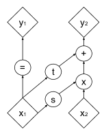
(a) Forward propagation

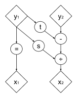
(b) Inverse propagation

Figure 2: Computational graphs for forward and inverse propagation. A coupling layer applies a simple invertible transformation consisting of scaling followed by addition of a constant offset to one part $\mathbf{x}_{2}$ of the input vector conditioned on the remaining part of the input vector $\mathbf{x}_{1}$. Because of its simple nature, this transformation is both easily invertible and possesses a tractable determinant. However, the conditional nature of this transformation, captured by the functions $s$ and $t$, significantly increase the flexibility of this otherwise weak function. The forward and inverse propagation operations have identical computational cost.

Computing the Jacobian of functions with high-dimensional domain and codomain and computing the determinants of large matrices are in general computationally very expensive. This combined with the restriction to bijective functions makes Equation 2 appear impractical for modeling arbitrary distributions.

As shown however in [17], by careful design of the function $f$, a bijective model can be learned which is both tractable and extremely flexible. As computing the Jacobian determinant of the transformation is crucial to effectively train using this principle, this work exploits the simple observation that the determinant of a triangular matrix can be efficiently computed as the product of its diagonal terms.

We will build a flexible and tractable bijective function by stacking a sequence of simple bijections. In each simple bijection, part of the input vector is updated using a function which is simple to invert, but which depends on the remainder of the input vector in a complex way. We refer to each of these simple bijections as an affine coupling layer. Given a $D$ dimensional input $x$ and $d<D$, the output $y$ of an affine coupling layer follows the equations

$$y_{1:d} =x_{1:d}$$ (4)

$$y_{d+1:D} =x_{d+1:D}\odot\exp\big{(}s(x_{1:d})\big{)}+t(x_{1:d}),$$ (5)

where $s$ and $t$ stand for scale and translation, and are functions from $R^{d}\mapsto R^{D-d}$, and $\odot$ is the Hadamard product or element-wise product (see Figure 2(a)).

3.3 Properties

The Jacobian of this transformation is

$$\frac{\partial y}{\partial x^{T}}=\left[\begin{array}[]{cc}{\mathbb{I}}_{d}&0\\ \frac{\partial y_{d+1:D}}{\partial x_{1:d}^{T}}&\operatorname{diag}\big{(}\exp\left[s\left(x_{1:d}\right)\right]\big{)}\end{array}\right],$$ (8)

where $\operatorname{diag}\big{(}\exp\left[s\left(x_{1:d}\right)\right]\big{)}$ is the diagonal matrix whose diagonal elements correspond to the vector $\exp\left[s\left(x_{1:d}\right)\right]$. Given the observation that this Jacobian is triangular, we can efficiently compute its determinant as $\exp\left[\sum_{j}{s\left(x_{1:d}\right)_{j}}\right]$. Since computing the Jacobian determinant of the coupling layer operation does not involve computing the Jacobian of $s$ or $t$, those functions can be arbitrarily complex. We will make them deep convolutional neural networks. Note that the hidden layers of $s$ and $t$ can have more features than their input and output layers.

Another interesting property of these coupling layers in the context of defining probabilistic models is their invertibility. Indeed, computing the inverse is no more complex than the forward propagation (see Figure 2(b)),

$$\begin{cases}y_{1:d}&=x_{1:d}\\ y_{d+1:D}&=x_{d+1:D}\odot\exp\big{(}s(x_{1:d})\big{)}+t(x_{1:d})\end{cases}$$ (9)

$$\Leftrightarrow\begin{cases}x_{1:d}&=y_{1:d}\\ x_{d+1:D}&=\big{(}y_{d+1:D}-t(y_{1:d})\big{)}\odot\exp\big{(}-s(y_{1:d})\big{)},\end{cases}$$ (10)

meaning that sampling is as efficient as inference for this model. Note again that computing the inverse of the coupling layer does not require computing the inverse of $s$ or $t$, so these functions can be arbitrarily complex and difficult to invert.

3.4 Masked convolution

Partitioning can be implemented using a binary mask $b$, and using the functional form for $y$,

$$y=b\odot x+(1-b)\odot\Big{(}x\odot\exp\big{(}s(b\odot x)\big{)}+t(b\odot x)\Big{)}.$$ (11)

We use two partitionings that exploit the local correlation structure of images: spatial checkerboard patterns, and channel-wise masking (see Figure 3). The spatial checkerboard pattern mask has value $1$ where the sum of spatial coordinates is odd, and $0$ otherwise. The channel-wise mask $b$ is $1$ for the first half of the channel dimensions and $0$ for the second half. For the models presented here, both $s(\cdot)$ and $t(\cdot)$ are rectified convolutional networks.

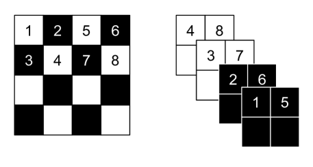
Figure 3: Masking schemes for affine coupling layers. On the left, a spatial checkerboard pattern mask. On the right, a channel-wise masking. The squeezing operation reduces the $4\times 4\times 1$ tensor (on the left) into a $2\times 2\times 4$ tensor (on the right). Before the squeezing operation, a checkerboard pattern is used for coupling layers while a channel-wise masking pattern is used afterward.

3.5 Combining coupling layers

Although coupling layers can be powerful, their forward transformation leaves some components unchanged. This difficulty can be overcome by composing coupling layers in an alternating pattern, such that the components that are left unchanged in one coupling layer are updated in the next (see Figure 4(a)).

The Jacobian determinant of the resulting function remains tractable, relying on the fact that

$$\cfrac{\partial(f_{b}\circ f_{a})}{\partial x_{a}^{T}}(x_{a}) =\cfrac{\partial f_{a}}{\partial x_{a}^{T}}(x_{a})\cdot\cfrac{\partial f_{b}}{\partial x_{b}^{T}}\big{(}x_{b}=f_{a}(x_{a})\big{)}$$ (12)

$$\det(A\cdot B) =\det(A)\det(B).$$ (13)

Similarly, its inverse can be computed easily as

$$(f_{b}\circ f_{a})^{-1}=f_{a}^{-1}\circ f_{b}^{-1}.$$ (14)

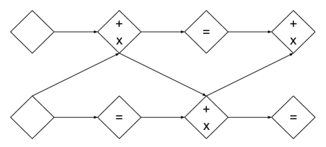
(a) In this alternating pattern, units which remain identical in one transformation are modified in the next.

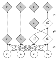
(b) Factoring out variables. At each step, half the variables are directly modeled as Gaussians, while the other half undergo further transformation.

Figure 4: Composition schemes for affine coupling layers.

3.6 Multi-scale architecture

We implement a multi-scale architecture using a squeezing operation: for each channel, it divides the image into subsquares of shape $2\times 2\times c$, then reshapes them into subsquares of shape $1\times 1\times 4c$. The squeezing operation transforms an $s\times s\times c$ tensor into an $\frac{s}{2}\times\frac{s}{2}\times 4c$ tensor (see Figure 3), effectively trading spatial size for number of channels.

At each scale, we combine several operations into a sequence: we first apply three coupling layers with alternating checkerboard masks, then perform a squeezing operation, and finally apply three more coupling layers with alternating channel-wise masking. The channel-wise masking is chosen so that the resulting partitioning is not redundant with the previous checkerboard masking (see Figure 3). For the final scale, we only apply four coupling layers with alternating checkerboard masks.

Propagating a $D$ dimensional vector through all the coupling layers would be cumbersome, in terms of computational and memory cost, and in terms of the number of parameters that would need to be trained. For this reason we follow the design choice of [57] and factor out half of the dimensions at regular intervals (see Equation 16). We can define this operation recursively (see Figure 4(b)),

$$h^{(0)} =x$$ (15)

$$(z^{(i+1)},h^{(i+1)}) =f^{(i+1)}(h^{(i)})$$ (16)

$$z^{(L)} =f^{(L)}(h^{(L-1)})$$ (17)

$$z =(z^{(1)},\dots,z^{(L)}).$$ (18)

In our experiments, we use this operation for $i<L$. The sequence of coupling-squeezing-coupling operations described above is performed per layer when computing $f^{(i)}$ (Equation 16). At each layer, as the spatial resolution is reduced, the number of hidden layer features in $s$ and $t$ is doubled. All variables which have been factored out at different scales are concatenated to obtain the final transformed output (Equation 18).

As a consequence, the model must Gaussianize units which are factored out at a finer scale (in an earlier layer) before those which are factored out at a coarser scale (in a later layer). This results in the definition of intermediary levels of representation [53, 49] corresponding to more local, fine-grained features as shown in Appendix D.

Moreover, Gaussianizing and factoring out units in earlier layers has the practical benefit of distributing the loss function throughout the network, following the philosophy similar to guiding intermediate layers using intermediate classifiers [40]. It also reduces significantly the amount of computation and memory used by the model, allowing us to train larger models.

3.7 Batch normalization

To further improve the propagation of training signal, we use deep residual networks [24, 25] with batch normalization [31] and weight normalization [2, 54] in $s$ and $t$. As described in Appendix E we introduce and use a novel variant of batch normalization which is based on a running average over recent minibatches, and is thus more robust when training with very small minibatches.

We also use apply batch normalization to the whole coupling layer output. The effects of batch normalization are easily included in the Jacobian computation, since it acts as a linear rescaling on each dimension. That is, given the estimated batch statistics $\tilde{\mu}$ and $\tilde{\sigma}^{2}$, the rescaling function

$$x\mapsto\frac{x-\tilde{\mu}}{\sqrt{\tilde{\sigma}^{2}+\epsilon}}$$ (19)

has a Jacobian determinant

$$\left(\prod_{i}{(\tilde{\sigma}_{i}^{2}+\epsilon)}\right)^{-\frac{1}{2}}.$$ (20)

This form of batch normalization can be seen as similar to reward normalization in deep reinforcement learning [44, 65].

We found that the use of this technique not only allowed training with a deeper stack of coupling layers, but also alleviated the instability problem that practitioners often encounter when training conditional distributions with a scale parameter through a gradient-based approach.

4 Experiments

4.1 Procedure

The algorithm described in Equation 2 shows how to learn distributions on unbounded space. In general, the data of interest have bounded magnitude. For examples, the pixel values of an image typically lie in $[0,256]^{D}$ after application of the recommended jittering procedure [64, 62]. In order to reduce the impact of boundary effects, we instead model the density of $\mbox{logit}(\alpha+(1-\alpha)\odot\frac{x}{256})$, where $\alpha$ is picked here as $.05$. We take into account this transformation when computing log-likelihood and bits per dimension. We also augment the CIFAR-10, CelebA and LSUN datasets during training to also include horizontal flips of the training examples.

We train our model on four natural image datasets: CIFAR-10 [36], Imagenet [52], Large-scale Scene Understanding (LSUN) [70], CelebFaces Attributes (CelebA) [41]. More specifically, we train on the downsampled to $32\times 32$ and $64\times 64$ versions of Imagenet [46]. For the LSUN dataset, we train on the bedroom, tower and church outdoor categories. The procedure for LSUN is the same as in [47]: we downsample the image so that the smallest side is $96$ pixels and take random crops of $64\times 64$. For CelebA, we use the same procedure as in [38]: we take an approximately central crop of $148\times 148$ then resize it to $64\times 64$.

We use the multi-scale architecture described in Section 3.6 and use deep convolutional residual networks in the coupling layers with rectifier nonlinearity and skip-connections as suggested by [46]. To compute the scaling functions $s$, we use a hyperbolic tangent function multiplied by a learned scale, whereas the translation function $t$ has an affine output. Our multi-scale architecture is repeated recursively until the input of the last recursion is a $4\times 4\times c$ tensor. For datasets of images of size $32\times 32$, we use $4$ residual blocks with $32$ hidden feature maps for the first coupling layers with checkerboard masking. Only $2$ residual blocks are used for images of size $64\times 64$. We use a batch size of $64$. For CIFAR-10, we use $8$ residual blocks, $64$ feature maps, and downscale only once. We optimize with ADAM [33] with default hyperparameters and use an $L_{2}$ regularization on the weight scale parameters with coefficient $5\cdot 10^{-5}$.

We set the prior $p_{Z}$ to be an isotropic unit norm Gaussian. However, any distribution could be used for $p_{Z}$, including distributions that are also learned during training, such as from an auto-regressive model, or (with slight modifications to the training objective) a variational autoencoder.

4.2 Results

Dataset	PixelRNN [46]	Real NVP	Conv DRAW [22]	IAF-VAE [34]
CIFAR-10	3.00	3.49	< 3.59	< 3.28
Imagenet ($32\times 32$)	3.86 (3.83)	4.28 (4.26)	< 4.40 (4.35)
Imagenet ($64\times 64$)	3.63 (3.57)	3.98 (3.75)	< 4.10 (4.04)
LSUN (bedroom)		2.72 (2.70)
LSUN (tower)		2.81 (2.78)
LSUN (church outdoor)		3.08 (2.94)
CelebA		3.02 (2.97)

Table 1: Bits/dim results for CIFAR-10, Imagenet, LSUN datasets and CelebA. Test results for CIFAR-10 and validation results for Imagenet, LSUN and CelebA (with training results in parenthesis for reference).

We show in Table 1 that the number of bits per dimension, while not improving over the Pixel RNN [46] baseline, is competitive with other generative methods. As we notice that our performance increases with the number of parameters, larger models are likely to further improve performance. For CelebA and LSUN, the bits per dimension for the validation set was decreasing throughout training, so little overfitting is expected.

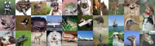
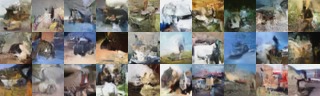
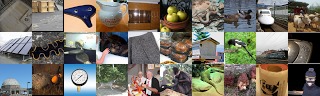
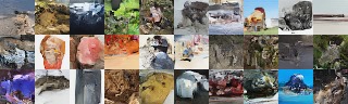
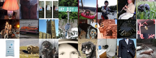
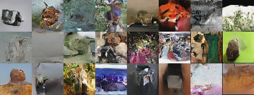
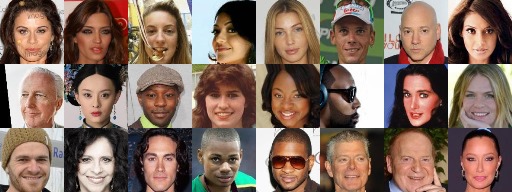
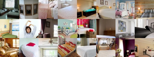
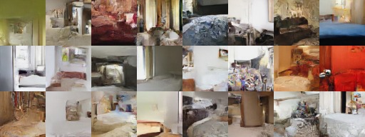
Figure 5: On the left column, examples from the dataset. On the right column, samples from the model trained on the dataset. The datasets shown in this figure are in order: CIFAR-10, Imagenet ($32\times 32$), Imagenet ($64\times 64$), CelebA, LSUN (bedroom).

We show in Figure 5 samples generated from the model with training examples from the dataset for comparison. As mentioned in [62, 22], maximum likelihood is a principle that values diversity over sample quality in a limited capacity setting. As a result, our model outputs sometimes highly improbable samples as we can notice especially on CelebA. As opposed to variational autoencoders, the samples generated from our model look not only globally coherent but also sharp. Our hypothesis is that as opposed to these models, real NVP does not rely on fixed form reconstruction cost like an $L_{2}$ norm which tends to reward capturing low frequency components more heavily than high frequency components. Unlike autoregressive models, sampling from our model is done very efficiently as it is parallelized over input dimensions. On Imagenet and LSUN, our model seems to have captured well the notion of background/foreground and lighting interactions such as luminosity and consistent light source direction for reflectance and shadows.

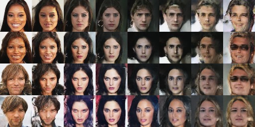
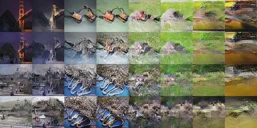
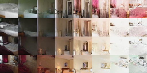
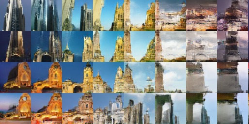
Figure 6: Manifold generated from four examples in the dataset. Clockwise from top left: CelebA, Imagenet ($64\times 64$), LSUN (tower), LSUN (bedroom).

We also illustrate the smooth semantically consistent meaning of our latent variables. In the latent space, we define a manifold based on four validation examples $z_{(1)}$, $z_{(2)}$, $z_{(3)}$, $z_{(4)}$, and parametrized by two parameters $\phi$ and $\phi^{\prime}$ by,

$$z=\cos(\phi)\left(\cos(\phi^{\prime})z_{(1)}+\sin(\phi^{\prime})z_{(2)}\right)+\sin(\phi)\left(\cos(\phi^{\prime})z_{(3)}+\sin(\phi^{\prime})z_{(4)}\right).$$ (21)

We project the resulting manifold back into the data space by computing $g(z)$. Results are shown Figure 6. We observe that the model seems to have organized the latent space with a notion of meaning that goes well beyond pixel space interpolation. More visualization are shown in the Appendix. To further test whether the latent space has a consistent semantic interpretation, we trained a class-conditional model on CelebA, and found that the learned representation had a consistent semantic meaning across class labels (see Appendix F).

5 Discussion and conclusion

In this paper, we have defined a class of invertible functions with tractable Jacobian determinant, enabling exact and tractable log-likelihood evaluation, inference, and sampling. We have shown that this class of generative model achieves competitive performances, both in terms of sample quality and log-likelihood. Many avenues exist to further improve the functional form of the transformations, for instance by exploiting the latest advances in dilated convolutions [69] and residual networks architectures [60].

This paper presented a technique bridging the gap between auto-regressive models, variational autoencoders, and generative adversarial networks. Like auto-regressive models, it allows tractable and exact log-likelihood evaluation for training. It allows however a much more flexible functional form, similar to that in the generative model of variational autoencoders. This allows for fast and exact sampling from the model distribution. Like GANs, and unlike variational autoencoders, our technique does not require the use of a fixed form reconstruction cost, and instead defines a cost in terms of higher level features, generating sharper images. Finally, unlike both variational autoencoders and GANs, our technique is able to learn a semantically meaningful latent space which is as high dimensional as the input space. This may make the algorithm particularly well suited to semi-supervised learning tasks, as we hope to explore in future work.

Real NVP generative models can additionally be conditioned on additional variables (for instance class labels) to create a structured output algorithm. More so, as the resulting class of invertible transformations can be treated as a probability distribution in a modular way, it can also be used to improve upon other probabilistic models like auto-regressive models and variational autoencoders. For variational autoencoders, these transformations could be used both to enable a more flexible reconstruction cost [38] and a more flexible stochastic inference distribution [48]. Probabilistic models in general can also benefit from batch normalization techniques as applied in this paper.

The definition of powerful and trainable invertible functions can also benefit domains other than generative unsupervised learning. For example, in reinforcement learning, these invertible functions can help extend the set of functions for which an $\operatorname*{argmax}$ operation is tractable for continuous Q-learning [23] or find representation where local linear Gaussian approximations are more appropriate [67].

6 Acknowledgments

The authors thank the developers of Tensorflow [1]. We thank Sherry Moore, David Andersen and Jon Shlens for their help in implementing the model. We thank Aäron van den Oord, Yann Dauphin, Kyle Kastner, Chelsea Finn, Maithra Raghu, David Warde-Farley, Daniel Jiwoong Im and Oriol Vinyals for fruitful discussions. Finally, we thank Ben Poole, Rafal Jozefowicz and George Dahl for their input on a draft of the paper.

Appendix A Samples

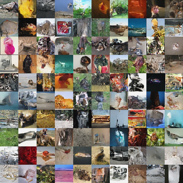
Figure 7: Samples from a model trained on Imagenet ($64\times 64$).

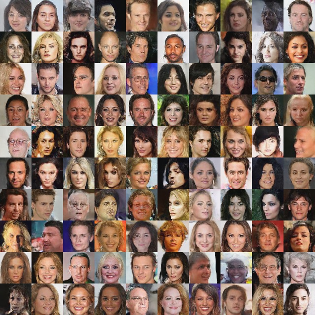
Figure 8: Samples from a model trained on CelebA.

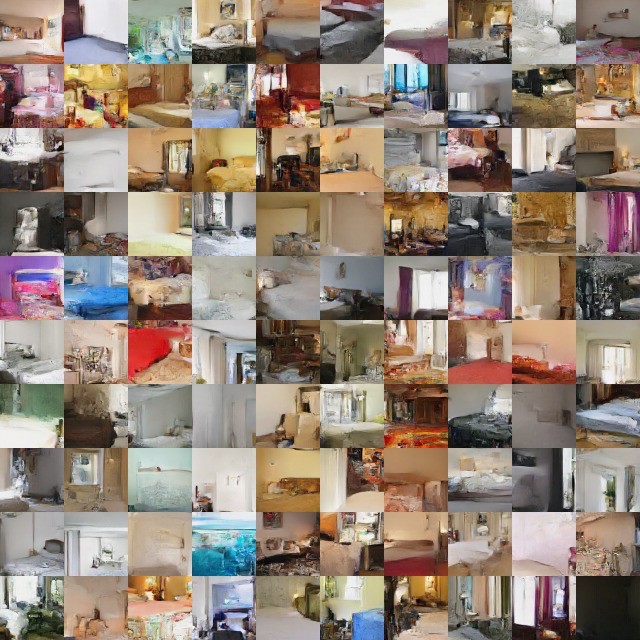
Figure 9: Samples from a model trained on LSUN (bedroom category).

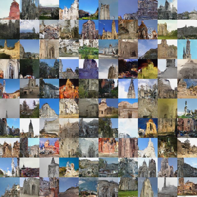
Figure 10: Samples from a model trained on LSUN (church outdoor category).

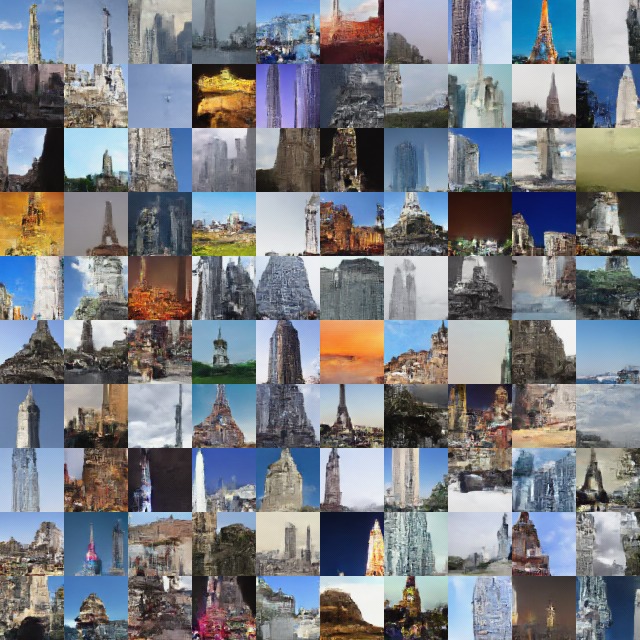
Figure 11: Samples from a model trained on LSUN (tower category).

Appendix B Manifold

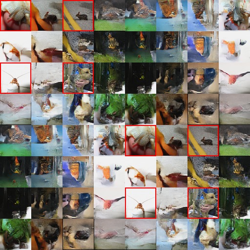
Figure 12: Manifold from a model trained on Imagenet ($64\times 64$). Images with red borders are taken from the validation set, and define the manifold. The manifold was computed as described in Equation 21, where the x-axis corresponds to $\phi$, and the y-axis to $\phi^{\prime}$, and where $\phi,\phi^{\prime}\in\{0,\frac{\pi}{4},\cdots,\frac{7\pi}{4}\}$.

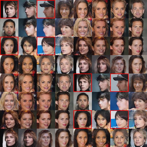
Figure 13: Manifold from a model trained on CelebA. Images with red borders are taken from the training set, and define the manifold. The manifold was computed as described in Equation 21, where the x-axis corresponds to $\phi$, and the y-axis to $\phi^{\prime}$, and where $\phi,\phi^{\prime}\in\{0,\frac{\pi}{4},\cdots,\frac{7\pi}{4}\}$.

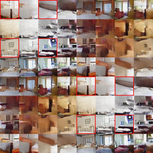
Figure 14: Manifold from a model trained on LSUN (bedroom category). Images with red borders are taken from the validation set, and define the manifold. The manifold was computed as described in Equation 21, where the x-axis corresponds to $\phi$, and the y-axis to $\phi^{\prime}$, and where $\phi,\phi^{\prime}\in\{0,\frac{\pi}{4},\cdots,\frac{7\pi}{4}\}$.

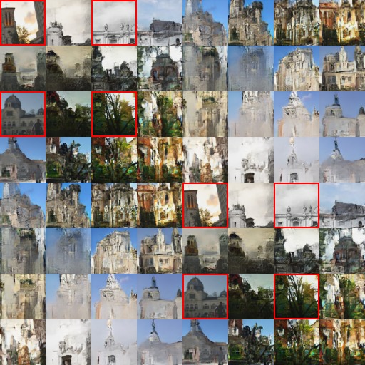
Figure 15: Manifold from a model trained on LSUN (church outdoor category). Images with red borders are taken from the validation set, and define the manifold. The manifold was computed as described in Equation 21, where the x-axis corresponds to $\phi$, and the y-axis to $\phi^{\prime}$, and where $\phi,\phi^{\prime}\in\{0,\frac{\pi}{4},\cdots,\frac{7\pi}{4}\}$.

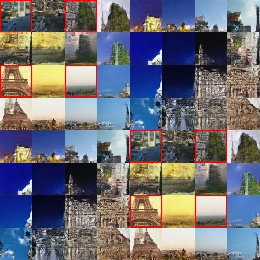
Figure 16: Manifold from a model trained on LSUN (tower category). Images with red borders are taken from the validation set, and define the manifold. The manifold was computed as described in Equation 21, where the x-axis corresponds to $\phi$, and the y-axis to $\phi^{\prime}$, and where $\phi,\phi^{\prime}\in\{0,\frac{\pi}{4},\cdots,\frac{7\pi}{4}\}$.

Appendix C Extrapolation

Inspired by the texture generation work by [19, 61] and extrapolation test with DCGAN [47], we also evaluate the statistics captured by our model by generating images twice or ten times as large as present in the dataset. As we can observe in the following figures, our model seems to successfully create a “texture” representation of the dataset while maintaining a spatial smoothness through the image. Our convolutional architecture is only aware of the position of considered pixel through edge effects in convolutions, therefore our model is similar to a stationary process. This also explains why these samples are more consistent in LSUN, where the training data was obtained using random crops.

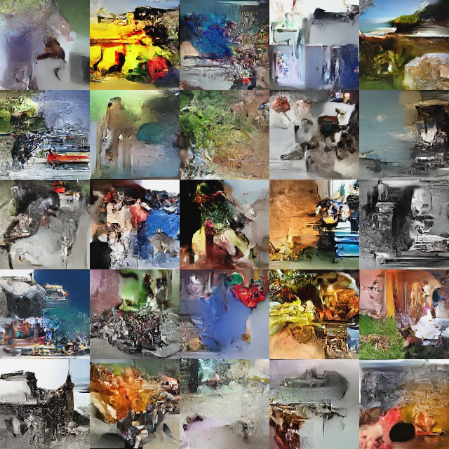
(a) $\times 2$

(b) $\times 10$

Figure 17: We generate samples a factor bigger than the training set image size on Imagenet ($64\times 64$).

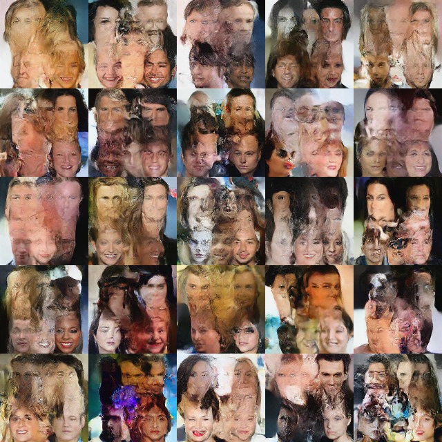
(a) $\times 2$

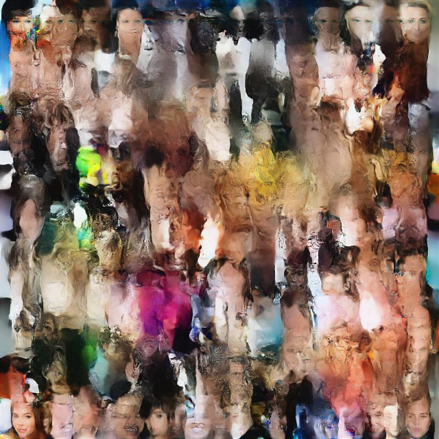
(b) $\times 10$

Figure 18: We generate samples a factor bigger than the training set image size on CelebA.

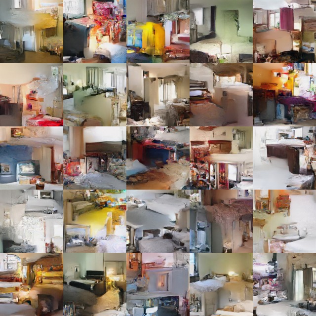
(a) $\times 2$

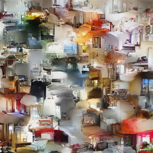
(b) $\times 10$

Figure 19: We generate samples a factor bigger than the training set image size on LSUN (bedroom category).

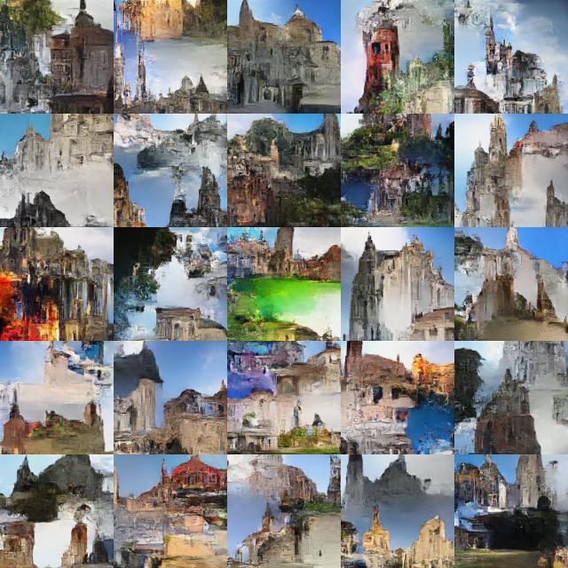
(a) $\times 2$

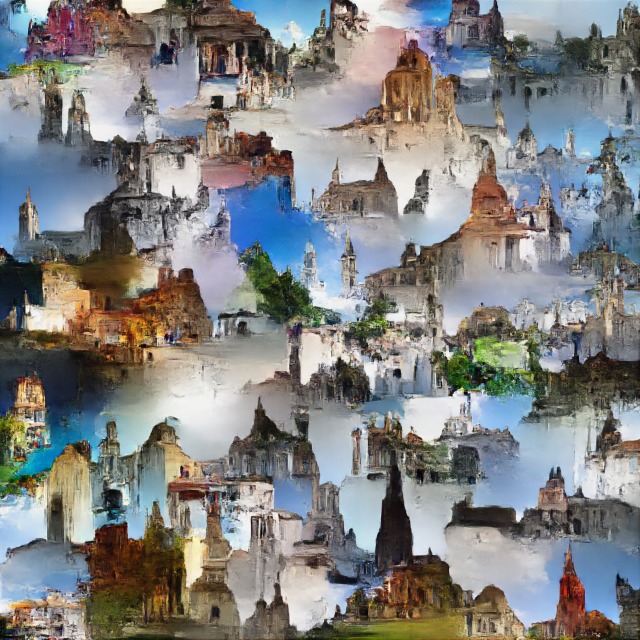
(b) $\times 10$

Figure 20: We generate samples a factor bigger than the training set image size on LSUN (church outdoor category).

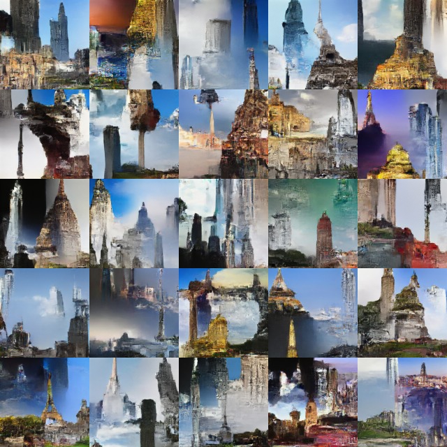
(a) $\times 2$

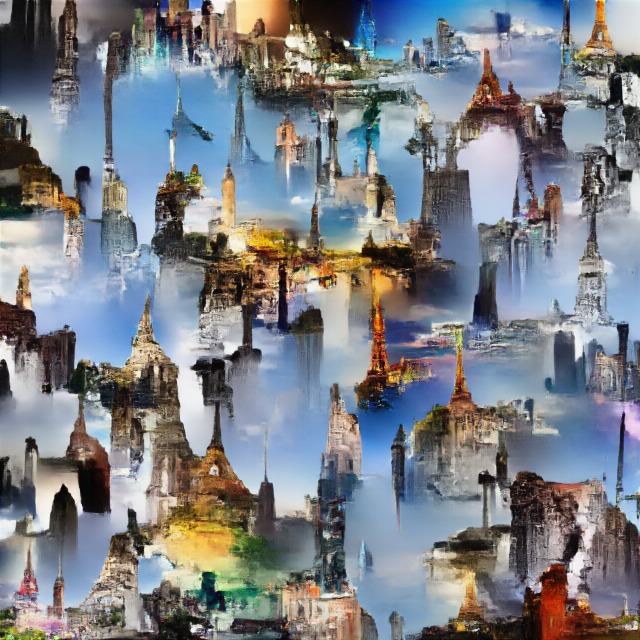
(b) $\times 10$

Figure 21: We generate samples a factor bigger than the training set image size on LSUN (tower category).

Appendix D Latent variables semantic

As in [22], we further try to grasp the semantic of our learned layers latent variables by doing ablation tests. We infer the latent variables and resample the lowest levels of latent variables from a standard gaussian, increasing the highest level affected by this resampling. As we can see in the following figures, the semantic of our latent space seems to be more on a graphic level rather than higher level concept. Although the heavy use of convolution improves learning by exploiting image prior knowledge, it is also likely to be responsible for this limitation.

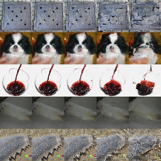
Figure 22: Conceptual compression from a model trained on Imagenet ($64\times 64$). The leftmost column represent the original image, the subsequent columns were obtained by storing higher level latent variables and resampling the others, storing less and less as we go right. From left to right: $100\%$, $50\%$, $25\%$, $12.5\%$ and $6.25\%$ of the latent variables are kept.

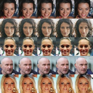
Figure 23: Conceptual compression from a model trained on CelebA. The leftmost column represent the original image, the subsequent columns were obtained by storing higher level latent variables and resampling the others, storing less and less as we go right. From left to right: $100\%$, $50\%$, $25\%$, $12.5\%$ and $6.25\%$ of the latent variables are kept.

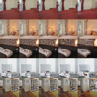
Figure 24: Conceptual compression from a model trained on LSUN (bedroom category). The leftmost column represent the original image, the subsequent columns were obtained by storing higher level latent variables and resampling the others, storing less and less as we go right. From left to right: $100\%$, $50\%$, $25\%$, $12.5\%$ and $6.25\%$ of the latent variables are kept.

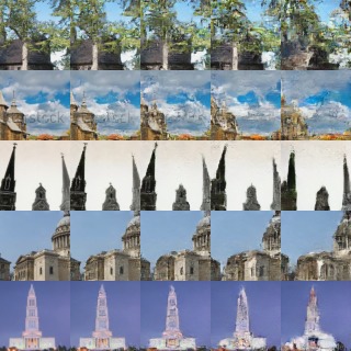
Figure 25: Conceptual compression from a model trained on LSUN (church outdoor category). The leftmost column represent the original image, the subsequent columns were obtained by storing higher level latent variables and resampling the others, storing less and less as we go right. From left to right: $100\%$, $50\%$, $25\%$, $12.5\%$ and $6.25\%$ of the latent variables are kept.

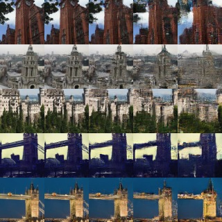
Figure 26: Conceptual compression from a model trained on LSUN (tower category). The leftmost column represent the original image, the subsequent columns were obtained by storing higher level latent variables and resampling the others, storing less and less as we go right. From left to right: $100\%$, $50\%$, $25\%$, $12.5\%$ and $6.25\%$ of the latent variables are kept.

Appendix E Batch normalization

We further experimented with batch normalization by using a weighted average of a moving average of the layer statistics $\tilde{\mu}_{t},\tilde{\sigma}^{2}_{t}$ and the current batch batch statistics $\hat{\mu}_{t},\hat{\sigma}_{t}^{2}$,

$$\tilde{\mu}_{t+1} =\rho\tilde{\mu}_{t}+(1-\rho)\hat{\mu}_{t}$$ (22)

$$\tilde{\sigma}^{2}_{t+1} =\rho\tilde{\sigma}^{2}_{t}+(1-\rho)\hat{\sigma}^{2}_{t},$$ (23)

where $\rho$ is the momentum. When using $\tilde{\mu}_{t+1},\tilde{\sigma}_{t+1}^{2}$, we only propagate gradient through the current batch statistics $\hat{\mu}_{t},\hat{\sigma}_{t}^{2}$. We observe that using this lag helps the model train with very small minibatches.

We used batch normalization with a moving average for our results on CIFAR-10.

Appendix F Attribute change

Additionally, we exploit the attribute information $y$ in CelebA to build a conditional model, i.e. the invertible function $f$ from image to latent variable uses the labels in $y$ to define its parameters. In order to observe the information stored in the latent variables, we choose to encode a batch of images $x$ with their original attribute $y$ and decode them using a new set of attributes $y^{\prime}$, build by shuffling the original attributes inside the batch. We obtain the new images $x^{\prime}=g\big{(}f(x;y);y^{\prime}\big{)}$.

We observe that, although the faces are changed as to respect the new attributes, several properties remain unchanged like position and background.

Figure 27: Examples $x$ from the CelebA dataset.

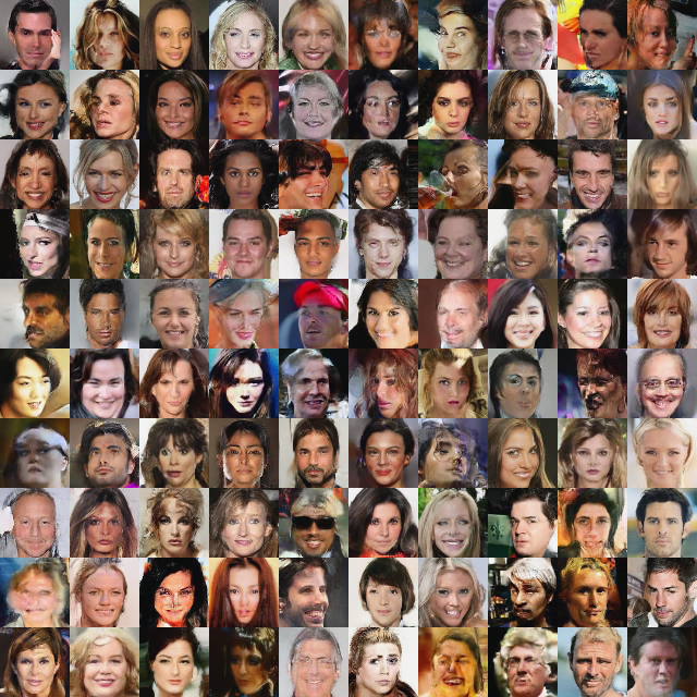
Figure 28: From a model trained on pairs of images and attributes from the CelebA dataset, we encode a batch of images with their original attributes before decoding them with a new set of attributes. We notice that the new images often share similar characteristics with those in Fig 27, including position and background.

References

- [1] Martın Abadi, Ashish Agarwal, Paul Barham, Eugene Brevdo, Zhifeng Chen, Craig Citro, Greg S Corrado, Andy Davis, Jeffrey Dean, Matthieu Devin, et al. Tensorflow: Large-scale machine learning on heterogeneous distributed systems. arXiv preprint arXiv:1603.04467, 2016.
- [2] Vijay Badrinarayanan, Bamdev Mishra, and Roberto Cipolla. Understanding symmetries in deep networks. arXiv preprint arXiv:1511.01029, 2015.
- [3] Johannes Ballé, Valero Laparra, and Eero P Simoncelli. Density modeling of images using a generalized normalization transformation. arXiv preprint arXiv:1511.06281, 2015.
- [4] Anthony J Bell and Terrence J Sejnowski. An information-maximization approach to blind separation and blind deconvolution. Neural computation, 7(6):1129–1159, 1995.
- [5] Yoshua Bengio. Artificial neural networks and their application to sequence recognition. 1991.
- [6] Yoshua Bengio and Samy Bengio. Modeling high-dimensional discrete data with multi-layer neural networks. In NIPS, volume 99, pages 400–406, 1999.
- [7] Mathias Berglund and Tapani Raiko. Stochastic gradient estimate variance in contrastive divergence and persistent contrastive divergence. arXiv preprint arXiv:1312.6002, 2013.
- [8] Samuel R Bowman, Luke Vilnis, Oriol Vinyals, Andrew M Dai, Rafal Jozefowicz, and Samy Bengio. Generating sentences from a continuous space. arXiv preprint arXiv:1511.06349, 2015.
- [9] Joan Bruna, Pablo Sprechmann, and Yann LeCun. Super-resolution with deep convolutional sufficient statistics. arXiv preprint arXiv:1511.05666, 2015.
- [10] Yuri Burda, Roger Grosse, and Ruslan Salakhutdinov. Importance weighted autoencoders. arXiv preprint arXiv:1509.00519, 2015.
- [11] Scott Shaobing Chen and Ramesh A Gopinath. Gaussianization. In Advances in Neural Information Processing Systems, 2000.
- [12] Junyoung Chung, Kyle Kastner, Laurent Dinh, Kratarth Goel, Aaron C Courville, and Yoshua Bengio. A recurrent latent variable model for sequential data. In Advances in neural information processing systems, pages 2962–2970, 2015.
- [13] Peter Dayan, Geoffrey E Hinton, Radford M Neal, and Richard S Zemel. The helmholtz machine. Neural computation, 7(5):889–904, 1995.
- [14] Gustavo Deco and Wilfried Brauer. Higher order statistical decorrelation without information loss. In G. Tesauro, D. S. Touretzky, and T. K. Leen, editors, Advances in Neural Information Processing Systems 7, pages 247–254. MIT Press, 1995.
- [15] Emily L. Denton, Soumith Chintala, Arthur Szlam, and Rob Fergus. Deep generative image models using a laplacian pyramid of adversarial networks. In Advances in Neural Information Processing Systems 28: Annual Conference on Neural Information Processing Systems 2015, December 7-12, 2015, Montreal, Quebec, Canada, pages 1486–1494, 2015.
- [16] Luc Devroye. Sample-based non-uniform random variate generation. In Proceedings of the 18th conference on Winter simulation, pages 260–265. ACM, 1986.
- [17] Laurent Dinh, David Krueger, and Yoshua Bengio. Nice: non-linear independent components estimation. arXiv preprint arXiv:1410.8516, 2014.
- [18] Brendan J Frey. Graphical models for machine learning and digital communication. MIT press, 1998.
- [19] Leon A. Gatys, Alexander S. Ecker, and Matthias Bethge. Texture synthesis using convolutional neural networks. In Advances in Neural Information Processing Systems 28: Annual Conference on Neural Information Processing Systems 2015, December 7-12, 2015, Montreal, Quebec, Canada, pages 262–270, 2015.
- [20] Mathieu Germain, Karol Gregor, Iain Murray, and Hugo Larochelle. MADE: masked autoencoder for distribution estimation. CoRR, abs/1502.03509, 2015.
- [21] Ian J. Goodfellow, Jean Pouget-Abadie, Mehdi Mirza, Bing Xu, David Warde-Farley, Sherjil Ozair, Aaron C. Courville, and Yoshua Bengio. Generative adversarial nets. In Advances in Neural Information Processing Systems 27: Annual Conference on Neural Information Processing Systems 2014, December 8-13 2014, Montreal, Quebec, Canada, pages 2672–2680, 2014.
- [22] Karol Gregor, Frederic Besse, Danilo Jimenez Rezende, Ivo Danihelka, and Daan Wierstra. Towards conceptual compression. arXiv preprint arXiv:1604.08772, 2016.
- [23] Shixiang Gu, Timothy Lillicrap, Ilya Sutskever, and Sergey Levine. Continuous deep q-learning with model-based acceleration. arXiv preprint arXiv:1603.00748, 2016.
- [24] Kaiming He, Xiangyu Zhang, Shaoqing Ren, and Jian Sun. Deep residual learning for image recognition. CoRR, abs/1512.03385, 2015.
- [25] Kaiming He, Xiangyu Zhang, Shaoqing Ren, and Jian Sun. Identity mappings in deep residual networks. CoRR, abs/1603.05027, 2016.
- [26] Sepp Hochreiter and Jürgen Schmidhuber. Long short-term memory. Neural Computation, 9(8):1735–1780, 1997.
- [27] Matthew D Hoffman, David M Blei, Chong Wang, and John Paisley. Stochastic variational inference. The Journal of Machine Learning Research, 14(1):1303–1347, 2013.
- [28] Aapo Hyvärinen, Juha Karhunen, and Erkki Oja. Independent component analysis, volume 46. John Wiley & Sons, 2004.
- [29] Aapo Hyvärinen and Petteri Pajunen. Nonlinear independent component analysis: Existence and uniqueness results. Neural Networks, 12(3):429–439, 1999.
- [30] Daniel Jiwoong Im, Chris Dongjoo Kim, Hui Jiang, and Roland Memisevic. Generating images with recurrent adversarial networks. arXiv preprint arXiv:1602.05110, 2016.
- [31] Sergey Ioffe and Christian Szegedy. Batch normalization: Accelerating deep network training by reducing internal covariate shift. arXiv preprint arXiv:1502.03167, 2015.
- [32] Rafal Józefowicz, Oriol Vinyals, Mike Schuster, Noam Shazeer, and Yonghui Wu. Exploring the limits of language modeling. CoRR, abs/1602.02410, 2016.
- [33] Diederik Kingma and Jimmy Ba. Adam: A method for stochastic optimization. arXiv preprint arXiv:1412.6980, 2014.
- [34] Diederik P Kingma, Tim Salimans, and Max Welling. Improving variational inference with inverse autoregressive flow. arXiv preprint arXiv:1606.04934, 2016.
- [35] Diederik P Kingma and Max Welling. Auto-encoding variational bayes. arXiv preprint arXiv:1312.6114, 2013.
- [36] Alex Krizhevsky and Geoffrey Hinton. Learning multiple layers of features from tiny images, 2009.
- [37] Hugo Larochelle and Iain Murray. The neural autoregressive distribution estimator. In AISTATS, 2011.
- [38] Anders Boesen Lindbo Larsen, Søren Kaae Sønderby, and Ole Winther. Autoencoding beyond pixels using a learned similarity metric. CoRR, abs/1512.09300, 2015.
- [39] Yann A LeCun, Léon Bottou, Genevieve B Orr, and Klaus-Robert Müller. Efficient backprop. In Neural networks: Tricks of the trade, pages 9–48. Springer, 2012.
- [40] Chen-Yu Lee, Saining Xie, Patrick Gallagher, Zhengyou Zhang, and Zhuowen Tu. Deeply-supervised nets. arXiv preprint arXiv:1409.5185, 2014.
- [41] Ziwei Liu, Ping Luo, Xiaogang Wang, and Xiaoou Tang. Deep learning face attributes in the wild. In Proceedings of International Conference on Computer Vision (ICCV), December 2015.
- [42] Lars Maaløe, Casper Kaae Sønderby, Søren Kaae Sønderby, and Ole Winther. Auxiliary deep generative models. arXiv preprint arXiv:1602.05473, 2016.
- [43] Andriy Mnih and Karol Gregor. Neural variational inference and learning in belief networks. arXiv preprint arXiv:1402.0030, 2014.
- [44] Volodymyr Mnih, Koray Kavukcuoglu, David Silver, Andrei A Rusu, Joel Veness, Marc G Bellemare, Alex Graves, Martin Riedmiller, Andreas K Fidjeland, Georg Ostrovski, et al. Human-level control through deep reinforcement learning. Nature, 518(7540):529–533, 2015.
- [45] Radford M Neal and Geoffrey E Hinton. A view of the em algorithm that justifies incremental, sparse, and other variants. In Learning in graphical models, pages 355–368. Springer, 1998.
- [46] Aaron van den Oord, Nal Kalchbrenner, and Koray Kavukcuoglu. Pixel recurrent neural networks. arXiv preprint arXiv:1601.06759, 2016.
- [47] Alec Radford, Luke Metz, and Soumith Chintala. Unsupervised representation learning with deep convolutional generative adversarial networks. CoRR, abs/1511.06434, 2015.
- [48] Danilo Jimenez Rezende and Shakir Mohamed. Variational inference with normalizing flows. arXiv preprint arXiv:1505.05770, 2015.
- [49] Danilo Jimenez Rezende, Shakir Mohamed, and Daan Wierstra. Stochastic backpropagation and approximate inference in deep generative models. arXiv preprint arXiv:1401.4082, 2014.
- [50] Oren Rippel and Ryan Prescott Adams. High-dimensional probability estimation with deep density models. arXiv preprint arXiv:1302.5125, 2013.
- [51] David E Rumelhart, Geoffrey E Hinton, and Ronald J Williams. Learning representations by back-propagating errors. Cognitive modeling, 5(3):1, 1988.
- [52] Olga Russakovsky, Jia Deng, Hao Su, Jonathan Krause, Sanjeev Satheesh, Sean Ma, Zhiheng Huang, Andrej Karpathy, Aditya Khosla, Michael Bernstein, et al. Imagenet large scale visual recognition challenge. International Journal of Computer Vision, 115(3):211–252, 2015.
- [53] Ruslan Salakhutdinov and Geoffrey E Hinton. Deep boltzmann machines. In International conference on artificial intelligence and statistics, pages 448–455, 2009.
- [54] Tim Salimans and Diederik P Kingma. Weight normalization: A simple reparameterization to accelerate training of deep neural networks. arXiv preprint arXiv:1602.07868, 2016.
- [55] Tim Salimans, Diederik P Kingma, and Max Welling. Markov chain monte carlo and variational inference: Bridging the gap. arXiv preprint arXiv:1410.6460, 2014.
- [56] Lawrence K Saul, Tommi Jaakkola, and Michael I Jordan. Mean field theory for sigmoid belief networks. Journal of artificial intelligence research, 4(1):61–76, 1996.
- [57] Karen Simonyan and Andrew Zisserman. Very deep convolutional networks for large-scale image recognition. arXiv preprint arXiv:1409.1556, 2014.
- [58] Paul Smolensky. Information processing in dynamical systems: Foundations of harmony theory. Technical report, DTIC Document, 1986.
- [59] Jascha Sohl-Dickstein, Eric A. Weiss, Niru Maheswaranathan, and Surya Ganguli. Deep unsupervised learning using nonequilibrium thermodynamics. In Proceedings of the 32nd International Conference on Machine Learning, ICML 2015, Lille, France, 6-11 July 2015, pages 2256–2265, 2015.
- [60] Sasha Targ, Diogo Almeida, and Kevin Lyman. Resnet in resnet: Generalizing residual architectures. CoRR, abs/1603.08029, 2016.
- [61] Lucas Theis and Matthias Bethge. Generative image modeling using spatial lstms. In Advances in Neural Information Processing Systems, pages 1918–1926, 2015.
- [62] Lucas Theis, Aäron Van Den Oord, and Matthias Bethge. A note on the evaluation of generative models. CoRR, abs/1511.01844, 2015.
- [63] Dustin Tran, Rajesh Ranganath, and David M Blei. Variational gaussian process. arXiv preprint arXiv:1511.06499, 2015.
- [64] Benigno Uria, Iain Murray, and Hugo Larochelle. Rnade: The real-valued neural autoregressive density-estimator. In Advances in Neural Information Processing Systems, pages 2175–2183, 2013.
- [65] Hado van Hasselt, Arthur Guez, Matteo Hessel, and David Silver. Learning functions across many orders of magnitudes. arXiv preprint arXiv:1602.07714, 2016.
- [66] Oriol Vinyals, Samy Bengio, and Manjunath Kudlur. Order matters: Sequence to sequence for sets. arXiv preprint arXiv:1511.06391, 2015.
- [67] Manuel Watter, Jost Springenberg, Joschka Boedecker, and Martin Riedmiller. Embed to control: A locally linear latent dynamics model for control from raw images. In Advances in Neural Information Processing Systems, pages 2728–2736, 2015.
- [68] Ronald J Williams. Simple statistical gradient-following algorithms for connectionist reinforcement learning. Machine learning, 8(3-4):229–256, 1992.
- [69] Fisher Yu and Vladlen Koltun. Multi-scale context aggregation by dilated convolutions. arXiv preprint arXiv:1511.07122, 2015.
- [70] Fisher Yu, Yinda Zhang, Shuran Song, Ari Seff, and Jianxiong Xiao. Construction of a large-scale image dataset using deep learning with humans in the loop. arXiv preprint arXiv:1506.03365, 2015.
- [71] Richard Zhang, Phillip Isola, and Alexei A Efros. Colorful image colorization. arXiv preprint arXiv:1603.08511, 2016.