Observations of metals in the z$\,\approx\,$3.5 intergalactic medium and comparison to the EAGLE simulations

Abstract

We study the $z\approx 3.5$ intergalactic medium (IGM) by comparing new, high-quality absorption spectra of eight QSOs with $\langle z_{\text{QSO}}\rangle=3.75$, to virtual observations of the EAGLE cosmological hydrodynamical simulations. We employ the pixel optical depth method and uncover strong correlations between various combinations of Hi, Ciii, Civ, Siiii, Siiv, and Ovi. We find good agreement between many of the simulated and observed correlations, including $\tau_{\rm O\textsc{vi}}(\tau_{\rm H\textsc{i}})$. However, the observed median optical depths for the $\tau_{\rm C\textsc{iv}}(\tau_{\rm H\textsc{i}})$ and $\tau_{\rm Si\textsc{iv}}(\tau_{\rm H\textsc{i}})$ relations are higher than those measured from the mock spectra. The discrepancy increases from up to $\approx 0.1$ dex at $\tau_{\rm H\textsc{i}}=1$ to $\approx 1$ dex at $\tau_{\rm H\textsc{i}}=10^{2}$, where we are likely probing dense regions at small galactocentric distances. As possible solutions, we invoke (a) models of ionizing radiation softened above 4 Ryd to account for delayed completion of Heii reionization; (b) simulations run at higher resolution; (c) the inclusion of additional line broadening due to unresolved turbulence; and (d) increased elemental abundances; however, none of these factors can fully explain the observed differences. Enhanced photoionization of Hi by local sources, which was not modelled, could offer a solution. However, the much better agreement with the observed Ovi(Hi) relation, which we find probes a hot and likely collisionally ionized gas phase, indicates that the simulations are not in tension with the hot phase of the IGM, and suggests that the simulated outflows may entrain insufficient cool gas.

1 Introduction

It is now well established that the high redshift intergalactic medium (IGM) is enriched with heavy metals to metallicites of $10^{-3}$ to $10^{-2}$ ${\rm Z}_{\odot}$ (e.g., Cowie et al., 1995; Schaye et al., 2003; Simcoe et al., 2004; Aguirre et al., 2008). While metals only constitute a fraction of the total baryon budget, they play an integral role in our understanding of galaxy formation and evolution by providing a fossil record of star formation, and by impacting upon cooling-rates which can alter structure on many scales (e.g., Haas et al., 2013).

Metals are synthesized in and released from stars located in very overdense environments, therefore they need to travel large distances to reach the diffuse IGM, and this transport is likely driven by feedback from star formation and active galactic nuclei (AGN). Simulations have shown that metal pollution by galactic winds yields reasonable enrichment statistics, without destroying the filamentary pattern that gives rise to the Hi Ly$\alpha$ forest (Theuns et al., 2002). Although the need for inclusion of these processes is clear, the mechanisms responsible are not resolved, even in state-of-the-art cosmological simulations, making their implementation uncertain. By comparing observed and theoretical metal-line absorption in the IGM, we may be able to constrain enrichment mechanisms such as outflows.

Models and simulations of the IGM have been used to make predictions about sources of metal pollution. Booth et al. (2012) established that the observations of Schaye et al. (2003) of Civ associated with weak Hi at $z\approx 3$ can only be explained if the low-density IGM was enriched primarily by low-mass galaxies ($M_{\text{halo}}\leq 10^{10}$ M_⊙) that drive outflows to distances of $\sim 10^{2}$ proper kiloparsecs (pkpc), and calculated that $>10$% of the simulated volume and $>50$% of the baryonic mass in their successful model was polluted by metals. The simulations studied by Wiersma et al. (2010) indicate that at least half of the metals found in the $z=2$ IGM were ejected from galaxies at $z\geq 3$, and that the haloes hosting these galaxies had masses less than $M_{\text{halo}}=10^{11}$ M_⊙. This picture is consistent with that inferred from observations by Simcoe et al. (2004), who estimate that half of all baryons are enriched to metallities $>10^{-3.5}$ Z_⊙ by $z\sim 2.5$.

Studies of the IGM using the direct detection of individual metal lines can typically probe only relatively overdense gas, which constitutes a very small volume fraction of the Universe. In this work, we employ an approach known as the pixel optical depth method (Cowie & Songaila, 1998; Ellison et al., 2000; Schaye et al., 2000b; Aguirre et al., 2002; Schaye et al., 2003; Turner et al., 2014), and provide a public version of the code at https://github.com/turnerm/podpy. This technique is a valuable tool for studying the IGM, as it enables us to detect metals statistically even in low-density gas. At the redshifts studied in this work, direct detection of metal-line absorption in regions of the spectrum contaminated by Hi is nearly impossible due to the density of the forest of absorption features. By using the pixel optical depth method, we can correct for contamination and derive statistical properties of the absorption by metals in this region. In this work we take advantage of the fact that this technique is fast and objective, and can be applied uniformly to both observations and simulations.

Our observational sample consists of new spectra of eight $3.62\leq z\leq 3.92$ QSOs with uniform coverage and high signal-to-noise (S/N). We compare the results to the Evolution and Assembly of Galaxies and their Environments (EAGLE) cosmological hydrodynamical simulations (Schaye et al., 2015; Crain et al., 2015). The EAGLE simulations are ideal for studying metal-line absorption in the IGM, as they have been run at relatively high resolution in a cosmologically representative volume ($2\times 1504^{3}$ particles in a 100 cMpc box). The fiducial EAGLE model is able to reproduce the present-day galaxy stellar mass function, galaxy sizes and the Tully Fisher relation (Schaye et al., 2015), and has been found to match observations of galaxy colours (Trayford et al., 2015) and the evolution of galaxy stellar masses (Furlong et al., 2015b) and sizes (Furlong et al., 2015a). Furthermore, the simulations are in good agreement with a number of relevant observables, including the properties of Hi absorption at $z\sim 2$–$3$ (Rahmati et al., 2015), as well as the Ovi and Civ  (Schaye et al., 2015) and the Hi (Crain et al., 2016) column density distribution functions (CDDFs) at $z\sim 0$ (although for the latter we note that a higher than fiducial resolution is needed to achieve agreement).

Rahmati et al. (2016) compared observed metal-line CDDFs for various ions and redshifts with the predictions from EAGLE, finding generally good agreement. Their study also included CIV, which was compared to the observations of Songaila (2005, $z=1.5\text{--}5.5$), D’Odorico et al. (2010, $z=1.5\text{--}4.0$), and Boksenberg & Sargent (2015, $z=1.6\text{--}4.4$). Although the redshift ranges of these surveys overlap with ours, they are much wider and hence likely affected by evolutionary trends. These observational studies each used different, subjective methods to decompose the absorption into Voigt profiles, which limits their utility for testing models. Indeed, the different studies do not agree with each other, making it relatively easy for a single model to agree with the data. Here we will instead employ a like-for-like comparison of new data with virtual EAGLE observations tailored to mimic the characteristics of our own quasar spectra and analysed using the same automated method. We will consider relations between the pixel optical depths of Hi, Ciii, Civ, Siiii, Siiv and Ovi.

This paper is structured as follows. In § 2, we describe the observations and simulations. We also summarize the pixel optical depth method, and how it is applied. The results are presented in § 3, and we give a discussion and conclusions in § 4 and 5, respectively. Throughout this work, we denote proper and comoving distances as pMpc and cMpc, respectively. Both simulations and observations use cosmological parameters determined from the Planck mission (Planck Collaboration et al., 2014), i.e. $H_{\rm 0}=67.8$ km s^-1 Mpc^-1, $\Omega_{\rm m}=0.307$, and $\Omega_{\Lambda}=0.693$.

2 Method

2.1 Observations

We analyze a sample of eight QSOs with $3.62\leq z_{\text{QSO}}\leq 3.922$. They were selected based on their redshift and the existence of substantial, high S/N data taken with VLT/UVES. Initially, there were already 76.0 hours of UVES data, excluding overheads, of the QSOs. Follow-up observations to fill in the gaps and improve S/N were completed in 62.7 hours of on-source time in programmes 091.A-0833, 092.A-0011 and 093.A-0575 (P.I. Schaye). We note that for Q1422$+$23, the gaps in the UVES data were filled using archival observations with Keck/HIRES of comparable S/N and resolution (which is $\approx 8.5$ km s^-1). The properties of the QSOs and the S/N of the spectra are summarized in Table 1.

The reduction of the UVES data was performed using the UVES_headsort and UVES_popler software by Michael T. Murphy, and binned to have a uniform velocity dispersion of 1.3 km s^-1. The HIRES data was reduced using T. Barlow’s MAKEE package, and binned on to 2.8 km s^-1 pixels. The continuum fits for the spectra were performed by hand by M. Turner. Any DLAs or Lyman break regions (i.e., due to strong absorbers in Hi) were masked out, with the exception of DLAs in the Ly$\alpha$ forest, which were unmasked when recovering the Hi to be used for subtraction of contaminating absorption by higher-order Lyman series lines from Ovi and Ciii optical depths.

To homogenize the continuum fitting errors, we implemented the automated sigma-clipping procedure of Schaye et al. (2003) at wavelengths greater than that of the QSO’s Ly$\alpha$ emission, which was applied to both the observed and simulated spectra. The spectrum is divided into rest-frame bins of $\Delta\lambda=20$ Å, which have central wavelength $\lambda_{i}$ and median flux $\bar{f_{i}}$. A B-spline of order 3 is then interpolated through all $\bar{f_{i}}$ values, and any pixels with flux $N_{\sigma}^{\rm cf}\times\sigma$ below the interpolated values are discarded, where $\sigma$ is the normalized noise array. We then recalculate $\bar{f_{i}}$ without the discarded pixels, and repeat the procedure until convergence is reached. We use $N_{\sigma}^{\rm cf}=2$, which has been shown to be optimal in the Civ region for spectra with a quality similar to ours, as it induces errors that are smaller than the noise by at least an order of magnitude (Schaye et al., 2003).

Table 1: Properties of the QSOs used in this work, and the median S/N in the Hi Ly$\alpha$ and Civ recovery regions. The columns list, from left to right, name, right ascension, declination, redshift, magnitude and magnitude band (either $V$-band (V), $R$-band (R), or photographic (P)) from Véron-Cetty & Véron (2010), median signal-to-noise in the Ly$\alpha$ forest region and Civ region, respectively (see § 2.3 for the definition of these regions), the median optical depth of Hi in the Ly$\alpha$ forest, the factor $C_{\rm UVB}$ used to scale the UVB in the simulations, and the redshift midpoint of eq. 1 that defines the Ly$\alpha$ forest region.

Name	R.A.	Dec	$z_{\text{QSO}}$	Mag	Band	S/NLyα	S/N${}_{\rm C\textsc{iv}}$	$\log_{10}\tau^{\rm med}_{\rm H\textsc{i}}$	$C_{\rm UVB}$	$z^{\rm mid}_{{\rm Ly}\alpha}$
Q1422$+$23	14:24:38	+22:56:01	3.620	15.84	V	87	82	$-0.605$	0.896	3.24
Q0055$-$269	00:57:58	-26:43:14	3.655	17.47	P	60	79	$-0.583$	1.123	3.27
Q1317$-$0507	13:20:30	-18:36:25	3.700	18.10	P	59	90	$-0.549$	1.009	3.31
Q1621$-$0042	16:21:17	-23:17:10	3.709	17.97	V	78	92	$-0.546$	0.807	3.32
QB2000$-$330	20:03:24	-32:51:44	3.773	17.30	R	105	83	$-0.501$	0.809	3.38
PKS1937$-$101	19:39:57	-13:57:19	3.787	17.00	R	96	64	$-0.494$	1.293	3.39
J0124$+$0044	01:24:03	+00:44:32	3.834	18.71	V	48	59	$-0.445$	0.898	3.43
BRI1108$-$07	11:11:13	-15:55:58	3.922	18.10	R	29	29	$-0.390$	0.808	3.51

2.2 Simulations

We compare the observations to predictions from the EAGLE cosmological hydrodynamical simulations. EAGLE was run with a substantially modified version of the $N$-body TreePM smoothed particle hydrodynamics (SPH) code GADGET 3 (last described in Springel 2005). EAGLE uses the package of hydrodynamics updates “Anarchy” (Dalla Vecchia, in prep.; see Appendix A1 of Schaye et al. 2015) which invokes the pressure-entropy formulation of SPH from Hopkins (2013), the time-step limiter from Durier & Dalla Vecchia (2012), the artificial viscosity switch from Cullen & Dehnen (2010), an artificial conduction switch close to that of Price (2008), and the $C^{2}$ Wendland (1994) kernel. The influence of the updates is explored by Schaller et al. (2015). The fiducial EAGLE model is run in a 100 cMpc periodic box with $1504^{3}$ of both dark matter and baryonic particles, and is denoted Ref-L1001504. To test convergence with resolution and box size, runs varying the number of particles and box size were also conducted, and are listed in Table 2.

The stellar feedback in EAGLE is implemented as described by Dalla Vecchia & Schaye (2012), where thermal energy is injected stochastically. While the temperature of heated particles is always increased by $10^{7.5}$ K, the probability of heating varies with the local metallicity and density (Schaye et al., 2015; Crain et al., 2015). The simulations include thermal AGN feedback (Booth & Schaye, 2009), also implemented stochastically (Schaye et al., 2015). Both stellar and AGN feedback have been calibrated such that the simulations match the observed $z\sim 0$ stellar mass function and galaxy–black hole mass relation, and give sensible disc galaxy sizes. We note that of the two highest-resolution runs, Ref-L025N072 has been realized with the same subgrid parameters used in the fiducial model, while for the Recal-L025N072 the subgrid parameters were re-calibrated to better match the observed galaxy stellar mass function.

EAGLE also includes a subgrid model for photo-heating and radiative cooling via eleven elements: hydrogen, helium, carbon, nitrogen, oxygen, neon, magnesium, silicon, sulphur, calcium and iron (Wiersma et al., 2009a), assuming a Haardt & Madau (2001) UV and X-ray background. Star formation is implemented with a gas metallicity-dependent density threshold (Schaye, 2004) as described by Schaye & Dalla Vecchia (2008), followed by stellar evolution and enrichment from Wiersma et al. (2009b). Finally, details of the subgrid model for black hole seeding and growth can be found in Springel et al. (2005); Rosas-Guevara et al. (2015) and Schaye et al. (2015).

For each of our eight observed QSOs in Table 1, we synthesize 100 corresponding mock spectra using the SPECWIZARD package by Schaye, Booth, and Theuns (implemented as in Schaye et al. 2003, see also Appendix A4 of Theuns et al. 1998). To create mock spectra that resemble the observed QSOs and whose absorption features span a large redshift range, we follow Schaye et al. (2003) and stitch together the physical state of the gas intersecting uncorrelated sightlines from snapshots with different redshifts. The ionization balance of each gas particle is estimated using interpolation tables generated from Cloudy (Ferland et al., 2013, version 13.03) assuming uniform illumination by an ultra-violet background (UVB).

We take the QSO+galaxy Haardt & Madau (2001) UVB (denoted as “HM01”) to be our fiducial model, and have plotted the intensity as a function of energy at $z=3.5$ in Fig. 1. We also consider the Haardt & Madau (2001) background using quasars only (“Q-only”), which is much harder than the fiducial model above $\approx 4$ Ryd. Furthermore, to explore the possible effects of a delayed Heii reionization, we consider a UVB that is significantly softer above 4 Ryd. To implement this, we use the QSO+galaxy model and reduce the intensity above 4 Ryd by a factor of 100, which we denote as “4Ryd-100”.

Self-shielding for Hi was included by modifying the ionization fraction using the fitting functions of Rahmati et al. (2013a). The normalization of the UVB is set such that the median recovered Hi Ly$\alpha$ optical depth of the simulated QSOs agrees with that of the observations at the same redshift. A unique value of $C_{\rm UVB}$ is determined for each observed QSO and corresponding set of 100 mock spectra, and the values are presented in Table 1.

In the EAGLE simulations, the dense particles that represent the multiphase interstellar medium (ISM, $n_{\rm H}>0.1$ cm^-3) are not allowed to cool below an effective equation of state (EoS), and their temperature can be interpreted as a proxy for the pressure at which the warm and cool ISM phases equilibriate. We set their temperatures to $10^{4}$ K when generating the mock spectra, although we note that due to the small cross-section of such dense absorbers the effect of including them is negligible.

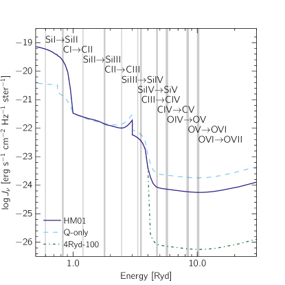
Figure 1: The intensity as a function of energy for the different UVB models. The different models are: HM01 QSO+galaxy (Haardt & Madau, 2001), which is our fiducial model; Q-only, which is also by Haardt & Madau (2001) but only considers an ionizing contribution from QSOs; and 4Ryd-100, the same as the fiducial model except that the intensity is reduced by a factor of 100 above 4 Ryd. The vertical light grey lines indicate the ionization energies of ions of interest, where increasing line thickness denotes silicon, carbon and oxygen ions, respectively. All of the UVBs have been normalized to have the same intensity as HM01 at 1 Ryd.

Each set of 100 mock spectra is synthesized to have redshifts identical to that of their corresponding observed QSO, and we consider absorption ranging from $1.5<z<z_{\text{QSO}}$ in every case. We include contributions from 31 Hi Lyman series transitions beginning with Ly$\alpha$, and metal-line absorption from Cii, Ciii, Civ, Feii, Nv, Ovi, Siii, Siiii, and Siiv (see Appendix A for the rest wavelengths and oscillator strengths of these transitions). To match the spectral properties of the observations, the simulated spectra are convolved with a Gaussian with a FWHM of 6.6 km s^-1, and resampled on to pixels of 1.3 km s^-1. For each observed QSO, we have measured the RMS noise in bins of 150 Å in wavelength and 0.2 in normalized flux. We then use these measurements to add random Gaussian noise with the same variance to the simulations.

Table 2: Characteristics of the EAGLE simulations. From left to right, the columns list the simulation name, box size, number of particles, initial baryonic particle mass, dark matter particle mass, comoving (Plummer-equivalent) gravitational softening, and maximum physical softening.

Simulation	$L$	$N$	$m_{\rm b}$	$m_{\rm dm}$	$\epsilon_{\rm com}$	$\epsilon_{\rm prop}$
	[cMpc]		[M⊙]	[M⊙]	[ckpc]	[pkpc]
Ref-L100N1504	100	$2\times 1504^{3}$	$1.81\times 10^{6}$	$9.70\times 10^{6}$	2.66	0.70
Ref-L050N0752	50	$2\times 752^{3}$	$1.81\times 10^{6}$	$9.70\times 10^{6}$	2.66	0.70
Ref-L025N0376	25	$2\times 376^{3}$	$1.81\times 10^{6}$	$9.70\times 10^{6}$	2.66	0.70
Ref-L025N0752	25	$2\times 752^{3}$	$2.26\times 10^{5}$	$1.21\times 10^{6}$	1.33	0.35
Recal-L025N0752	25	$2\times 752^{3}$	$2.26\times 10^{5}$	$1.21\times 10^{6}$	1.33	0.35

2.3 Analyzed redshift range

The first step for the pixel optical depth recovery involves choosing optimal redshift limits. The fiducial redshift range is selected to lie in the Ly$\alpha$ forest, defined to be:

$$(1+z_{\rm qso})\dfrac{\lambda_{{\rm Ly}\beta}}{\lambda_{{\rm Ly}\alpha}}-1\leq z\leq z_{\rm qso}-(1+z_{\rm qso})\dfrac{3000\,{\rm km~{}s}^{-1}}{c}$$ (1)

where $\lambda_{{\rm Ly}\alpha}=1215.7$ Å and $\lambda_{{\rm Ly}\beta}=1025.7$ Å are the Hi Ly$\alpha$ and Ly$\beta$ rest wavelengths, respectively. The lower limit was chosen to avoid the Ly$\beta$ forest and corresponds to the Ly$\beta$ transition at the redshift of the QSO, while the upper limit is 3000 km s^-1 bluewards of the QSO redshift to avoid any proximity effects.

For Hi, Civ ($\lambda_{\rm rest}=[1548.2,1550.8]$ Å) and Ciii ($\lambda_{\rm rest}=977.0$ Å) we use the above redshift limits. For the remaining ions, we make slight modifications, listed below, in order to homogenize the contamination. We use the notation $\lambda_{Z,k}$ to denote the rest wavelength of multiplet component $k$ of the ion $Z$.

1. Ovi ($\lambda_{\rm rest}=[1031.9,1037.6]$ Å): We limit the recovery to where Ovi overlaps with the Ly$\beta$ forest and place a cut-off at the Ly$\alpha$ forest region, which leads to $z_{\rm max}=(1+z_{\rm qso})\lambda_{\rm H\textsc{i},{\rm Ly}\beta}/\lambda_{\rm O\textsc{vi},2}-1$

2. Siiii ($\lambda_{\rm rest}=1206.6$ Å): We constrain the recovered optical depth region to not extend outside of the Ly$\alpha$ forest. For Siiii, which extends slightly bluewards into the Ly$\beta$ forest, we set $z_{\rm min}=(1+z_{\rm qso})\lambda_{{\rm Ly}\beta}/\lambda_{\rm Si\textsc{iii}}$.

3. Siiv ($\lambda_{\rm rest}=[1393.8,1402.8]$ Å): To avoid contamination by the Ly$\alpha$ forest, we limit the blue end of the Siiv recovery by setting $z_{\rm min}=(1+z_{\rm qso})\lambda_{{\rm Ly}\alpha}/\lambda_{\rm Si\textsc{iv},1}-1$.

2.4 Pixel optical depth method

We employ the pixel optical depth method, which we use to study absorption on an individual pixel basis rather than by fitting Voigt profiles to individual lines. The goal is to obtain statistics on absorption by Hi and various metal ions in the IGM, and on how their absorption relates to one another. Our implementation is close to that of Aguirre et al. (2002), but with the improvements of Turner et al. (2014), and the effects of varying the chosen parameters can be found in both works. The exact methodology is described in full detail in Appendix A of Turner et al. (2014), and is summarized below. A working version of the code can be found at https://github.com/turnerm/podpy.

After restricting the redshift range, the next step is to convert the flux of every pixel of ion $Z$ and multiplet component $k$ to an optical depth $\tau_{Z,k}(z)=-\ln(F)$, where $F(\lambda)$ is the normalised flux at $\lambda=\lambda_{k}(1+z)$. Then, depending on the ion, corrections are made for saturation or contamination, as described below.

1. For Hi Ly$\alpha$, while there is very little contamination in the Ly$\alpha$ forest, the absorption in many of the pixels will be saturated, and we use the higher order Lyman series transitions to correct for this. Specifically, if we consider a Ly$\alpha$ pixel to be saturated, we look to $N=16$ higher-order Lyman lines (beginning with Hi Ly$\beta$), and take the minimum optical depth, scaled to that of Ly$\alpha$, of all unsaturated pixels at the same redshift (if any). If we are unable to correct the pixel due to saturation of the higher-order transitions, we set it to $10^{4}$ (so that these pixels can still be used for computing the median). Finally, we search for and discard any contaminated pixels, by checking that higher-order transitions do not have optical depth values significantly below what would be expected from the scaled Hi Ly$\alpha$ optical depth.

2. For Ovi and Ciii, we can use the corrected Hi Ly$\alpha$ optical depths to estimate and subtract contamination by Hi. We do so beginning with Hi Ly$\beta$ ($N=2$) and use higher-order Lyman series orders up to $N=5$. For saturated Ovi and Ciii pixels, the optical depth is not well defined and therefore the above subtraction is not performed. Instead, we leave the pixel uncorrected, unless the saturation can be attributed to Hi, in which case the pixel is discarded.

3. Siiv and Ovi are both closely-spaced doublets, and we can use this fact to correct for contamination. To do so, we scale the optical depth of the weak component to match that of the strong component, and take the minimum of the two components modulo noise. We only take the scaled optical depth of the weaker component if it is significantly lower (when taking into account the noise array) than the stronger component.

4. For Civ, which is a strong transition redward of the Ly$\alpha$ forest, the largest source of contamination is by its own doublet. To correct for this, we perform an iterative self-contamination correction. We first discard any pixels determined to be contaminated by other ions, by checking whether the optical depth of a pixel is too high to be explained by half of the associated stronger component combined with twice the associated weaker component. We then subtract the estimated contribution of the weaker component from each pixel, iterating until convergence is reached.

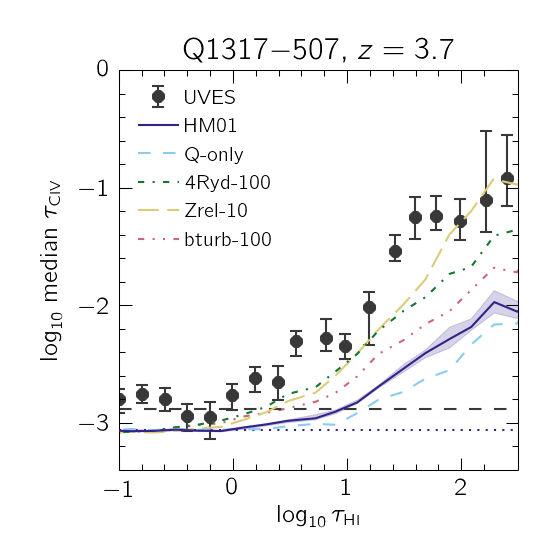
Figure 2: Example analysis of the Civ(Hi) relation for Q1317$-$507. The measured optical depths from the observations are shown by the points, and those recovered from the mock spectra are indicated by the curves, with the different colours and line styles representing variations in the model. $1\sigma$ errors are indicated by the bars (shaded region) for the observations (fiducial simulation), and were determined by bootstrap resampling spectral chunks (mock spectra). We indicate $\tau_{\text{min}}$ by the horizontal dashed and dotted lines for the observations and simulations, respectively. In Appendix C we provide individual results for all eight QSOs, and for all relations examined in this work.

2.5 Analysis

For the analysis, we would like to see how the absorption from one ion correlates with that from another. The procedures used here are also described in § 3.4 and 4.2 of Aguirre et al. (2004). As an illustrative example, we will consider the ions Civ and Hi. For a single observed QSO, we use the recovered pixel optical depths to construct a set of pixel pairs where each pair shares the same redshift. We then divide the ions into bins of $\log\tau_{\rm H\textsc{i}}$, and take the median $\tau_{\rm H\textsc{i}}$ and $\tau_{\rm C\textsc{iv}}$ in each bin , to obtain $\tau_{\rm C\textsc{iv}}^{\text{med}}(\tau_{\rm H\textsc{i}})$, which from this point forward we will denote as Civ(Hi). The result of this procedure applied to one of our QSOs is shown in Fig. 2, and we briefly describe the characteristics here. We note that the results from individual QSOs for all relations examined here are given in Appendix C.

We make note of two different regimes within the Civ(Hi) relation. The first is on the right-hand side of Fig. 2, where $\tau_{\rm H\textsc{i}}\gtrsim 1$. Here, the median Civ optical depth increases with Hi, which indicates that the pixels are probing gas enriched by Civ. The value of $\tau_{\rm C\textsc{iv}}^{\text{med}}$ constrains the number density ratio of Civ to Hi. Next, we turn to the region with $\tau_{\rm H\textsc{i}}\lesssim 1$, where $\tau_{\rm C\textsc{iv}}^{\text{med}}$ is approximately constant. This behaviour arises because the median Civ optical depths reach values below the flat level $\tau_{\text{min}}$, which is essentially a detection limit set by noise, contamination, and/or continuum fitting errors. An important caveat to keep in mind throughout this work is that the median recovered metal-line optical depth is not necessarily representative of typical intrinsic pixel optical depths for a given Hi bin. In particular, as the metal-line optical depths approach the flat level, it is likely that many individual pixels in a given Hi bin have intrinsic metal optical depths at or below the flat level itself. In this case, the median recovered metal optical depth will be determined by the fraction of pixels that have optical depths above the flat level.

To construct the Civ(Hi) relation for the observed spectra, Hi bins containing fewer than 25 pixels in total are discarded. Furthermore, we divide each spectrum into chunks of 5 Å (chosen to be much greater than the line widths), and discard any bins containing fewer than 5 unique chunks. This is done to ensure that the median optical depths are obtained from more than just a few pixels in a very small spectral region. To measure errors on $\tau_{\rm C\textsc{iv}}^{\text{med}}$, we create new spectra by bootstrap resampling the chunks 1000 times with replacement. We then measure Civ(Hi) for each bootstrap realization of the spectrum and take the error in each $\tau_{\rm H\textsc{i}}$ bin to be the $1\sigma$ confidence interval of all realizations.

For the simulated spectra, we measure Civ(Hi) for each mock spectrum, and require that each $\tau_{\rm H\textsc{i}}$ bin have at least 5 pixels in total. Next, we combine the results for all 100 mock spectra associated with a single observed QSO by measuring the median Civ optical depth in each $\tau_{\rm H\textsc{i}}$ bin for all spectra, and we discard any bin containing contributions from fewer than 5 spectra. Errors are calculated by bootstrap resampling the spectra 1000 times.

Next, we compute the flat levels $\tau_{\text{min}}$ by taking the median of all pixels that have $\tau<\tau_{c}$, where we choose $\tau_{c}$ to be an optical depth below which we do not find any correlations. As in Aguirre et al. (2008), we take $\tau_{c}=0.1$ when binning in Hi, and $0.01$ when binning in Civ and Siiv. To estimate the error on $\tau_{\text{min}}$, for the observations we again divide the spectrum into 5 Å chunks, measure $\tau_{\text{min}}$ for 1000 bootstrap realizations, and take the $1\sigma$ confidence interval. For the simulations, we calculate $\tau_{\text{min}}$ for each spectrum, and take the final value to be the median value from all 100 spectra.

Finally, below we outline the steps for combining the results from the different QSOs, which is applied to both the observed relations as well as their respective counterparts from the mocks. Because our sample is uniform in terms of S/N, we simply combine the binned data points directly without subtracting $\tau_{\text{min}}$. However, because the implementation of the noise, continuum fitting errors and contamination in simulations is not completely accurate, the flat levels differ from the observations. To account for this offset, we linearly add the difference between flat levels ($\tau_{\text{min}}^{\text{obs}}-\tau_{\text{min}}^{\text{sims}}$) to the median optical depths in the simulations. We have verified that performing this step before the QSOs are combined does not modify the results. Next, to measure the combined median values, we perform $\chi^{2}$ fitting of a single value of $\tau_{\rm C\textsc{iv}}^{\text{med}}$ to all points in the bin, which is plotted against the central value of each Hi bin (in contrast to the results from individual QSOs, which are plotted against the median of all Hi pixel optical depths in each bin). We discard any data points that have contributions from fewer than four QSOs, and the $1\sigma$ errors are estimated by bootstrap resampling the QSOs. The combined results for Civ(Hi) can be seen in the left-hand panel of Fig. 3.

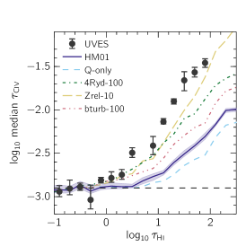
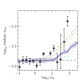
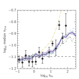
Figure 3: Median recovered pixel optical depths binned by Hi for Civ (left), Siiv (centre) and Ovi (right). Note that the dynamic range shown along the $y$-axis decreases strongly from left to right. The data from eight QSOs have been combined, and the $1\sigma$ error bars are measured by bootstrap resampling the QSOs. The black circles show the data, while the curves denote the results from simulations, where different colours and line styles represent variations in the model and we show the $1\sigma$ error region around the fiducial HM01 model. The flat level $\tau_{\text{min}}$, which is the same for the observations and simulations by construction, is indicated by the dashed horizontal line. The data from the observations is provided in Table 3. The simulation run with the fiducial UVB systematically underpredicts the median Civ and Siiv optical depths. The discrepancy is lessened by invoking a softer UVB (4Ryd-100), higher metallicity (Zrel-10), or unresolved turbulent broadening (bturb-100), although the metal-line optical depths associated with the strongest Hi absorption are still underestimated by $\approx 0.5$ dex. In contrast, the predicted Ovi(Hi) relation (right-hand panel) is insensitive to the UVB models, and in good agreement with the observations.

Table 3: Observational data shown in Fig. 3. The left column indicates the central $\log_{10}\tau_{\rm H\textsc{i}}$ value of each bin, and the next three columns list the $\log_{10}$ median recovered optical depths for the Civ(Hi), Siiv(Hi), and Ovi(Hi) relations, respectively, along with the $1\sigma$ errors. We note that for the bin where $\log_{10}\tau_{\rm H\textsc{i}}=0.70$, the metal optical depths are not defined because there were contributions from fewer that four of our eight quasars.

$\log_{10}\tau_{\rm H\textsc{i}}$	Civ(Hi)	Siiv(Hi)	Ovi(Hi)
$\tau_{\rm min}$	$-2.90$	$-2.85$	$-1.10$
$-0.90$	$-2.94_{-0.06}^{+0.07}$	$-3.01_{-0.09}^{+0.12}$	$-1.12_{-0.03}^{+0.03}$
$-0.70$	$-2.91_{-0.07}^{+0.10}$	$-2.84_{-0.09}^{+0.09}$	$-1.15_{-0.04}^{+0.04}$
$-0.50$	$-2.89_{-0.04}^{+0.04}$	$-2.83_{-0.06}^{+0.08}$	$-1.09_{-0.03}^{+0.04}$
$-0.30$	$-3.04_{-0.10}^{+0.17}$	$-2.87_{-0.07}^{+0.07}$	$-1.14_{-0.04}^{+0.06}$
$-0.10$	$-2.81_{-0.03}^{+0.03}$	$-2.87_{-0.04}^{+0.04}$	$-1.14_{-0.04}^{+0.05}$
$0.10$	$-2.79_{-0.05}^{+0.07}$	$-2.98_{-0.05}^{+0.04}$	$-1.14_{-0.02}^{+0.04}$
$0.30$	$-2.75_{-0.05}^{+0.06}$	$-2.88_{-0.09}^{+0.07}$	$-1.06_{-0.05}^{+0.04}$
$0.50$	$-2.49_{-0.05}^{+0.06}$	$-2.69_{-0.03}^{+0.03}$	$-1.11_{-0.04}^{+0.06}$
$0.70$	…	…	…
$0.90$	$-2.41_{-0.10}^{+0.11}$	$-2.67_{-0.05}^{+0.05}$	$-1.06_{-0.04}^{+0.04}$
$1.10$	$-2.14_{-0.03}^{+0.04}$	$-2.55_{-0.07}^{+0.07}$	$-0.98_{-0.02}^{+0.02}$
$1.30$	$-1.90_{-0.03}^{+0.03}$	$-2.89_{-0.21}^{+0.21}$	$-1.03_{-0.06}^{+0.07}$
$1.50$	$-1.66_{-0.12}^{+0.10}$	$-2.83_{-0.22}^{+0.62}$	$-0.83_{-0.04}^{+0.03}$
$1.70$	$-1.57_{-0.05}^{+0.06}$	$-2.38_{-0.21}^{+0.33}$	$-0.94_{-0.04}^{+0.04}$
$1.90$	$-1.46_{-0.05}^{+0.05}$	$-1.87_{-0.12}^{+0.12}$	$-0.83_{-0.08}^{+0.10}$

3 Results

3.1 $\tau_{Z}$ as a function of $\tau_{\rm HI}$

We begin by examining median metal-line pixel optical depths as a function of Hi pixel optical depth in Fig. 3, where we have plotted Civ(Hi), Siiv(Hi) and Ovi(Hi) from left to right. The grey points with error bars represent the observations, while the curves show results from simulations, with different colours indicating variations in the model. The data from the observations is presented in Table 3.

The relations displayed in Fig. 3 depend on the following quantities in the simulations, using Civ as an illustrative example:

$$\log_{10}\dfrac{\tau_{\rm C\textsc{iv}}}{\tau_{\rm H\textsc{i}}}=\log_{10}\dfrac{(f\lambda)_{\rm C\textsc{iv}}}{(f\lambda)_{\rm H\textsc{i}}}\dfrac{n_{\rm C\textsc{iv}}}{n_{\rm C}}\dfrac{n_{\rm H}}{n_{\rm H\textsc{i}}}+[\text{C}/\text{H}]+(\text{C}/\text{H})_{\odot},$$ (2)

where $f$ is the oscillator strength, $\lambda$ is the rest wavelength, and $n$ is the number density. While the oscillator strength and rest wavelength are fixed empirical quantities, the element abundances are predicted, and the ionization fractions (i.e., the ratio of ionized to total number density) are determined using the particle temperatures and densities in the same manner as was done to compute the cooling rates used in the simulation.

In the following analysis, we will consider the results in two different regimes, separated by $\tau_{\rm H\textsc{i}}\approx 10$. The reasons for this are: (1) For $\tau_{\rm H\textsc{i}}\gtrsim 10$ Hi pixel optical depths will be highly saturated, and even though this is corrected for in our recovery procedure, the final values still suffer from large uncertainties compared to their unsaturated counterparts. (2) If the gas being probed is mainly in photoionization equilibrium, which is a reasonable assumption for Civ and Siiv (Schaye et al., 2003; Aguirre et al., 2004), then Hi is considered a good tracer of the density (Schaye, 2001), even on an individual pixel basis (Aguirre et al., 2002). This means that higher Hi optical depths probe dense regions closer to galaxies, rather than the diffuse IGM.

To touch on this point more quantitatively, we have calculated the optical depth-weighted overdensities for our full sample of mock spectra. Fig. 4 shows the median optical depth-weighted overdensity as a function of Hi for Hi, Civ, Siiv, and Ovi, and we find a strong correlation in every case. We have performed ordinary least-squares fits to the curves using a power-law function:

$$\log_{10}\delta=A\times\log_{10}\tau_{\rm H\textsc{i}}+B,$$ (3)

and give the resulting parameters in Table 4. We note that our aforementioned division of the Hi optical depths into two regimes at $\tau_{\rm H\textsc{i}}\approx 10$ corresponds to an overdensity of $\approx 8$ for the gas responsible for the Hi absorption, but that the overdensity of the metal ions at the same redshifts as the selected Hi pixels is typically a factor of a few lower. We also caution that the quantities presented here are pixel-weighted, and may therefore be biased to high temperatures since higher temperature lines will be more broadened and therefore cover more pixels. This may also bias the densities to lower values, as intergalactic gas with $T\gtrsim 10^{5}$ K tends to correspond to lower densities than that found at lower temperatures. (e.g., Fig. 1 from van de Voort et al., 2011).

The fitted values for Hi can be compared to eq. 8 of Rakic et al. (2012), who used the relations of Schaye (2001) to obtain an expression for overdensity as a function of Hi Ly$\alpha$ line centre optical depth $\tau_{0,{\rm Ly}\alpha}$, under the assumption that the absorbers have sizes of the order of the local Jeans length. Modifying their eq. 8 using the parameters from this work, we obtain:

$$\begin{split}\delta\approx&\,0.74\,\tau_{0,{\rm Ly}\alpha}^{2/3}\ \left(\dfrac{\Gamma_{12}}{0.85\times 10^{12}\text{ s}^{-1}}\right)^{2/3}\left(\dfrac{1+z}{4.36}\right)^{-3}\\ \times&\left(\dfrac{T}{2\times 10^{4}\text{ K}}\right)^{0.17}\left(\dfrac{f_{\rm g}}{0.15}\right)^{-1/3}\left(\dfrac{b}{20\text{ km~{}s${}^{-1}$}}\right)^{2/3}.\end{split}$$ (4)

To determine the redshift $z$, for each QSO we considered the redshift at the centre of the Ly$\alpha$ forest as defined by eq. 1, and took the mean of all of the values. To obtain the photoionization rate $\Gamma_{12}$, we multiplied the photoionization rate from Haardt & Madau (2001) at each of the above redshifts by the scale factor that was used to bring the median recovered Hi optical depth of the mock spectra into agreement with that of the corresponding observed spectrum, and took the mean for all set of mocks. As in Rakic et al. (2012), we chose a temperature typical of a moderately-dense region in IGM (e.g., Schaye et al., 2000a; Lidz et al., 2010; Becker et al., 2011; Rudie et al., 2012b), and assumed that the gas fraction $f_{\rm g}$ corresponds to the universal value of $\Omega_{\rm b}/\Omega_{\rm m}$. Finally, we have taken $b$ to be $20$ km s^-1, which is similar to values measured by Rudie et al. (2012a) for $z\approx 2.5$. Putting eq. 4 into the form of eq. 3, we obtain $A=0.67$ and $B=-0.13$, compared with $A=0.66\pm 0.01$ and $B=0.16\pm 0.01$ measured from our simulations. Hence, the slope $A$ is in excellent agreement with the theoretical scaling relation implied by the model of Schaye (2001). The normalization agrees to within a factor of two, which we consider good agreement given the uncertainties in the fiducial parameter values.

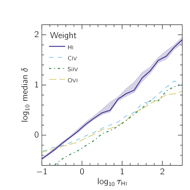
Figure 4: Median optical depth-weighted overdensity as a function of Hi optical depth for the simulated spectra. The different curves indicate the ion used for the weighting. We have indicated the one $1\sigma$ error region around the Hi-weighted overdensity. The parameters from an ordinary least-squares fits of the form $\log_{10}\delta=A\times\log_{10}\tau_{\rm H\textsc{i}}+B$ to each of the relations are given in Table 4. The metal-line absorption typically arises in lower-density gas than the Hi absorption with the same redshift.

Table 4: Results from fitting a power-law $\log_{10}\delta=A\times\log_{10}\tau_{\rm H\textsc{i}}+B$ to the relations in Fig. 4, using ordinary least-squares.

Ion	$A$	$B$
Hi	$0.66\pm 0.01$	$0.16\pm 0.01$
Civ	$0.37\pm 0.02$	$-0.02\pm 0.01$
Siiv	$0.52\pm 0.01$	$-0.24\pm 0.01$
Ovi	$0.36\pm 0.02$	$-0.05\pm 0.01$

With the above in mind, we can interpret the results of Fig. 3. Focusing first on the left-hand panel, we find that at fixed Hi, the observed median Civ optical depths are significantly higher than in the fiducial HM01 model. The discrepancy increases from $\approx 0.1$ dex at $\tau_{\rm H\textsc{i}}=1$ to $\approx 0.5$ dex at $\tau_{\rm H\textsc{i}}=10$ and $\approx 1$ dex at $\tau_{\rm H\textsc{i}}=10^{2}$. This suggests that at a given gas overdensity, there is less Civ in the simulations by $\approx 0.5$ dex ($\approx 1.0$ dex) for $\tau_{\rm H\textsc{i}}\lesssim 10$ ($\tau_{\rm H\textsc{i}}\gtrsim 10$).

Turning to the different UVB models, while the harder Q-only background provides a poorer match to the observations, 4Ryd-100 fares much better. Although this model still falls short of the observed $\tau_{\rm C\textsc{iv}}^{\text{med}}$ by about $\approx 0.5$ dex in the highest $\tau_{\rm H\textsc{i}}$ bin, the softest background is nearly fully consistent with the observations for $\tau_{\rm H\textsc{i}}\lesssim 10$.

From eq. 2, it is apparent that an increase in [C/H] will lead to higher Civ optical depths at fixed Hi. Therefore, we have run SPECWIZARD with the elemental abundances scaled linearly by a factor of ten, denoted as “Zrel-10”. Such a modification can be partially motivated by the fact that we expect some uncertainty in the nucleosynthetic yields, of about a factor of two. We have chosen a factor much larger than this since we find that increasing the metallicities does not scale the median recovered optical depth by the same factor (contrary to what one might expect from eq. 2). This is because many pixels contributing to the median optical depth are noise dominated (particularly at low Hi), and some fraction of these pixels have a true optical depth of zero, so no matter how much the metallicity is increased, the optical depth will never change and exceed the noise.

Although Zrel-10 provides much better agreement between the model and data, even with such an extreme choice of multiplicative factor it cannot fully account for the discrepancy between the simulations and data. This suggests that in the simulation too many Hi clouds have negligible metallicity. To check this, we have calculated the mass and volume filling factors of the metals using eq. 1 from Booth et al. (2012) The authors determined that $>10$% of the volume and $>50$% of the mass need to be enriched to metallicities $Z>10^{-3}$ Z_⊙ to achieve agreement with observations of Civ in the low-density IGM at $z\approx 3$. For the fiducial L100N1504 box at $z=3.5$ and $Z>0$ we find volume and mass filling factors of 42% and 68%, but for $Z>10^{-3}$ Z_⊙ these are reduced to 10% and 19%, respectively. This suggests that while the fractions of the volume and mass with non-zero metallicity may be sufficiently high, the metallicities in the photo-ionised IGM are typically far too low.

Next, we describe another modification to our fiducial model denoted as “bturb-100”, for which we have considered an unresolved turbulent broadening term in addition to the usual thermal broadening. Specifically, we add $b_{\rm turb}=100$ km s^-1 in quadrature to the already included thermal broadening $b_{\rm therm}(T,m)$ which is calculated for every ion at each spectral pixel, and depends on the local temperature $T$ and inversely on atomic mass $m$. Because of this inverse dependence on atomic mass, metal ions will be much more strongly affected by the inclusion of turbulent broadening than Hi. Indeed, we find that bturb-100 provides a somewhat better match to the observed Civ(Hi) relation. However, we note that our chosen broadening value $100$ km s^-1 should be considered a very conservative upper limit, as individual Civ and Siiv components are not usually detected with such large $b$-parameters.

In the centre panel of Fig. 3, we show Siiv(Hi), and find results that are similar to those for Civ(Hi). For $\tau_{\rm H\textsc{i}}\gtrsim 10$ the Siiv optical depths are underestimated by the fiducial HM01 model by a factor ranging from $\approx 0.2$ dex at $\tau_{\rm H\textsc{i}}=10$ up to $\approx 0.8$ dex at $\tau_{\rm H\textsc{i}}=10^{2}$. Invoking 4Ryd-100 leads to near agreement for all but the highest Hi optical depth, while Zrel-10 and bturb-100 also fare markedly better than the fiducial model.

We now consider the Ovi(Hi) relation in the right-hand panel of Fig. 3. While Civ and Siiv are expected to mainly probe cool photoionized gas ($T\sim 10^{4}$ K), Ovi reaches its peak ionization fraction of 0.2 at $T=3\times 10^{5}$ K, which is close to the temperatures expected of shocks associated with accretion events or winds. Simulations predict that Ovi around galaxies is primarily collisionally ionized (e.g. Tepper-García et al., 2011; Stinson et al., 2012; Ford et al., 2013; Shen et al., 2013). Applying ionization modelling to observations also provides evidence that Ovi near moderate to strong Hi preferentially probes this hot gas phase (e.g, Simcoe et al., 2004; Aguirre et al., 2008; Danforth & Shull, 2008; Savage et al., 2014; Turner et al., 2015).

Indeed, the results from the right-hand panel of Fig. 3 differ considerably from the previous two relations. Firstly, the simulation realized with the fiducial model is almost fully consistent with the observations, with any discrepant points offset by a maximum of 0.2 dex (note the smaller dynamic range of the y-axis compared to the previous panels). While the alternate UVBs (Q-only and 4Ryd-100) have slightly lower $\tau_{\rm O\textsc{vi}}$ than the fiducial case, overall we do not find significant differences between these models. This suggests that in EAGLE the Ovi(Hi) relation may be probing a primarily collisionally ionized gas phase, for which variations in the ionization background do not have a significant impact on the results. Furthermore, the fact that the median Ovi optical depth appears to be largely insensitive to the addition of turbulent broadening could indicate that Ovi is already significantly thermally broadened. We note that if the pixel optical depths do not originate predominantly from photoionized gas, then $\tau_{\rm H\textsc{i}}$ can no longer be used as a measure of the density.

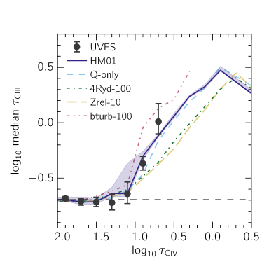
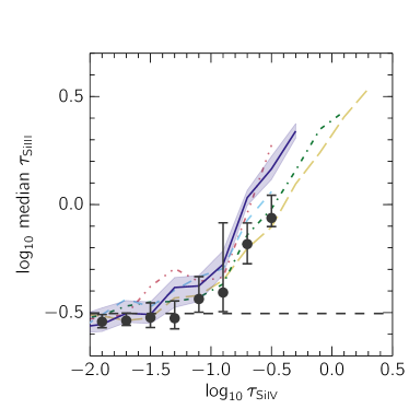
Figure 5: The same as Fig. 3, but showing Ciii(Civ) and Siiii(Siiv), and with the data from observations presented in Table 5. Unlike for relations binned by Hi, different ionization states of the same element are not sensitive to the metallicity of the gas. We find that for Ciii(Civ), the simulations and data are in good agreement for the fiducial ionizing background, and the observations particularly disfavour 4Ryd-100 and Zrel-10. The Siiii(Siiv) relation is somewhat less constraining, and while the median Siiii optical depths from HM01 model are slightly above the observed values, the discrepancy is no more than 0.1 dex and only seen in the highest Siiv bins. This indicates that the temperature and density of the gas probed by pixels with detected Civ and and Siiv is well captured by the simulations, without needing to invoke modifications to the model.

Table 5: Observational data from Figs. 5 and 6. The format is the same as Table 3, but here we present relations binned by either Civ or Siiv optical depths. The left column indicates the central value of the Civ or Siiv bin, and the subsequent columns list the median recovered optical depths for the relation denoted in the top row.

$\log_{10}\tau_{\rm bin}$	Ciii(Civ)	Siiii(Siiv)	Siiv(Civ)	Ovi(Civ)	Ovi(Siiv)
$\tau_{\rm min}$	$-0.70$	$-0.50$	$-2.78$	$-1.06$	$-1.10$
$-1.90$	$-0.68_{-0.02}^{+0.02}$	$-0.54_{-0.03}^{+0.03}$	$-2.84_{-0.03}^{+0.03}$	$-1.17_{-0.05}^{+0.08}$	$-1.12_{-0.04}^{+0.03}$
$-1.70$	$-0.71_{-0.03}^{+0.03}$	$-0.54_{-0.02}^{+0.04}$	$-2.82_{-0.06}^{+0.05}$	$-1.07_{-0.03}^{+0.03}$	$-1.10_{-0.02}^{+0.03}$
$-1.50$	$-0.72_{-0.04}^{+0.04}$	$-0.52_{-0.05}^{+0.07}$	$-2.64_{-0.04}^{+0.05}$	$-1.02_{-0.02}^{+0.02}$	$-1.08_{-0.04}^{+0.04}$
$-1.30$	$-0.72_{-0.07}^{+0.08}$	$-0.53_{-0.05}^{+0.08}$	$-2.45_{-0.05}^{+0.05}$	$-1.05_{-0.04}^{+0.04}$	$-0.99_{-0.05}^{+0.03}$
$-1.10$	$-0.64_{-0.09}^{+0.11}$	$-0.44_{-0.06}^{+0.10}$	$-2.21_{-0.05}^{+0.05}$	$-0.95_{-0.02}^{+0.02}$	$-0.99_{-0.04}^{+0.05}$
$-0.90$	$-0.37_{-0.06}^{+0.06}$	$-0.41_{-0.09}^{+0.32}$	$-1.98_{-0.05}^{+0.07}$	$-1.00_{-0.09}^{+0.15}$	$-0.86_{-0.03}^{+0.04}$
$-0.70$	$0.01_{-0.11}^{+0.16}$	$-0.18_{-0.09}^{+0.10}$	$-1.57_{-0.10}^{+0.18}$	$-0.66_{-0.07}^{+0.08}$	$-0.81_{-0.09}^{+0.29}$
$-0.50$	…	$-0.06_{-0.04}^{+0.10}$	$-1.07_{-0.20}^{+0.19}$	$-0.43_{-0.04}^{+0.03}$	$-0.90_{-0.15}^{+0.54}$
$-0.30$	…	…	$-1.87_{-0.17}^{+0.36}$	$-0.82_{-0.09}^{+0.31}$	…
$-0.10$	…	…	$-0.82_{-0.01}^{+0.34}$	$-0.40_{-0.00}^{+0.04}$	…

3.2 $\tau_{Z}$ as a function of $\tau_{\rm CIV}$ and $\tau_{\rm SiIV}$

While metal ions as a function of $\tau_{\rm H\textsc{i}}$ can probe the metallicity-density relation, examining different ionization states of a single element can provide insight into the physical properties of the gas, because the ionization fractions that set the relative optical depths will only depend on the temperature, the density, and the UV radiation field (and not on the metallicity, but see below). These optical depth ratios have previously been used to establish that the gas probed by Civ and Siiv is consistent with being in photoionization equilibrium (Schaye et al., 2003; Aguirre et al., 2004).

Fig. 5 examines Ciii(Civ) and Siiii(Siiv), and the observational data is provided in Table 5. Looking first at Ciii(Civ), we find that HM01 is consistent with all of the Civ bins. Both the bturb-100 and Q-only models also agree with the data, which is notable in particular for Q-only as it is the most disfavoured by the Civ(Hi) relation. Finally, we find that the 4Ryd-100 and Zrel-10 models fare particularly poorly in this relation, and produce median Ciii optical depths lower than the observations by up to 0.4 dex. In particular, for Zrel-10 such a discrepancy may seem surprising, since changing the carbon abundance should not affect the amount of one ionization state against another. However, the reason this occurs is because Civ increases more than Ciii, which is due to the fact that many more Ciii pixels are contaminated and hence do not change.

Next, we find the Siiii(Siiv) relation to be somewhat less constraining. While the fiducial HM01 model demonstrates one of the largest discrepancies with the data, the difference is not more than $\approx 0.1$ dex when the errors are considered, and is only seen in the highest Siiv bins. Thus, we find good agreement between the data and the fiducial model for both relations, which suggests that the temperature and density of the gas probed by Civ and Siiv pixels is consistent between the observations and simulations.

We note that the above result is not in tension with the results shown in Fig. 3. Namely, while Fig. 3 indicates that there is a lack of Civ and Siiv in the simulations, Fig. 5 demonstrates that the Siiv and Civ that we do find in the mock spectra, regardless of the amount, likely resides in gas with similar temperature and density as in the observations.

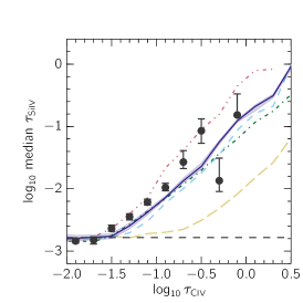
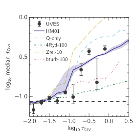
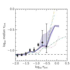
Figure 6: The same as Fig. 3, except showing Siiv(Civ), Ovi(Civ) and Ovi(Siiv) from left to right, which probe relative abundances. The data from the observations is given in Table 5. In the left-hand panel, we find that $\tau_{\rm Si\textsc{iv}}^{\text{med}}$ is underestimated by all models except bturb-100, and is insensitive to the choice of UVB. Next, for Ovi(Civ) and Ovi(Siiv) we observe a stronger sensitivity to different ionizing background models and turbulent broadening compared to Ovi(Hi). For these relations, we observe a better match between the fiducial and hardest UVB models (HM01 and Q-only), in tension with the results from Civ(Hi) and Siiv(Hi) relations, where we find a strong preference for the softer ionization backgrounds (see Fig. 3).

In Fig. 6 we examine relations between different metal ions, which trace relative abundances and physical conditions. The data for this figure is provided in Table 5. For example, Si/C, which can be estimated using the Siiv(Civ) relation, has been found to be greater than solar by a factor of a few in the IGM (e.g., Songaila, 2001; Boksenberg et al., 2003; Aguirre et al., 2004).

In the left-hand panel of Fig. 6, we plot the median Siiv optical depth against Civ. While the results are not very sensitive to the choice of ionizing background, all models except bturb-100 present a paucity of Siiv with respect to the observations. In particular, the median Siiv  optical depth from the Zrel-10 model shows an offset of $\leq-1$ dex from the observations at fixed Civ. Again, this is due to the fact that for Siiv, many more pixels that contribute to the median optical depth are noise dominated compared to Civ, and therefore do not change when the metallicity is increased. For the remaining models that use the metallicities directly from the simulations, this may indicate that at $z\sim 3.5$ the simulations have lower [Si/C] than observed. Additionally, as evidenced by the bturb-100 model, turbulent broadening, which has the strongest influence on the heavy silicon atoms, could perhaps be invoked to alleviate this discrepancy.

We briefly draw attention to the bin centred at $\log_{10}\tau_{\rm C\textsc{iv}}=-0.3$, where the observed median Siiv optical depth deviates starkly from the rest of the points. The same behaviour is also seen in the central panel of Fig. 6, in which we examine Ovi(Civ). To find the origin of this inconsistency, we turn to the relations of individual QSOs, in Figs. 15 and 16. In the case of Q1317$-$507 (the upper right-hand panel of both figures), the median Siiv and Ovi optical depths are unusually low in this Civ bin, while having relatively small error bars (the median optical depths of different QSOs are combined in linear space). We conclude that these points from Q1317$-$507, likely the result of small number statistics, are responsible for the anomaly in the Siiv(Hi) and Civ(Hi) relations.

The centre panel of Fig. 6 shows $\tau_{\rm O\textsc{vi}}^{\text{med}}$ binned by $\tau_{\rm C\textsc{iv}}$. In contrast to the Ovi(Hi) relation (Fig. 3, right-hand panel), it is apparent that the median Ovi(Civ) optical depth depends strongly on the choice of UVB, and is sensitive to both an increase in the elemental abundances and the addition of turbulent broadening. This is consistent with the picture that Civ primarily traces photoionized gas, which will depend on the choice ionizing background, and will not be as thermally broadened as hot, collisionally ionized gas. We find that the fiducial HM01 model is in broad agreement with the data for this relation, even when including the bin centred at $\log_{10}\tau_{\rm C\textsc{iv}}=-0.3$, while softer UVB models predict too weak Ovi at high $\tau_{\rm C\textsc{iv}}$. If the Ovi that is coincident with strong Civ were photoionized, then this would be a useful constraint. However, unlike Civ, Ovi may well be collisionally ionized.

Finally, in the right-hand panel of Fig. 6 we show Ovi(Siiv). Except for $\log_{10}\tau_{\rm Si\textsc{iv}}\gtrsim-0.5$, we observe a much weaker dependence on the models than for Ovi(Civ), but we still find that HM01, in addition to Q-only and Zrel-10, provides the best match to the data.

3.3 Physical conditions of the gas

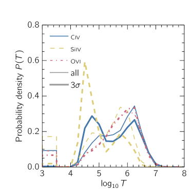
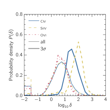
Figure 7: PDFs of the optical depth-weighted temperature (left) and overdensity (right), where the line colour and style indicates the ion used for weighting. The narrower lines represent the full sample of pixels that have $\tau_{\rm H\textsc{i}}>10$, and the thicker line PDFs were calculated using this same sample but with the additional constraint that the metal-line optical depth had to be $3\sigma$ above the flat level, $\tau_{\text{min}}$. This second cut is used to isolate pixels that have a significant optical depth detection. The PDF offset to the left of the main distribution denotes pixels that have zero temperature and density. By definition these pixels have zero metallicity, but a detected optical depth due to noise or contamination. We find that Civ and Siiv probe a bimodal range of temperatures, while pixels with higher Ovi optical depths primarily arise in hot gas.

In this section, we examine the temperatures and densities of the gas probed by our optical depth relations. In Fig. 7, we have plotted the probability density functions (PDFs) of the optical depth-weighted temperatures (left) and densities (right) from our simulations. In particular, we are interested in the physical properties of the regions from which we detect signal in Fig. 3. We therefore only consider pixels with $\tau_{\rm H\textsc{i}}>10$, to focus on areas where we find the largest discrepancy between observations and mock spectra in this figure.

The resulting PDFs are shown as the solid lines in Fig. 7, and demonstrate high temperatures, which may be surprising for Siiv and Civ, which we expected to be at least somewhat photoionized. However, these PDFs are biased to high temperatures because higher temperature gas is more broadened. For a single absorption line at high temperature, the optical depths will hence be spread over more pixels, and the individual pixel optical depth values will be lower than for a lower temperature region. This effect is further amplified by the fact that the pixel optical depth-weighted temperatures are averages over the linear (rather than log) temperatures of different gas elements. This means that gas elements with relatively low ion fractions but high temperatures can affect the weighted means. Furthermore, at low density the ionization fraction peaks with temperature become much less prominent if photoionization is included (see e.g. Fig. 1 of Rahmati et al. 2016).

In an effort to combat this bias, we then make an additional cut, where we only take pixels that have a metal-line optical depths $3\sigma$ above the corresponding flat level $\tau_{\text{min}}$. The result of making this additional cut is shown as the dashed line in Fig. 7. First, we find that the temperature and density PDF for Ovi is unchanged, which indicates that most of the signal for Ovi truly comes from gas with higher temperatures (although the distribution is still quite broad, consistent with Oppenheimer et al. 2016). On the other hand, for Civ- and Siiv-weighted quantities this cut reveals a bi-modal temperature distribution, where many of the pixels probe cooler, $\approx 10^{4.5}$ K gas. Likewise, the Ovi-weighted overdensities are not affected by the $3\sigma$ cut, while for Civ and Civ the overdensity PDFs are still unimodal but have shifted to higher values. Overall, this figure indicates that while most of the signal for Ovi(Hi) comes from hot ($T\gtrsim 10^{5}$) gas with $\delta\sim 1$–$10$, a substantial portion of the pixels that lead to the Civ(Hi) and Siiv(Hi) relations arise from cooler, likely photoionized gas at $\sim 10^{4.5}$ K with overdensities $\gtrsim 10$.

4 Discussion

In the previous section, we compared observations of pixel optical depth relations to the EAGLE simulations. We considered a fiducial QSO+galaxy HM01 UVB (Haardt & Madau, 2001), as well a harder QSO-only model, and a softer UVB with reduced intensity above 4 Ryd by a factor of 100. For Ovi(Hi), we found an insensitivity to the ionizing background model, and saw good agreement between the simulations and the data. However, the observed median optical depths from the Civ(Hi) and Siiv(Hi) relations were measured to be systematically higher than those derived from the simulations using the fiducial UVB. The discrepancy is smaller than $\approx 0.5$ dex below $\tau_{\rm H\textsc{i}}=10$ but can reach up to 1 dex for Hi bins above this threshold. For Siiv(Hi), invoking 4Ryd-100 fully alleviates the tension, while for Civ(Hi) we find this model still falls short of the data, but only for $\tau_{\rm H\textsc{i}}\gtrsim 10$. We also find that increasing the metallicity by a factor of ten (Zrel-10) and manually broadening the absorption lines to take unresolved turbulence into consideration (bturb-100) do not fully resolve the discrepancy. In this section, we discuss in more detail possible reasons for the observed mismatch.

Can the discrepancies between the observations and simulations be attributed to differences in the UVB? We have indeed found better agreement with the observed Civ(Hi) and Siiv(Hi) relations using our softest UVB intended to explore the effects of delayed Heii reionization, 4Ryd-100. The reduced intensity above 4 Ryd disfavours ionization to higher states, increasing the abundances of Siiv and Civ. While Haardt & Madau (2001) models take Heii reionization into account and predict that the Heiii fraction already reaches 50% at $z\approx 6$, recent studies suggest that the reionization process is patchy, with Heii optical depths still high above $z\gtrsim 3$ (e.g., Shull et al., 2010; Worseck et al., 2011). Thus, the work presented here probes the epoch where the observed gas may be subject to a strongly fluctuating UVB above 4 Ryd. The much better match of the 4Ryd-100 UVB suggests that Heii reionization could be complete too early in the simulations. Turning to other optical depth relations, we find that Ciii(Civ) and Siiii(Siiv) do not strongly rule out the 4Ryd-100 model. While these soft UVBs are inconsistent with Ovi(Civ), the problem occurs only for $\log_{10}\tau_{\rm C\textsc{iv}}\gtrsim-0.7$, which is higher than relevant for Fig. 3.

An alternative effect could be the presence of ionization due to stellar light from nearby galaxies, which is thought to be important for absorbers as rare as Lyman limit systems (Schaye, 2006; Rahmati et al., 2013b). The strength of the ionizing radiation emitted by galaxies drops sharply above 4 Ryd, but could strongly ionize Hi, lowering the typical optical depths. If Hi optical depths are lower, than at a fixed Hi the metal-line optical depths will be higher. This could explain the larger discrepancy seen at $\tau_{\rm H\textsc{i}}\gtrsim 10$, where the pixel optical depths are probing denser gas at small galactocentric distances compared to lower Hi optical depths. However, since it is difficult to estimate the shape and normalization of this ionizing radiation (and it likely should not be applied uniformly), we leave testing of this explanation to a future work.

We have also considered the effects of turbulent broadening. It is certainly true that our fiducial model misses the unresolved turbulence from the dense particles on the imposed EoS (where by fixing the temperatures to $10^{4}$ K we neglect a possibly significant fraction of the energy), and possible that turbulence in other regions is also underestimated. Indeed, we find that by artificially broadening metal ion absorption lines, we are able to bring the Civ(Hi) and Siiv(Hi) relations into slightly better agreement with observations. Furthermore, the inclusion of $b_{\rm turb}$ may help alleviate the tension between the observed and simulated Siiv(Civ). However, we stress that our implementation provides a very conservative upper limit on this effect, because (a) we use a very high $b$-parameter (100 km s^-1) and (b) we apply the turbulent term to all metal-line absorption pixels, not just those in very high density regions or with contributions from particles on the EoS.

Another possibility for the observed discrepancy is that the metallicity of the intergalactic gas in the simulations is too low. Using our Zrel-10 model, we have examined the effect of increasing the elemental abundances linearly by a factor of ten. While such a change in metallicity is larger than the expected metal yield uncertainties, it is still unable to increase the simulated median Civ and Siiv at fixed Hi enough to agree with observations. Furthermore, increasing the metallicities of both carbon and silicon by equal amounts leads to disagreement between the simulated and observed Siiv(Civ) relation, since the optical depths do not scale directly with metallicity in the same way due to differences in contamination and noise.

A related issue may be that the that the metals are not transported far enough into the IGM. An insufficient volume filling fraction of enriched gas could arise if the simulations do not resolve the low-mass galaxies thought to be important for metal pollution (e.g., Wiersma et al., 2010; Booth et al., 2012). In Appendix B, we examined results from simulations with higher resolution than our fiducial model (the Ref- and Recal-L025N0752 runs). These simulations can resolve galaxies (containing at least 100 star particles) with $M_{\star}=2.3\times 10^{7}$ M_⊙, almost an order of magnitude below that of our fiducial model, where a 100 star particle galaxy would have stellar mass of $1.8\times 10^{8}$ M_⊙. Indeed, we find that relations involving Civ are not fully converged at our fiducial resolution, and invoking the highest-resolution model for Civ(Hi) results in an increase in $\tau_{\rm C\textsc{iv}}^{\text{med}}$ of up to $\approx 0.3$ dex in the highest Hi bins.

To investigate the reason for the resolution dependence, we have imposed the same metallicity-density relation on both Ref-L025N0752 and Ref-L025N0376, finding no significant differences in the optical depth relations. This implies that the better agreement with observations with increasing resolution is not caused by changes in the density-temperature structure of the gas. We have also calculated the average metallicites for the various resolutions in the 25 cMpc volume, and find that the differences are small (varying at most by a factor of 1.2). Furthermore, we find that the mean gas-particle metallicity is lowest in Recal-L025N0752, and highest in Ref-L025N0188. Therefore, the increase in Civ(Hi) with resolution is not due to an increase in the total amount of metals, but rather to an increase of the metallicity of the IGM. This suggests that winds ejected from galaxies with stellar masses below $\approx 1.8\times 10^{8}$ M_⊙ are likely important for IGM pollution. While a simulation with higher resolution may bring the observations and simulations closer to agreement, the effect does not appear to be strong enough to fully explain the differences seen in the Civ(Hi) relation, and furthermore, the Siiv(Hi) relation shows almost no change when the resolution is increased. Therefore, we believe that additional factors may be at play.

An important piece of information to consider is the much better agreement between the observed and simulated Ovi(Hi) relations. The insensitivity of $\tau_{\rm O\textsc{vi}}^{\text{med}}$ (when binned by Hi) to the different UVB models suggests that the gas is primarily collisionally ionized, and hence that Ovi(Hi) is probing a hotter ($T\gtrsim 10^{5}$ K) gas phase than Civ(Hi) and Siiv(Hi), as also found for $\tau_{\rm H\textsc{i}}>10$ by Aguirre et al. (2008). From this, we can conclude that for hot gas, the physical properties probed by the pixel optical depth relations are consistent with observations of the IGM at $z\sim 3.5$. The lack of Civ and Siiv, on the other hand, may not be due to a too low metallicity or volume filling fraction, but rather to an incorrect gas phase. If too much of the enriched gas is excessively hot, then too much carbon and silicon will be ionized to states above Civ and Siiv, reducing the number of pixels with detectable Civ and Siiv absorption.

Aguirre et al. (2005) found an even more severe underestimation of simulated median Civ optical depths, with the tension also being alleviated by invoking a softer UVB. In contrast to EAGLE, the simulations in Aguirre et al. (2005) did not include metal-line cooling, and that study found that most of the metals resided in an unrealistically-hot gas phase ($10^{5}\lesssim T\lesssim 10^{7}$ K). The authors speculated that the simulations could be brought into agreement with the observations by implementing metal-line cooling, but here we have shown that this is not the case. However, the inclusion of metal-line cooling may have aided in resolving other issues. While we find good agreement between our observations and simulations of the Ciii(Civ) relation, Aguirre et al. (2005) measured a far too low $\tau_{\rm C\textsc{iii}}^{\text{med}}$, indicating a much stronger mismatch in the temperature and/or density of the gas in their simulations.

It may be that the temperature of the metal-enriched gas in our simulations is sensitive to the details of the stellar feedback. It is implemented thermally, using a stochastic prescription in which the temperature of the directly heated gas is guaranteed to initially exceed $10^{7.5}$ K (Dalla Vecchia & Schaye, 2012). The probability of heating events was calibrated to observations of galaxy stellar masses and disc sizes at $z\approx 0$, but observations of the CGM were not considered. In Fig. 7 we established that much of the signal for the Civ(Hi) and Siiv(Hi) relations comes from pixels with temperatures $T~{}\sim 10^{4.5}$ K and overdensities $\delta\gtrsim 10$. This suggests that at $z\sim 3.5$, the outflows driven by stellar feedback may not entrain enough cool ($T\sim 10^{4}$ K) gas. While Furlong et al. (2015b) found that galaxy star formation rate densities and stellar masses are in good agreement with observations for $z\sim 3$–$4$, the work presented here suggests that other indicators may be needed to test fully the feedback implementation at these redshifts.

5 Conclusion

In this work we used pixel optical depth relations to study the $z\sim 3.5$ IGM, using new, very high-quality data for a sample of eight $\langle z_{\text{QSO}}\rangle=3.75$ QSOs, and compared our results with the EAGLE hydrodynamical simulations of galaxy formation. The QSOs were observed with VLT/UVES, and their spectra all have similar S/N and coverage. We employed the pixel optical depth technique to obtain Hi and metal-line absorption partially corrected for the effects of noise, contamination, and saturation. A public version of the code used can be found at https://github.com/turnerm/podpy. The resulting pixel optical depth relations were compared to those derived from mock spectra generated from the EAGLE simulations. The mock spectra were synthesized to have a resolution, pixel size, S/N and wavelength coverage closely matched to the observations. We have considered a fiducial QSO+galaxy UVB (Haardt & Madau, 2001), as well as a harder QSO-only model and a model for which the intensity above 4 Ryd was reduced by a factor of 100. The fiducial EAGLE model was run in a cosmologically representative box size (100 cMpc) at a relatively high resolution ($2\times 1504^{3}$ particles), and the feedback from star formation and AGN was calibrated to reproduce the $z\approx 0$ galaxy stellar mass function, galaxy-black hole mass relation, and galaxy disc sizes. Our conclusions are listed below.

• We detect strong correlations for the observed median Civ(Hi), Siiv(Hi), Ovi(Hi) pixel optical depth relations (Fig. 3), as well as for Ciii(Civ) and Siiii(Siiv) (Fig. 5), and for Siiv(Civ), Ovi(Civ) and Ovi(Siiv) (Fig. 6).

• We find that for the Civ(Hi) and Siiv(Hi) relations, the observed metal-line optical depths are higher than in the simulations run with the fiducial HM01 UVB. For Civ(Hi), we find a discrepancy of up to $\approx 0.1$ dex at $\tau_{\rm H\textsc{i}}=1$, $\approx 0.5$ dex at $\tau_{\rm H\textsc{i}}=10$, and $\approx 1$ dex at $\tau_{\rm H\textsc{i}}=10^{2}$, where we believe we are probing gas at high densities and small galactocentric distances. For Siiv(Hi), while the agreement is slightly better, the behaviour is qualitatively similar to that of Civ(Hi), and we find that the observed optical depths are higher than seen in the simulations by up to $\approx 0.2$ dex at $\tau_{\rm H\textsc{i}}=10$ and by up to $\approx 0.8$ dex at $\tau_{\rm H\textsc{i}}=10^{2}$. In contrast, Ovi(Hi), which probes a hotter gas phase, exhibits much better agreement (i.e. differences smaller than 0.2 dex) with the data for all Hi bins (Fig. 3).

• We consider UVBs that differ from the fiducial HM01 model, including a harder quasar-only background (Q-only) and softer backgrounds with 100 times reduced intensity above 4 Ryd (4Ryd-100). The softer models, which may be more realistic than our fiducial background if Heii is still partially ionized at $z\sim 3.5$, are a better match to the Civ(Hi) and Siiv(Hi) relations, and can nearly reproduce the observations for $\tau_{\rm H\textsc{i}}\lesssim 10$. The results of the Ovi(Hi) relation are however insensitive to the change in UVB, which suggests that Ovi is tracing predominantly collisionally ionized gas (Fig. 3).

• We also test a model where the elemental abundances are increased linearly by a factor of 10 (Zrel-10), and a model where the absorption is broadened by 100 km s^-1  (bturb-100). These variations are meant to explore the effects of uncertainties in the metal yields and of unresolved turbulence, respectively. In both cases we find that the simulated Civ(Hi) and Siiv(Hi) relations are in better (but not full) agreement with the observations, and stress that in we have chosen very aggressive values for our models such that we would expect the actual effects from uncertainties to be smaller (Fig. 3).

• Examining relations that investigate different ionization states of the same element, Ciii(Civ) and Siiii(Siiv), we find good agreement between the observations and simulations for the fiducial HM01 model as well as Q-only and bturb-100. However, the observations disfavour the 4Ryd-100 and Zrel-10 models (Fig. 5).

• Most models demonstrate a mild paucity of $\tau_{\rm Si\textsc{iv}}$ in the Siiv(Civ) relation, which suggests the simulations may have a slightly too low [Si/C]. The two exceptions are bturb-100, which is in good agreement with the observations, and Zrel-100, which demonstrates substantially too little Siiv at fixed Civ (left-hand panel of Fig. 6).

• Unlike Ovi(Hi), the Ovi(Civ) and Ovi(Siiv) relations exhibit sensitivity to the UVB for $\tau_{\rm C\textsc{iv}}\gg 10^{-1}$ and $\tau_{\rm Si\textsc{iv}}\gtrsim 1$, and we find that Ovi(Civ) is best described by the hardest models (the fiducial HM01 and Q-only). The dependence on the ionizing background suggests that strong Civ and Siiv typically probe a cooler ($T\sim 10^{4}$ K), photoionized gas phase compared to the gas traced by Ovi(Hi) (centre and right-hand panels of Fig. 6).

• We use the simulations to examine the PDFs of the optical depth-weighted temperatures and densities of the pixels responsible for the high optical depth values in Fig. 3. We find that while Civ, Siiv and Ovi all have a component probing hot $T\gtrsim 10^{5}$ gas, the Civ and Siiv optical depths mainly arise from a phase of cooler ($\sim 10^{4.5}$ K) gas with $\delta\gtrsim 10$ (Fig. 7).

• We discuss possible reasons why Civ and Siiv optical depths with associated Hi are underestimated by the fiducial simulations, and we consider that perhaps a combination of a number of explanations are responsible:

  1. Ionization by local sources, which the simulations do not account for, may play an important role. Since the strength of the radiation emitted by stars typically falls sharply above 4 Ryd, this would ionize Hi while having a much weaker effect on the metals, which would increase the median metal-line absorption for a fixed Hi optical depth (see e.g. § 4.2 and Fig. 9 in Turner et al. 2015). This explanation is particularly viable for $\tau_{\rm H\textsc{i}}\gtrsim 10$, where we may be probing small galactocentric distances.

  2. The completion of Heii reionization in the HM01 simulations may occur too early, or it may be too uniform, since the observations indicate that it could be quite patchy around $z\sim 3.5$ (e.g., Shull et al., 2010; Worseck et al., 2011). This explanation is supported by the better agreement between the 4Ryd-100 model and the Civ(Hi) and Siiv(Hi) observations. However, even the 4Ryd-100 model cannot fully explain the Civ(Hi) observations for $\tau_{\rm H\textsc{i}}\gtrsim 10$.

  3. The magnitude of line-broadening, particularly in dense star-forming regions, could be underestimated due to unresolved turbulence in the simulations. While artificially adding a large turbulent broadening term slightly increases the median Civ and Siiv optical depths when binned by Hi, the effect is not large enough to explain the observed discrepancy.

  4. The metallicities may not be high enough in the simulations, due to uncertainties in the yields. However, even scaling the metallicities by a factor of 10 is not enough to achieve agreement in the case of Civ(Hi). Furthermore, this scaling creates tension in the Siiv(Civ) relation, due to the fact that the median recovered optical

  5. The simulations may not resolve the low-mass galaxies required to pollute the diffuse IGM. We find that the highest-resolution simulations, Ref- and Recal-L025N0752, exhibit superior agreement with the observed Civ(Hi) relation by $\approx 0.3$ dex at $\tau_{\rm H\textsc{i}}\approx 10^{2}$. While resolution likely plays a role, the magnitude of the effect does not appear large enough to explain fully the discrepancy, particularly for the Siiv(Hi) relation, which we find to be almost insensitive to the resolution increase.

  6. The stellar feedback in the simulations may be driving outflows that contain insufficient cool gas ($T\sim 10^{4}$ K). The relatively good agreement between the observed and simulated Ovi(Hi) relation, which probably traces collisionally ionized gas, indicates that the simulations correctly capture this hotter gas phase ($T\gtrsim 10^{5}$ K), and that it contains enough metals. However, if too much of the enriched gas is hot with respect to the observations, then more Civ and Siiv will be ionized to higher energy levels, leading to a paucity of pixels with detected $\tau_{\rm C\textsc{iv}}$ and $\tau_{\rm Si\textsc{iv}}$.

Overall, while the EAGLE simulations qualitatively reproduce all of the pixel optical depth correlations seen in our sample of QSOs, the mock spectra are found to have less Civ and Siiv at a given density than in the observations. This suggests that the simulations are still missing one or more important components, which we have tested in this work: a more rigorous treatment of Heii reionization to create a softer UVB, the resolution required to model turbulence that contribute to line broadening, and/or higher metallicities and volume filling factors. However, we do not find that any of the above models are individually able to match the observations. While it is possible that the addition of enhanced photoioniziation of Hi by sources close to the absorbers may play an important role, the fact that the simulations agree with the observed Ovi(Hi) relation indicates that the fiducial model is at least able to capture the hot gas phase correctly. Therefore, we believe that it is likely that the outflows created by energetic stellar feedback in the simulations entrain insufficient cool gas.

Appendix A Transitions

In tables 6 and 7, we show the rest wavelengths and oscillator strengths of all Hi and metal-line transitions, respectively, used to create our mock spectra. The data are taken from Morton (2003).

Table 6: Information about the Hi transitions used to create the mock spectra, taken from Morton (2003). From left to right the columns denote the transition, rest wavelength $\lambda$ in angstroms, and oscillator strength $f$.

Transition	$\lambda$ (Å)	$\log_{10}f$
Hi	1215.7	-0.38
	1025.7	-1.10
	972.5	-1.54
	949.7	-1.86
	937.8	-2.11
	930.7	-2.32
	926.2	-2.50
	923.2	-2.65
	921.0	-2.79
	919.4	-2.92
	918.1	-3.04
	917.2	-3.14
	916.4	-3.24
	915.8	-3.33
	915.3	-3.41
	914.9	-3.49
	914.6	-3.57
	914.3	-3.64
	914.0	-3.71
	913.8	-3.77
	913.6	-3.83
	913.5	-3.89
	913.3	-3.94
	913.2	-4.00
	913.1	-4.05
	913.0	-4.10
	912.9	-4.15
	912.8	-4.19
	912.8	-4.24
	912.7	-4.28
	912.6	-4.32

Table 7: The same as table 6, but for metal-line transitions.

Transition	$\lambda$ (Å)	$\log_{10}f$
Cii	1334.5	-0.89
	1036.3	-0.91
Ciii	977.0	-0.12
Civ	1548.2	-0.72
	1550.8	-1.02
Feii	1144.9	-1.08
	1608.5	-1.24
	1063.2	-1.26
	1096.9	-1.49
	1260.5	-1.62
	1122.0	-1.54
	1081.9	-1.90
	1143.2	-1.72
	1125.4	-1.81
Nv	1238.8	-0.80
	1242.8	-1.11
Ovi	1031.9	-0.88
	1037.6	-1.18
Siii	1260.4	0.00
	1193.3	-0.30
	1190.4	-0.60
	989.9	-0.88
	1526.7	-0.94
	1304.4	-1.03
	1020.7	-1.55
Siiii	1206.5	0.22
Siiv	1393.8	-0.29
	1402.8	-0.59

Appendix B Resolution tests

In this appendix, we test the numerical convergence of the EAGLE simulations. We first examine the effects of varying the simulation box size. In Fig. 8, where we show optical depth relations derived from the fiducial Ref-L100N1504 simulation, as well as from the reference runs in 50 and 25 cMpc volumes with the same resolution. To create these optical depth relations (which in this case are not designed to mimic observations of any particular QSO), we have generated 100 spectra with $z_{\rm QSO}=3.94$, chosen such that the redshift of the Ly$\alpha$ forest is centred around the $z=3.53$ EAGLE snapshot. The S/N was set to be 75 throughout each spectrum, and the UVB was the default Haardt & Madau (2001) model. We find that the optical depth relations in Fig. 8 are converged (i.e., consistent within the sample variance) for the two largest box sizes (50 and 100 cMpc).

Next, in Fig. 9 we explore the effects of the numerical resolution, to both test for convergence and to investigate whether pushing to lower galaxy masses may impact the enrichment of the IGM. For this, we use the 25 cMpc box, for which simulations have been run with resolutions higher than the fiducial one used in this work. There are two versions of the highest-resolution simulation L025N0752: one that has been run using the subgrid physics of the reference model (Ref-) and one that has been recalibrated to better match the $z\approx 0$ galaxy stellar mass function (Recal-). In the terminology of Schaye et al. (2015), the comparison between Recal-L025N0752 and Ref-L025N0376 constitutes a “weak convergence test” since the parameters governing the subgrid feedback have been recalibrated, to reproduce the z=0.1 galaxy stellar mass function. The comparison between Ref-L025N0752 and Ref-L025N0376 constitutes a “strong convergence test” since the subgrid models are identical. We include both models, as there are some interesting differences that may be important for the optical depth results. In particular, the metallicity in the mass-metallicity relation for the Recal- model is below that of Ref-, but in better agreement with observations (Schaye et al., 2015). We present the optical depth relations for the above high-resolution runs, as well as for our fiducial resolution ($2\times 376^{3}$ particles in the 25 cMpc box) and finally a lower-resolution of $188^{3}$ particles.

In the upper left-hand panel of Fig. 9, we examine Civ(Hi) and find sensitivity to resolution in the highest Hi bins ($\tau_{\rm H\textsc{i}}\gtrsim 10^{2}$). For the lowest-resolution run, the median Civ optical depth is $\approx 0.5$ dex lower than for the fiducial model, while points from the highest-resolution simulations are up to $\approx 0.3$ dex above those of the fiducial run. For the remaining optical depths relations, the differences are very small ($\lesssim 0.1$ dex).

These results primarily indicate that our fiducial resolution is nearly converged, although we do find some sensitivity to resolution, particularly for relations involving Civ. The suggests that a higher resolution results in more carbon and/or temperature conditions that favour triply-ionized carbon. Additionally, the simulations may not be fully converged in Hi. However, we note that the effect of an increased resolution is not large enough to completely resolve the discrepancy with observations found in Fig. 3. Furthermore, Siiv(Hi) shows very little sensitivity to resolution.

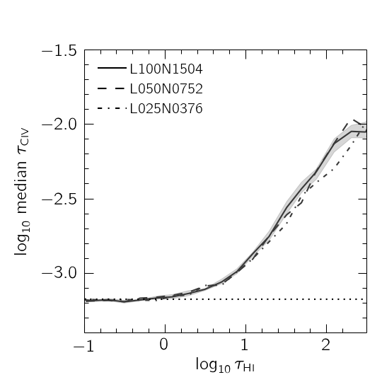
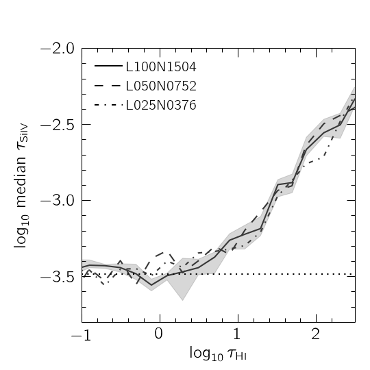
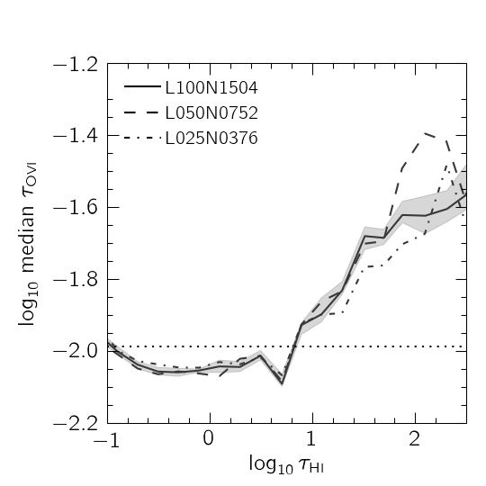
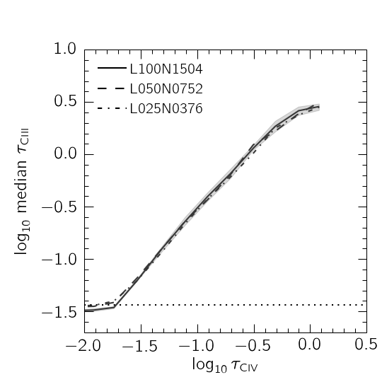
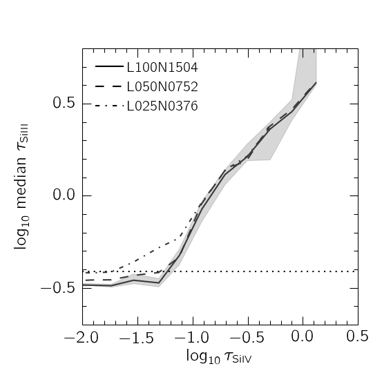
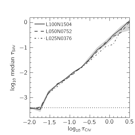
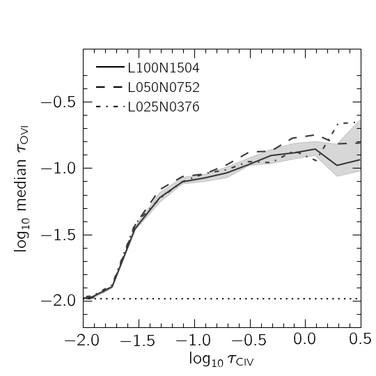
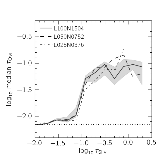
Figure 8: Convergence with respect to simulation box size, where we plot the same optical depth relations as were presented in Figs. 3, 5, and 6, but without combining different QSOs. For clarity, we only show the error region around the fiducial model (L100N1504), which was determined by bootstrap resampling the mock spectra. We find that our fiducial simulation is converged.

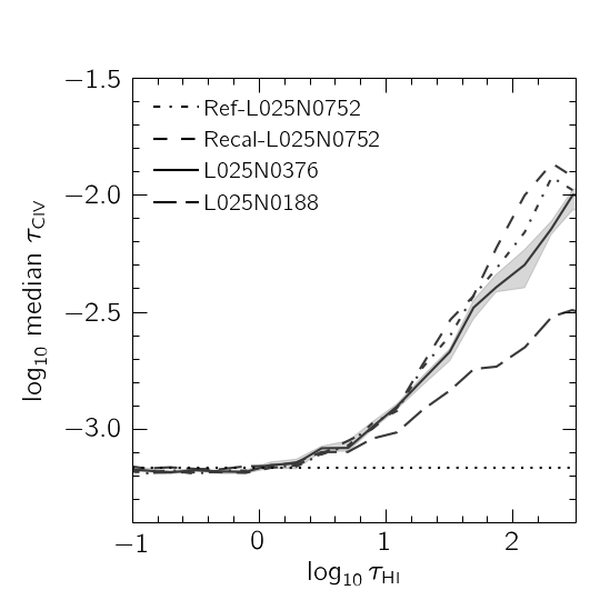
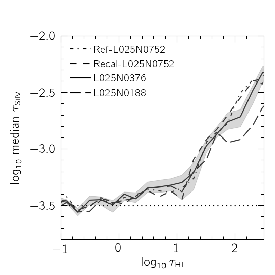
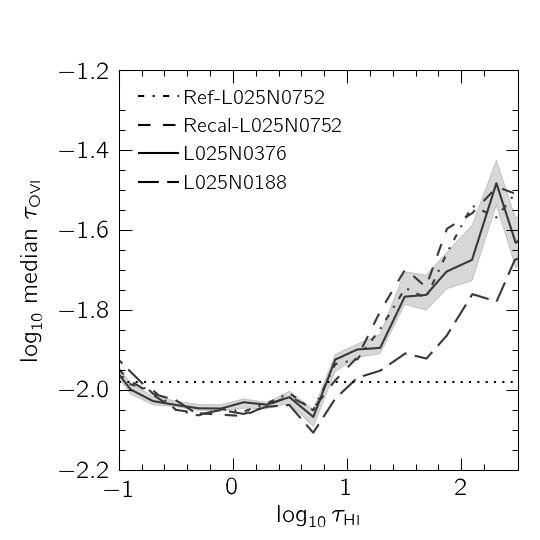
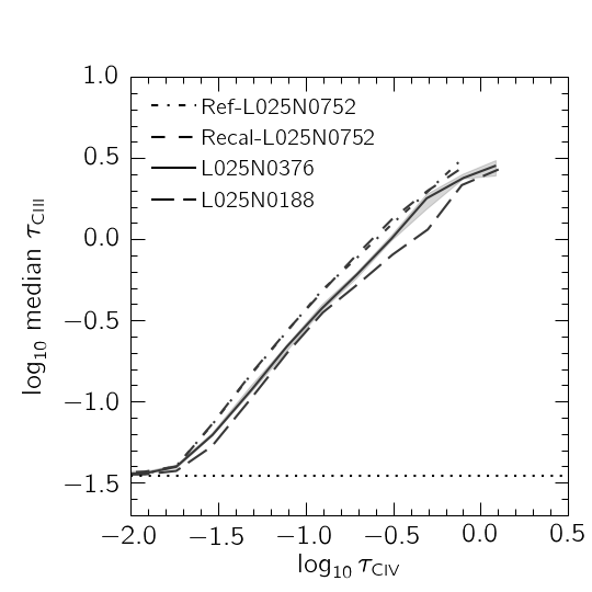
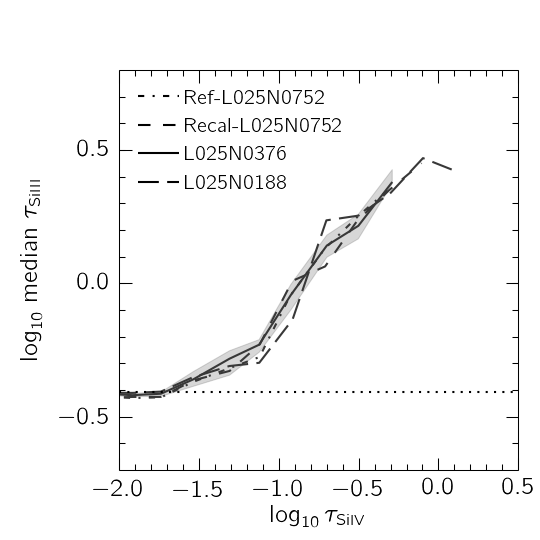
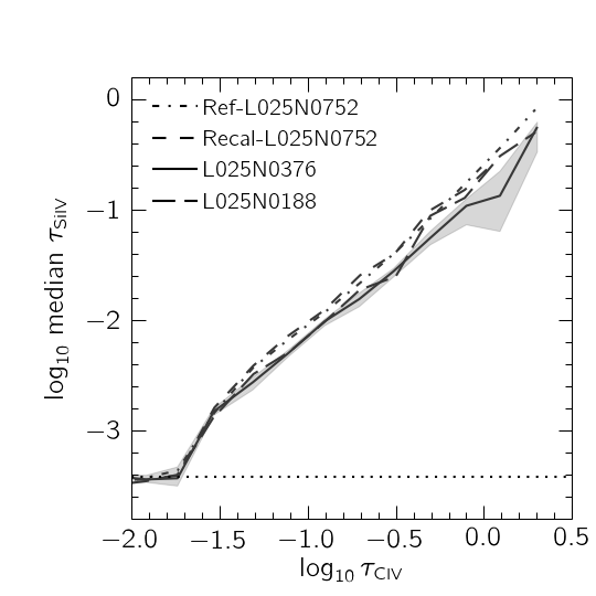
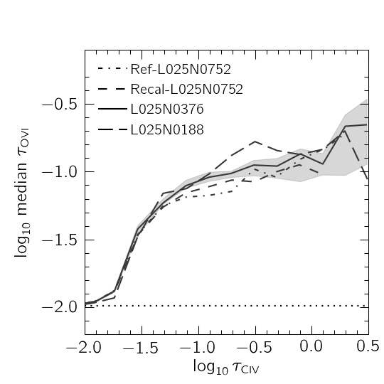
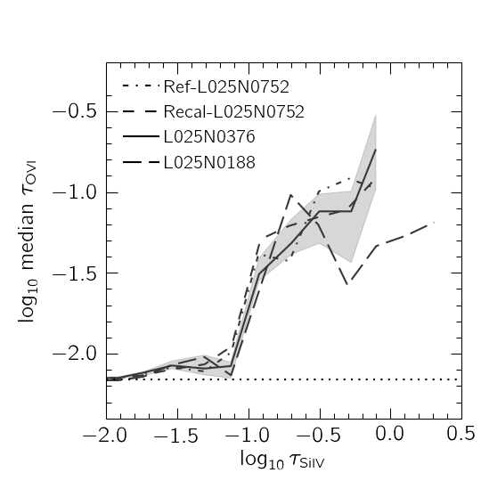
Figure 9: The same as Fig. 8, but showing convergence with respect to the numerical resolution and using a 25 cMpc box. Our fiducial resolution is given by the L025N0376 run, and indicated by the solid line and shaded error region. While the lowest-resolution run, Ref-L025N0188, deviates significantly from the others (especially for the Civ(Hi) relation), we find mostly good agreement between the fiducial intermediate- and high- resolution runs, which demonstrates that the fiducial resolution is nearly converged. However, the higher-resolution runs predict about 0.3 dex higher $\tau_{\rm C\textsc{iv}}^{\text{med}}$ at $\tau_{\rm H\textsc{i}}\approx 10^{2}$, which suggests that the Civ  and/or Hi associated with these rare, strong absorbers have not yet converged.

Appendix C Results from single QSOs

In this appendix, we present the pixel optical depth relations derived from individual QSOs, which were combined to obtain the relations shown in Figs. 3, 5, and 6. Here we display the optical depth relations in the same order as they appear in the paper: Civ(Hi) (Fig. 10), Siiv(Hi) (Fig. 11), Ovi(Hi) (Fig. 12), Ciii(Civ) (Fig. 13), Siiii(Siiv) (Fig. 14), Siiv(Civ) (Fig. 15), Ovi(Civ) (Fig. 16), and Ovi(Siiv) (Fig. 17).

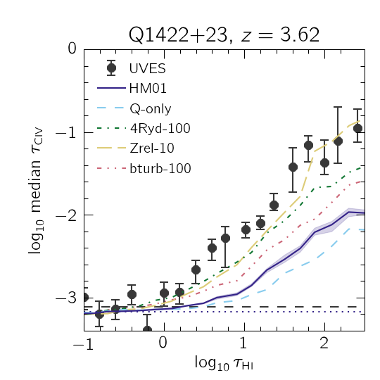
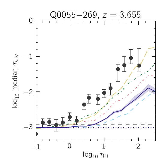
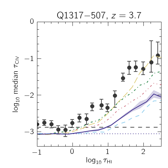
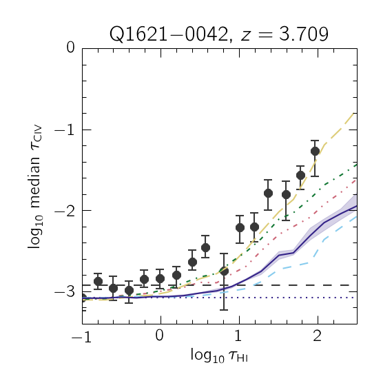
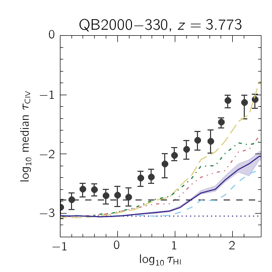
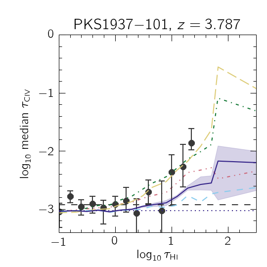
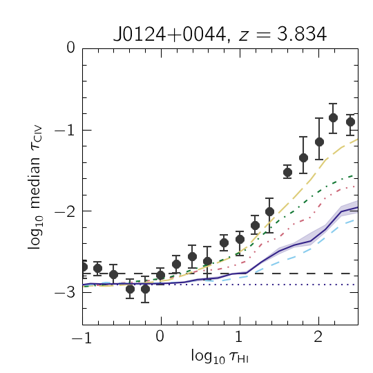
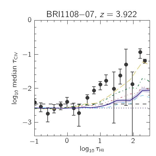
Figure 10: Median Civ optical depth in bins of $\tau_{\rm H\textsc{i}}$ for all eight QSOs. The black points represent the observed data, while the curves show results from simulated spectra created using different UVB models. The $1\sigma$ error bars on the observations were estimated by bootstrap resampling chunks of the spectrum, while the error regions shown for the fiducial simulation were calculated by bootstrap resampling the 100 mock spectra used to generate the data. The value of $\tau_{\text{min}}$ is indicated by the horizontal dashed line for the observations, and the horizontal dotted lines for the simulations.

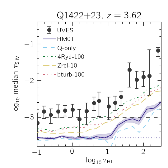
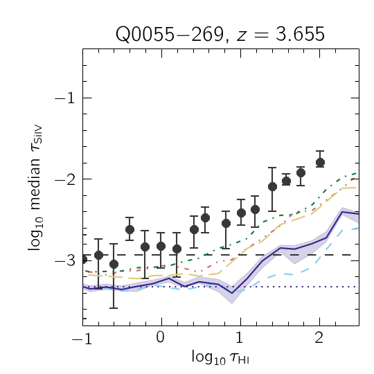
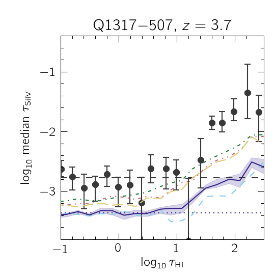
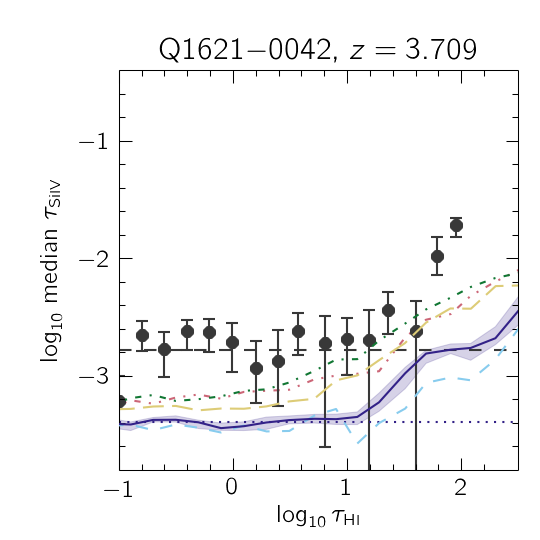
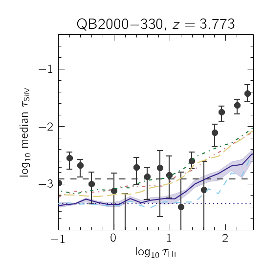
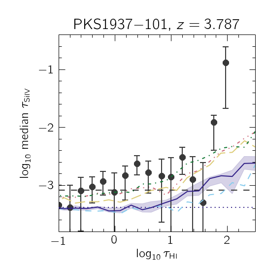
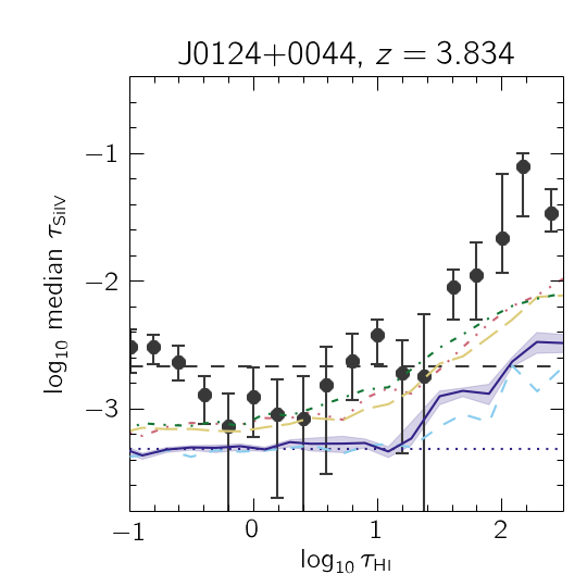
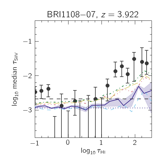
Figure 11: Same as Fig. 10, but for Siiv(Hi).

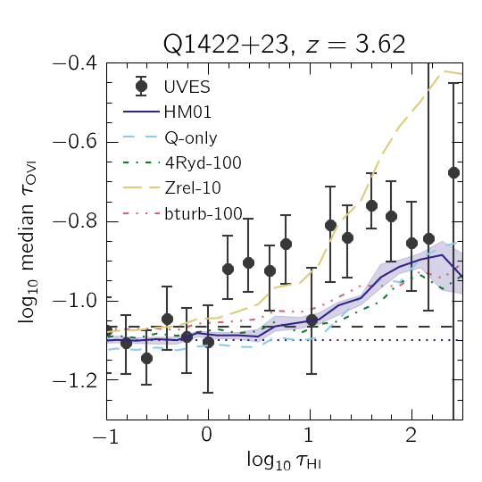
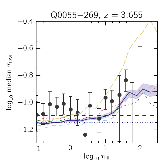
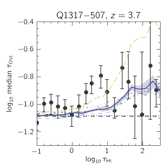
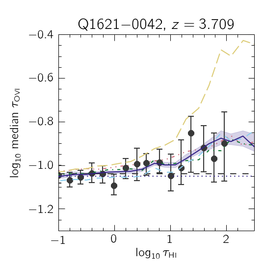
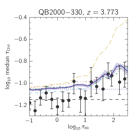
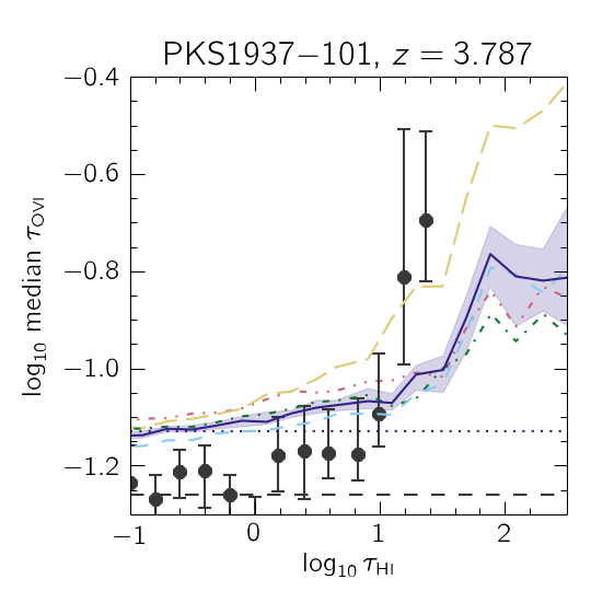
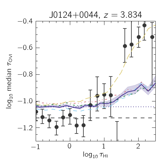
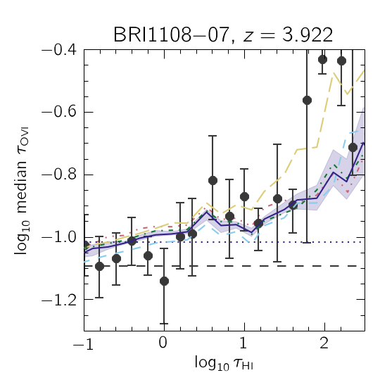
Figure 12: Same as Fig. 10, but for Ovi(Hi).

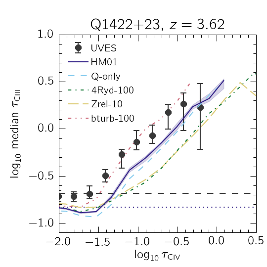
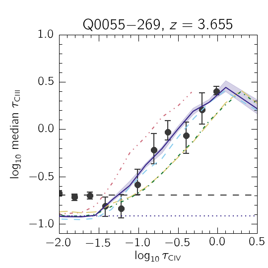
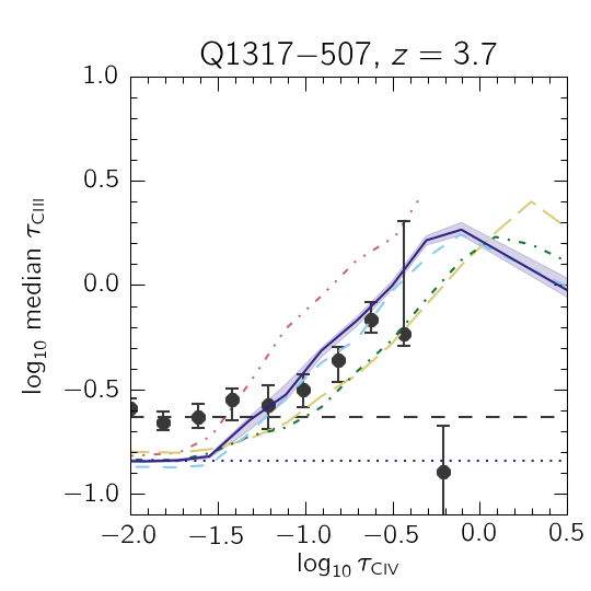
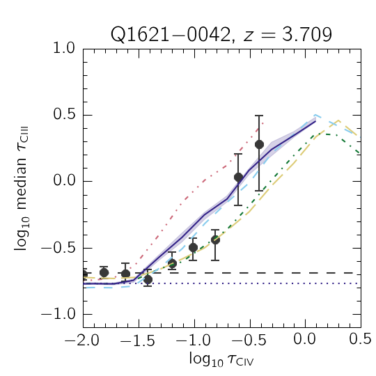
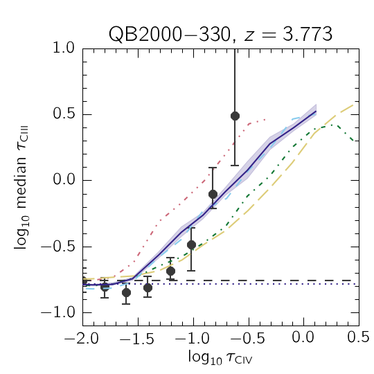
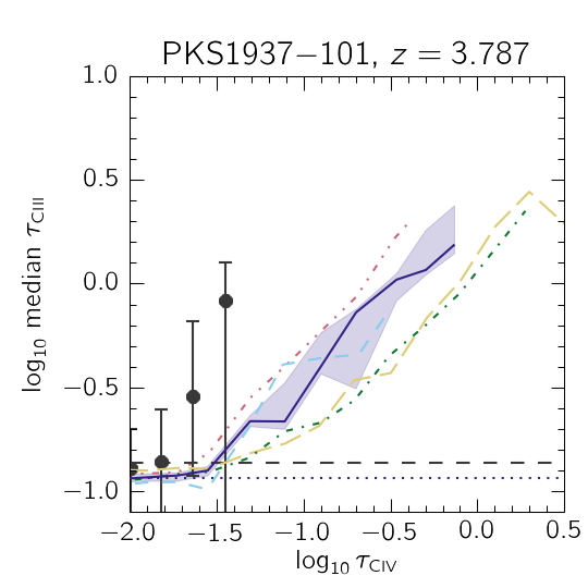
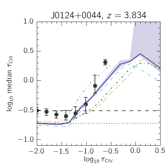
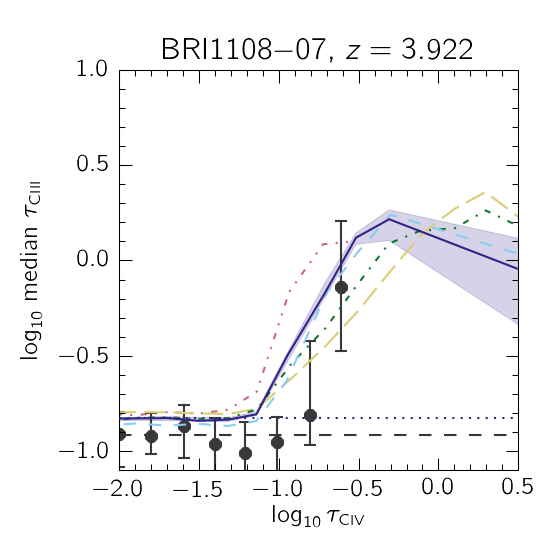
Figure 13: Same as Fig. 10, but for Ciii(Civ).

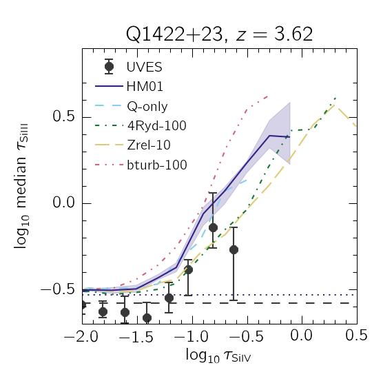
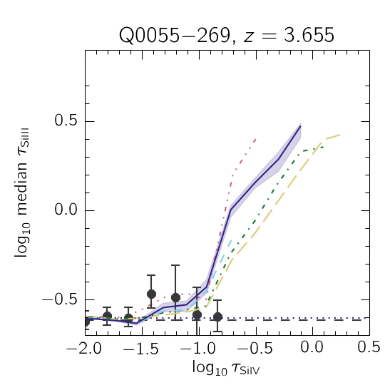
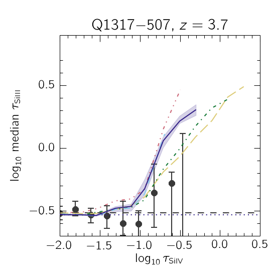
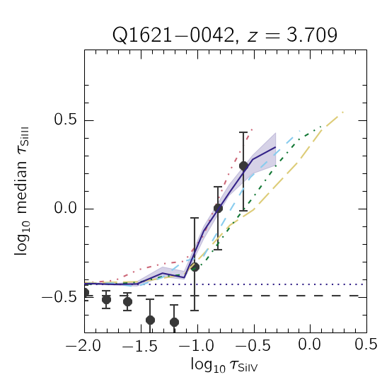
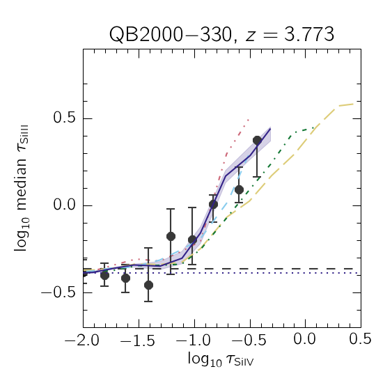
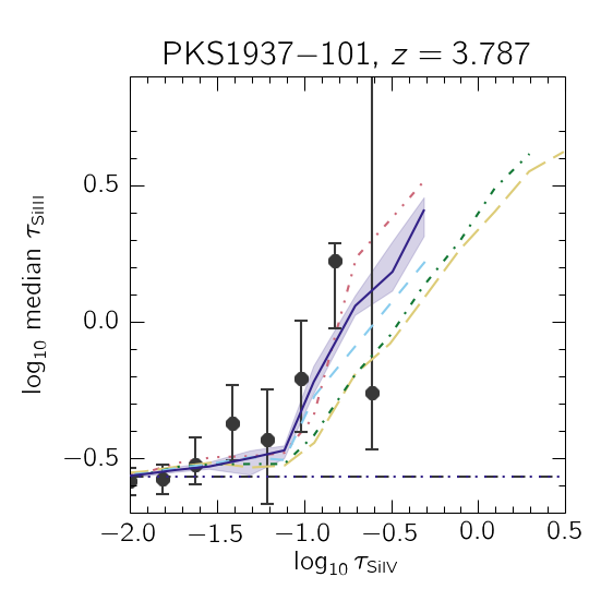
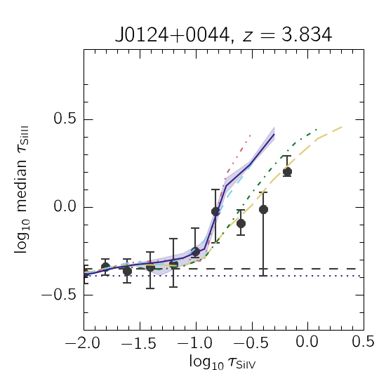
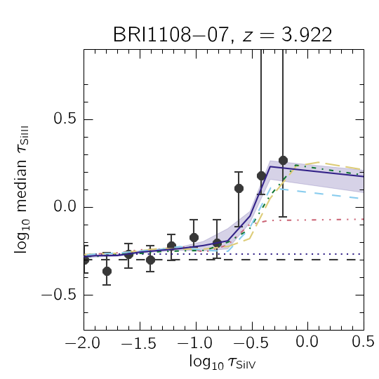
Figure 14: Same as Fig. 10, but for Siiii(Siiv).

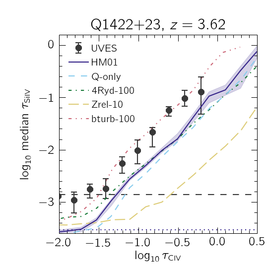
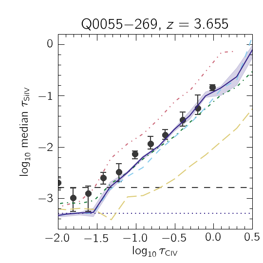
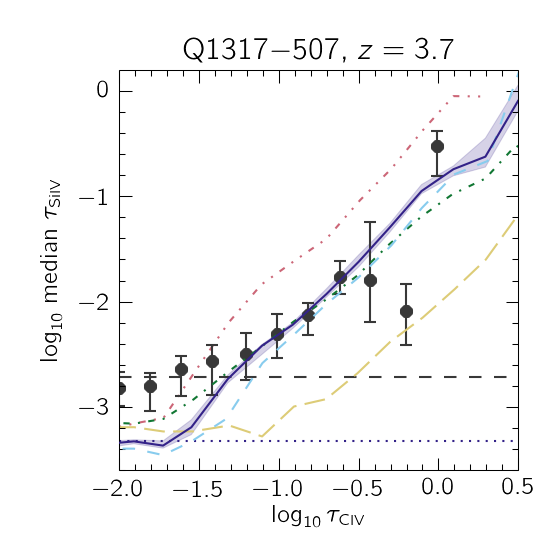
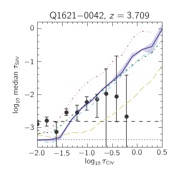
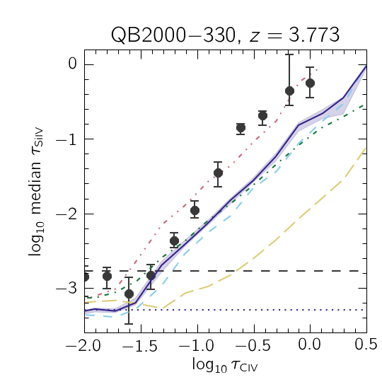
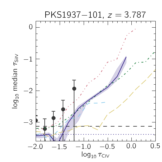
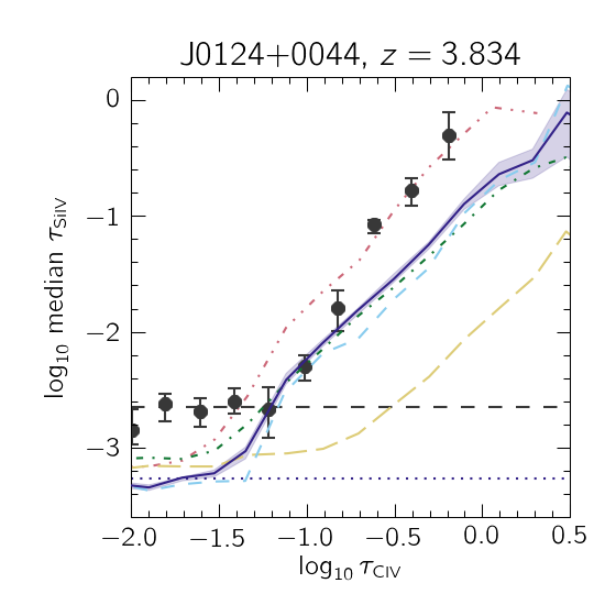
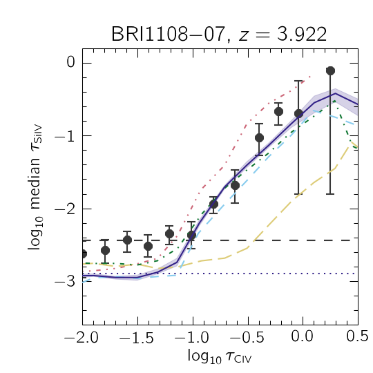
Figure 15: Same as Fig. 10, but for Siiv(Civ).

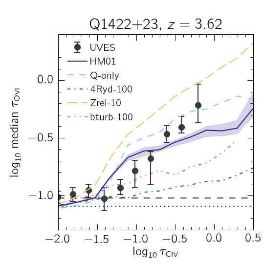
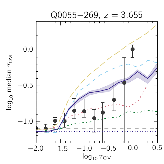
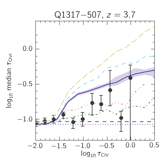
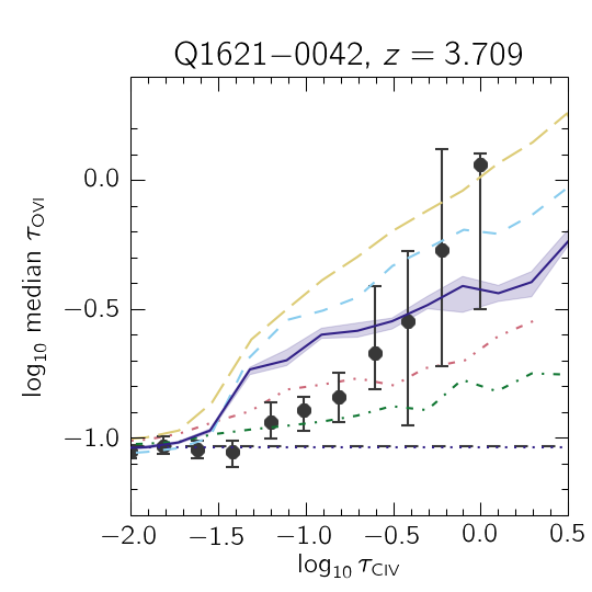
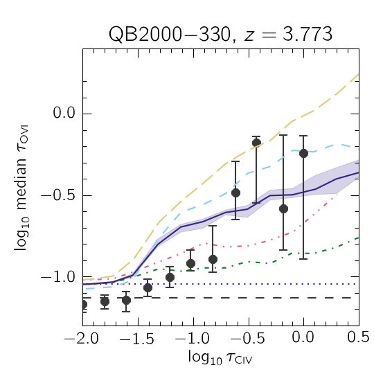
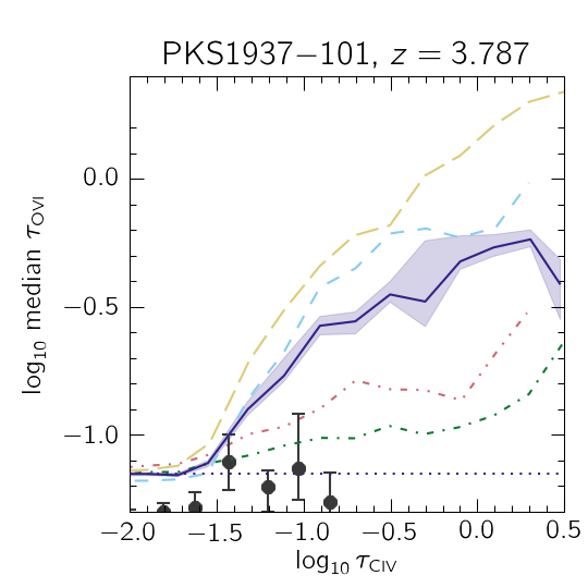
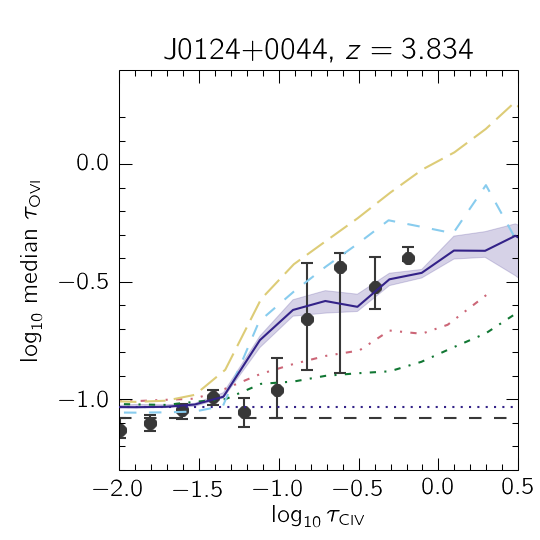
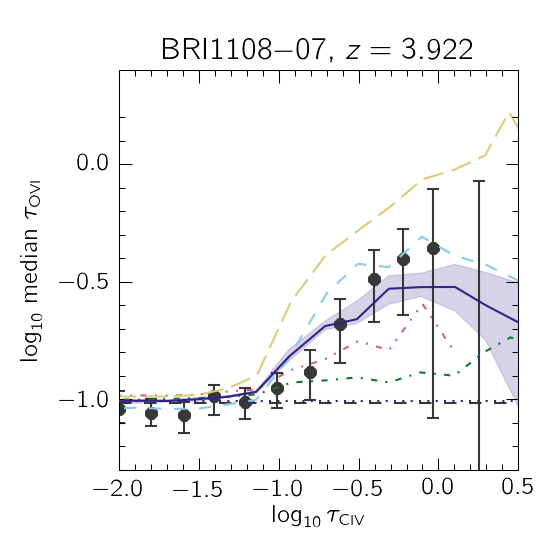
Figure 16: Same as Fig. 10, but for Ovi(Civ).

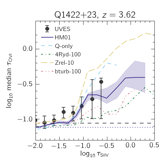
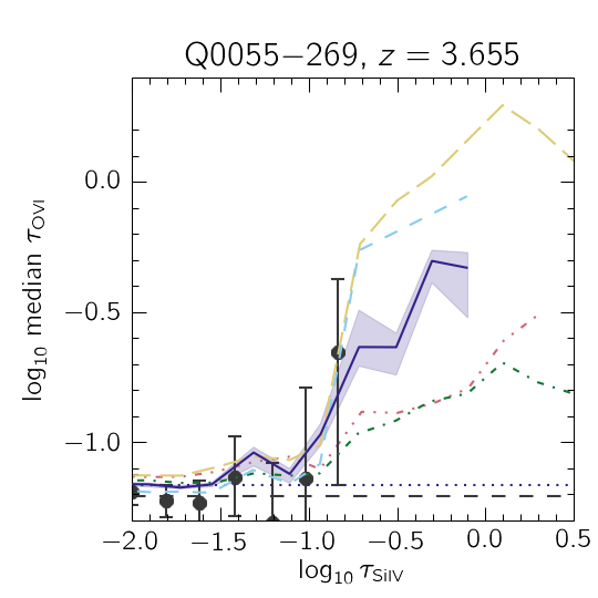
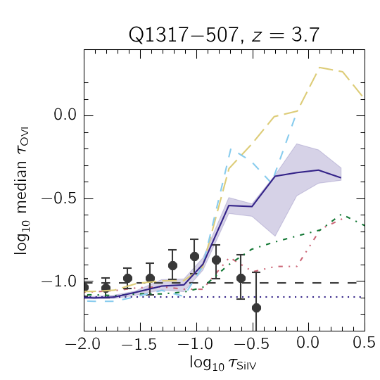
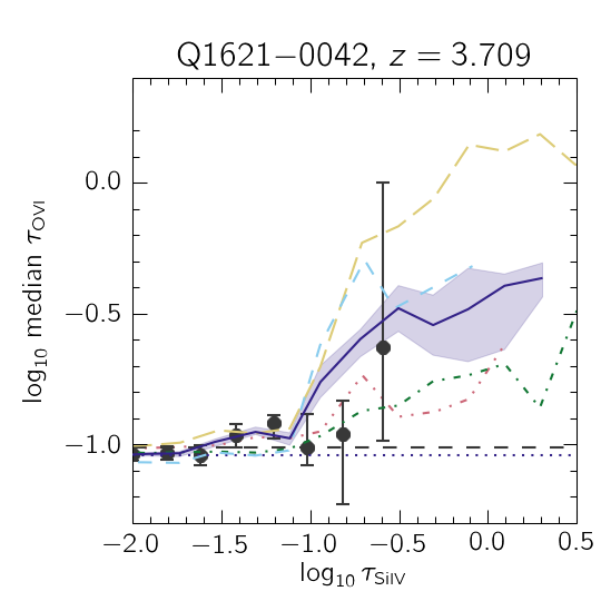
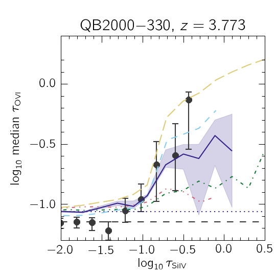
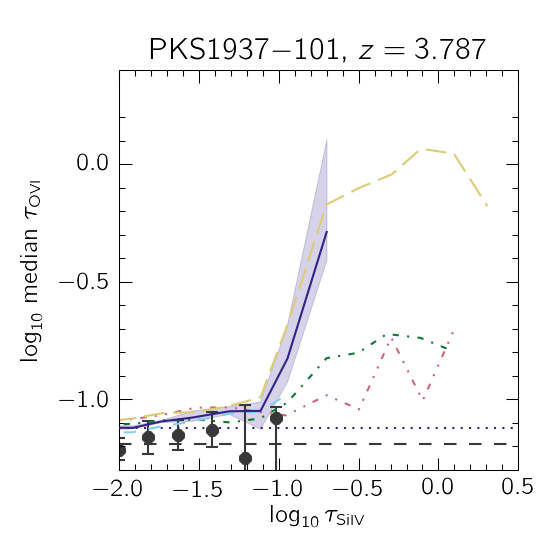
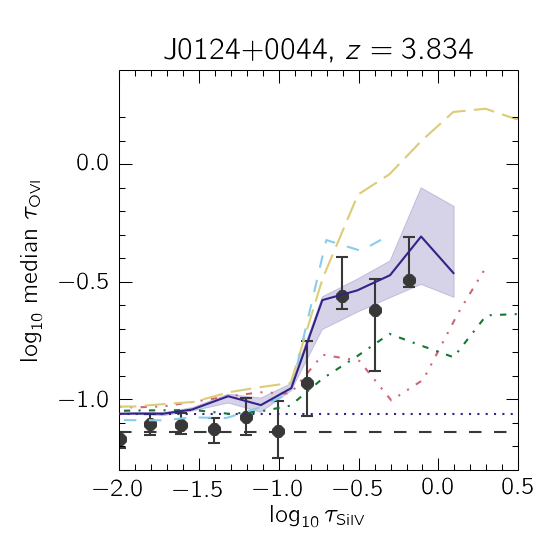
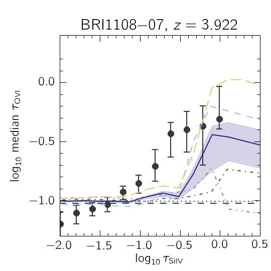
Figure 17: Same as Fig. 10, but for Ovi(Siiv).

References

- Aguirre et al. (2002) Aguirre A., Schaye J., Theuns T., 2002, ApJ, 576, 1
- Aguirre et al. (2004) Aguirre A., Schaye J., Kim T.-S., Theuns T., Rauch M., Sargent W. L. W., 2004, ApJ, 602, 38
- Aguirre et al. (2005) Aguirre A., Schaye J., Hernquist L., Kay S., Springel V., Theuns T., 2005, ApJ, 620, L13
- Aguirre et al. (2008) Aguirre A., Dow-Hygelund C., Schaye J., Theuns T., 2008, ApJ, 689, 851
- Becker et al. (2011) Becker G. D., Bolton J. S., Haehnelt M. G., Sargent W. L. W., 2011, MNRAS, 410, 1096
- Boksenberg & Sargent (2015) Boksenberg A., Sargent W. L. W., 2015, ApJS, 218, 7
- Boksenberg et al. (2003) Boksenberg A., Sargent W. L. W., Rauch M., 2003, ArXiv Astrophysics e-prints,
- Booth & Schaye (2009) Booth C. M., Schaye J., 2009, MNRAS, 398, 53
- Booth et al. (2012) Booth C. M., Schaye J., Delgado J. D., Dalla Vecchia C., 2012, MNRAS, 420, 1053
- Cowie & Songaila (1998) Cowie L. L., Songaila A., 1998, Nature, 394, 44
- Cowie et al. (1995) Cowie L. L., Songaila A., Kim T.-S., Hu E. M., 1995, AJ, 109, 1522
- Crain et al. (2015) Crain R. A., et al., 2015, MNRAS, 450, 1937
- Crain et al. (2016) Crain R. A., et al., 2016, preprint, (arXiv:1604.06803)
- Cullen & Dehnen (2010) Cullen L., Dehnen W., 2010, MNRAS, 408, 669
- D’Odorico et al. (2010) D’Odorico V., Calura F., Cristiani S., Viel M., 2010, MNRAS, 401, 2715
- Dalla Vecchia & Schaye (2012) Dalla Vecchia C., Schaye J., 2012, MNRAS, 426, 140
- Danforth & Shull (2008) Danforth C. W., Shull J. M., 2008, ApJ, 679, 194
- Durier & Dalla Vecchia (2012) Durier F., Dalla Vecchia C., 2012, MNRAS, 419, 465
- Ellison et al. (2000) Ellison S. L., Songaila A., Schaye J., Pettini M., 2000, AJ, 120, 1175
- Faucher-Giguère et al. (2009) Faucher-Giguère C.-A., Lidz A., Zaldarriaga M., Hernquist L., 2009, ApJ, 703, 1416
- Ferland et al. (2013) Ferland G. J., et al., 2013, Rev. Mexicana Astron. Astrofis., 49, 137
- Ford et al. (2013) Ford A. B., Oppenheimer B. D., Davé R., Katz N., Kollmeier J. A., Weinberg D. H., 2013, MNRAS, 432, 89
- Furlong et al. (2015a) Furlong M., et al., 2015a, preprint, (arXiv:1510.05645)
- Furlong et al. (2015b) Furlong M., et al., 2015b, MNRAS, 450, 4486
- Haardt & Madau (2001) Haardt F., Madau P., 2001, in Neumann D. M., Tran J. T. V., eds, Clusters of Galaxies and the High Redshift Universe Observed in X-rays. (arXiv:astro-ph/0106018)
- Haardt & Madau (2012) Haardt F., Madau P., 2012, ApJ, 746, 125
- Haas et al. (2013) Haas M. R., Schaye J., Booth C. M., Dalla Vecchia C., Springel V., Theuns T., Wiersma R. P. C., 2013, MNRAS, 435, 2931
- Hopkins (2013) Hopkins P. F., 2013, MNRAS, 428, 2840
- Kollmeier et al. (2014) Kollmeier J. A., et al., 2014, ApJ, 789, L32
- Lidz et al. (2010) Lidz A., Faucher-Giguère C.-A., Dall’Aglio A., McQuinn M., Fechner C., Zaldarriaga M., Hernquist L., Dutta S., 2010, ApJ, 718, 199
- Morton (2003) Morton D. C., 2003, ApJS, 149, 205
- Oppenheimer et al. (2016) Oppenheimer B. D., et al., 2016, MNRAS,
- Planck Collaboration et al. (2014) Planck Collaboration et al., 2014, A&A, 571, A16
- Price (2008) Price D. J., 2008, Journal of Computational Physics, 227, 10040
- Rahmati et al. (2013a) Rahmati A., Pawlik A. H., Raičevic̀ M., Schaye J., 2013a, MNRAS, 430, 2427
- Rahmati et al. (2013b) Rahmati A., Schaye J., Pawlik A. H., Raicevic M., 2013b, MNRAS, 431, 2261
- Rahmati et al. (2015) Rahmati A., Schaye J., Bower R. G., Crain R. A., Furlong M., Schaller M., Theuns T., 2015, MNRAS, 452, 2034
- Rahmati et al. (2016) Rahmati A., Schaye J., Crain R. A., Oppenheimer B. D., Schaller M., Theuns T., 2016, MNRAS,
- Rakic et al. (2012) Rakic O., Schaye J., Steidel C. C., Rudie G. C., 2012, ApJ, 751, 94
- Rosas-Guevara et al. (2015) Rosas-Guevara Y. M., et al., 2015, MNRAS, 454, 1038
- Rudie et al. (2012a) Rudie G. C., et al., 2012a, ApJ, 750, 67
- Rudie et al. (2012b) Rudie G. C., Steidel C. C., Pettini M., 2012b, ApJ, 757, L30
- Savage et al. (2014) Savage B. D., Kim T.-S., Wakker B. P., Keeney B., Shull J. M., Stocke J. T., Green J. C., 2014, ApJS, 212, 8
- Schaller et al. (2015) Schaller M., Dalla Vecchia C., Schaye J., Bower R. G., Theuns T., Crain R. A., Furlong M., McCarthy I. G., 2015, MNRAS, 454, 2277
- Schaye (2001) Schaye J., 2001, ApJ, 559, 507
- Schaye (2004) Schaye J., 2004, ApJ, 609, 667
- Schaye (2006) Schaye J., 2006, ApJ, 643, 59
- Schaye & Dalla Vecchia (2008) Schaye J., Dalla Vecchia C., 2008, MNRAS, 383, 1210
- Schaye et al. (2000a) Schaye J., Theuns T., Rauch M., Efstathiou G., Sargent W. L. W., 2000a, MNRAS, 318, 817
- Schaye et al. (2000b) Schaye J., Rauch M., Sargent W. L. W., Kim T.-S., 2000b, ApJ, 541, L1
- Schaye et al. (2003) Schaye J., Aguirre A., Kim T.-S., Theuns T., Rauch M., Sargent W. L. W., 2003, ApJ, 596, 768
- Schaye et al. (2015) Schaye J., et al., 2015, MNRAS, 446, 521
- Shen et al. (2013) Shen S., Madau P., Guedes J., Mayer L., Prochaska J. X., Wadsley J., 2013, ApJ, 765, 89
- Shull et al. (2010) Shull J. M., France K., Danforth C. W., Smith B., Tumlinson J., 2010, ApJ, 722, 1312
- Simcoe et al. (2004) Simcoe R. A., Sargent W. L. W., Rauch M., 2004, ApJ, 606, 92
- Songaila (2001) Songaila A., 2001, ApJ, 561, L153
- Songaila (2005) Songaila A., 2005, AJ, 130, 1996
- Springel (2005) Springel V., 2005, MNRAS, 364, 1105
- Springel et al. (2005) Springel V., Di Matteo T., Hernquist L., 2005, MNRAS, 361, 776
- Stinson et al. (2012) Stinson G. S., et al., 2012, MNRAS, 425, 1270
- Tepper-García et al. (2011) Tepper-García T., Richter P., Schaye J., Booth C. M., Dalla Vecchia C., Theuns T., Wiersma R. P. C., 2011, MNRAS, 413, 190
- Theuns et al. (1998) Theuns T., Leonard A., Efstathiou G., Pearce F. R., Thomas P. A., 1998, MNRAS, 301, 478
- Theuns et al. (2002) Theuns T., Viel M., Kay S., Schaye J., Carswell R. F., Tzanavaris P., 2002, ApJ, 578, L5
- Trayford et al. (2015) Trayford J. W., et al., 2015, MNRAS, 452, 2879
- Turner et al. (2014) Turner M. L., Schaye J., Steidel C. C., Rudie G. C., Strom A. L., 2014, MNRAS, 445, 794
- Turner et al. (2015) Turner M. L., Schaye J., Steidel C. C., Rudie G. C., Strom A. L., 2015, MNRAS, 450, 2067
- Véron-Cetty & Véron (2010) Véron-Cetty M.-P., Véron P., 2010, A&A, 518, A10
- Wendland (1994) Wendland H., 1994, Advances Comput. Math., 4, 389
- Wiersma et al. (2009a) Wiersma R. P. C., Schaye J., Smith B. D., 2009a, MNRAS, 393, 99
- Wiersma et al. (2009b) Wiersma R. P. C., Schaye J., Theuns T., Dalla Vecchia C., Tornatore L., 2009b, MNRAS, 399, 574
- Wiersma et al. (2010) Wiersma R. P. C., Schaye J., Dalla Vecchia C., Booth C. M., Theuns T., Aguirre A., 2010, MNRAS, 409, 132
- Worseck et al. (2011) Worseck G., et al., 2011, ApJ, 733, L24
- van de Voort et al. (2011) van de Voort F., Schaye J., Booth C. M., Haas M. R., Dalla Vecchia C., 2011, MNRAS, 414, 2458