A reduced model for precessional switching of thin-film nanomagnets under the influence of spin-torque

Abstract

We study the magnetization dynamics of thin-film magnetic elements with in-plane magnetization subject to a spin-current flowing perpendicular to the film plane. We derive a reduced partial differential equation for the in-plane magnetization angle in a weakly damped regime. We then apply this model to study the experimentally relevant problem of switching of an elliptical element when the spin-polarization has a component perpendicular to the film plane, restricting the reduced model to a macrospin approximation. The macrospin ordinary differential equation is treated analytically as a weakly damped Hamiltonian system, and an orbit-averaging method is used to understand transitions in solution behaviors in terms of a discrete dynamical system. The predictions of our reduced model are compared to those of the full Landau–Lifshitz–Gilbert–Slonczewski equation for a macrospin.

I Introduction

Magnetization dynamics in the presence of spin-transfer torques is a very active area of research with applications to magnetic memory devices and oscillators BaderParkin2010 ; BrataasKentOhno2012 ; KentWorledge2015 . Some basic questions relate to the types of magnetization dynamics that can be excited and the time scales on which the dynamics occurs. Many of the experimental studies of spin-transfer torques are on thin film magnetic elements patterned into asymmetric shapes (e.g. an ellipse) in which the demagnetizing field strongly confines the magnetization to the film plane. Analytic models that capture the resulting nearly in-plane magnetization dynamics (see e.g. GarciaCerveraE01 ; DKMO ; KohnSlas05Dynamics ; MuratovOsipov06 ; CapellaOttoMelcher ) can lead to new insights and guide experimental studies and device design. A macrospin model that treats the entire magnetization of the element as a single vector of fixed length is a starting point for most analyses.

The focus of this paper is on a thin-film magnetic element excited by a spin-polarized current that has an out-of-plane component. This out-of-plane component of spin-polarization can lead to magnetization precession about the film normal or magnetization reversal. The former dynamics would be desired for a spin-transfer torque oscillator, while the latter dynamics would be essential in a magnetic memory device. A device in which a perpendicular component of spin-polarization is applied to an in-plane magnetized element was proposed in Ref. [Kent2004, ] and has been studied experimentally Liu2010 ; Liu2012 ; Ye2015 . There have also been a number of models that have considered the influence of thermal noise on the resulting dynamics, e.g., on the rate of switching and the dephasing of the oscillator motion Newhall2013 ; Pinna2013 ; Pinna2014 .

Here we consider a weakly damped asymptotic regime of the Landau–Lifshitz–Gilbert–Slonczewski (LLGS) equation for a thin-film ferromagnet, in which the oscillatory nature of the in-plane dynamics is highlighted. In this regime, we derive a reduced partial differential equation (PDE) for the in-plane magnetization dynamics under applied spin-torque, which is a generalization of the underdamped wave-like model due to Capella, Melcher and Otto CapellaOttoMelcher . We then analyze the solutions of this equation under the macrospin (spatially uniform) approximation, and discuss the predictions of such a model in the context of previous numerical studies of the full LLGS equation ChavesKent15 .

The rest of this article is organized as follows. In Sec. II, we perform an asymptotic derivation of the reduced underdamped equation for the in-plane magnetization dynamics in a thin-film element of arbitrary cross section, by first making a thin-film approximation to the LLGS equation, then a weak-damping approximation. In Sec. III, we then further reduce to a macrospin ordinary differential equation (ODE) by spatial averaging of the underdamped PDE, and restrict to the particular case of a soft elliptical element. A brief parametric study of the ODE solutions is then presented, varying the spin-current parameters. In Sec. IV, we make an analytical study of the macrospin equation using an orbit-averaging method to reduce to a discrete dynamical system, and compare its predictions to the full ODE solutions. In Sec. V, we seek to understand transitions between the different solution trajectories (and thus predict current-parameter values when the system will either switch or precess) by studying the discrete dynamical system derived in Sec. IV. Finally, we summarize our findings in Sec. VI.

II Reduced model

We consider a domain $\Omega\subset\mathbb{R}^{3}$ occupied by a ferromagnetic film with cross-section $D\subset\mathbb{R}^{2}$ and thickness $d$, i.e., $\Omega=D\times(0,d)$. Under the influence of a spin-polarized electric current applied perpendicular to the film plane, the magnetization vector $\mathbf{m}=\mathbf{m}(\mathbf{r},t)$, with $|\mathbf{m}|=1$ in $\Omega$ and $0$ outside, satisfies the LLGS equation (in SI units)

$$\frac{\partial\mathbf{m}}{\partial t}=-\gamma\mu_{0}\mathbf{m}\times\mathbf{H}_{\text{eff}}+{\alpha}\mathbf{m}\times\frac{\partial\mathbf{m}}{\partial t}+{\tau_{\text{STT}}}$$ (1)

in $\Omega$, with ${\partial\mathbf{m}}/{\partial n}=(\mathbf{n}\cdot\nabla)\mathbf{m}=0$ on $\partial\Omega$, where $\mathbf{n}$ is the outward unit normal to $\partial\Omega$. In the above, $\alpha>0$ is the Gilbert damping parameter, $\gamma$ is the gyromagnetic ratio, $\mu_{0}$ is the permeability of free space, $\mathbf{H}_{\text{eff}}=-\frac{1}{\mu_{0}M_{s}}\frac{\delta E}{\delta\mathbf{m}}$ is the effective magnetic field,

$$E(\mathbf{m})=\int_{\Omega}\Big{(}A|\nabla\mathbf{m}|^{2}+K\Phi(\mathbf{m})-\mu_{0}M_{s}\mathbf{H}_{\text{ext}}\cdot\mathbf{m})\Big{)}\,\mathrm{d}^{3}r\\ +\mu_{0}M_{s}^{2}\int_{\mathbb{R}^{3}}\int_{\mathbb{R}^{3}}\frac{\nabla\cdot\mathbf{m}(\mathbf{r})\nabla\cdot\mathbf{m}(\mathbf{r^{\prime}})}{8\pi|\mathbf{r}-\mathbf{r}^{\prime}|}\,\mathrm{d}^{3}r\,\mathrm{d}^{3}r^{\prime}$$ (2)

is the micromagnetic energy with exchange constant $A$, anisotropy constant $K$, crystalline anisotropy function $\Phi$, external magnetic field $\mathbf{H}_{\text{ext}}$, and saturation magnetization $M_{s}$. Additionally, the Slonczewski spin-transfer torque $\tau_{\text{STT}}$ is given by

$$\tau_{\text{STT}}=-\frac{\eta\gamma\hbar j}{2deM_{s}}\mathbf{m}\times\mathbf{m}\times\mathbf{p},$$ (3)

where $j$ is the density of current passing perpendicularly through the film, $e$ is the elementary charge (positive), $\mathbf{p}$ is the spin-polarization direction, and $\eta\in(0,1]$ is the spin-polarization efficiency.

We now seek to nondimensionalize the above system. Let

$$\ell=\sqrt{\frac{2A}{\mu_{0}M_{s}^{2}}},\quad Q=\frac{2K}{\mu_{0}M_{s}^{2}},\quad\mathbf{h}_{\text{ext}}=\frac{\mathbf{H}_{\text{ext}}}{M_{s}}.$$ (4)

We then rescale space and time as

$$\mathbf{r}\to\ell\mathbf{r},\quad t\to\frac{t}{\gamma\mu_{0}M_{s}},$$ (5)

obtaining the nondimensional form

$$\frac{\partial\mathbf{m}}{\partial t}=-\mathbf{m}\times\mathbf{h}_{\text{eff}}+\alpha\mathbf{m}\times\frac{\partial\mathbf{m}}{\partial t}-\beta\mathbf{m}\times\mathbf{m}\times\mathbf{p},$$ (6)

where $\mathbf{h}_{\text{eff}}=\mathbf{H}_{\text{eff}}/M_{s}$, and

$$\beta=\frac{\eta\hbar j}{2de\mu_{0}M_{s}^{2}}$$ (7)

is the dimensionless spin-torque strength.

Since we are interested in thin films, we now assume that $\mathbf{m}$ is independent of the film thickness. Then, after rescaling

$$E\to\mu_{0}M_{s}^{2}d\ell^{2}E,$$ (8)

we have $\mathbf{h}_{\text{eff}}\simeq-\frac{\delta E}{\delta\mathbf{m}}$, where $E$ is given by a local energy functional defined on the (rescaled) two-dimensional domain $D$ (see, e.g., Ref. [KohnSlas05Gamma, ]):

$$E(\mathbf{m})\simeq\frac{1}{2}\int_{D}\left(|\nabla\mathbf{m}|^{2}+Q\Phi(\mathbf{m})-2\mathbf{h}_{\text{ext}}\cdot\mathbf{m}\right)\,\mathrm{d}^{2}r\\ +\frac{1}{2}\int_{D}m_{\perp}^{2}\,\mathrm{d}^{2}r+\frac{1}{4\pi}\delta|\ln\lambda|\int_{\partial D}(\mathbf{m}\cdot\mathbf{n})^{2}\,\mathrm{d}s,$$ (9)

in which now $\mathbf{m}:D\to\mathbb{S}^{2}$, $m_{\perp}$ is its out-of-plane component, $\delta=d/\ell$ is the dimensionless film thickness, and $\lambda=d/L\ll 1$ (where $L$ is the lateral size of the film) is the film’s aspect ratio. The effective field is given explicitly by

$$\mathbf{h}_{\text{eff}}=\Delta\mathbf{m}-\frac{Q}{2}\nabla_{\mathbf{m}}\Phi(\mathbf{m})-m_{\perp}\mathbf{e}_{z}+\mathbf{h}_{\text{ext}},$$ (10)

and $\mathbf{m}$ satisfies equation (6) in $D$ with the boundary condition

$$\frac{\partial\mathbf{m}}{\partial n}=-\frac{1}{2\pi}\delta|\ln\lambda|(\mathbf{m}\cdot\mathbf{n})(\mathbf{n}-(\mathbf{m}\cdot\mathbf{n})\,\mathbf{m})$$ (11)

on $\partial D$.

We now parametrize $\mathbf{m}$ in terms of spherical angles as

$$\mathbf{m}=(-\sin\theta\cos\phi,\cos\theta\cos\phi,\sin\phi),$$ (12)

and the current polarization direction $\mathbf{p}$ in terms of an in-plane angle $\psi$ and its out-of-plane component $p_{\perp}$ as

$$\mathbf{p}=\frac{1}{\sqrt{1+p_{\perp}^{2}}}(-\sin\psi,\cos\psi,p_{\perp}).$$ (13)

Writing ${\beta}_{*}={\beta}/\sqrt{1+p_{\perp}^{2}}$, after some algebra, one may then write equation (6) as the system

$$\frac{\partial\phi}{\partial t}=-\frac{1}{\cos\phi}\mathbf{h}_{\text{eff}}\cdot\mathbf{m}_{\theta}+\alpha\cos\phi\frac{\partial\theta}{\partial t}\\ +{\beta}_{*}(p_{\perp}\cos\phi-\sin\phi\cos(\theta-\psi)),$$ (14)

$$-\cos\phi\frac{\partial\theta}{\partial t}=-\mathbf{h}_{\text{eff}}\cdot\mathbf{m}_{\phi}+\alpha\frac{\partial\phi}{\partial t}+{\beta}_{*}\sin(\theta-\psi),$$ (15)

where $\mathbf{m}_{\theta}=\partial\mathbf{m}/\partial\theta$ and $\mathbf{m}_{\phi}=\partial\mathbf{m}/\partial\phi$ for $\mathbf{m}$ given by (12). Again, since we are working in a soft thin film, we assume $\phi\ll 1$ and that the out-of-plane component of the effective field in equation (10) is dominated by the term $\mathbf{h}_{\text{eff}}\cdot\mathbf{e}_{z}\simeq-m_{\perp}=-\sin\phi$. Note that this assumes that the crystalline anisotropy and external field terms in the out-of-plane directions are relatively small, so we assume the external field is only in plane, though it is still possible to include a perpendicular anisotropy simply by renormalizing the constant in front of the $m_{\perp}$ term in $\mathbf{h}_{\text{eff}}$. We then linearize the above system in $\phi$, yielding

$$\frac{\partial\phi}{\partial t}=\frac{\delta\mathcal{E}}{\delta\theta}+\alpha\frac{\partial\theta}{\partial t}+{\beta}_{*}(p_{\perp}-\phi\cos(\theta-\psi)),$$ (16)

$$-\frac{\partial\theta}{\partial t}=\phi+{\beta}_{*}\sin(\theta-\psi)\\ +\phi(-h_{x}\sin\theta+h_{y}\cos\theta)+\alpha\frac{\partial\phi}{\partial t}.$$ (17)

where $h_{x}=\mathbf{h}_{\text{eff}}\cdot\mathbf{e}_{x}$ and $h_{y}=\mathbf{h}_{\text{eff}}\cdot\mathbf{e}_{y}$, and $\mathcal{E}(\theta)$ is $E(\mathbf{m})$ evaluated at $\phi=0$.

We now note that the last two terms in (17) are negligible relative to $\phi$ whenever $|h_{x}|,|h_{y}|$ and $\alpha$ are small, which is true of typical clean thin-film samples of sufficiently large lateral extent. Neglecting these terms, one has

$$\frac{\partial\phi}{\partial t} =\frac{\delta\mathcal{E}}{\delta\theta}+\alpha\frac{\partial\theta}{\partial t}+\beta_{*}(p_{\perp}-\phi\cos(\theta-\psi)),$$ (18)

$$-\frac{\partial\theta}{\partial t} =\beta_{*}\sin(\theta-\psi)+\phi.$$ (19)

Then, differentiating (19) with respect to $t$ and using the result along with (19) to eliminate $\phi$ and $\frac{\partial\phi}{\partial t}$ from (18), we find a second-order in time equation for $\theta$:

$$0=\frac{\partial^{2}\theta}{\partial t^{2}}+\frac{\partial\theta}{\partial t}(\alpha+2\beta_{*}\cos(\theta-\psi))+\frac{\delta\mathcal{E}}{\delta\theta}\\ +\beta_{*}p_{\perp}+\beta_{*}^{2}\sin(\theta-\psi)\cos(\theta-\psi),$$ (20)

where, explicitly, one has

$$\frac{\delta\mathcal{E}}{\delta\theta}=-\Delta\theta+\frac{Q}{2}{\tilde{\Phi}^{\prime}}(\theta)+\mathbf{h}_{\text{ext}}\cdot(\cos\theta,\sin\theta),$$ (21)

and $\tilde{\Phi}(\theta)=\Phi(\mathbf{m}(\theta))$. In turn, from the boundary condition on $\mathbf{m}$ in (11), we can derive the boundary condition for $\theta$ as

$$\mathbf{n}\cdot\nabla\theta=\frac{1}{2\pi}\delta|\ln\lambda|\sin(\theta-\varphi)\cos(\theta-\varphi),$$ (22)

where $\varphi$ is the angle parametrizing the normal $\mathbf{n}$ to $\partial D$ via $\mathbf{n}=(-\sin\varphi,\cos\varphi)$.

The model comprised of (20)–(22) is a damped-driven wave-like PDE for $\theta$, which coincides with the reduced model of Ref. [CapellaOttoMelcher, ] for vanishing spin-current density in an infinite sample. This constitutes our reduced PDE model for magnetization dynamics in thin-film elements under the influence of out-of-plane spin currents. It is easy to see that all of the terms in (20) balance when the parameters are chosen so as to satisfy

$$\beta_{*}\sim p_{\perp}\sim\alpha\sim{Q}^{1/2}\sim|\mathbf{h}_{\text{ext}}|^{1/2}\sim\frac{\ell}{L}\sim\delta|\ln\lambda|.$$ (23)

This shows that it should be possible to rigorously obtain the reduced model in (20)–(22) in the asymptotic limit of $L\to\infty$ and $\alpha,\beta_{*},p_{\perp},Q,|\mathbf{h}_{\mathrm{ext}}|,\delta\to 0$ jointly, so that (23) holds.

III Macrospin switching

In this section we study the behavior of the reduced model (20)–(22) in the approximation that the magnetization is spatially uniform on an elliptical domain, and compare the solution phenomenology to that found by simulating the LLGS equation in the same physical situation, as studied in Ref. [ChavesKent15, ].

III.1 Derivation of macrospin model

Integrating equation (20) over the domain $D$ and using the boundary condition (22), we have

$$\int_{D}\left(\frac{\partial^{2}\theta}{\partial t^{2}}+\frac{\partial\theta}{\partial t}(\alpha+2\beta_{*}\cos(\theta-\psi))\right.\\ \left.+\beta_{*}p_{\perp}+\beta_{*}^{2}\sin(\theta-\psi)\cos(\theta-\psi)\right.\\ \left.+\frac{Q}{2}{\tilde{\Phi}^{\prime}}(\theta)+\mathbf{h}_{\text{ext}}\cdot(\cos\theta,\sin\theta)\right)\,\mathrm{d}^{2}r\\ =\frac{1}{2\pi}\delta|\ln\lambda|\int_{\partial D}\sin(\theta-\varphi)\cos(\theta-\varphi)\,\mathrm{d}s.$$ (24)

Assume now that $\theta$ does not vary appreciably across the domain $D$, which makes sense in magnetic elements that are not too large. This allows us to replace $\theta(\mathbf{r},t)$ by its spatial average $\bar{\theta}(t)=\frac{1}{|D|}\int_{D}\theta(\mathbf{r},t)\,\mathrm{d}^{2}r$, where $|D|$ stands for the area of $D$ in the units of $\ell^{2}$. Denoting time derivatives by overdots, and omitting the bar on $\bar{\theta}$ for notational simplicity, this spatial averaging leads to the following ODE for $\theta(t)$:

$$\ddot{\theta}+\dot{\theta}\left(\alpha+2\beta_{*}\cos(\theta-\psi)\right)+\beta_{*}^{2}\sin(\theta-\psi)\cos(\theta-\psi)\\ +\beta_{*}p_{\perp}+\frac{Q}{2}{\tilde{\Phi}^{\prime}}(\theta)+\mathbf{h}_{\text{ext}}\cdot(\cos\theta,\sin\theta)\\ =\frac{\delta|\ln\lambda|}{4\pi|D|}\,\sin 2\theta\int_{\partial D}\cos(2\varphi)\,\mathrm{d}s\\ -\frac{\delta|\ln\lambda|}{4\pi|D|}\,\cos 2\theta\int_{\partial D}\sin(2\varphi)\,\mathrm{d}s.$$ (25)

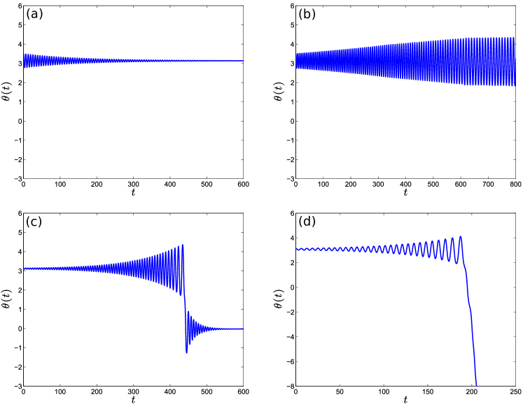
Figure 1: Solutions of macrospin equation (30) for $\alpha=0.01$, $\Lambda=0.1$. In (a), $p_{\perp}=0.2$, $\sigma=0.03$: decaying solution; in (b), $p_{\perp}=0.2$, $\sigma=0.06$: limit cycle solution (the initial conditions in (a) and (b) are $\theta(0)=3.5$, to better visualize the behavior). In (c), $p_{\perp}=0.3$, $\sigma=0.08$: switching solution; in (d), $p_{\perp}=0.6$, $\sigma=0.1$: precessing solution.

Next, we consider a particular physical situation in which to study the macrospin equation, motivated by previous work Liu2010 ; Liu2012 . As in Refs. [Pinna2013, ; Pinna2014, ; ChavesKent15, ], we consider an elliptical thin-film element (recall that lengths are now measured in the units of $\ell$):

$$D=\left\{(x,y)\ :\ {x^{2}\over a^{2}}+{y^{2}\over b^{2}}<1\right\},$$ (26)

with no in-plane crystalline anisotropy, $Q=0$, and no external field, $\mathbf{h}_{\text{ext}}=0$. We take the long axis of the ellipse to be aligned with the $\mathbf{e}_{y}$-direction, i.e. $b>a$, with the in-plane component of current polarization also aligned along this direction, i.e., taking $\psi=0$. One can then compute the integral over the boundary in equation (25) explicitly, leading to the equation

$$\ddot{\theta}+\dot{\theta}\left(\alpha+\beta_{*}\cos\theta\right)+\Lambda\sin\theta\cos\theta\\ +\beta_{*}^{2}\sin\theta\cos\theta+\beta_{*}p_{\perp}=0,$$ (27)

where we introduced the geometric parameter $0<\Lambda\ll 1$ obtained by an explicit integration:

$$\Lambda=\frac{\delta|\ln\lambda|}{2\pi^{2}ab}\int_{0}^{2\pi}\frac{b^{2}\cos^{2}\tau-a^{2}\sin^{2}\tau}{\sqrt{b^{2}\cos^{2}\tau+a^{2}\sin^{2}\tau}}\,\mathrm{d}\tau.$$ (28)

This may be computed in terms of elliptic integrals, though the expression is cumbersome so we omit it here. Importantly, up to a factor depending only on the eccentricity the value of $\Lambda$ is given by

$$\Lambda\sim\frac{d}{L}\ln\frac{L}{d}.$$ (29)

For example, for an elliptical nanomagnet with dimensions $100\times 30\times 2.5$ nm (similar to those considered in Ref. [ChavesKent15, ]), this yields $\Lambda\simeq 0.1$.

It is convenient to rescale time by $\sqrt{\Lambda}$ and divide through by $\Lambda$, yielding

$$\ddot{\theta}+\frac{1}{\sqrt{\Lambda}}\dot{\theta}\left(\alpha+2\sigma\Lambda\cos\theta\right)+\sin\theta\cos\theta\\ +\sigma p_{\perp}+\sigma^{2}\Lambda\sin\theta\cos\theta=0,$$ (30)

where we introduced $\sigma=\beta_{*}/\Lambda$. We then apply this ODE to model the problem of switching of the thin-film elements, taking the initial in-plane magnetization direction to be static and aligned along the easy axis, antiparallel to the in-plane component of the spin-current polarization. Thus, we take

$$\theta(0)=\pi,\quad\dot{\theta}(0)=0,$$ (31)

and study the resulting initial value problem.

III.2 Solution phenomenology

Let us briefly investigate the solution phenomenology as the dimensionless spin-current parameters $\sigma$ and $p_{\perp}$ are varied, with the material parameters, $\alpha$ and $\Lambda$, fixed. We take all parameters to be constant in time for simplicity. We find, by numerical integration, 4 types of solution to the initial value problem defined above. The sample solution curves are displayed in Fig. 1 below. The first (panel (a)) occurs for small values of $\sigma$, and consists simply of oscillations of $\theta$ around a fixed point close to the long axis of the ellipse, which decay in amplitude towards the fixed point, without switching.

Secondly (panel (b)), still below the switching threshold, the same oscillations about the fixed point can reach a finite fixed amplitude and persist without switching. This behavior corresponds to the onset of relatively small amplitude limit-cycle oscillations around the fixed point.

Thirdly (panel (c)), increasing either $\sigma,p_{\perp}$ or both, we obtain switching solutions. These have initial oscillations in $\theta$ about the fixed point near $\pi$, which increase in amplitude, and eventually cross the short axis of the ellipse at $\theta=\pi/2$. Then $\theta$ oscillates about the fixed point near 0, and the oscillations decay in amplitude toward the fixed point.

Finally (panel (d)), further increasing $\sigma$ and $p_{\perp}$ we obtain precessing solutions. Here, the initial oscillations about the fixed point near $\pi$ quickly grow to cross $\pi/2$, after which $\theta$ continues to decrease for all $t$, the magnetization making full precessions around the out-of-plane axis.

IV Half-period orbit-averaging approach

We now seek to gain some analytical insight into the transitions between the solution types discussed above. We do this by averaging over half-periods of the oscillations observed in the solutions to generate a discrete dynamical system which describes the evolution of the energy of a solution $\theta(t)$ on half-period time intervals.

Firstly, we observe that in the relevant parameter regimes the reduced equation (30) can be seen as a weakly perturbed Hamiltonian system. We consider both $\alpha$ and $\Lambda$ small, with $\alpha\lesssim\sqrt{\Lambda}$, and assume $\sigma\sim\alpha/\Lambda$ and $\sigma p_{\perp}\lesssim 1$. The arguments below can be rigorously justified by considering, for example, the limit $\Lambda\to 0$ while assuming that $\alpha=O(\Lambda)$ and that the values of $\sigma$ and $p_{\perp}$ are fixed. This limit may be achieved in the original model by sending jointly $d\to 0$ and $L\to\infty$, while keepingKohnSlas05Gamma

$${Ld\over\ell^{2}}\ln{L\over d}\lesssim 1.$$ (32)

The last condition ensures the consistency of the assumption that $\theta$ does not vary appreciably throughout $D$.

Introducing $\omega(t)=\dot{\theta}(t)$, (30) can be written to leading order as

$$\dot{\theta}=\frac{\partial\mathcal{H}}{\partial\omega},\quad\dot{\omega}=-\frac{\partial\mathcal{H}}{\partial\theta},$$ (33)

where we introduced

$$\mathcal{H}=\frac{1}{2}\omega^{2}+V(\theta),\quad V(\theta)=\frac{1}{2}{\sin^{2}\theta}+{\sigma p_{\perp}\theta}.$$ (34)

At the next order, the effects of finite $\alpha$ and $\Lambda$ appear in the first-derivative term in (30), while the other forcing term is still higher order. The behavior of (30) is therefore that of a weakly damped Hamiltonian system with Hamiltonian $\mathcal{H}$, with the effects of $\alpha$ and $\sigma$ serving to slowly change the value of $\mathcal{H}$ as the system evolves. Thus, we now employ the technique of orbit-averaging to reduce the problem further to the discrete dynamics of $\mathcal{H}(t)$, where the discrete time-steps are equal (to the leading order) to half-periods of the underlying Hamiltonian dynamics (which thus vary with $\mathcal{H}$).

Let us first compute the continuous-in-time dynamics of $\mathcal{H}$. From (34),

$$\dot{\mathcal{H}}=\omega(\dot{\omega}+V^{\prime}(\theta)),$$ (35)

which vanishes to leading order. At the next order, from (30), one has

$$\dot{\mathcal{H}}=-\frac{\omega^{2}}{\sqrt{\Lambda}}(\alpha+2\sigma\Lambda\cos\theta).$$ (36)

We now seek to average this dynamics over the Hamiltonian orbits. The general nature of the Hamiltonian orbits is either oscillations around a local minimum of $V(\theta)$ (limit cycles) or persistent precessions. If the local minimum of $V$ is close to an even multiple of $\pi$, $\mathcal{H}$ cannot increase, while if it is close to an odd multiple then $\mathcal{H}$ can increase if $\sigma$ is large enough. The switching process involves moving from the oscillatory orbits close to one of these odd minima, up the energy landscape, then jumping to oscillatory orbits around the neighboring even minimum, and decreasing in energy towards the new local fixed point.

We focus first on the oscillatory orbits. We may define their half-periods as

$$T(\mathcal{H})=\int_{\theta^{*}_{-}}^{\theta^{*}_{+}}\frac{\,\mathrm{d}\theta}{\dot{\theta}},$$ (37)

where $\theta_{-}^{*}$ and $\theta_{+}^{*}$ are the roots of the equation $V(\theta)=\mathcal{H}$ to the left and right of the local minimum of $V(\theta)$ about which $\theta(t)$ oscillates. To compute this integral, we assume that ${\theta(t)}$ follows the Hamiltonian trajectory:

$$\dot{\theta}=\pm\sqrt{2(\mathcal{H}-V(\theta))}.$$ (38)

We then define the half-period average of a function $f(\theta(t))$ as

$$\left<f\right>=\frac{1}{T(\mathcal{H})}\int_{\theta^{*}_{-}}^{\theta^{*}_{+}}\frac{f(\theta)\,\mathrm{d}\theta}{\sqrt{2(\mathcal{H}-V(\theta))}},$$ (39)

which agrees with the time average over half-period to the leading order. Note that this formula applies irrespectively of whether the trajectory connects $\theta^{*}_{-}$ to $\theta^{*}_{+}$ or $\theta^{*}_{+}$ to $\theta^{*}_{-}$. Applying this averaging to $\dot{\mathcal{H}}$, we then have

$$\left<\dot{\mathcal{H}}\right>=-\frac{1}{T(\mathcal{H})}\int_{\theta^{*}_{-}}^{\theta^{*}_{+}}\chi(\theta,\mathcal{H})\,\mathrm{d}\theta,$$ (40)

where we defined

$$\chi(\theta,\mathcal{H})=\frac{\left(\alpha+2\sigma\Lambda\cos\theta\right)\sqrt{2(\mathcal{H}-V(\theta))}}{\sqrt{\Lambda}}.$$ (41)

If the value of $\mathcal{H}$ is such that either of the roots $\theta^{*}_{\pm}$ no longer exist, this indicates that the system is now on a precessional trajectory. In order to account for this, we can define the period on a precessional trajectory instead as

$$T(\mathcal{H})=\int_{\theta_{C}-\pi}^{\theta_{C}}\frac{\,\mathrm{d}\theta}{\dot{\theta}},$$ (42)

where $\theta_{C}$ is a local maximum of $V(\theta)$. On the precessional trajectories, we then have

$$\left<\dot{\mathcal{H}}\right>=-\frac{1}{T(\mathcal{H})}\int_{\theta_{C}-\pi}^{\theta_{C}}\chi(\theta,\mathcal{H})\,\mathrm{d}\theta.$$ (43)

In order to approximate the ODE solutions, we now decompose the dynamics of $\mathcal{H}$ into half-period time intervals. We thus take, at the $n$’th timestep, $\mathcal{H}_{n}=\mathcal{H}(t_{n})$, $t_{n+1}=t_{n}+T(\mathcal{H}_{n})$ and

$$\mathcal{H}_{n+1}=\mathcal{H}_{n}-\int_{\theta^{*}_{-}(\mathcal{H}_{n})}^{\theta^{*}_{+}(\mathcal{H}_{n})}\chi(\theta,\mathcal{H}_{n})\,\mathrm{d}\theta,$$ (44)

if $\mathcal{H}_{n}$ corresponds to a limit cycle trajectory. The same discrete map applies to precessional trajectories, but with the integration limits replaced with $\theta_{C}-\pi$ and $\theta_{C}$, respectively.

IV.1 Modelling switching with discrete map

In order to model switching starting from inside a well of $V(\theta)$, we can iterate the discrete map above, starting from an initial energy $\mathcal{H}_{0}$. We choose $\mathcal{H}_{0}$ by choosing a static initial condition $\theta(0)=\theta_{0}$ close to an odd multiple of $\pi$ (let us assume without loss of generality that we are close to $\pi$), and computing $\mathcal{H}_{0}=V(\theta_{0})$.

On the oscillatory trajectories, the discrete map then predicts the maximum amplitudes of oscillation ($\theta^{*}_{\pm}(\mathcal{H}_{n})$) at each timestep, by locally solving $\mathcal{H}_{n}=V(\theta)$ for each $n$. After some number of iterations, the trajectory will escape the local potential well, and one or both roots of $\mathcal{H}_{n}=V(\theta)$ will not exist. Due to the positive average slope of $V(\theta)$ the most likely direction for a trajectory to escape the potential well is $\dot{\theta}<0$ (‘downhill’). Assuming this to be the case, at some timestep $t_{N}$, it will occur that the equation $\mathcal{H}_{N}=V(\theta)$ has only one root $\theta=\theta^{*}_{+}>\pi$, implying that the trajectory has escaped the potential well, and will proceed on a precessional trajectory in a negative direction past $\theta=\pi/2$ towards $\theta=0$.

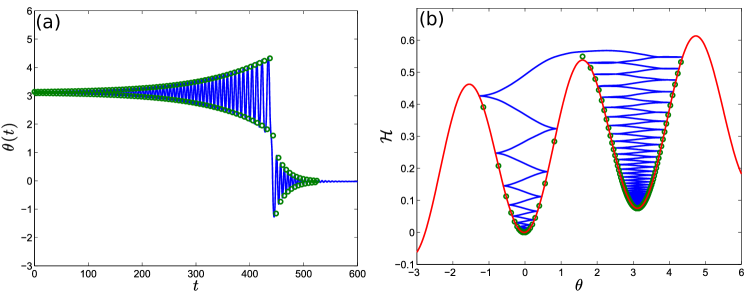
Figure 2: Switching solution (blue line) and its discrete approximation (green circles). Parameters: $\alpha=0.01$, $\Lambda=0.1$, $p_{\perp}=0.3$, $\sigma=0.08$. Panel (a) shows the solution $\theta(t)$, and panel (b) shows the trajectory for this solution in the $\mathcal{H}-\theta$ plane. The red line in (b) shows $V(\theta)$.

To distinguish whether a trajectory results in switching or precession, we then perform a single half-period step on the precessional orbit from $\theta_{C}$ to $\theta_{C}-\pi$, and check whether $\mathcal{H}<V(\theta_{C}-\pi)$: if this is the case, the trajectory moves back to the oscillatory orbits around the well close to $\theta=0$, and decreases in energy towards the fixed point near $\theta=0$, representing switching. If however $\mathcal{H}>V(\theta_{C}-\pi)$ after the precessional half-period, the solution will continue to precess.

In Fig. 2 below, we display the result of such an iterated application of the discrete map, for the same parameters as the switching solution given in Fig. 1(c). In Fig. 2(a), the continuous curve represents the solution to (30), and the points are the predicted peaks of the oscillations, from the discrete map (44). Fig. 2(b) shows the energy of the same solution as a function of $\theta$. Again the blue curve gives $\mathcal{H}(t)$ for the ODE solution, the green points are the prediction of the iterated discrete map, and the red curve is $V(\theta)$. The discrete map predicts the switching behavior quite well, only suffering some error near the switching event, when the change of $\mathcal{H}$ is significant on a single period.

IV.2 Modelling precession

Here we apply the discrete map to a precessional solution—one in which the trajectory, once it escapes the potential well near $\pi$, does not get trapped in the next well, and continues to rotate. Fig. 3(a) below displays such a solution $\theta(t)$ and its discrete approximation, and Fig. 3(b) displays the energy of the same solution. Again, the prediction of the discrete map is excellent.

V Transitions in trajectories

In this section we seek to understand the transitions between the trapping, switching, and precessional regimes as the current parameters $\sigma$ and $p_{\perp}$ are varied.

V.1 Escape Transition

Firstly, let us consider the transition from states which are trapped in a single potential well, such as those in Figs. 1(a,b), to states which can escape and either switch or precess. Effectively, the absolute threshold for this transition is for the value of $\mathcal{H}$ to be able to increase for some value $\theta$ close to the minimum of $V(\theta)$ near $\pi$. Thus, we consider the equation of motion (36) for $\mathcal{H}$, and wish to find parameter values such that $\dot{\mathcal{H}}>0$ for some $\theta$ near $\pi$. This requires that

$$\frac{\omega^{2}}{\sqrt{\Lambda}}(\alpha+2\sigma\Lambda\cos\theta)<0.$$ (45)

Assuming that $\omega\neq 0$, we can see that the optimal value of $\theta$ to hope to satisfy this condition is $\theta=\pi$, yielding a theoretical minimum $\sigma=\sigma_{s}$ for the dimensionless current density for motion to be possible, with

$$\sigma_{s}=\frac{\alpha}{2\Lambda}.$$ (46)

This is similar to the critical switching currents derived in previous work Pinna2013 . We then require $\sigma>\sigma_{s}$ for the possibility of switching or precession. Note that this estimate is independent of the value of $p_{\perp}$.

V.2 Switching–Precessing Transition

We now consider the transition from switching to precessional states. This is rather sensitive and there is not in general a sharp transition from switching to precession. It is due to the fact that for certain parameters, the path that the trajectory takes once it escapes the potential well depends on how much energy it has as it does so. In fact, for a fixed $\alpha,\Lambda$, and values of $\sigma>\sigma_{s}$ we can separate the $(\sigma,p_{\perp})$-parameter space into three regions: (i) after escaping the initial well, the trajectory always falls into the next well, and thus switches; (ii) after escaping, the trajectory may either switch or precess depending on its energy as it does so (and thus depending on its initial condition); (iii) after escaping, the trajectory completely passes the next well, and thus begins to precess.

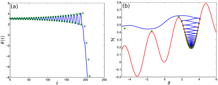
Figure 3: Precessing solution (blue line) and its discrete approximation (green circles). Parameters: $\alpha=0.01$, $\Lambda=0.1$, $p_{\perp}=0.6$, $\sigma=0.1$. Panel (a) shows the solution $\theta(t)$, and panel (b) shows the trajectory for this solution in the $\mathcal{H}-\theta$ plane. The red line in (b) shows $V(\theta)$.

We can determine in which region of the parameter space a given point $(\sigma,p_{\perp})$ lies by studying the discrete map (44) close to the peaks of $V(\theta)$. Assume that the trajectory begins at $\theta(0)=\pi$, and is thus initially in the potential well spanning the interval $\pi/2\leq\theta\leq 3\pi/2$. Denote by $\theta_{C}$ the point close to $\theta=\pi/2$ at which $V(\theta)$ has a local maximum. It is simple to compute

$$\theta_{C}=\frac{\pi}{2}+\frac{1}{2}\sin^{-1}(2\sigma p_{\perp}).$$ (47)

Moreover, it is easy to see that all other local maxima of $V(\theta)$ are given by $\theta=\theta_{C}+k\pi$, for $k\in\mathbb{Z}$.

We now consider trajectories which escape the initial well by crossing $\theta_{C}$. These trajectories have, for some value of the timestep $n$ while still confined in the initial well, an energy value $\mathcal{H}_{n}$ in the range

$$\mathcal{H}_{\text{\scriptsize{trap}}}<\mathcal{H}_{n}<V(\theta_{C}+\pi),$$ (48)

where we define $\mathcal{H}_{\text{\scriptsize{trap}}}$ to be the value of $\mathcal{H}_{n}$ such that the discrete map (44) gives $\mathcal{H}_{n+1}=V(\theta_{C})$. We thus have $\mathcal{H}_{n+1}>V(\theta_{C})$. In order to check whether the trajectory switches or precesses, we then compute $\mathcal{H}_{n+2}$ and compare it to $V(\theta_{C}-\pi)$. We may then classify the trajectories as switching if $\mathcal{H}_{n+2}-V(\theta_{C}-\pi)<0$, and precessional if $\mathcal{H}_{n+2}-V(\theta_{C}-\pi)>0$.

Figure 4 displays a plot of $\mathcal{H}_{n}-V(\theta_{C}+\pi)$ against $\mathcal{H}_{n+2}-V(\theta_{C}-\pi)$. The blue line shows the result of applying the discrete map, while the red line is the identity line. Values of $\mathcal{H}_{n}-V(\theta_{C}+\pi)$ which are inside the range specified in (48) are thus on the negative $x$-axis here. We can classify switching trajectories as those for which the blue line lies below the $x$-axis, and precessing trajectories as those which lie above. In Fig. 4, the parameters are such that both of these trajectory types are possible, depending on the initial value of $\mathcal{H}_{n}$, and thus this set of parameters are in region (ii) of the parameter space. We note that, since the curve of blue points and the identity line intersect for some large enough value of $\mathcal{H}$, this figure implies that if the trajectory has enough energy to begin precessing, then after several precessions the trajectory will converge to one which conserves energy on average over a precessional period (indicated by the arrows). In region (i) of the parameter space, the portion of the blue line for $\mathcal{H}_{n}-V(\theta_{C}+\pi)<0$ would have $\mathcal{H}_{n+2}-V(\theta_{C}-\pi)<0$, while in region (iii), they would all have $\mathcal{H}_{n+2}-V(\theta_{C}-\pi)>0$.

We can classify the parameter regimes for which switching in the opposite direction (i.e. $\theta$ switches from $\pi$ to $2\pi$) is possible in a similar way. It is not possible to have a precessional trajectory moving in this direction ($\dot{\theta}>0$), though.

We may then predict, for a given point $(\sigma,p_{\perp})$ in parameter space, by computing relations similar to that in Fig. 4, which region that point is in, and thus generate a theoretical phase diagram.

In Fig. 5 below, we display the phase diagram in the $(\sigma,p_{\perp})$-parameter space, showing the end results of solving the ODE (30) as a background color, together with predictions of the bounding curves of the three regions of the space, made using the procedure described above. The predictions of the discrete map, while not perfect, are quite good, and provide useful estimates on the different regions of parameter space. In particular, we note that the region where downhill switching reliably occurs (the portion of region (i) above the dashed black line) is estimated quite well. We would also note that we would expect the predictions of the discrete map to improve if the values of $\Lambda$ and $\alpha$ were decreased.

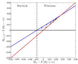
Figure 4: Precession vs switching prediction from the discrete map. Parameters: $\alpha=0.01$, $\Lambda=0.1$, $p_{\perp}=0.35$, $\sigma=0.08$. Values of $\mathcal{H}_{n}-V(\theta_{C}+\pi)$ to the left of the dashed line switch after the next period, the trajectory becoming trapped in the well around $\theta=0$. Values to the right begin to precess, and converge to a precessional fixed point of the discrete map.

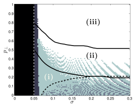
Figure 5: Macrospin solution phase diagram: $\alpha=0.01,\Lambda=0.1$. The background color indicates the result of solving the ODE (30) with initial condition (31): the dark region to the left of the figure indicates solutions which do not escape their initial potential well, and the vertical dashed white line shows the computed value of the minimum current required to escape, $\sigma_{s}=\alpha/(2\Lambda)$. The black band represents solutions which decay, like in Fig. 1(a), while the dark grey band represents solutions like in Fig. 1(b). In the rest of the figure, the green points indicate switching in the negative direction like in Fig. 1(c), grey indicate switching in the positive direction, and white indicates precession like in Fig. 1(d). The solid black curves are the predictions of boundaries of the regions (as indicated in the figure) by using the discrete map, and the dashed line is the prediction of the boundary below which switching in the positive direction is possible.

VI Discussion

We have derived an underdamped PDE model for magnetization dynamics in thin films subject to perpendicular applied spin-polarized currents, valid in the asymptotic regime of small $\alpha$ and $\Lambda$, corresponding to weak damping and strong penalty for out-of-plane magnetizations. We have examined the predictions of this model applied to the case of an elliptical film under a macrospin approximation by using an orbit-averaging approach. We found that they qualitatively agree quite well with previous simulations using full LLGS dynamics ChavesKent15 .

The benefits of our reduced model are that they should faithfully reproduce the oscillatory nature of the in-plane magnetization dynamics, reducing computational expense compared to full micromagnetic simulations. In particular, in sufficiently small and thin magnetic elements the problem further reduces to a single second-order scalar equation.

The orbit-averaging approach taken here enables the investigation of the transition from switching to precession via a simple discrete dynamical system. The regions in parameter space where either switching or precession are predicted, as well as an intermediate region where the end result depends sensitively on initial conditions. It may be possible to further probe this region by including either spatial variations in the magnetization (which, in an earlier study ChavesKent15 were observed to simply ‘slow down’ the dynamics and increase the size of the switching region), or by including thermal noise, which could result in instead a phase diagram predicting switching probabilities at a given temperature, or both.

References

- (1) S. D. Bader and S. S. P. Parkin, Annu. Rev. Condens. Matter Phys. 1, 71 (2010).
- (2) A. Brataas and A. D. Kent and H. Ohno, Nature Mat. 11, 372 (2012).
- (3) A. D. Kent and D. C. Worledge, Nature Nanotechnol. 10, 187 (2015).
- (4) C. J. García-Cervera and W. E, J. Appl. Phys. 90, 370 (2001).
- (5) A. DeSimone, R. V. Kohn, S. Müller and F. Otto Comm. Pure Appl. Math. 55, 1408 (2002).
- (6) R. V. Kohn and V. V. Slastikov, Proc. R. Soc. Lond. Ser. A 461, 143 (2005).
- (7) C. B. Muratov and V. V. Osipov, J. Comput. Phys. 216, 637 (2006).
- (8) A. Capella, C. Melcher and F. Otto, Nonlinearity 20, 2519 (2007).
- (9) A. D. Kent, B. Ozyilmaz and E. del Barco Appl. Phys. Lett. 84, 3897 (2004).
- (10) H. Liu, D. Bedau, D. Backes, J. A. Katine, J. Langer and A. D. Kent Appl. Phys. Lett. 97, 242510 (2010).
- (11) H. Liu, D. Bedau, D. Backes, J. A. Katine, and A. D. Kent, Appl. Phys. Lett. 101, 032403 (2012).
- (12) L. Ye, G. Wolf, D. Pinna, G. D. Chaves-O’Flynn and A. D. Kent, J. Appl. Phys. 117, 193902 (2015).
- (13) K. Newhall and E. Vanden-Eijnden, J. Appl. Phys. 113, 184105 (2013).
- (14) D. Pinna, A. D. Kent and D. L. Stein Phys. Rev. B 88, 104405 (2013).
- (15) D. Pinna, D. L. Stein and A. D. Kent Phys. Rev. B 90, 174405 (2014).
- (16) G. D. Chaves-O’Flynn, G. Wolf, D. Pinna and A. D. Kent, J. Appl. Phys. 117, 17D705 (2015).
- (17) R. V. Kohn and V. V. Slastikov, Arch. Rat. Mech. Anal. 178, 227 (2005).