Input-to-state Stability of Impulsive Systems with Different Jump Maps

Abstract

The paper introduces sufficient conditions for input-to-state stability (ISS) of a class of impulsive systems with jump maps that depend on time. Such systems can naturally represent an interconnection of several impulsive systems with different impulse time sequences. Using a concept of ISS-Lyapunov function for subsystems a small-gain type theorem equipped with a new dwell-time condition to verify ISS of an interconnection has been proven.

1 Introduction

Impulsive systems describe processes that combine continuous and discontinuous behavior. A variety of examples can be found in mathematical modelling of applications in logistics, robotics, population dynamics, etc. A basic mathematical theory of impulsive systems as well as fundamental results on existence and stability of solutions can be found in Samoilenko and Perestyuk (1987) and Lakshmikantham et al. (1989) and references therein.

Nearly at the same time the concept of input-to-state stability (ISS) for systems of ordinary differential equations has been introduced by Sontag (1989). ISS characterizes a behavior of solutions with respect to external inputs. Later it was also studied for discrete-time systems by Jiang and Wang (2001), switched systems by Mancilla-Aguilar and Garcıa (2001) and hybrid systems by Cai and Teel (2005).

ISS properties of impulsive systems were firstly studied by Hespanha et al. (2005). Authors provided a set of Lyapunov-based sufficient conditions for establishing ISS with respect to suitable classes of impulsive time sequences. The same approach was used in Hespanha et al. (2008) to justify integral ISS property of impulsive system.

An important question of ISS theory is establishing sufficient conditions for ISS of interconnected systems. The first results on the ISS property were given for two coupled continuous systems by Jiang et al. (1994) and for an arbitrarily large number ($n\in\mathbb{N}$) of coupled continuous systems by Dashkovskiy et al. (2007). Lyapunov versions of these so-called ISS small-gain theorems were proved by Jiang et al. (1996) (two systems) and by Dashkovskiy et al. (2010) ($n$ systems). Small-gain theorems for impulsive systems with and without time-delay were established by Dashkovskiy et al. (2012). A complementary result for infinite-dimensional impulsive systems were developed by Dashkovskiy and Mironchenko (2013).

The latest developments in the area of interconnections and systems of a large scale were made in a strongly related class of hybrid systems. We refer the reader to papers of Liberzon et al. (2014); Mironchenko et al. (2014); Sanfelice (2014) with the most recent small-gain theorems on ISS of hybrid systems. However, solutions to hybrid systems are defined on hybrid time domains, as opposed to the usual time defined on the real line. As it was mentioned in Hespanha et al. (2008), this leads to a distinct notion of ISS, and some systems that are ISS in impulsive framework are not ISS in the hybrid framework. This motivates an importance of investigation of explicitly impulsive systems apart from hybrid ones.

A significant lack of the previously developed results on interconnections of impulsive systems is that impulsive time sequences of each subsystem must coincide in order to apply known results. The reason for this is trivial: a composition of two impulsive systems with different impulsive time sequences falls out of a class of impulsive systems. Such interconnection requires a jump map to be different depending on time. Moreover, even simple real-processes (for instance in logistics, see Example 1) require for a jump map that varies from time to time.

The aim of this paper is to extend the notion of ISS to impulsive systems with jump maps that depend on time. The novelty of our results is twofold. First, such approach enables modelling of a wider class of processes with continuous and discontinuous dynamics. Second, an interconnection of two impulsive systems will become an impulsive system again. This enables a comprehensive stability analysis of interconnections which subsystems have different impulse time sequences.

The rest of the paper is organized as follows. Section 2 contains a short motivation for the framework extension. An extension of impulsive systems to the case of multiple jump sets is proposed in Section 3. A Lyapunov-like sufficient conditions for ISS of impulsive system along with an appropriate dwell-time condition are presented in Section 4. A small-gain type theorem for a network of two impulsive systems with different impulse time sequences is presented in Section 5. A discussion and a short conclusion complete the paper.

2 Motivation

Well-known ISS results (Hespanha et al. (2008);Dashkovskiy et al. (2012); Dashkovskiy and Mironchenko (2013)) for impulsive systems were developed for a system of the type

$$\begin{array}[]{ll}\begin{cases}\dot{x}(t)=f(x(t),u(t)),\\ x(t)=g(x^{-}(t),u^{-}(t)),\end{cases}&\begin{aligned} t&\not=t_{k},k\in\{1,2,\ldots\},\\ t&=t_{k},k\in\{1,2,\ldots\}\end{aligned}\end{array}$$ (1)

where $\{t_{1},t_{2},t_{3},\ldots\}$ is a strictly increasing sequence of impulse times in $(t_{0},\infty)$ for some initial time $t_{0}$; the state $x(t)\in\mathbb{R}^{N}$ is absolutely continuous between impulses; input $u(t)\in\mathbb{R}^{M}$ is locally bounded and Lebesgue-measurable function; $f$ and $g$ are functions from $\mathbb{R}^{N}\times\mathbb{R}^{M}$ to $\mathbb{R}^{N}$, with $f$ locally Lipschitz. The state $x$ and the input $u$ are assumed to be right-continuous, and to have left limits at all times. We denote by $(\cdot)^{-}$ the left-limit operator, i.e., $x^{-}(t)=\lim_{s\nearrow t}{x(s)}$. However system (1) does not cover a variety of many real processes. Consider the following

2.0.1 Example 1.

Let the number $x\in\mathbb{R}_{\geq 0}$ of goods in a storage be continuously decreasing proportionally to the number of items with rate coefficient $0.2$. But every odd day ($\mathbb{T}_{1}=\{1,3,5,\ldots\}$) a delivery truck doubles the number of items, and every even day ($\mathbb{T}_{2}=\{2,4,6,\ldots\}$) a delivery truck takes out $40\%$ of items. The evolution of this process can be modelled as

$$\begin{array}[]{ll}\begin{cases}\dot{x}(t)=-0.2x(t),\\ x(t)=\begin{cases}2x^{-}(t),\\ 0.6x^{-}(t),\end{cases}\end{cases}&\begin{aligned} t&\not\in\mathbb{T}_{1}\cup\mathbb{T}_{2},\\ t&\in\mathbb{T}_{1},\\ t&\in\mathbb{T}_{2},\end{aligned}\end{array}$$ (2)

System (2) does not fit into the class of systems (1) because its jump map depends on time. Numerical simulations show that a trivial solution to this system is likely to be globally asymptotically stable (see Figure 1).

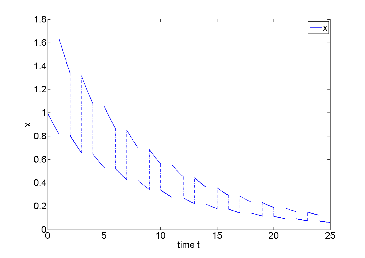
Figure 1: Numerical simulation of solution to system (2) with initial condition $x(0)=1$.

Moreover, if one adds inputs to the right-hand side of the equations the resulting system becomes ISS, however currently there are no theoretical result to verify this. $\square$

Another motivation to consider impulsive systems with jump map that depends on time appears while interconnecting several impulsive systems of a type (1) but with different impulse time sequences. Consider two systems of the type (1) with the states $x_{i}$, inputs $u_{i}$, flow and jump maps $f_{i}$ and $g_{i}$ respectively and impulse time sequences $\mathbb{T}_{i}=\{t^{i}_{1},t^{i}_{2},t^{i}_{3},\ldots\}$, $i=1,2$. Let us interconnect these two systems in the following way

$$u_{1}=h_{2}(u_{2}),\quad u_{2}=h_{1}(u_{1})$$

with some functions $h_{1}$ and $h_{2}$. Then the entire interconnection will have the form

$$\begin{array}[]{ll}\begin{cases}\dot{x}(t)=f(x(t)),\\ x(t)=\begin{cases}\tilde{g}_{1}(x^{-}(t)),\\ \tilde{g}_{2}(x^{-}(t)),\\ \tilde{g}_{3}(x^{-}(t)),\end{cases}\end{cases}&\begin{aligned} t&\not\in\mathbb{T}_{1}\cup\mathbb{T}_{2},\\ t&\in\mathbb{T}_{1},t\not\in\mathbb{T}_{2},\\ t&\not\in\mathbb{T}_{1},t\in\mathbb{T}_{2},\\ t&\in\mathbb{T}_{1},t\in\mathbb{T}_{2},\end{aligned}\end{array}$$ (3)

where $x(t)=(x_{1}(t),x_{2}(t))^{T}$ is the new state, $f(x(t))=\left(f_{1}(x_{1}(t),h_{2}(x_{2}(t))),f_{2}(x_{2}(t),h_{1}(x_{1}(t)))\right)^{T}$ is the flow map and functions

$$\begin{split}\tilde{g}_{1}(x^{-}(t))&=\left(\begin{array}[]{c}g_{1}(x_{1}^{-}(t),h_{2}(x_{2}^{-}(t)))\\ x_{2}^{-}\\ \end{array}\right),\\ \tilde{g}_{2}(x^{-}(t))&=\left(\begin{array}[]{c}x_{1}^{-}\\ g_{2}(x_{2}^{-}(t),h_{1}(x_{1}^{-}(t)))\\ \end{array}\right),\\ \tilde{g}_{3}(x^{-}(t))&=\left(\begin{array}[]{c}g_{1}(x_{1}^{-}(t),h_{2}(x_{2}^{-}(t)))\\ g_{2}(x_{2}^{-}(t),h_{1}(x_{1}^{-}(t)))\\ \end{array}\right)\end{split}$$

define jump maps in different situations (with respect to impulse time sequence). From (3) it is clear that interconnection of two impulsive systems is a system with three different jump maps depending on impulse time sequence. This simple interconnection cannot be written in the form of (1).

In the following sections we will develop sufficient conditions of ISS for systems of types (2), (3). This enables a comprehensive stability analysis of a wide class of processes that combine continuous and discontinuous dynamics as well as their interconnections.

3 Extended Impulsive System

For every $i=1,\ldots,p$, $p\in\mathbb{N}$ let $\mathbb{T}_{i}=\{t^{i}_{1},t^{i}_{2},t^{i}_{3},\ldots\}$ be a strictly increasing sequence of impulse times in $(t_{0},\infty)$ for some initial time $t_{0}$ and

$$\mathbb{T}=\bigcup_{i=1,\ldots,p}{\mathbb{T}_{i}},\quad\bigcap_{i=1,\ldots,p}{\mathbb{T}_{i}}=\emptyset.$$

We consider impulsive system with external inputs

$$\begin{array}[]{ll}\begin{cases}\dot{x}(t)=f(x(t),u(t)),\\ x(t)=g_{i}(x^{-}(t),u^{-}(t)),\end{cases}&\begin{aligned} t&\not\in\mathbb{T},\\ t&\in\mathbb{T}_{i},i=1,\ldots,p,\end{aligned}\end{array}$$ (4)

where the state $x(t)\in\mathbb{R}^{N}$ is absolutely continuous between impulses; input $u(t)\in\mathbb{R}^{M}$ is locally bounded and Lebesgue-measurable function; $f$ and $g_{i},i=1,\ldots,p$ are functions from $\mathbb{R}^{N}\times\mathbb{R}^{M}$ to $\mathbb{R}^{N}$, with $f$ locally Lipschitz. Given a sequence $\mathbb{T}_{i}$, $i=1,\ldots,p$ and a pair of times $s,t$ satisfying $t>s\geq t_{0}$, let $N_{i}(t,s)$ denote the number of impulsive times $t^{i}_{k}\in\mathbb{T}_{i}$ in the semi-open interval $(s,t]$.

As one may see, system (4) coincides with the system (1) when $p=1$. Also, similarly to Samoilenko and Perestyuk (1987) and Lakshmikantham et al. (1989), system (4) allows for jump maps $g_{i}$ to be different for every moment of impulsive jump ($p=\infty$). As it was shown previously, a natural representation of interconnection of two systems of the type (1) requires three sets of impulsive jumps $\mathbb{T}_{1},\mathbb{T}_{2}$ and $\mathbb{T}_{3}$ with the corresponding jump maps $g_{1},g_{2}$ and $g_{3}$ ($p=3$).

To introduce appropriate notion of ISS, we recall the following standard definition: a function $\alpha:[0,\infty)\to[0,\infty)$ is of class $\mathcal{K}$, and we write $\alpha\in\mathcal{K}$, when $\alpha$ is continuous, strictly increasing, and $\alpha(0)=0$. If $\alpha$ is also unbounded, then we say it is of class $\mathcal{K}_{\infty}$, and we write $\alpha\in\mathcal{K}_{\infty}$. A continuous function $\beta:[0,\infty)\times[0,\infty)\to[0,\infty)$ is of class $\mathcal{KL}$, and we write $\beta\in\mathcal{KL}$, when $\beta(\cdot,t)$ is of class $\mathcal{K}$ for each fixed $t\geq 0$, and $\beta(r,t)$ decreases to $0$ as $t\to\infty$ for each fixed $r\geq 0$.

Definition 1

For a given set of time sequences $\mathbb{T}_{i}$, $i=1,\ldots,p$ of impulse times we call system (4) input-to-state stable (ISS) if there exist functions $\beta\in\mathcal{KL}$ and $\gamma\in\mathcal{K}_{\infty}$, such that for every initial condition and every input $u$, the corresponding solution to (4) exists globally and satisfies

$$\begin{split}|x(t)|\leq\max\{\beta(|x(t_{0})|,t-t_{0}),\gamma(\left\|u\right\|_{[t_{0},t]})\}\quad\forall t\geq t_{0},\end{split}$$

where $\left\|\cdot\right\|_{J}$ denotes the supremum norm on an interval $J$.

Definition 2

System (4) is called uniformly ISS over a given set $\mathcal{S}$ of admissible sequences of impulse times if it is ISS for every sequence in $\mathcal{S}$, with $\beta$ and $\gamma$ independent of the choice of the sequence from the class $\mathcal{S}$.

4 Sufficient Conditions for ISS

For analysis of ISS of impulsive systems we adopt the concept of a candidate exponential ISS-Lyapunov function from Hespanha et al. (2008) and state it in the implication form.

Definition 3

Function $V:\mathbb{R}^{n}\to\mathbb{R}$ is called a candidate exponential ISS-Lyapunov function for (4) with rate coefficients $c,d_{1},d_{2},\ldots,d_{p}\in\mathbb{R}$ if $V$ is locally Lipschitz, positive definite, radially unbounded, and whenever $V(x)\geq\gamma(|u|)$ holds it follows that

$$\nabla V(x)\cdot f(x,u) \leq-cV(x)\qquad\forall x\text{~{}a.e.},\forall u,$$ (5)

$$V(g_{i}(x,u)) \leq e^{-d_{i}}V(x)\quad\mbox{~{}}\forall x,u,i=1,\ldots,p$$ (6)

for some function $\gamma\in\mathcal{K}_{\infty}$. In (5), ”$\forall x\text{~{}a.e.}$” should be interpreted as ”for every $x\in\mathbb{R}^{n}$ except, possibly, on a set of zero Lebesgue-measure in $\mathbb{R}^{n}$”.

Theorem 1 (Uniform ISS)

Let $V$ be a candidate exponential ISS-Lyapunov function for (4) with rate coefficients $c,d_{1},\ldots,d_{p}\in\mathbb{R}$ with $d_{i}\not=0$, $i=1,\ldots,p$. For arbitrary constants $\mu,\lambda>0$, let $\mathcal{S}[\mu,\lambda]$ denote the class of impulse time sequences satisfying

$$-\sum_{i=1}^{p}{d_{i}N_{i}(t,s)}-(c-\lambda)(t-s)\leq\mu\quad\forall t\geq s\geq t_{0}.$$ (7)

Then the system (4) is uniformly ISS over $\mathcal{S}[\mu,\lambda]$.

The technique of the proof is based on the proof of Theorems 3.3 and 3.7 from Dashkovskiy et al. (2012). The difference is that by iteration over $N(t_{0},t)$ impulses on interval $(t_{0},t]$ we obtain $\sum_{i=1}^{p}{d_{i}N_{i}(t_{0},t)}$ instead of $dN(t_{0},t)$.

Remark 4.1

In the case of a distinct jump map for every moment of impulsive jumps (the case of $p=\infty$), dwell-time condition (7) can be presented in the form

$$-\sum_{t_{1}^{i}\in(s,t]}{d_{i}}-(c-\lambda)(t-s)\leq\mu\quad\forall t\geq s\geq t_{0}.$$

4.0.1 Example 1 (revisited).

Consider system with external input

$$\begin{array}[]{ll}\begin{cases}\dot{x}(t)=-0.2x(t)+u(t),\\ x(t)=\begin{cases}2x^{-}(t)+u^{-}(t),\\ 0.6x^{-}(t)+u^{-}(t),\end{cases}\end{cases}&\begin{aligned} t&\not\in\mathbb{T}_{1}\cup\mathbb{T}_{2},\\ t&\in\mathbb{T}_{1},\\ t&\in\mathbb{T}_{2}\end{aligned}\end{array}$$ (8)

with $\mathbb{T}_{1}=\{1,3,5,\ldots\}$ and $\mathbb{T}_{2}=\{2,4,6,\ldots\}$. System (8) possesses candidate exponential ISS-Lyapunov function $V=|x|$ with $c=0.2$, $d_{1}=-\ln{2}$ and $d_{2}=-\ln{0.6}$. It satisfies the dwell-time condition (7) with, for instance, $\mu=-d_{1}=\ln{2}$ and $\lambda=0.1$. So system (8) is ISS. Moreover, it means that system with zero input (2) is globally asymptotically stable. $\square$

The dwell-time condition (7) firstly appears in this paper. It generalises the corresponding dwell-time condition from Hespanha et al. (2008) for the case of multiple jump maps. ISS property of system (8) cannot be verified using previously known results. Using the framework of measure differential equations with discontinuous inputs, a similar sufficient condition for asymptotic stability in terms of vectors fields were derived in Tanwani et al. (2015).

5 Interconnected impulsive systems

Let two strictly increasing sequences of impulse times $\widehat{\mathbb{T}}_{i}=\{t^{i}_{1},t^{i}_{2},t^{i}_{3},\ldots\}$, $i=1,2$ be given and $\mathbb{T}:=\widehat{\mathbb{T}}_{1}\cup\widehat{\mathbb{T}}_{2}$. We consider an interconnection of two impulsive systems with inputs of the form

$$\begin{array}[]{ll}\begin{cases}\dot{x}_{i}(t)=f_{i}(x_{1}(t),x_{2}(t),u_{i}(t)),\\ x_{i}(t)=\hat{g}_{i}(x_{1}^{-}(t),x_{2}^{-}(t),u_{i}^{-}(t)),\end{cases}\begin{aligned} t&\not\in\mathbb{T},\\ t&\in\widehat{\mathbb{T}}_{i},\end{aligned}\end{array}$$ (9)

$i=1,2$, where the state $x_{i}(t)\in\mathbb{R}^{N_{i}}$ of the $i$th subsystem is absolutely continuous between impulses; $u_{i}(t)\in\mathbb{R}^{M_{i}}$ is a locally bounded Lebesgue-measurable input, and $x_{j}(t)\in\mathbb{R}^{N_{j}}$, $j\not=i$ can be interpreted as internal inputs of the $i$th subsystem. Furthermore, $f_{i}:\mathbb{R}^{N_{1}}\times\mathbb{R}^{N_{2}}\times\mathbb{R}^{M_{i}}\to\mathbb{R}^{N_{i}}$ and $\hat{g}_{i}:\mathbb{R}^{N_{1}}\times\mathbb{R}^{N_{2}}\times\mathbb{R}^{M_{i}}\to\mathbb{R}^{N_{i}}$, and we assume that the $f_{i}$ are locally Lipschitz for $i=1,2$. All signals ($x_{1},x_{2},u_{1},u_{2}$) are assumed to be right continuous and to have left limits at all times.

We define $N:=N_{1}+N_{2}$, $M:=M_{1}+M_{2}$, $x:=(x_{1},x_{2})^{T}$, $u:=(u_{1},u_{2})^{T}$, $f:=(f_{1},f_{2})^{T}$, and

$$\begin{array}[]{ll}g(x,u)=\begin{cases}g_{1}(x,u):=(\hat{g}_{1}(x,u_{1}),x_{2})^{T},\\ g_{2}(x,u):=(x_{1},\hat{g}_{2}(x,u_{2}))^{T},\\ g_{3}(x,u):=(\hat{g}_{1}(x,u_{1}),\hat{g}_{2}(x,u_{2}))^{T},\end{cases}&\begin{aligned} t&\in\mathbb{T}_{1},\\ t&\in\mathbb{T}_{2},\\ t&\in\mathbb{T}_{3}\end{aligned}\end{array}$$

such that the interconnected system (9) is of the form (4) with $p=3$, $\mathbb{T}_{1}:=\widehat{\mathbb{T}}_{1}\setminus\widehat{\mathbb{T}}_{2}$, $\mathbb{T}_{2}:=\widehat{\mathbb{T}}_{2}\setminus\widehat{\mathbb{T}}_{1}$, and $\mathbb{T}_{3}:=\widehat{\mathbb{T}}_{1}\cap\widehat{\mathbb{T}}_{2}$.

To describe stability properties of the system (9) we adopt the definitions of ISS and ISS-Lyapunov function for subsystem from Dashkovskiy et al. (2012).

Definition 5.1

For given time sequences $\mathbb{T}_{1}$ and $\mathbb{T}_{2}$ of impulse times we call the $i$th subsystem of (9) input-to-state stable (ISS) if there exist functions $\beta_{i}\in\mathcal{KL}$ and $\gamma_{ij},\gamma_{i}\in\mathcal{K}_{\infty}\cup\{0\}$, such that for every initial condition $x_{i}(t_{0})$ and every input $u_{i}$, the corresponding solution to (9) exists globally and satisfies for all $t\geq t_{0}$

$$\begin{split}|x_{i}(t)|\leq\max\{&\beta_{i}(|x(t_{0})|,t-t_{0}),\\ &\max_{j,j\not=i}{\gamma_{ij}(\left\|x_{j}\right\|_{[t_{0},t]})},\gamma_{i}(\left\|u\right\|_{[t_{0},t]})\},\end{split}$$

where $i,j=1,2$. Functions $\gamma_{ij}$ are called gains.

Similarly, a Lyapunov function for a system with several inputs is defined as follows. Assume that for each subsystem of the interconnected system (9) there is a given function $V_{i}:\mathbb{R}^{N_{i}}\to\mathbb{R}_{+}$, which is continuous, proper, positive, and locally Lipschitz continuous on $\mathbb{R}^{N_{i}}\setminus\{0\}$.

Definition 5.2

For $i=1,2$, the function $V_{i}$ is called an exponential ISS-Lyapunov function for the $i$th subsystem of (9) with rate coefficients $c_{i},d_{i}\in\mathbb{R}$ if, whenever $V_{i}(x_{i})\geq\max\{\max_{j,j\not=i}{\gamma_{ij}(V_{j}(x_{j}))},\gamma_{i}(|u_{i}|)\}$ holds, it follows that

$$\nabla V_{i}(x_{i})\cdot f_{i}(x,u_{i})\leq-c_{i}V_{i}(x_{i})\quad\forall x\text{~{}a.e.},\forall u_{i}$$ (10)

and for all $x$ and $u_{i}$ it holds that

$$V_{i}(\hat{g}_{i}(x,u_{i}))\leq\max\{e^{-\hat{d}_{i}}V_{i}(x_{i}),\max_{j,j\not=i}{\gamma_{ij}(V_{j}(x_{j}))},\gamma_{i}(|u_{i}|)\},$$

where $\gamma_{ij},\gamma_{i}$ are some functions from $\mathcal{K}_{\infty}$.

In general, even if all subsystems of (9) are ISS, the whole system may be not ISS. Moreover, since the moments of impulse jumps of each subsystem differ we are unable to employ known small-gain type theorems from Dashkovskiy et al. (2012) and Dashkovskiy and Mironchenko (2013). These theorems consider only one constant $d$ that characterizes the influence of impulses for a given Lyapunov function. In our settings we have a distinct constant for each jump map. The only case to use previously developed results is to majorize system and consider the worst case approach assuming that the state of every subsystem updates at the moments of impulse jumps. This leads to $d:=\min_{i=1,\ldots,p}{\hat{d}_{i}}$. However, such approach is too rough, which means that the ISS of interconnected system may not be verified, although the system possesses ISS property. In the following we prove less conservative Theorem 2. However this theorem also has a limited field of use. It will be discussed in more details in Section 6.

In this paper, to simplify relations and readability, we are concerned with an interconnection of impulsive systems that have exponential ISS-Lyapunov functions $V_{i}$ with linear gains $\gamma_{ij}(r):=\gamma_{ij}\cdot r$, $\gamma_{ij},r>0$. However the proposed results can be extended to the case of non-exponential Lyapunov functions with nonlinear gains.

Theorem 2

Assume that each subsystem of (9) has an exponential ISS-Lyapunov function $V_{i}$, $i=1,2$ with corresponding linear gains $\gamma_{12}$ and $\gamma_{21}$ and rate coefficients $c_{1},c_{2},\hat{d}_{1}\not=0,\hat{d}_{2}\not=0$. Let (9) be written as (4). If

$$\gamma_{12}\cdot\gamma_{21}<1,$$ (11)

then there exists a constant $s_{1}>0$ such that the candidate exponential ISS-Lyapunov function for the whole system (4) can be chosen as

$$V(x):=\max\left\{\frac{1}{s_{1}}V_{1}(x_{1}),V_{2}(x_{2})\right\}.$$ (12)

Its gain is given by

$$\gamma(r):=\max\left\{e^{d_{1}},e^{d_{2}},e^{d_{3}},1\right\}\max\left\{\frac{1}{s_{1}}\gamma_{1}(r),\gamma_{2}(r)\right\},$$

and the rate coefficients are $c:=\min\{c_{1},c_{2}\}$, $d_{1}:=\min\{\hat{d}_{1},-\ln{\frac{1}{s_{1}}\gamma_{12}},-\varepsilon\}$, $d_{2}:=\min\{\hat{d}_{2},-\ln{\gamma_{21}},-\varepsilon\}$, and $d_{3}:=\min\{\hat{d}_{1},\hat{d}_{2},-\ln{\frac{1}{s_{1}}\gamma_{12}},-\ln{\gamma_{21}}\}$, where $\varepsilon>0$ is an arbitrary small constant. In particular, for all $\mu,\lambda>0$ such that the dwell-time condition (7) holds, system (4) is uniformly ISS over $\mathcal{S}[\mu,\lambda]$.

Since small-gain condition (11) is satisfied, it follows from Jiang et al. (1996) that there exists a constant $\sigma>0$ such that $\gamma_{12}<\sigma<\gamma_{21}^{-1}$. Let us define $V$ as in (12) with $s_{1}:=\frac{1}{\sigma}$ and show that this function is a candidate exponential ISS-Lyapunov function for system (4). It can be easily checked that this function is locally Lipschitz, positive definite, and radially unbounded.

Consider open domains $M_{1},M_{2}\subset\mathbb{R}^{N}\setminus\{0\}$ defined by

$$\begin{split}M_{1}:=\left\{(x_{1},x_{2})^{T}\in\mathbb{R}^{N}\setminus\{0\}:\frac{1}{s_{1}}V_{1}(x_{1})>V_{2}(x_{2})\right\},\\ M_{2}:=\left\{(x_{1},x_{2})^{T}\in\mathbb{R}^{N}\setminus\{0\}:V_{2}(x_{2})>\frac{1}{s_{1}}V_{1}(x_{1})\right\}.\end{split}$$

Take an arbitrary $\hat{x}=(\hat{x}_{1},\hat{x}_{2})^{T}\in M_{1}$. It follows that there exists a neighborhood $U$ of $\hat{x}$ such that $V(x)=\frac{1}{s_{1}}V_{1}(x_{1})$ is differentiable for almost all $x\in U$. We define $\bar{\gamma}_{1}(r):=\frac{1}{s_{1}}\gamma_{1}(r)$, $r>0$, and assume that $V(x)\geq\bar{\gamma}_{1}(|u|)$. From the small-gain condition (11) it follows that

$$\begin{split}V_{1}(x_{1})=s_{1}V(x)&\geq\max\{\gamma_{12}V(x),s_{1}\bar{\gamma}_{1}(|u|)\}\\ &\geq\max\{\gamma_{12}V_{2}(x_{2}),\gamma_{1}(|u_{1}|)\}.\end{split}$$

Then, from (10), we obtain that for almost all $x$

$$\dot{V}(x)=\frac{1}{s_{1}}\nabla V_{1}(x_{1})\cdot f_{1}(x,u_{1})\leq-\frac{1}{s_{1}}c_{1}V_{1}(x_{1})=-c_{1}V(x).$$

Now take an arbitrary $\hat{x}\in M_{2}$. Analogously, there exists a neighborhood $U$ of $\hat{x}$ such that $V(x)=V_{2}(x_{2})$ is differentiable for almost all $x\in U$. Assume that $V(x)\geq\gamma_{2}(|u|)$. From the small-gain condition it follows that

$$\begin{split}V_{2}(x_{2})=V(x)&\geq\max\{\gamma_{21}s_{1}V(x),\gamma_{2}(|u|)\}\\ &\geq\max\{\gamma_{21}V_{1}(x_{1}),\gamma_{2}(|u_{2}|)\}.\end{split}$$

Then, from (10), we obtain that for almost all $x$

$$\dot{V}(x)=\nabla V_{2}(x_{2})\cdot f_{2}(x,u_{2})\leq-c_{2}V_{2}(x_{2})=-c_{2}V(x).$$

We have shown that for $c=\min\{c_{1},c_{2}\}$ the function $V$ satisfies (5) with $\bar{\gamma}(r)=\max\{\frac{1}{s_{1}}\gamma_{1}(r),\gamma_{2}(r)\}$, $r>0$ for all $\hat{x}\in M_{1}\cup M_{2}$.

To treat the points $\hat{x}\in\mathbb{R}^{N}\setminus\{M_{1}\cup M_{2}\}$ we need to consider three different cases corresponding to the jump maps $g_{1}$, $g_{2}$, and $g_{3}$:

$$\begin{split}&V(g_{1}(x,u))=V\left(\begin{pmatrix}\hat{g}_{1}(x,u_{1})\\ x_{2}\end{pmatrix}\right)\\ &=\max\left\{\frac{1}{s_{1}}V_{1}(\hat{g}_{1}(x,u_{1})),V_{2}(x_{2})\right\}\\ &\leq\max\left\{\frac{1}{s_{1}}\max\{e^{-\hat{d}_{1}}V_{1}(x_{1}),\gamma_{12}V_{2}(x_{2}),\gamma_{1}(|u_{1}|)\},V_{2}(x_{2})\right\}\\ &\leq\max\left\{\frac{1}{s_{1}}\max\{e^{-\hat{d}_{1}}s_{1}V(x),\gamma_{12}V(x),\gamma_{1}(|u_{1}|)\},V(x)\right\}\\ &\leq\max\left\{e^{-\hat{d}_{1}}V(x),e^{\ln{\frac{1}{s_{1}}\gamma_{12}}}V(x),e^{0}V(x),\frac{1}{s_{1}}\gamma_{1}(|u_{1}|)\right\}\\ &\leq\max\{e^{-d_{1}}V(x),\bar{\gamma}_{1}(|u|)\},\end{split}$$

where $d_{1}:=\min\{\hat{d}_{1},-\ln{\frac{1}{s_{1}}\gamma_{12}},-\varepsilon\}$ with an arbitrary small constant $\varepsilon>0$.

Define $\tilde{\gamma}_{1}(r):=e^{d_{1}}\bar{\gamma}_{1}(r)$. If it holds that $V(x)\geq\tilde{\gamma}_{1}(r)$, it follows that

$$\begin{split}V(g_{1}(x,u))&\leq\max\{e^{d_{1}}V(x),\bar{\gamma}_{1}(|u|)\}\\ &=\max\{e^{d_{1}}V(x),e^{d_{1}}\tilde{\gamma}_{1}(|u|)\}\leq e^{d_{1}}V(x)\end{split}$$

for all $x$ and $u$, and $V$ satisfies (6) with $d_{1}$ and $\tilde{\gamma}_{1}$.

Now consider $V(g_{2}(x,u))$. In the analogues way one can prove that if it holds that $V(x)\geq\tilde{\gamma}_{2}(|u|)$, it follows that

$$V(g_{2}(x,u))\leq e^{d_{2}}V(x)$$

for all $x$ and $u$, and $V$ satisfies (6) with $d_{2}:=\min\{\hat{d}_{2},-\ln{\gamma_{21}},-\varepsilon\}$ and $\tilde{\gamma}_{2}(r):=e^{d_{2}}\gamma_{2}(r)$.

Finally, if it holds that $V(x)\geq\tilde{\gamma}_{3}(|u|)$, it follows that

$$V(g_{3}(x,u))\leq e^{d_{3}}V(x),$$

for all $x$ and $u$, and $V$ satisfies (6) with

$$d_{3}:=\min\left\{\hat{d}_{1},\hat{d}_{2},-\ln{\frac{1}{s_{1}}\gamma_{12}},-\ln{\gamma_{21}}\right\}$$

and $\tilde{\gamma}_{3}(r):=e^{d_{3}}\max\{\bar{\gamma}(r),\gamma_{2}(r)\}$.

Define $\gamma(r):=\max\left\{e^{d_{1}},e^{d_{2}},e^{d_{3}},1\right\}\max\left\{\frac{1}{s_{1}}\gamma_{1}(r),\gamma_{2}(r)\right\}$. Then we conclude that $V$ is a candidate exponential ISS-Lyapunov function with rate coefficients $c,d_{1},d_{2},d_{3}$ and gain $\gamma$. Hence, from Theorem 1 it follows that system (9) is uniformly ISS over $\mathcal{S}[\mu,\lambda]$ if the dwell-time condition (7) holds.

Note that if system (9) does not posses external inputs $u_{i}$, $i=1,2$ then Theorem 2 provides sufficient conditions for global asymptotic stability.

5.0.1 Example 2.

Consider the interconnection of two impulsive systems

$$\begin{cases}&\begin{aligned} \dot{x}(t)&=-(1+\delta)x(1+e^{(1+\delta)|x|})+|y|e^{|y|}\\ \dot{y}(t)&=-y(1+e^{|y|})+|x|e^{|x|}\end{aligned},\mbox{~{}}t\not=k,\\ &x(t)=3x^{-}(t),\hfill\quad\qquad\qquad\qquad\qquad\qquad t=2k-1,\\ &y(t)=2y^{-}(t),\quad\qquad\qquad\qquad\qquad\qquad t=2k\end{cases}$$ (13)

where $k\in\mathbb{N}$, $\delta>0$, the state $(x,y)\in\mathbb{R}\times\mathbb{R}$. Consider functions $V_{1}(x)=|x|$ and $V_{2}(y)=|y|$. Then

$$\begin{split}\dot{V}_{1}(x)&=\operatorname{\mathtt{sign}}{x}\left(-(1+\delta)x\left(1+e^{(1+\delta)|x|}\right)+|y|e^{|y|}\right)\\ &\leq-(1+\delta)|x|\left(1+e^{(1+\delta)|x|}\right)+|y|e^{|y|}\\ &\leq-(1+\delta)V_{1}(x)\left(1+e^{(1+\delta)V_{1}(x)}\right)+V_{2}(y)e^{V_{2}(y)}\\ &\leq-(1+\delta)V_{1}(x)\end{split}$$

if only

$$-(1+\delta)V_{1}(x)e^{(1+\delta)V_{1}(x)}+V_{2}(y)e^{V_{2}(y)}\leq 0.$$ (14)

Consider function $\xi(s)=se^{s}\in\mathcal{K}_{\infty}$. Since for any constant $\alpha\in\mathbb{R}_{+}$: $\xi(\alpha s)=\alpha se^{\alpha s}$ from (14) we get

$$\xi\left((1+\delta)V_{1}(x)\right)\geq\xi\left(V_{2}(y)\right).$$

Since $\xi\in\mathcal{K}_{\infty}$ $\dot{V}_{1}(x)\leq-(1+\delta)V_{1}(x)$ if $V_{1}(x)\geq\frac{1}{1+\delta}V_{2}(y)$. We have proven that for the first subsystem there exists an exponential ISS-Lyapunov function with rate coefficient $c_{1}=1+\delta$ and linear gain function with coefficient $\gamma_{12}=\frac{1}{1+\delta}$. Similarly, one can show that $V_{2}(y)=|y|$ is an exponential ISS-Lyapunov function for the second subsystem with rate coefficient $c_{2}=1$ and linear gain function with coefficient $\gamma_{21}=1$. It is obvious that the small-gain condition $\gamma_{12}\gamma_{21}=\frac{1}{1+\delta}<1$ holds. Hence the continuous part of system (13) has an ISS dynamics and the corresponding candidate exponential ISS-Lyapunov function has the rate coefficient $c:=\min\{c_{1},c_{2}\}=1$. For the discrete part, the corresponding rate coefficients of the exponential ISS-Lyapunov functions for subsystems are $\hat{d}_{1}=-\ln{3}<0$ and $\hat{d}_{2}=-\ln{2}<0$. So the discrete dynamics play against stability of the network. Constant $s_{1}$ from (12) can be chosen in such a way that the rate coefficients of the candidate exponential ISS-Lyapunov function for the entire interconnection are $d_{1}:=\hat{d}_{1}=-\ln{3}$ and $d_{2}:=\hat{d}_{2}=-\ln{2}$. Since the moments of impulsive perturbations do not coincide, from Theorem  2 system (13) is GAS if there exist constants $\mu,\lambda>0$ such that the dwell-time condition

$$\ln{3}N_{1}(t,s)+\ln{2}N_{2}(t,s)-(1-\lambda)(t-s)\leq\mu$$ (15)

holds for all $t\geq s\ \geq t_{0}$. It is easy to verify that there exists a sufficiently small constant $\lambda>0$ such that the dwell-time condition (15) holds for $\mu=\ln{3}$. So system (13) is GAS. $\square$

Note that previously known theorems are not applicable to the system (13). There is the only possibility to majorize system (13) assuming $y(t)=3y^{-}(t)$, so the jump maps of subsystems coincide. Let us denote this system by (13’) and show that this approach is unsuccessful for verifying GAS. From Dashkovskiy et al. (2012), the majorant system (13’) is GAS if

$$\ln{3}\left(N_{1}(t,s)+N_{2}(t,s)\right)-(1-\lambda)(t-s)\leq\mu$$ (16)

holds for some $\mu,\lambda>0$. However even for an arbitrary small $\lambda>0$ there does not exist $\mu$ to satisfy (16) for all $t\geq s\ \geq t_{0}$. Consider semi-open intervals $(s,t]:=(k,k+2i]$, $i\in\mathbb{N}$ and the corresponding sequence of $\mu_{i}$-th that satisfy (16):

$$\mu_{i}\geq\ln{3}+2i\ln{3}-2i(1-\lambda)=\ln{3}+2i\left(\ln{3}-1+\lambda\right).$$

Since for any $\lambda>0$ the expression $\ln{3}-1+\lambda$ is positive, the sequence $\{\mu_{i}\}$ is strictly increasing and unbounded. So (16) does not hold and we cannot verify GAS of the majorant system (13’) and consequently of the original system (13).

6 Discussion and Conclusion

Theorem 2 firstly proposes a small-gain type approach for stability analysis of interconnection of two impulsive systems with different impulse time sequences. A previously known theorems (Dashkovskiy et al. (2012); Dashkovskiy and Mironchenko (2013)) cannot be directly applied to such interconnection. In some cases a majorizing system with more frequent impulsive jumps of the state of each subsystem can be constructed. Additionally, these jumps should be of the worst nature towards stability: the resulting rate coefficient of the corresponding candidate exponential ISS-Lyapunov function will be estimated as $d\leq\min_{i=1,\ldots,p}{\hat{d}_{i}}$. This leads to an excessive conservativeness of the resulting conditions.

In this paper we have developed a more flexible tool for the study of such systems. It is worth to mention that in the case of two different time sequences, the resulting rate coefficient $d_{1}$ does not depend explicitly on $\hat{d}_{2}$ and $d_{2}$ does not depend explicitly on $\hat{d}_{1}$. In some particular cases, new theorem provides fairly accurate sufficient conditions for ISS of the interconnection. It is the case of ISS continuous dynamics ($c_{1},c_{2}>0$) and ”bad” discrete ones ($\hat{d}_{1},\hat{d}_{2}<0$). We would like also to mention that if the times of impulse jumps of subsystems coincide, Theorem 2 reduces to the previously known propositions.

The main weakness of Theorem 2 is that it ignores a positive contribution of impulsive jumps towards ISS of the system. For example, let $\hat{d}_{1}>0$. In the case of $t\in\mathbb{T}_{1}\setminus\mathbb{T}_{2}$ the second part of the state remains unchanged since it is updated according to the rule $x_{2}(t)=x_{2}^{-}(t)$. Using the worst-case approach, it leads to a conclusion that this impulse does not contribute to stability. That is why the conditions of the Theorem 2 for the case of $d_{i}$-s of different signs are more conservative, but it is still valid. Theorem 4.2 from Dashkovskiy et al. (2012) and Theorem 4 from Mironchenko et al. (2014) face a similar problem even to a greater extent since the resulting rate coefficient $d\leq\min_{i=1,\ldots,p}{\hat{d}_{i}}$ in theirs setting. It means that even a single jump map with ”bad” dynamics ($\hat{d}_{i}<0$) leads to the ignorance of positive contribution of all other jump maps.

The ignorance of contribution of ”good” impulses ($\hat{d}_{1},\hat{d}_{2}>0$) makes Theorem 2 inapplicable to study the case of unstable continuous dynamics of some subsystem ($c_{i}<0$) in most cases (excluding completely ”good” discrete dynamics ($\hat{d}_{1},\hat{d}_{2}>0$) and coincidence of impulsive jumps of subsystems), due to inability to satisfy dwell-time condition (7). One of the potential way to overcome this limitation is to construct a new exponential ISS-Lyapunov function for the subsystems with new rate coefficients $\tilde{c}_{i},\tilde{d}_{i}$ such that $\tilde{c}_{i}>0$ for all $i$ as it is suggested in Mironchenko et al. (2014). However such approach leads to substantial increase of internal gains. It is out of the scope of current paper, but it is a good way to prolong this research.

The question of how to account and estimate different types of influences caused by different parts of system in a flexible and precise manner still remains open.

This work was supported by the German Federal Ministry of Education and Research (BMBF) as a part of the research project ”LadeRamProdukt”.

References

- Cai and Teel (2005) Cai, C. and Teel, A.R. (2005). Results on input-to-state stability for hybrid systems. In Proceedings of the 44th IEEE Conference on Decision and Control and 2005 European Control Conference (CDC-ECC’05), 5403–5408.
- Dashkovskiy et al. (2012) Dashkovskiy, S., Kosmykov, M., Mironchenko, A., and Naujok, L. (2012). Stability of interconnected impulsive systems with and without time delays, using Lyapunov methods. Nonlinear Analysis: Hybrid Systems, 6(3), 899–915.
- Dashkovskiy and Mironchenko (2013) Dashkovskiy, S. and Mironchenko, A. (2013). Input-to-state stability of nonlinear impulsive systems. SIAM Journal on Control and Optimization, 51(3), 1962–1987.
- Dashkovskiy et al. (2007) Dashkovskiy, S., Rüffer, B.S., and Wirth, F.R. (2007). An ISS small gain theorem for general networks. Mathematics of Control, Signals, and Systems, 19(2), 93–122.
- Dashkovskiy et al. (2010) Dashkovskiy, S.N., Rüffer, B.S., and Wirth, F.R. (2010). Small gain theorems for large scale systems and construction of ISS Lyapunov functions. SIAM Journal on Control and Optimization, 48(6), 4089–4118.
- Hespanha et al. (2005) Hespanha, J.P., Liberzon, D., and Teel, A.R. (2005). On input-to-state stability of impulsive systems. In Proceedings of the 44th IEEE Conference on Decision and Control and 2005 European Control Conference (CDC-ECC’05), 3992–3997.
- Hespanha et al. (2008) Hespanha, J.P., Liberzon, D., and Teel, A.R. (2008). Lyapunov conditions for input-to-state stability of impulsive systems. Automatica, 44(11), 2735–2744.
- Jiang et al. (1994) Jiang, Z.P., Teel, A.R., and Praly, L. (1994). Small-gain theorem for ISS systems and applications. Mathematics of Control, Signals and Systems, 7(2), 95–120.
- Jiang et al. (1996) Jiang, Z.P., Mareels, I.M., and Wang, Y. (1996). A Lyapunov formulation of the nonlinear small-gain theorem for interconnected ISS systems. Automatica, 32(8), 1211–1215.
- Jiang and Wang (2001) Jiang, Z.P. and Wang, Y. (2001). Input-to-state stability for discrete-time nonlinear systems. Automatica, 37(6), 857–869.
- Lakshmikantham et al. (1989) Lakshmikantham, V., Bainov, D., and Simeonov, P.S. (1989). Theory of impulsive differential equations. World Scientific.
- Liberzon et al. (2014) Liberzon, D., Nesic, D., and Teel, A.R. (2014). Lyapunov-based small-gain theorems for hybrid systems. IEEE Transactions on Automatic Control, 59(6), 1395–1410.
- Mancilla-Aguilar and Garcıa (2001) Mancilla-Aguilar, J. and Garcıa, R. (2001). On converse Lyapunov theorems for ISS and iISS switched nonlinear systems. Systems & Control Letters, 42(1), 47–53.
- Mironchenko et al. (2014) Mironchenko, A., Yang, G., and Liberzon, D. (2014). Lyapunov small-gain theorems for not necessarily ISS hybrid systems. In Proceedings of the 21th International Symposium on Mathematical Theory of Systems and Networks (MTNS 2014), 1001–1008.
- Samoilenko and Perestyuk (1987) Samoilenko, A. and Perestyuk, N. (1987). Differential equations with impulse effect. Visca Skola, Kiev.
- Sanfelice (2014) Sanfelice, R. (2014). Input-output-to-state stability tools for hybrid systems and their interconnections. IEEE Transactions on Automatic Control, 59(5), 1360–1366.
- Sontag (1989) Sontag, E.D. (1989). Smooth stabilization implies coprime factorization. IEEE Transactions on Automatic Control, 34(4), 435–443.
- Tanwani et al. (2015) Tanwani, A., Brogliato, B., and Prieur, C. (2015). Stability notions for a class of nonlinear systems with measure controls. Mathematics of Control, Signals, and Systems, 27(2), 245–275.