Tracing outflows in the AGN forbidden region with SINFONI

Abstract

Context. AGN driven outflows are invoked in numerical simulations to reproduce several observed properties of local galaxies. The z ¿ 1 epoch is of particular interest as it was during this time that the volume averaged star formation and the accretion rate of black holes were maximum. Radiatively driven outflows are therefore believed to be common during this epoch.

Aims. We aim to trace and characterize outflows in AGN hosts with high mass accretion rates at z ¿ 1 using integral field spectroscopy. We obtain spatially-resolved kinematics of the [O iii] $\lambda$5007 line in two targets which reveal the morphology and spatial extension of the outflows.

Methods. We present J and H+K band SINFONI observations of 5 AGNs at 1.2 ¡ z ¡ 2.2. To maximize the chance of observing radiatively driven outflows, our sample was pre-selected based on peculiar values of the Eddington ratio and the hydrogen column density of the surrounding interstellar medium. We observe high velocity ($\sim$600-1900 km/s) and kiloparsec scale extended ionized outflows in at least 3 of our targets, using [O iii] $\lambda$5007 line kinematics tracing the AGN narrow line region. We estimate the total mass of the outflow, the mass outflow rate, and the kinetic power of the outflows based on theoretical models and report on the uncertainties associated with them.

Results. We find mass outflow rates of $\sim 1-10\leavevmode\nobreak\ M_{\odot}$/yr for the sample presented in this paper. Based on the high star formation rates of the host galaxies, the observed outflow kinetic power and the expected power due to the AGN, we infer that both star formation and AGN radiation could be the dominant source for the outflows. The outflow models suffer from large uncertainties, hence we call for further detailed observations for an accurate determination of the outflow properties to confirm the exact source of these outflows.

1 Introduction

It is a well established fact that most galaxies in the Universe host a super massive black hole (SMBH) in their nucleus (Magorrian et al., 1998; Kormendy et al., 2011). These black holes grow by accretion of surrounding gas and dust (Silk & Rees, 1998) and may turn active for a certain period of time ($\sim$10⁵-10⁷ yrs) (Martini & Weinberg, 2001; Schawinski et al., 2015; King & Nixon, 2015). Various galaxy evolutionary models invoke outflows driven by active galactic nuclei (AGN) to reproduce several properties of local massive galaxies (Silk & Rees, 1998; Granato et al., 2004; Di Matteo et al., 2005; Croton et al., 2006; Hopkins & Beacom, 2006; Menci et al., 2006; Fabian, 2012; King & Pounds, 2015). Such outflows couple to the surrounding gas and dust and this process, named AGN feedback, is invoked to explain various observed properties such as the black hole and bulge mass relation and the exponential break in the galaxy luminosity function, to name a few (Silk & Mamon, 2012; Kormendy & Ho, 2013).

The coupling between the outflows and the interstellar medium (ISM) could be in the form of mechanical energy, commonly called jet-mode feedback or radiation energy, called the radiative-mode feedback (see Fabian 2012 and Heckman & Best 2014 for a recent review). Jet-mode feedback occurs in black holes having low mass accretion rates. The outflows from such black holes are in the form of relativistic jets with narrow opening angles launched along the axis of the accretion disc. The impact of such feedback mode has been confirmed through X-ray observations of the centres of galaxy clusters or groups with a radio-loud AGN in their centres (Cavagnolo et al., 2011; David et al., 2011; Nesvadba et al., 2008, 2011). On the other hand, black holes with high mass accretion rates are more likely to drive the radiative feedback mode since these radiative winds are believed to originate from the accretion disc (Granato et al., 2004; Di Matteo et al., 2005; Menci et al., 2008; Nayakshin, 2014). Although there is some observational evidence for the presence of radiative feedback in a few objects (Cano-Díaz et al., 2012; Zakamska et al., 2016; Cresci et al., 2015; Perna et al., 2015a; Carniani et al., 2015), we are far from reaching a general conclusion on its impact on the host galaxy.

Outflows have been commonly revealed in local as well as high redshift galaxies using X-ray and UV absorption line studies with velocities reaching ¿1000 km/s (Crenshaw et al., 1999; Chartas et al., 2002; Ganguly et al., 2007; Piconcelli et al., 2005; Tombesi et al., 2010). Since the radiative mode of feedback should be more relevant at $1<z<3$, the epoch of peak volume averaged accretion density of the black holes and the star formation density of the galaxies (Shankar et al., 2009; Madau & Dickinson, 2014), there has been an increasing interest to observe galaxies in this redshift range to detect such outflows. In order to quantify their impact on the host galaxy one needs to determine their spatial extension and energetics. Long slit spectroscopy has been widely used to detect such outflows from the presence of broad and extended emission line profiles in the object spectra (Alexander et al., 2010; Harrison et al., 2012; Brusa et al., 2015a). However, one dimensional spectroscopy has the disadvantage that the spatial information and the outflow morphology cannot be inferred from it. Integral field spectroscopy (IFS) is the ideal tool as one can get an idea of both the spatial extension and the morphology of the outflow around the host galaxy in addition to obtaining the total gas content traced by the respective emission lines. In recent years, there has been extensive work on this front using IFS on local as well as high redshift quasars. A few examples of such works are described in brief below.

Harrison et al. (2014) used GMOS-IFU (Gemini Multi Object Spectrograph-Integral Field Unit) observations to spatially resolve ionized gas kinematics in a sample of 16 local radio-quiet luminous Type 2 AGN. They found high velocity and disturbed gas extended over scales of the host galaxies in all of their objects. Though no specific mechanism behind such outflows, i.e. star formation driven or AGN driven, is favored for the sample in general, the most extreme ionized gas velocities seem to be due to the AGN. Husemann et al. (2013) also studied the gas kinematics of a sample of $\sim$30 low redshift QSOs using Potsdam Multi-Aperture Spectrophotometer (PMAS) where the disturbed gas kinematics is attributed to small scale radio-jet and cloud interactions rather than being AGN-driven. Cano-Díaz et al. (2012) found an extended kiloparsec scale quasar driven outflow for a high redshift Type 1 quasar using Spectrograph for INtegral Field in the Near Infrared (SINFONI) data. The outflow was asymmetric in morphology and the star formation, traced by the narrow component of H$\alpha$ line, was mostly found in the regions not directly affected by the strong outflow. This was one of the first direct observational evidence of a negative AGN-feedback. Cresci et al. (2015) also detected an extended outflow for a high redshift Type 2 quasar. However, in this case, the outflow seems to affect the distribution of star formation in the host galaxy such that star formation is suppressed in the regions dominated by ionized outflows, but enhanced at the edges of the outflow, making it one of the first observational evidences of both negative and positive feedback at play in a galaxy. Finally, Carniani et al. (2015) studied a sample of six high redshift luminous quasars and found extended kiloparsec scale and high velocity outflows in all their objects. These studies demonstrate the capability of IFS to investigate the impact of AGN on host galaxies, both at high as well as low redshifts. They also suggest that outflows are very common in this redshift range, which should be ideal to study AGN feedback due to radiation pressure driven outflows.

In most of these works, the key diagnostic feature for the presence of kiloparsec scale outflows is the presence of asymmetric [O iii] $\lambda$5007 profiles. [O iii] $\lambda$4959,5007 are ideal tracers of ionized gas in the narrow line region (NLR) as it could not be emitted from the high density sub-parsec scales of the broad line region (BLR). The direction of the outflow can be inferred from the presence of a blue or a red wing in the asymmetric [O iii] $\lambda$5007 profile, which indicates gas flow towards or away from the observer respectively. Assuming a bi-conical outflow morphology in most galaxies, it is not uncommon to observe only the blue wing as the red wing is thought to be obscured by dust in the host galaxy.

IFS observations, as the ones listed above, are very expensive in terms of telescope time, and therefore previous studies have always tried to pre-select the targets in order to maximize the chances of observing the AGN in an outflowing phase (Lípari & Terlevich, 2006; Brusa et al., 2015a). We have recently completed a SINFONI program at VLT on a sample of five radio quiet Quasi-stellar objects (QSOs) at $1.2<z<2.2$. The main goal of this program was to prove the effectiveness of selecting AGN in an outflowing phase based on the peculiar values of the Eddington ratio (which is the ratio of the bolometric luminosity and the Eddington luminosity) or its mass accretion rate and column density of the surrounding interstellar medium. We selected only radio-quiet QSOs since the main goal was to use this selection criterion for studies on the impact of radiative feedback on the host galaxy.

This paper is arranged as follows: in Sec. 2, we present the selection strategy of our sample, in Sec. 3, we discuss the observations and the technical details of the data reduction procedure, Sec. 4 presents a detailed description of line fitting, creation of kinematic maps and the velocity definitions used in the paper. In Sec. 5, we describe the properties of individual objects derived from the line fitting and the kinematic maps. In Sec. 6, we provide details about the formulas used and the assumptions that go into our model while deriving the outflow properties. In Sec. 7 we discuss our results and compare them with previous work and finally the conclusions are presented in Sec. 8. Throughout this paper, we use an $H_{o}$ = 70 km s^-1, $\Omega_{\Lambda}$ = 0.7 and $\Omega_{M}$ = 0.3 cosmology.

2 Sample selection

As mentioned before, to maximize the chance of observing outflows driven by an AGN, we need to pre-select our objects based on peculiar values of the physical properties of the black hole such as its mass accretion rate or the Eddington ratio and the column density of the surrounding interstellar medium (ISM). Radiatively driven winds are believed to originate from the acceleration of the disk outflows by the AGN radiation field (Begelman, 2003). Therefore, our selection criterion is skewed towards objects showing high mass accretion rates or equivalently objects having higher Eddington ratio. An object at higher Eddington ratio, will have a tendency to induce a larger radiation pressure on the surrounding ISM. The additional constraint on the column density is motivated by the impact of the radiation pressure generated by the SMBH on the cold gas responsible for the nuclear obscuration (Fabian et al., 2008). The ISM might be able to withstand the high radiation pressure from the AGN provided it has enough gravitational support, an estimate of which can be obtained from the hydrogen column density measurements. The coupling area between the radiation pressure and that of the surrounding gas is given by the cross section of the particles and in presence of a gas (say a dominant atom like hydrogen), this would be simply the Thomson cross section. However, the ISM consists of both gas and dust grains and in the presence of dust radiation pressure is more efficient due to its higher cross section, thereby lowering the Eddington limit. The effective Eddington limit due to interaction with dust, defined at the balance between radiation pressure and gravity, can be a factor of 1000 lower than the “classical” $\mathrm{L_{Edd}}$ for a gas with a Galactic dust-to-gas ratio exposed to a typical quasar spectrum. The result is that long lived clouds would avoid a region of intermediate column densities and high Eddington ratios. Fig. 1 shows the possible dividing lines between the objects having long-lived clouds (or in other words, those which are not expected to show outflows) shown by the grey region and those which are expected to be in an active outflowing phase (or the ”forbidden region” for long lived clouds), shown by the un-shaded region labeled as ”Outflows”, adapted from Fabian et al. (2008). The curve labeled ”1” in Fig. 1 shows the effective Eddington limit for a standard dust abundance for a galaxy while the dashed and dotted lines are for dust abundance of 0.3 and 0.1 of galactic dust abundance respectively.

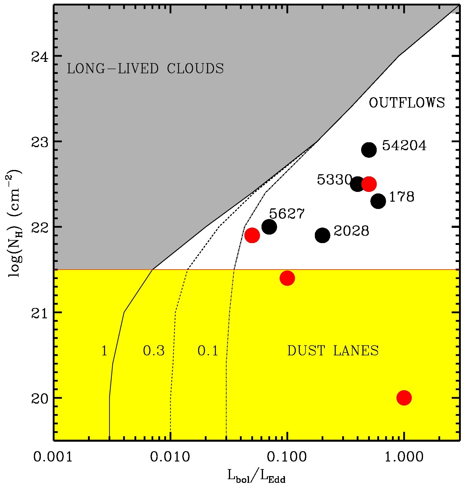
Figure 1: Our sample from the COSMOS field in the hydrogen column density, $\mathrm{N_{H}}$ vs. Eddington ratio, $\lambda$ = $\mathrm{L_{bol}/L_{Edd}}$ plot, adapted from Fabian et al. (2008). The data points from this work are depicted in black circles, while those in red circles have been obtained from Brusa et al. (2015a) for the objects for which the presence of outflows have been verified (see Sec. 7). Various regions of the plot are divided by the expected Eddington limit curves shown in solid, dashed and dotted lines representing galactic dust abundance, 0.3 and 0.1 of the galactic dust abundance respectively. The objects in grey regions are expected to have long lived clouds, while those on the un-shaded region are expected to be in a ”blow-out” or an outflowing phase.

We looked for objects in this forbidden region from the full XMM-COSMOS catalogue (Scoville et al., 2007; Hasinger et al., 2007; Cappelluti et al., 2009) which consists of $\sim$1800 AGN from the entire 2 deg² COSMOS field, with data having a wavelength coverage from radio to UV, with additional information on the morphology, stellar masses, star formation rate and infrared (IR) luminosities of the host galaxies (Brusa et al., 2010; Salvato et al., 2011; Civano et al., 2012; Bongiorno et al., 2012; Rosario et al., 2012). We restrict our study to objects at z¿1 because it is at these redshifts that we expect the radiative feedback to have more significant impact. Our parent sample consisted of 49 objects with z=1.2-2.2, having secure spectroscopic redshifts, black hole mass and bolometric luminosity measurements (to measure the Eddington ratio, $\lambda$ = $\mathrm{L_{bol}/L_{Edd}}$) and reliable column density. The column densities have been derived from detailed X-ray spectral fits (Mainieri et al., 2007; Lanzuisi et al., 2013), the bolometric luminosities have been estimated from SED fitting (Lusso et al., 2011) and the black hole masses from broad MgII lines in the optical spectra (Merloni et al., 2010; Matsuoka et al., 2013) using the virial theorem. Since we want to detect the presence of radiative outflows, we exclude 6 objects which are radio loud with radio-to-optical flux density ratio (R = log($\mathrm{S_{1.4GHz}/S_{V}}$)) $>1.4$. Of the remaining 43 objects which are radio-quiet, 20 are in the forbidden region. Of these, we followed up the five best candidates in terms of the location of the [O iii] $\lambda$4959,5007 emission lines compared to the OH sky emission lines in the infrared spectra. To estimate the stellar mass of the host galaxies, we used an SED fitting technique to model the observed photometry with a galactic and an AGN component (Bonzini et al., 2013). We took advantage of the superb photometry up to the Herschel bands to have a good estimate of the far-infrared (FIR) emission which we used as a tracer of the star-formation (Bonzini et al., 2015). The basic properties of the selected objects are listed in Table 1. The results of the analysis of XID2028, one of the objects from our selection sample, were published in Cresci et al. (2015). In this paper, we will present some of the information from XID2028 data which were not reported in Cresci et al. (2015) and the analysis of the rest of the sample from our selection.

Object ID	RA	DEC	z	log($\mathrm{L_{bol}}$)	log($\mathrm{m_{bh}}$)	log($\mathrm{N_{H}}$)	$\mathrm{M_{acc}}$	$\mathrm{L/L_{edd}}$	Log M*	SFR
	(h:m:s)	∘:′:′′		(erg/s)	($\mathrm{M_{\odot}}$)	(cm-2)	(M⊙/yr)		(M⊙)	(M⊙/yr)
(1)	(2)	(3)	(4)	(5)	(6)	(7)	(8)	(9)	(10)	(11)
178	10 00 14	02 28 37	1.253	45.7	7.78	22.3	0.8	0.6	10.8	134
5330	09 59 30	02 41 26	2.169	45.9	8.22	22.5	1.2	0.4	10.5	101
5627	09 58 44	01 43 09	1.337	45.7	8.77	22.0	0.8	0.07	10.4	157
54204	09 58 20	02 03 02	1.356	46.1	8.27	22.9	1.7	0.5	10.7	438
2028	10 02 11	01 37 07	1.592	46.3	8.83	21.9	2.8	0.2	11.6	250

Table 1: Our sample from the COSMOS field. Column (1): The X-ray ID of the objects; columns (2) and (3): Optical coordinates (J200); Column (4): the spectroscopic redshift of the targets; column (5) Bolometric luminosity from SED fitting; column (6) Black hole mass from broad MgII lines; column (7): column density from X-ray spectral fits; column (8): Mass accretion rate of the black hole; column (9): the Eddington ratio of the black hole; column (10): stellar mass of the host galaxy and column (11): star formation rate of the host galaxy following the procedure by Bonzini et al. 2015. See Sec. 2 for a detailed description of the selection procedure.

Object ID	$\mathrm{\lambda_{narrow}}$	$\mathrm{v_{narrow}}$	$\mathrm{\lambda_{broad}}$	$\mathrm{v_{broad}}$	$\mathrm{\Delta v}$
	($\mu$m)	(km/s)	($\mu$m)	(km/s)	(km/s)
(1)	(2)	(3)	(4)	(5)	(6)
178	1.1310 $\pm$ 0.0001	308 $\pm$ 4	1.1299 $\pm$ 0.0001	1250 $\pm$ 130	-275 $\pm$ 46
5330	1.5930 $\pm$ 0.0001	557 $\pm$ 21	-	-	-
5627	1.1766 $\pm$ 0.0001	206 $\pm$ 66	1.1765 $\pm$ 0.0001	537 $\pm$ 50	-9 $\pm$ 4
54204	1.1810 $\pm$ 0.0002	305 $\pm$ 71	1.1796 $\pm$ 0.0004	1796 $\pm$ 882	-359 $\pm$ 134
2028*	1.2989 $\pm$ 0.0001	366 $\pm$ 3	1.2976 $\pm$ 0.0001	611 $\pm$ 48	-300 $\pm$ 50

Table 2: [O iii] $\lambda$5007 line fitting parameters for the J band integrated spectra of XID178, XID5627, XID54204 and XID2028 and H band spectra of XID5330. Details of the line fitting and the contraints are mentioned in Sec. 4. (1) The X-ray ID of our sample; (2) the central wavelength of the narrow Gaussian component of [O iii] $\lambda$5007 line; (3) the velocity corresponding to the width (FWHM) of the narrow Gaussian component; (4) the central wavelength of the broad Gaussian component of [O iii] $\lambda$5007 line; (5) the velocity corresponding to the width (FWHM) of the broad Gaussian component; (6) velocity offset between the centroids of the narrow and the broad Gaussian components.

3 Observations and data reduction

The aim of our observations is to confirm the presence of outflowing winds in such short-lived objects, and spatially resolve outflows on the scale of the host galaxy i.e. several kpcs. As mentioned before, the key diagnostic feature used to detect outflowing gas is the presence of broad and extended forbidden [O iii] lines at $\lambda$ = 5006.8 $\AA$. This traces the ionized gas in the narrow line region (NLR), which could be extended up to the scale of the host galaxy.

At the redshift of our objects, the [O iii] $\lambda$4959,5007 lines fall in the near-infrared (NIR) and therefore we used SINFONI (Eisenhauer et al., 2003) at the UT4, Very Large Telescope (VLT). Observations were taken between January-March, 2014 as part of the program 092.A-0144 (PI Mainieri). The observations were carried out in seeing limited mode in J band (targets with X-ray ID (XID): XID178, XID5627, XID54204) providing a spectral resolution of 2000 and H+K band (XID5330) providing a spectral resolution of 1500. SINFONI provides rectangular pixels with a spatial scale of 0.125”$\times$0.25”, which is re-sampled to a square pixel with a spatial scale of 0.125”$\times$0.125” and a total field of view (FOV) of 8”$\times$8”. This means that the gas kinematics can be traced to a spatial scale of few tens of kpc for the entire FOV for galaxies at $z>1$. In the observations, the object was dithered by 3.5” across the field of view to ensure an optimal sky subtraction during the data reduction process without losing observing time. The total integration time on source for XID178, XID5627 and XID54204 was about 3.5 hours while for XID5330 it was about 50 minutes reaching depths of 9.67, 2.84, 4.96 and 1.29 $\mathrm{\times 10^{-15}erg\leavevmode\nobreak\ s^{-1}cm^{-2}\mu m^{-1}}$ respectively. The air mass for all the observation blocks was between X$\sim$ 1.1-1.2 for XID178, X$\sim$ 1.1-1.4 for XID5627, X$\sim$ 1.2-1.4 for XID5330 and X$\sim$ 1.7-2.0 for XID54204. The standard stars for telluric and point spread function (PSF) estimation were observed shortly before and after each observing block with an air mass within 0.2 of that of the science observations.

The data were reduced using the ESO-SINFONI pipeline (version 2.5.2) which corrects for bad pixels and distortions, applies a flat field and performs a wavelength calibration. The final image of the object is reconstructed in the form of 32 slices which contains both the spatial and the spectral information. The raw science frames were first corrected for cosmic ray features using the Laplacian Cosmic Ray Identification procedure (L. A. Cosmic) by van Dokkum (2001) before being fed into the pipeline. The sky subtraction was done externally using the improved procedure proposed by Davies (2007). To remove the infrared sky background, adjacent science frames were used as sky for the object. Two consecutive frames are separated by $\sim$10 minutes, a time interval over which the infrared sky should not change significantly. The final science frames were obtained after correcting for telluric features and flux calibrating the cube using the standard star observed before or after each observing blocks. The header information was used to combine different science cubes within the same observing block while the flux calibrated cubes of different observing blocks were combined by measuring the offset in the centroid emission in a given spectral channel.

4 Data analysis

For each of the final science cubes, the integrated spectrum was extracted from a circular region, centred at the object position and with a radius that maximizes the signal-to-noise ratio (S/N) of the [O iii] $\lambda$5007 line. Similar to previous studies (e.g. Harrison et al. 2014; Perna et al. 2015a) we performed a simultaneous fit of the continuum, [O iii] $\lambda$5007 and [O iii] $\lambda$4959 using the IDL routine MPFIT (Markwardt, 2012). The H$\beta$ line remained undetected or it was very faint for all our objects. The errors were estimated from the standard deviation of the spectrum extracted from an object-free region of the SINFONI field of view. Eq. 1 below shows the mathematical form of the function used for line fitting:

$$f(x)=a\cdot e^{-b\cdot x}+\xi_{1}(x)+\xi_{2}(x)$$ (1)

where the first term corresponds to the local continuum with $a$ and $b$ as free parameters. For fitting the overall [O iii] $\lambda$5007 profile, we used either a single or a double Gaussian, the choice of which depended on the S/N of the data and the ability of the components to reproduce the emission line profile. $\xi_{1}$ and $\xi_{2}$ in Eq. 1 correspond to these two Gaussian components - a narrow and a broad component, each with three free parameters defining the central wavelength, width and the flux. The narrow component corresponds to the systemic line which is at rest with respect to the host galaxy, while the broad component(s) would trace the outflowing or the turbulent gas. For all the line profiles, the narrow and broad line widths were constrained. For the narrow Gaussian component, we assume a maximum width (FWHM) of $\sim$500 km/s corresponding to the rotational velocity of the host galaxy and motion in the NLR while the width of the broad Gaussian was kept greater than 500 km/s to decouple it from the narrow component. When only a single Gaussian was used no constrains on the line width were applied. The line fitting was checked by plotting the residuals of the fit over the [O iii] $\lambda$5007 profile. The parameters of [O iii] $\lambda$4959 were coupled to those of [O iii] $\lambda$5007, imposing the same velocity dispersion and a flux ratio of $\mathrm{f_{[{O\textsc{iii}}]5007}/f_{[{O\textsc{iii}}]4959}}\approx$ 3 since they are emitted from the same gas (Storey & Zeippen, 2000; Dimitrijević et al., 2007). The line fit results of the integrated spectrum for each object are given in Table 2 where we list the wavelength ($\mu$m) and width (FWHM in km/s) of the individual Gaussian components and the velocity offset between their centroids.

Since we are interested in spatially resolved kinematics, similar line fitting procedure was performed across the entire field of view for each spaxel separately. The robustness of the fitting procedure across each pixel was checked by creating a residual map of the entire [O iii] $\lambda$5007 profile. From the results of the spaxel by spaxel fit, we constructed flux maps. Wherever necessary, a re-binning was performed on the cube to improve the S/N across each spaxel. Clearly, this increases the spatial scale of each pixel in the field of view.

Wherever possible, for a better quantitative estimate of the spatial extension of the emission, we created maps for the narrow and the broad components of the [O iii] $\lambda$5007 line profile separately, tracing the gas at rest with respect to the system and the outflowing gas. To verify if the emission is extended, we derived the surface brightness profiles of the narrow and the broad components as a function of radius from the peak of the flux weighted mean of the maps. These were compared to the surface brightness profile of the PSF star, which was observed shortly before or after the science observations. We would conclude that the narrow or broad component emission is truly extended if there is an excess in emission of the surface brightness profile compared to the bona-fide point like source represented by the PSF star.

For determining the errors on our measurements, we created 100 mock data cubes by adding Gaussian random noise to the data based on the standard deviation of the spectra extracted from an object free region. The fitting procedure described earlier was repeated for each of these mock cubes (without any constraints on the parameters) and the error associated is the standard deviation of these 100 measurements.

The outflow velocities were estimated from the [O iii] $\lambda$5007 in the integrated spectrum of the objects using different prescriptions adopted previously in the literature. Due to the low S/N in each spaxel despite the re-binning procedure, we did not create velocity maps. We used non-parametric analysis of the line profile and refer the reader to Zakamska & Greene (2014); Liu et al. (2013); Rupke & Veilleux (2013) and Perna et al. (2015a) among others for a detailed description of this procedure. The advantages of using a non-parametric measurement is that it does not depend on the details of the fitting procedure and the properties of the individual Gaussian components in the model. After subtracting the continuum and reproducing the residual line profile, the velocities at different percentiles are evaluated using the cumulative flux function $F(v)=\int_{-\infty}^{v}F_{v}(v^{\prime})dv^{\prime}$, where $F_{v}$ is the line profile in the velocity space. The zero velocity is taken to be at the peak of the line profile, which is the redshifted wavelength of [O iii] $\lambda$5007. The velocity at $x$ percentile, $\mathrm{v_{x}}$ is defined as the velocity at which the cumulative flux function reaches $x$ percent of the overall flux of the asymmetric line profile. Throughout this work, we have calculated $\mathrm{v_{10}}$ and $\mathrm{w_{80}=v_{90}-v_{10}}$ for the entire [O iii] $\lambda$5007 profile on the integrated spectra of the objects i.e. the velocities at the 10th percentile and the width containing 80% of the total flux respectively and $\mathrm{v_{10}}$ on the broad-only Gaussian component as estimates of outflow velocity.

These diagnostics have been used in the literature to estimate the outflow velocities and we will compare these values for our targets to estimate the uncertainties affecting such measurements (see Sec. 7). Finally, in the kinematic analysis, we assume that the highest velocity is reached in the outermost region of the outflow.

5 Results

In the following subsections, we will present the results of the data analysis described above for the individual targets. We refer the reader to Table 2 for the results of line fitting for the integrated spectra of each object.

5.1 XID178 and XID5627

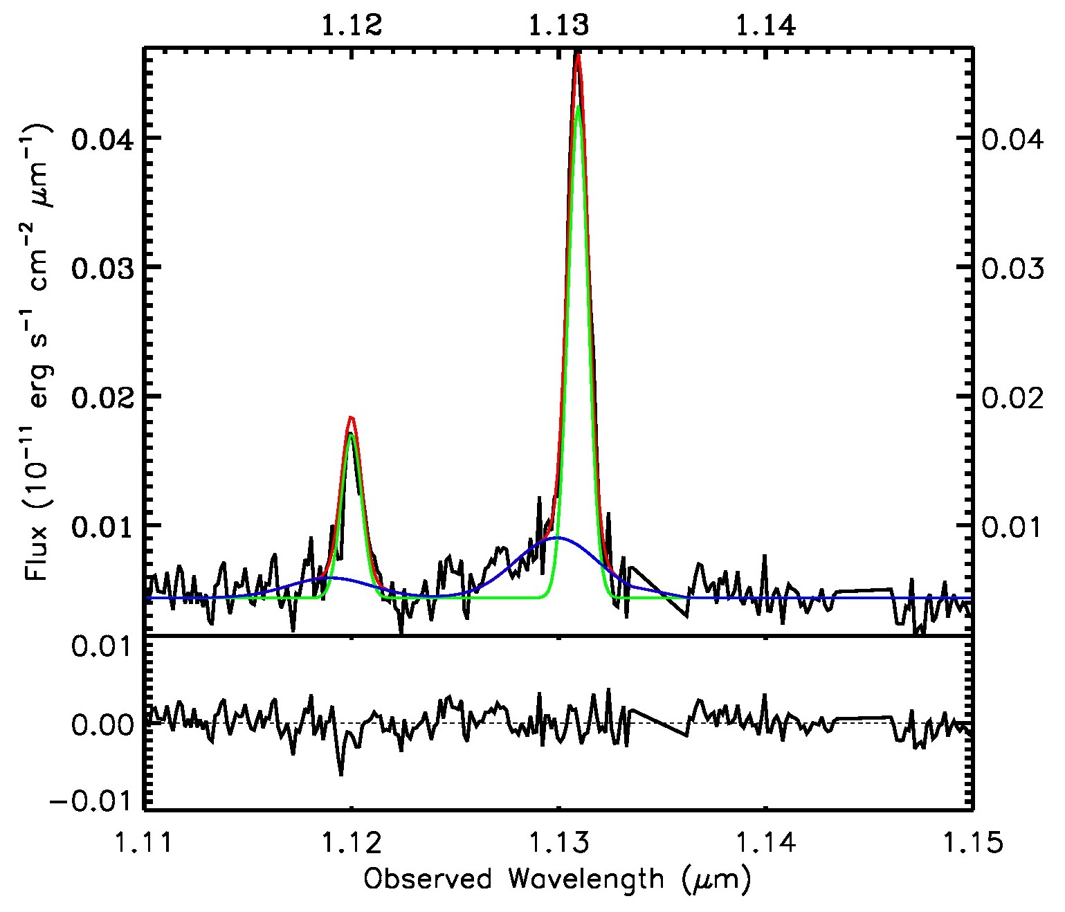
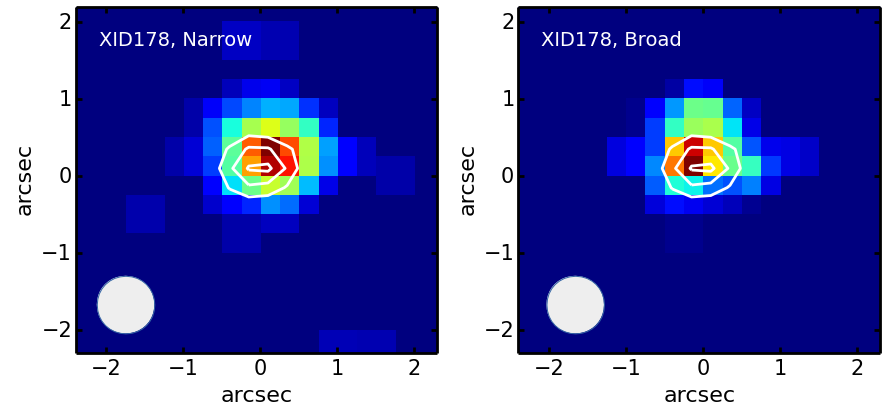
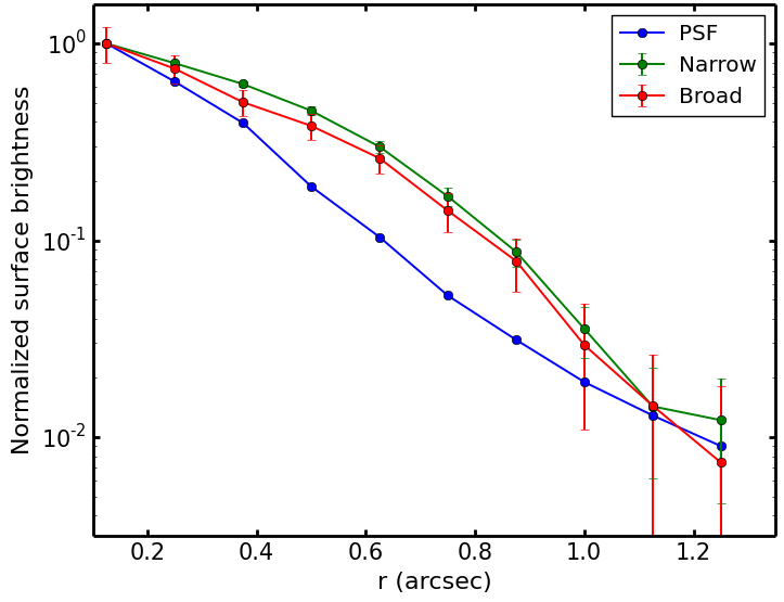
Figure 2: Upper Panel: The J band spectrum of XID178 around the [O iii] $\lambda$4959, 5007 lines extracted from a region of 1.25”$\times$1.25” centered at the QSO position. The observed spectrum is shown in black, the red curve shows the full fit, the green curve shows the narrow line component while the blue curve shows the broad line component. The residuals of the fit are shown in the smaller panel below the integrated spectrum. Middle panel: maps of the narrow (left) and broad (right) component in the [O iii] $\lambda$5007 profile for XID178. Each pixel corresponds to a spatial scale of 0.25” which at the redshift of this object is equivalent to 2.15 kpc.The white contours in these maps represent the respective continuum emission of the object at levels 50%, 75% and 95%. North is up and East is left. The maps show a one pixel offset between the narrow and the broad components. The gray circle on the lower left shows the size of PSF.  Lower panel: Surface brightness profiles of the individual Gaussian components in XID178 derived from the flux maps in the middle panel. Green curve denotes the narrow component, red curve the broad component and the blue curve is the PSF of the observations. Both components show an extension up to a distance of 1”.

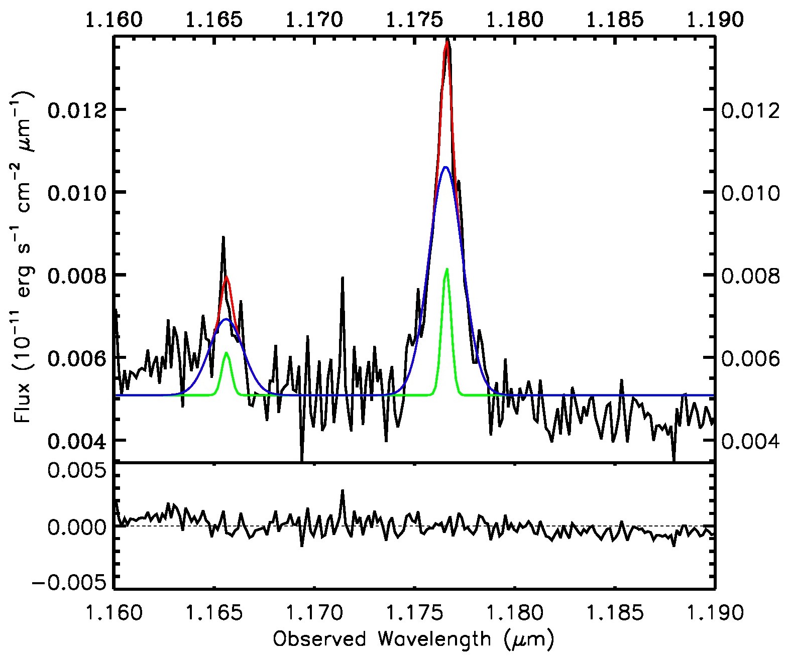
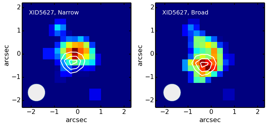
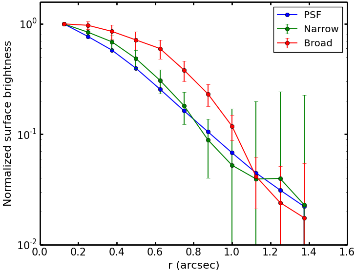
Figure 3: Upper Panel: The J band spectrum of XID5627 around the [O iii] $\lambda$4959, 5007 lines extracted from a region of 1”$\times$1” centered at the QSO position. The color coding for the plot is the same as that of XID178 in Fig. 2. The residuals of the fit are shown in the smaller panel below the integrated spectrum. Middle panel: maps of the narrow (left) and broad (right) component in the [O iii] $\lambda$5007 profile for XID5627. Each pixel corresponds to a spatial scale of 0.25” which at the redshift of this object is equivalent to 2.16 kpc.The white contours in these maps represent the respective continuum emission of the object at levels 50%, 75% and 95%. North is up and East is left. The maps show a significant offset between the spatial locations of narrow and broad emission.The gray circle on the lower left shows the size of PSF.  Lower panel: Surface brightness profiles of the individual Gaussian components in XID5627 derived from the flux maps in the middle panel. Green curve denotes the narrow component, red curve the broad component and the blue curve is the PSF of the observations. Only the broad component shows an extension. The narrow component is point-like since it is consistent with the profile of the PSF star.

XID178 and XID5627 are the candidates in our sample (apart from XID2028 which was published in Cresci et al., 2015) which show definite evidence for the presence of outflow from the [O iii] $\lambda$5007 profile. At a redshift of 1.253 and 1.337, both targets were observed using the J grating of SINFONI to sample the [O iii] lines at $\lambda$ = 4959 $\AA$ and 5007 $\AA$. The total exposure time on source was 3.5 hours for each object achieving a S/N ratio of 34 (XID178) and 11 (XID5627) on the integrated spectrum for the [O iii] $\lambda$5007 line. Due to the low S/N of the [OIII]$\lambda$4959 profile in both targets, the analysis has been restricted to [O iii] $\lambda$5007 only. Table 2 lists the results of the line fitting procedure described in Sec. 4. Figs. 2 and 3 show the integrated spectrum, the flux maps corresponding to narrow and broad Gaussian components and the surface brightness profiles of XID178 and XID5627 respectively.

In order to obtain the flux maps and therefore determine the spatial distribution of the outflow, we re-binned the reduced cube by clustering a 2$\times$2 group of pixels into a single pixel for both the targets. This increases the S/N and allows for a better line fitting across the spaxels. As a result, the re-binning procedure increases the spatial scale of the pixel by a factor of 2 to 2.15 kpc and 2.16 kpc for XID178 and XID5627 respectively.

The [O iii] $\lambda$5007 profile in the integrated spectrum of XID178 in Fig. 2, top panel shows a clear blue wing which traces outflowing gas moving towards us. The velocity offset between the narrow and the broad line Gaussian component is about -275 km/s. The blue wing is not present in the [O iii] $\lambda$4959 profile, but we notice that its location coincides with a significant telluric absorption line as can be seen in the residual spectra. Moreover, as mentioned earlier, the [O iii] $\lambda$4959 profile has too low a S/N to draw any conclusions about the presence of an outflow. Unfortunately, the presence of a red wing in [O iii] $\lambda$5007 cannot be verified since this region of the spectrum is also affected by telluric absorption features as well.

The location of the outflow is apparent from the spatial offset between the narrow and the broad component maps in Fig. 2, middle panels. The white contours in the figure represent the location of the continuum emission. The broad emission appears slightly shifted towards east with respect to the continuum as well as the narrow profile. The surface brightness profiles of these individual components in Fig. 2, bottom panel confirm that they are extended since there is an excess in the [O iii] $\lambda$5007 emission compared to the PSF profile up to 1” ($\sim$ 8.6 kpc).

The integrated spectrum of XID5627 around the [O iii] $\lambda$4959,5007 is shown in Fig. 3, top panel. The [O iii] $\lambda$5007 line profile is nearly symmetric, though two Gaussian components were required to reproduce the overall extended line profile, with a velocity offset of about -9 km/s between the narrow and the broad Gaussian components. The line profile thus suggests that the ionized gas might be moving both towards and away from the observer.

The middle panels of Fig. 3 show the map tracing the narrow and the broad components of [O iii] $\lambda$5007 profile in XID5627. There is a clear offset between the spatial locations of the narrow and broad component emissions. In addition, the narrow component is point-like since it is consistent with the PSF profile, while the broad component is extended up to a distance of 1” ($\sim$ 8.40 kpc) from the center (Fig. 3, bottom panel).

The outflow velocities have been estimated from the integrated spectrum as described in Sec. 4. The values from the different prescriptions are tabulated in Table 3. The error values are 1$\sigma$ errors computed by creating 100 mock spectra as described in Sec. 4. The velocity values cover the range $\sim 490-730$ and $\sim 250-520$ km/s for XID178 and XID5627 respectively. Clearly, these ranges of velocities will imply a range in the outflow properties calculated in Sec. 6, as discussed in Sec. 7.

	XID178	XID5627	XID5330	XID54204
$\mathrm{v_{10}^{a}}$	-493 $\pm$ 27	-247 $\pm$ 21	-258 $\pm$ 21	-1265 $\pm$ 32
$\mathrm{w_{80}^{a}}$	730 $\pm$ 60	517 $\pm$ 29	659 $\pm$ 21	1879 $\pm$ 135
$\mathrm{v_{10}^{b}}$	-665 $\pm$ 31	-265 $\pm$ 28	–	-963 $\pm$ 584

Table 3: The velocity values derived from the integrated spectrum. $\mathrm{v_{10}}$ denotes the 10th percentile velocity value, $\mathrm{w_{80}}$ denotes the velocity width containing 80% of the flux.

5.2 XID5330

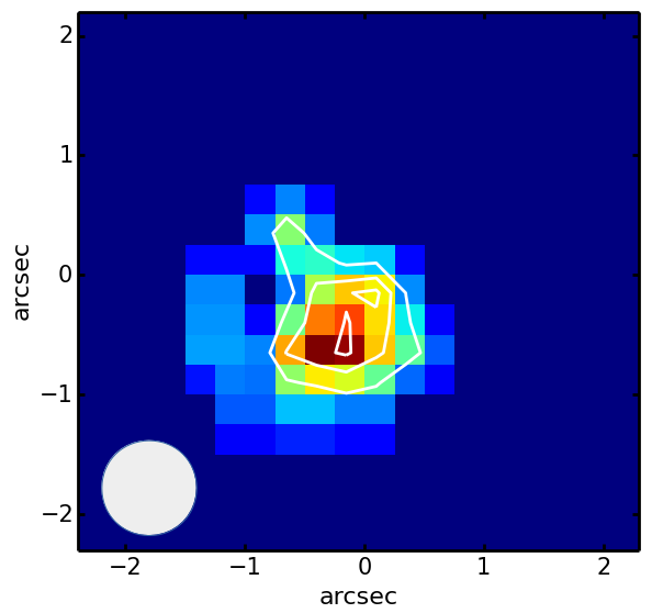
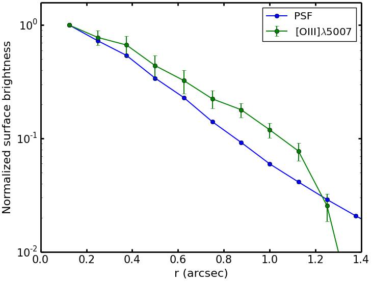
Figure 4: Top left:The H band spectra of XID5330 around [O iii] $\lambda$4959,5007 lines extracted from a region of 1”$\times$1” centered at the QSO position. The observed spectrum in shown in black and the full fit model is shown in red. Due to low S/N on the spectra, only a single Gaussian component was used for line fitting. The lower panel shows the residuals of the line fit. Top right: Map tracing the Gaussian component in [O iii] $\lambda$5007 profile of XID5330. The white contours show the continuum levels at 50%, 75% and 95%. Each pixel corresponds to a spatial scale of 0.25” ($\sim$2.12 kpc). North is up and east is towards left. The gray circle on the lower left shows the size of PSF. Bottom panel: The surface brightness profile of the narrow component of the map in the top right panel compared to the PSF profile. The [O iii] $\lambda$5007 emission is extended up to 1.1” ($\sim$ 9.5 kpc).

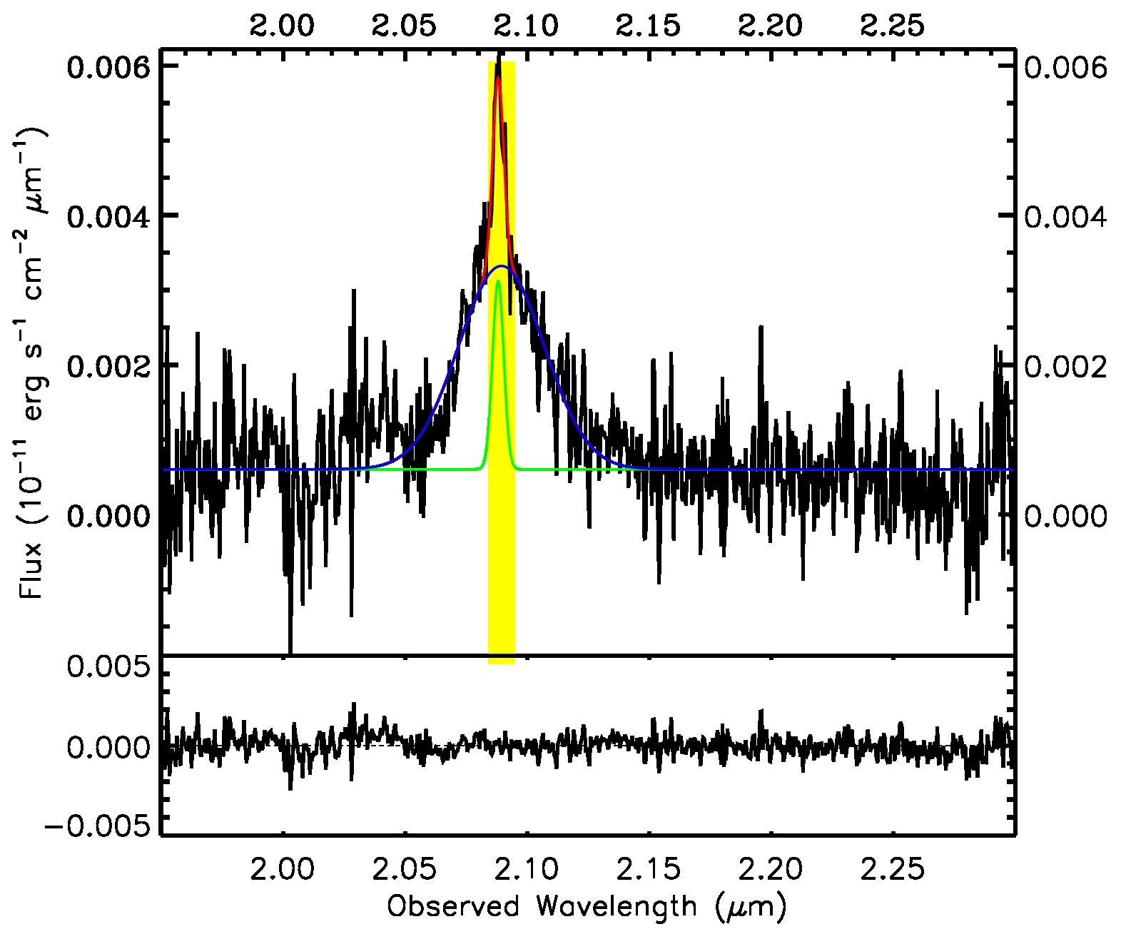
Figure 5: The K band spectra of XID5330 around H$\alpha$ line extracted from a region of 1”$\times$1” centered at the QSO position. There are two distinct components of overall H$\alpha$ line profile: a narrow component, shown in green and a broad component, shown in blue. The overall fit is shown in red. The lower panel shows the residual of this line fit.

XID5330 has the shortest integration time among the targets of our program. The spectral resolution is lower compared to the rest of the sample since the observations were taken in the SINFONI H+K band. At a redshift of 2.169, the [O iii] line falls in the H band at a wavelength of 1.593 $\mu$m and we also detect H$\alpha$ line at 2.088 $\mu$m in the K band. In $\sim$50 minutes, we were able to reach a S/N of 5 for [O iii] $\lambda$5007 and 8.3 for H$\alpha$ in the integrated spectrum.

The integrated H band spectrum around the [O iii] $\lambda$4959,5007 lines is shown in Fig. 4, top left panel. We have a low S/N ratio for the [O iii] $\lambda$5007 profile and hence only one Gaussian has been used for line fitting. Fig. 4, top right panel shows the map tracing the narrow component which shows an extension of $\sim$1.1” , which translates to a spatial scale of 9.5 kpc from the centre, when compared to the PSF profile (Fig. 4, bottom panel). The absence of a broad Gaussian component coupled with low spectral resolution and low S/N on the spectrum does not allow us to compute mass outflow rates and the associated kinetic power as done for other objects in the sample.

The K band spectrum around the H$\alpha$ line profile, shows a clear distinction between the narrow and broad H$\alpha$ components in the spectrum (see Fig. 5, left panel). The line fitting parameters for H$\alpha$ are given in Table 4. The broad component of H$\alpha$ has a velocity dispersion of $\sim$ 6000 km/s and is clearly AGN related. The velocity offset between the narrow and the broad Gaussian components is about +190 km/s (the broad component is redshifted with respect to the narrow component). The low S/N of the spectra does not allow us to disentangle contributions (if any) to the flux from [NII]$\lambda$6549,85 lines which are expected to lie at 2.0837$\mu$m and 2.0951$\mu$m respectively i.e. on either side of the narrow H$\alpha$ component.

Parameter	Value
$\mathrm{\lambda_{narrow}}$	2.0881 $\pm$ 0.0005 $\mu$m
$\mathrm{v_{narrow}}$	770 $\pm$ 282 km/s
$\mathrm{\lambda_{broad}}$	2.0894 $\pm$ 0.0005 $\mu$m
$\mathrm{v_{broad}}$	5950 $\pm$ 808 km/s

Table 4: Line fitting parameters for K band spectra of XID5330. Two components, narrow and broad Gaussian were used to fit the entire H$\alpha$ profile. $\mathrm{\lambda_{narrow}}$ = central wavelength of the narrow Gaussian component; $\mathrm{v_{narrow}}$ = velocity corresponding to the FWHM of the broad Gaussian; $\mathrm{\lambda_{narrow}}$= central wavelength of the broad Gaussian component and $\mathrm{v_{broad}}$ = velocity corresponding to the FWHM of the broad Gaussian component. The wavelength of the broad component is redshifted by 190 km/s with respect to the narrow component.

The presence of the broad H$\alpha$ line gives us the possibility to estimate and verify the mass of the black hole. We use the Greene & Ho (2005) formalism wherein the black hole mass from the H$\alpha$ line is given by:

$$m_{bh}^{H\alpha}=2.0\times 10^{6}\left(\frac{L_{H\alpha}}{10^{42}\leavevmode\nobreak\ \mathrm{erg\leavevmode\nobreak\ s^{-1}}}\right)^{0.55}\left(\frac{FWHM_{H\alpha}}{1000\leavevmode\nobreak\ \mathrm{km\leavevmode\nobreak\ s^{-1}}}\right)^{2.06}M_{\odot}$$ (2)

We consider only the broad line component of the flux of the H$\alpha$ profile for the estimation of luminosity, which comes out to be $\mathrm{2.7\pm 1.0\times 10^{43}}$ erg/s. Using the values from Table 4 and the luminosity of the broad component, we arrive at a black hole mass of 8.9$\pm$0.2 $\times$ 10⁸ M_⊙. This is a factor of $\sim$5 larger than the value given in Table 1, which is based on broad MgII line. This discrepancy might be due to the low S/N in both optical as well as H+K band data. Moreover, we are unable to disentangle the contribution due to [NII]$\lambda$6549,85 on the entire H$\alpha$ profile which, if present, could bring down our mass estimate.

5.3 XID54204

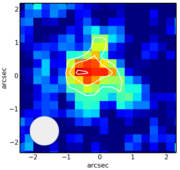
Figure 6: Left panel: The J band spectrum of XID54204 around [O iii] $\lambda$5007 line extracted from a region of 1”$\times$1” centred at the QSO position. The color codes for different part of the spectra are defined in the same way as Fig. 2, top panel. Right Panel: Continuum collapsed channel map around the narrow component of [O iii] $\lambda$5007 line (yellow region in the left panel, 1.180-1.182 $\mu$m). Each pixel corresponds to a spatial scale of 0.25” which at the redshift of this object is equivalent to $\sim$2.16 kpc. The white contours indicate the peak of the [O iii] $\lambda$5007 emission at levels 50%, 75% and 95%. North is up and East is towards left. The gray circle on the lower left shows the size of PSF. 

XID54204 has a very faint [O iii] $\lambda$5007 signal despite an integration time of 3.5 hours on the target. The [O iii] $\lambda$5007 line is detected at a wavelength of 1.1796 $\mu$m consistent with the object being at z$=$1.356. A S/N of 4.4 could be reached in the integrated spectrum of the [O iii] $\lambda$5007 emission line.

Although faint, the [O iii] $\lambda$5007 profile in the integrated spectrum is quite broad, so a single Gaussian is not able to provide a good fit of the line profile. Therefore we added a second component and the resulting integrated spectrum is given in Fig. 6, left panel. The integrated spectrum indicates the presence of a blue wing in the [O iii] $\lambda$5007 profile, hence the outflow direction is towards the observer. The velocity offset between the narrow and the (blue-shifted) broad Gaussian component is $\sim$360 km/s.

Fig. 6, right panel shows the continuum subtracted [O iii] $\lambda$5007 line core map, confirming [O iii] emission from this object. The line core map was obtained by integrating the continuum collapsed SINFONI data cube between 1.180-1.182 $\mu$m, shown by the yellow region in the integrated spectrum in Fig. 6. Due to low S/N in each spaxel, one cannot do line fitting across the FOV and consequently we could not obtain surface brightness profiles as we did for other objects. In this case, one can only put an upper limit of the spatial extension of the outflow from the FWHM of the PSF, which is 0.8” ($\sim$ 6.9 kpc). The outflow velocity from the integrated spectrum have been estimated in the range $\sim$950-1900 km/s (see Table 3).

6 Outflow properties

The determination of the properties of the outflow such as its mass is complicated by the fact that the outflow has a multi-phase nature. While we are tracing the outflow in its warm ionized phase using the [O iii] $\lambda$5007 line, a significant fraction of the outflows are believed to be in the cold molecular gas phase (Veilleux et al., 2013; Cicone et al., 2014; Feruglio et al., 2015; Brusa et al., 2015b; Nyland et al., 2013). There are many papers in the literature which discuss the estimation of the mass of the ionized outflows from either H$\beta$ or [O iii] $\lambda$5007 (e.g., Holt et al., 2011; Cano-Díaz et al., 2012; Liu et al., 2013; Harrison et al., 2014). Due to the limited information available to us (e.g., lack of Balmer lines), we derive the outflow gas mass from the [O iii] $\lambda$5007 line based on Cano-Díaz et al. (2012). [O iii] lines are very sensitive to temperature and ionization but poor tracers of mass, hence the current analysis only provides (at best) an order-of-magnitude estimate of the outflow properties.

Below, we summarize the essential formulas used to arrive at the outflow properties and the assumptions associated with them. The mass of the ionized outflowing gas is given by:

$$M_{ion}^{out}\approx 5.33\times 10^{8}\left(\frac{C}{10^{[O/H]-[O/H]_{\odot}}}\right)\left(\frac{L[{O\textsc{iii}}]}{10^{44}\leavevmode\nobreak\ \mathrm{erg\leavevmode\nobreak\ s^{-1}}}\right)\left<\frac{n_{e}}{100\leavevmode\nobreak\ \mathrm{cm^{-3}}}\right>^{-1}M_{\odot}$$ (3)

where C (= ¡n_e¿²/¡n${}_{e}^{2}$¿) $\sim$ 1 based on the hypothesis that all the ionizing gas clouds have the same density, L[O iii] is the luminosity of the [O iii] $\lambda$5007 line tracing the outflow, n_e is the electron density of the outflowing gas and 10${}^{[O/H]-[O/H]_{\odot}}$ represents the oxygen abundance in Solar units. The luminosity of [O iii] $\lambda$5007 is derived from the flux of the broad line component in the integrated spectrum, when present. In the absence of a broad component, mass estimate of the outflowing gas could not be obtained. The normalization factor in Eq. 3 is dependent on the emissivity of the ionized gas which is further dependent on electron density and the temperature of the gas. The emissivity calculations were done using PyNeb (Luridiana et al., 2015). The following assumptions go into Eq. 3:

• Most of the oxygen in the outflow is in its ionized form, O⁺² i.e. n(O⁺²) $\approx$ n(O).

• The number density of atomic helium is 10% that of atomic hydrogen i.e. n(He) $\approx$ 0.1 n(H). This is based on the ”cosmic composition” from abundance measurements in the Sun, meteorites and other disk stars in the Milky Way (Ferrière, 2001).

• The electron density, n_e is assumed to be equal to 100 cm^-3. The electron density is usually measured using the line ratio of the [S ii] $\lambda$6716,31 doublet (Peterson, 1997). As a recent example of this technique, Perna et al. (2015a) estimate n${}_{e}\approx$ 120 cm^-3 from the [S ii] doublet in the outflow component for a high S/N target XID5321 in the COSMOS field which is within the typical value estimates of electron density for the NLR ($\mathrm{\lesssim 50-1500\leavevmode\nobreak\ cm^{-3}}$). Previous works also use a value within this range when the electron density is not known. For example, Cano-Díaz et al. (2012) use a value of 1000 cm^-3, while Cresci et al. (2015) and Liu et al. (2013) assume a value of 100 cm^-3 and Harrison et al. (2014) and Carniani et al. (2015) use a value of 500 cm^-3. We have taken these differences into account while comparing the outflow rates we derive to the previous works in Sec. 7. We also discuss the level of uncertainties due to these assumptions.

• Emission lines from a single ion having different excitation potentials are highly temperature dependent which makes them suitable for electron temperature measurement in the NLR (Peterson, 1997). As mentioned before, the normalization factor in Eq. 3 depends on the emissivity of the ionized gas which is sensitive to temperature changes. Hence the normalization factor in Eq. 3 will change with the assumed temperature. Usually, [O iii] $\lambda$4363,4959,5007 or [NII]$\lambda$5755,6548,6583 are the set of lines used for this purpose. Typical temperatures measured for the NLR using this method come out to be about 10,000-25,000 K. For our calculations, we assume a value of 10,000 K.

• Since the current data do not allow us to determine oxygen abundances, solar metallicity values have been used.

Due to the limited information available to us about the morphology of the outflow, we assume a simple conical outflow model for our objects. The volume averaged density of the outflowing gas, ¡$\mathrm{\rho_{out}}$¿ (not to be confused with the gas density of individual clouds) is given by:

$$<\rho_{out}>=3\frac{M_{out}}{\Omega\cdot R_{out}^{3}}$$ (4)

where $\Omega$ is the solid angle subtended by the (bi)-conical outflow and $\mathrm{R_{out}}$ is the extension of the outflow in the cone. The mass outflow rate is then given by $\mathrm{\dot{M}_{out}\approx<\rho_{out}>_{V}\cdot\Omega R_{out}^{2}\cdot v_{out}}$. When combined with Eq. 3, this gives:

$$\begin{split}\dot{M}_{ion}^{out}\approx&\leavevmode\nobreak\ 1.64\times 10^{3}\cdot\left(\frac{1}{10^{[O/H]-[O/H]_{\odot}}R_{kpc}}\right)\left(\frac{L[{O\textsc{iii}}]}{10^{44}\leavevmode\nobreak\ \mathrm{erg\leavevmode\nobreak\ s^{-1}}}\right)\\ &\left(\frac{v}{1000\leavevmode\nobreak\ \mathrm{km\leavevmode\nobreak\ s^{-1}}}\right)\left<\frac{n_{e}}{100\leavevmode\nobreak\ \mathrm{cm^{-3}}}\right>^{-1}M_{\odot}/yr\end{split}$$ (5)

where v is the velocity of the outflowing gas (from Table 3) out to a radius $\mathrm{R_{kpc}}$ in units of kiloparsec. The kinetic energy of the outflow due to the ionized component is simply $\mathrm{1/2\dot{M}_{out}^{ion}v^{2}}$:

$$\begin{split}\dot{E}_{K}^{ion}=&\leavevmode\nobreak\ 5.17\times 10^{44}\cdot\frac{1}{10^{[O/H]-[O/H]_{\odot}}R_{\mathrm{kpc}}}\left(\frac{L[{O\textsc{iii}}]}{10^{44}\leavevmode\nobreak\ \mathrm{erg\leavevmode\nobreak\ s^{-1}}}\right)\cdot\\ &\left(\frac{v}{1000\leavevmode\nobreak\ \mathrm{km\leavevmode\nobreak\ s^{-1}}}\right)^{3}\left<\frac{n_{e}}{100\leavevmode\nobreak\ \mathrm{cm^{-3}}}\right>^{-1}\mathrm{erg\leavevmode\nobreak\ s^{-1}}\end{split}$$ (6)

If the distance of the outflowing region is known from the maps, we can also compute the dynamical time scale of the outflow:

$$t_{d}\approx R_{out}/v_{out}$$ (7)

where $\mathrm{v_{out}}$ is the outflow velocity inferred from the kinematic analysis. The dynamical time scales could give us an idea about the ”on” phase of the outflow, which, whenever possible to calculate, would be a direct observational constraint on the time scales of the outflow driven by an AGN at high redshift. The outflow properties mentioned in this section have been derived for every object in our sample and are reported in Table 5. The Table indicates a range of these properties obtained using the velocity ranges in Table 3, keeping other assumptions such as the electron density, temperature, radius and metallicity constant. The errors on these properties have been ignored compared to the systematic uncertainties.

Object ID	$\mathrm{f_{[{O\textsc{iii}}]}}$	log($\mathrm{L_{[{O\textsc{iii}}]}}$)	$\mathrm{M_{out}^{ion}}$	$\mathrm{\dot{M}_{out}^{ion}}$	$\mathrm{\dot{E}_{K}^{ion}}$	$\mathrm{P_{SFR}}$
	(10-16 erg/s/cm-2)	(erg/s)	(107 M${}_{\odot})$	(M⊙/yr)	(1041 erg/s)	(1043 erg/s)
(1)	(2)	(3)	(4)	(5)	(6)	(7)
178	2.33 $\pm$ 0.16	42.35 $\pm$ 0.02	1.13	2.00-2.96	1.53-4.98	9.4
5330*	1.29 $\pm$ 0.04	42.68 $\pm$ 0.01	–	–	–	7.0
5627	1.65 $\pm$ 0.15	42.27 $\pm$ 0.02	0.94	0.83-1.74	0.16-1.46	11.0
54204	1.54 $\pm$ 0.84	42.26 $\pm$ 0.05	0.91	3.91-7.63	11.44-84.95	30.7
2028†	2.64 $\pm$ 0.09	42.66 $\pm$ 0.01	2.32	8.24	58.44	17.5

Table 5: Outflow properties derived from the line fits and the formulas mentioned in Sec. 6. (1) The X-ray ID of the sample; (2) Flux of the broad Gaussian component in the [O iii] $\lambda$5007 profile; (3) luminosity corresponding the flux in (2); (4) is the outflow mass traced by the [O iii] $\lambda$5007 line, (5) & (6) are the range in mass outflow rates and the kinetic energy associated with the ionized component corresponding to the velocity values in Table 3, keeping the rest of the assumptions constant; (7) Power due to the star formation in the host galaxy.

7 Discussion

7.1 Outflow detection and selection efficiency

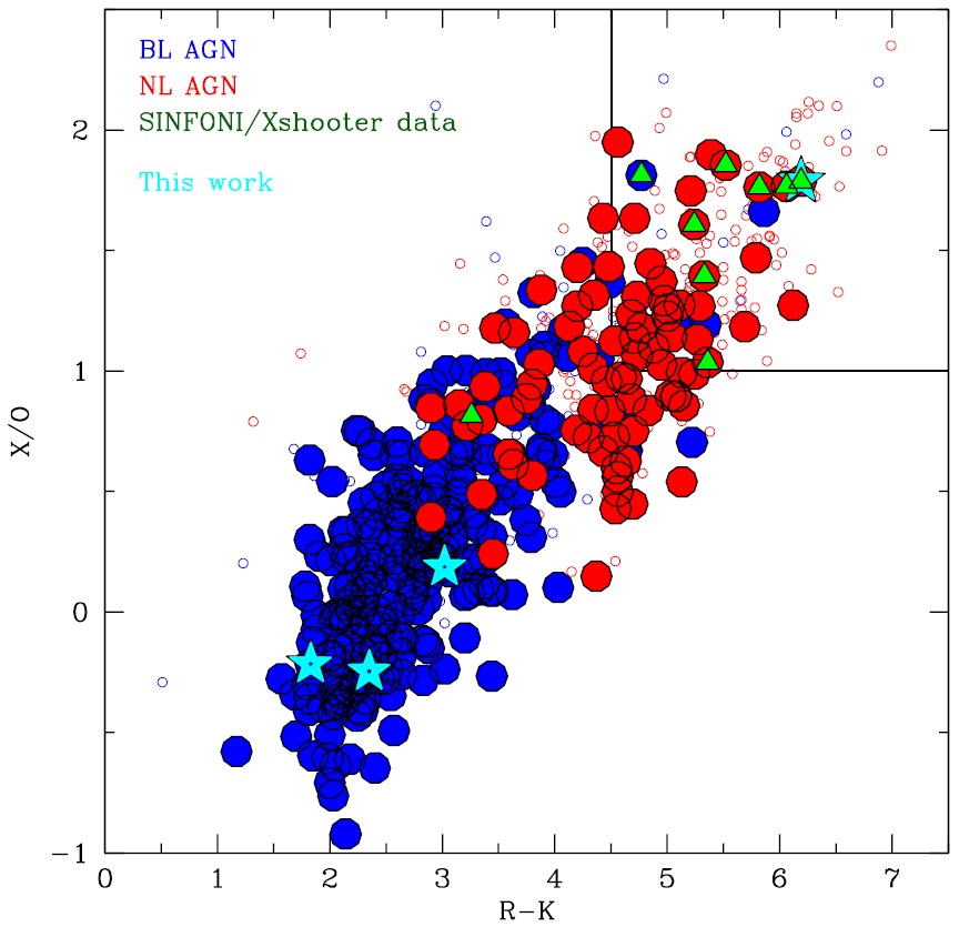
Figure 7: X-ray to optical flux ratio (X/O) vs. R-K (Vega) color magnitude plot. Open circles represent all the data points from the XMM-COSMOS survey, red and blue filled circles represent the spectroscopically confirmed narrow line and broad line AGNs respectively. In green are the AGN with detected outflows published in Brusa et al. (2015a); Perna et al. (2015b). Data points in starred cyan represent the objects from this paper. Clearly, with our sample, we are exploring a different region of the plane.

At least three of the four targets (XID178, XID5627 and XID54204) presented in this paper show clear evidence of outflows. The S/N ratio of XID54204 is very low so the spatial information of the outflow could not be derived, although there is an indication of the presence of a blue wing in its [O iii] $\lambda$5007 profile in the integrated spectrum. The low S/N of XID54204 could be simply due to the high air mass through which this object was observed (see Sec. 3). Due to the low integration time of XID5330 coupled with a lower spectral resolution in the H+K band of the SINFONI grating, we were not able to reach the S/N ratio limit for which we could observe the wings in the [O iii] $\lambda$5007 profile. Including XID2028 (Cresci et al., 2015) which also satisfies the selection criterion of our sample, we can say that Fig. 1 is an effective tool to select AGN in an outflowing phase. Our study reinforces previous evidence for absorption variability in the X-ray spectra of AGN close to the forbidden region (Vasudevan et al., 2013). In order to populate this plane with other known outflows, we have added in Fig. 1 the sample from Brusa et al. (2015a) for which we have the hydrogen column density and Eddington ratio estimates (red circles). We see that three out of the four objects of that sample lie inside or very close to the forbidden region which further points to the efficiency of this selection procedure.

Previous studies on AGN outflows have been biased in pre-selected targets with higher chances to be in an outflowing phase, similar to what we did. As an example, the Brusa et al. (2015a) selection was based on the fact that the QSOs in an outflowing phase are expected to be dusty and reddened, the so-called ”red QSOs”. This is shown by the red circles in Fig. 7 which shows a plot between the X-ray (2-10 keV) to optical flux ratio (X/O) and R-K (Vega) colors. Three of our targets (marked by blue stars) lie in the blue QSO region (R-K $\sim$ 2). XID54204 is not included in this figure as it is not detected in the 2-10 keV band. XID2028 is the blue star in the red QSO region. We are therefore exploring a completely different region of the X/O vs. R-K plot and we find that the objects in the blue region also show outflows. Clearly the next step would be to test these selection criteria with a blind sample which covers the whole plane in Fig. 7 (and Fig. 1).

The one dimensional spectra of three of the objects from our sample (XID2028, XID5627 and XID54204 a.k.a XCOS2028, XCOS5627 and COS178 respectively) have also been presented in Harrison et al. (2016) as part of the KMOS AGN survey at High Redshift (KASHz). Except for XID54204, our one dimensional results (line wavelengths, widths and luminosity) are compatible with those reported by Harrison et al. (2016). The minor differences might be due to the different apertures used for spectral extraction from the IFU cube and the errors associated with the flux calibration. Harrison et al. (2016) do not detect any [O iii] $\lambda$5007 in their analysis for XID54204 (COS178). We were able to detect the presence of the faint [O iii] $\lambda$5007 signal by constructing a continuum subtracted channel map over the narrow component of the line as given in Fig. 6.

7.2 Source of the outflows

In order to understand the nature of ionized outflows, we need to estimate the total mass of the outflowing gas, the mass outflow rate and the kinetic power driven by the AGN using the formulas given in Sec. 6. As mentioned in Sec. 5, we explore a range of outflow properties depending on the velocity measurements. Tight correlations are expected between these quantities and the bolometric luminosity of the AGN according to theoretical models which also predict high velocity outflows from AGN (King et al., 2011; Zubovas & King, 2012). These models predict outflow velocities in the range $1000-1500$ km/s and mass outflow rates up to 4000 M_⊙/yr which are extended to kiloparsec scales. XID2028 shows outflow velocities up to 1500 km/s extended up to 13 kpc from the central object with the total mass outflow rate expected to be at least 1000 M_⊙/yr (Cresci et al., 2015). Such high velocities could not be sustained by star formation alone and a more powerful source such as an AGN is required. This is also the case for XID54204 where we observe linewidths with velocity exceeding 1000 km/s. XID178 and XID5627 also show outflows which are spatially extended up to $\sim$ 8.6 kpc. Compared to XID2028 and XID54204, these objects have lower outflow velocities up to $\sim$700 km/s. However, these are projected velocities and depending on the inclination of these systems, the actual velocities may be higher than the reported values. Nevertheless, these velocities are compatible with star-formation processes.

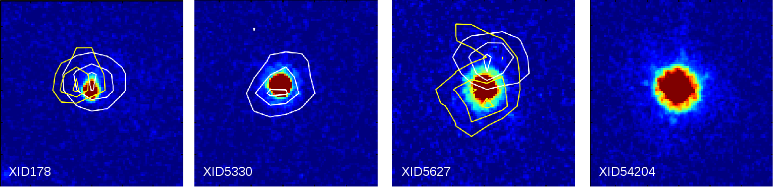
Figure 8: 3”$\times$3” HST-ACS images of the sample presented in this paper, with a spatial scale of 3”$\times$3” for each object. For XID178 and XID5627, the white contours represent the narrow component of the [O iii] $\lambda$5007 emission line profile while the yellow contours represent the broad component while for XID5330, the white contours represent the single Gaussian component of [O iii] $\lambda$5007. All contours are at levels 50%, 75% and 95%. The SINFONI data are not corrected for astrometry.

We looked at the Hubble Space Telescope (HST) images for these objects, and the cutouts are shown in Fig. 8. All images have a spatial scale of 3${}^{\prime\prime}\times$3^′′ which is comparable to the flux and velocity maps presented in Sec. 5. None of these images show any disturbed morphology that could hint to a recent merger, therefore we may disfavor the idea that the dynamical signatures interpreted as outflows are actually due to mergers. The white contours in Fig. 8 represent the narrow [O iii] $\lambda$5007 emission for XID178, XID5330 and XID5627 while the yellow contours represent the broad component. It is clear from the figure that the ionized emission traces a larger fraction of the total gas in the host galaxy compared to the optical images.

Based on the star formation rates (SFR) of the host galaxies of our sample of QSOs, we can also derive the kinetic power driven by supernovae and stellar winds and compare it to the outflow power we obtain to identify the possible source for such outflows. The power driven due to these stellar processes can be calculated using Veilleux et al. (2005) formalism:

$$P_{SF}=7\cdot 10^{41}\times SFR\leavevmode\nobreak\ \leavevmode\nobreak\ \mathrm{M_{\odot}/yr}$$ (8)

The power due to star formation for each of our targets are listed in column 7 of Table 5 and can be compared with the kinetic power of the outflow due to the ionized gas component given in column 6 of the same table. For XID2028, Cresci et al. (2015) reported a value of $\mathrm{\sim 1.5\times 10^{44}\leavevmode\nobreak\ erg/s}$ for the kinetic energy due to the ionized gas as traced by the H$\beta$ line, while we obtain $\mathrm{\sim 5.8\times 10^{42}erg/s}$ from the [O iii] $\lambda$5007. The apparent discrepancy of a factor of 25 shows the difficulty of using [O iii] lines as tracer of the outflow mass as explained in Sec. 6. For reference, we use both the values we obtain using [O iii] $\lambda$5007 and that obtained by Cresci et al. (2015) using H$\beta$ in the plots to follow to demonstrate the differences in power estimates from the two lines. Note that all the mass outflow rates reported in Table 5 are lower limits because additional gas phases are missing.

In Fig. 9 we compare the outflow kinetic power with the predicted energy input rate from star formation following Veilleux et al. (2005) for our sample and other previous studies (Harrison et al., 2014; Brusa et al., 2015a; Cresci et al., 2015). The outflow kinetic energy was recomputed for each work from the literature to be consistent with our assumption of electron density (100/cm³) and temperature (10,000 K). The solid, dashed and dotted lines represent 100%, 5% and 0.1% ratios, respectively. For the two newly detected outflows (XID178 and XID5627, red stars in the figure) having $>0.1\%$ coupling between the stellar energy input and the ISM is sufficient to make star-formation viable as a dominant power source for the observed outflows. For XID54204, star formation itself could not sustain the observed high velocities and kinetic power (King et al., 2011).

In Fig. 10 the outflow kinetic energy is plotted against the AGN bolometric luminosity. We included in the figure other known ionized (Greene et al. 2012; Harrison et al. 2014; Carniani et al. 2015; Brusa et al. 2015a; Cresci et al. 2015) and molecular (squares, Cicone et al. 2014; Sun et al. 2014; Feruglio et al. 2015) outflows. The dotted, dashed and the solid lines represent the fraction of AGN bolometric luminosity in the form of the outflow power (0.1%, 5% and 100% respectively). Two of the objects presented in this work (XID178 and XID5627, red stars at lower bolometric luminosity) lie at the low energy end of the distribution of previously reported ionized outflows, while XID54204 (red stars at a higher bolometric luminosity) falls in the regime of previously known ionized outflows. Theoretical models predict a coupling of $\sim$0.1-5% for AGN-driven outflows (King, 2005), and for these three objects a coupling less than $0.1\%$ of the radiative power of the AGN with the ISM might be sufficient to power the detected outflows. It is important to note that due to the multi-phase nature of the outflows, our kinetic energy estimates are lower limit, since one should consider the total mass of the outflow in the form of ionized, molecular and neutral gas. This is supported by the fact that the previously reported molecular outflows fall into a regime with higher coupling ($\sim$5%) between the outflow kinetic energy and energy released by the AGN. The exact conversion factor to go from ionized to the total gas mass is not known and might vary on an object-by-object basis. Clearly follow-up observations at mm wavelengths are needed to have a more complete picture.

Knowing the radius of the outflow for XID178 and XID5627 to be $\sim$8.6 kpc from the surface brightness profiles in Figs. 2 and 3, the dynamical time scale of the outflow calculated from Eq. 7 comes out to be $\approx$ 18 Myr for both targets. This value is similar to previously reported outflow timescales and AGN lifetimes (e.g. Cresci et al. 2015; Greene et al. 2012; Martini & Weinberg 2001). This exercise could not be performed for XID54204 as we do not have the spatial resolution to determine the size of the outflow.

In summary both star-formation processes and AGN radiation could be the dominant power source for the outflows presented in this paper. Although, the observed high kinetic power for XID54204 points to an AGN driven outflow, a higher S/N and better spatial resolution data is required to confirm this.

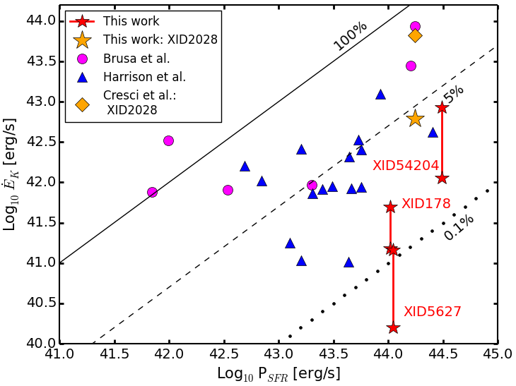
Figure 9: Kinetic outflow power, $\dot{E}_{K}$ vs. the power driven by star formation, $P_{SFR}$. The solid, dashed and dotted lines represent 100%, 5% and 0.1% ratios between the two powers. Our sample is represented by the star symbols while the other data points have been obtained from Brusa et al. (2015a); Cresci et al. (2015) and Harrison et al. (2014). All data points represent outflow powers due to the ionized gas calculated from [O iii] $\lambda$5007 line, except the data point from (XID2028: Cresci et al., 2015) which represents one of the objects from our selection and whose outflow properties were reported using H$\beta$ line. The two points for XID2028 show the differences in power estimates from the two emission lines. The range of kinetic power from our sample is due to the different prescriptions used to derive the outflow velocity.

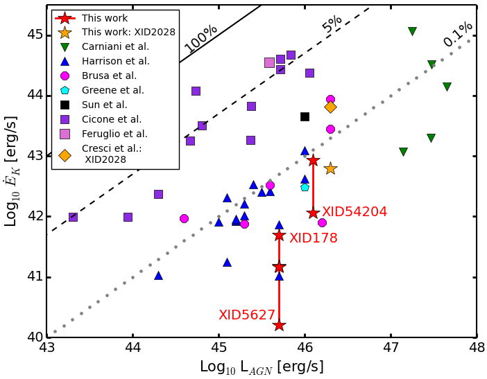
Figure 10: Kinetic outflow power, $\mathrm{\dot{E}_{K}}$ (ionized and molecular) vs. bolometric luminosity of the AGN, L_AGN. The solid, dashed and dotted lines represent 100%, 5% and 0.1% of the total bolometric luminosity of the AGN in the form of the outflow power. The data points from this work are shown in red stars (XID178, XID5627). The molecular outflows are represented by squares (Cicone et al., 2014; Feruglio et al., 2015; Sun et al., 2014), while the rest of the data points represent ionized outflows (Carniani et al., 2015; Harrison et al., 2014; Cresci et al., 2015; Brusa et al., 2015a; Greene et al., 2012). The outflow properties for all the ionized outflows were obtained using [O iii] $\lambda$5007 line except for Cresci et al. 2015 for which analysis from H$\beta$ is shown in this plot to represent the differences in analysis from the two lines for the same data.

The outflow momentum rate, defined as $\mathrm{v_{o}\dot{M}_{o}}$, is another fundamental parameter of the outflow which is crucial to understand if it is momentum or energy conserving (Zubovas & King, 2012; Faucher-Giguère & Quataert, 2012). Theoretical models predict that the momentum of the kpc-scale outflow is boosted by the radiation pressure of the wind from the AGN and the outflow energies are of the order of $\approx\mathrm{20\cdot L_{AGN}/c}$ (AGN radiation pressure momentum) implying an energy conserving outflow (Cicone et al., 2014; Feruglio et al., 2015). XID178 and XID5627 have similar bolometric luminosity, outflow velocity and mass outflow rates (see Table 1 and 5). The ratio of the outflow momentum rate to that of AGN radiation pressure momentum comes out to be much less than 1:1 ($\approx$ 0.01:1), which is also consistent with previously reported ionized gas momentum rates (Carniani et al., 2015). The lower ratio might be due to the discrepancy in the outflow mass rates in the molecular and ionized gas phase.

7.3 Uncertainties in the estimates

Although there is substantial observational evidence that outflows are common in AGNs, the derived quantitites associated to these outflows are affected by significant uncertainties.

We have adopted the most commonly used outflow model, i.e. the bi-conical outflow, to derive the mass outflow rates and hence the power driven by the AGN. Mass outflow rate estimates would change if we considered a shell-like outflow geometry instead. This has been extensively discussed in Cicone et al. (2014) and Maiolino et al. (2012) where it was shown that a shell-like geometry gives a higher outflow rate (by a factor of $\sim$3) relatively to the multi-conical or spherical geometry considered above. Since we do not have a 3D view of these galaxies, the exact outflow morphology of any of the targets could not be inferred. However, with the 2D images in hand, one could assume a bi-conical outflow model in all the objects with XID5627 probably having a wide-angled outflow (inferred from the broad component map in Fig. 3, middle right panel) towards the line of sight of the observer. This suggests that the outflow pattern might vary on an object-by-object basis and might introduce errors due to the assumptions made.

As we have illustrated in Figs. 9 and 10, using different prescriptions for determining outflow velocities introduces a range of outflow properties, the extent of which depends on the emission line profile. In all cases, $\mathrm{w_{80}}$ gives a higher velocity value compared to the $\mathrm{v_{10}}$ on the integrated spectrum and the broad component. For a Gaussian profile $\mathrm{w_{80}}$ is close to the FWHM of the line and relates to the typical velocity of the emitting gas, while $\mathrm{v_{10}}$ gives an estimate of velocity the gas moving towards us at the high velocity end. The outflow model we use do not take into account these differences.

Another important source of uncertainty is the lack of a measurement of the electron density for each single AGN studied. The range of electron density in NLR is believed to be in the range $\leq 50-1500$ $\mathrm{cm^{-3}}$ (Peterson, 1997). Observations of local galaxies have shown that the electron density generally drops with distance from the galactic centre, down to values $\la 50$ $\mathrm{cm^{-3}}$ in the galaxy outskirts (Bennert et al., 2006). The observed outflows in our case are extended to kiloparsec scales, but if the gas is dragged out by an over-pressurized bubble the density could be relatively high. We adopt an average electron density of 100 $\mathrm{cm^{-3}}$, based on recent observations by Perna et al. 2015a of a bright QSO (XID5321) using [S ii] $\lambda$6716,31 for which an electron density of $\sim$120 $\mathrm{cm^{-3}}$ have been reported in the off-nuclear regions. However, this method is not effective in measuring electron densities lower than 100 $\mathrm{cm^{-3}}$ (or greater than 1500 $\mathrm{cm^{-3}}$: Peterson 1997). Moreover it is challenging to resolve the [S ii] doublet near H$\alpha$ in many objects and is usually very faint. Hence, we have limitations from observational point of view in determining the electron densities accurately.

A similar concern applies to the temperature estimates as well. The normalization factors in Eqs. 3-5 could change by a factor of $\sim$10 depending on whether the temperature is assumed to be 10,000 K or 25,000 K since the emissivity changes by this factor.

Other sources of uncertainties come from using different lines for deriving outflow properties (such as [O iii]$\lambda$5007 and H$\beta$) and the multi-phase nature of outflows which has been discussed before. The overall errors in the estimates of mass outflow rates and kinetic energies are therefore large, possibly of the order of a factor $\sim 100$.

Hence, we stress the importance of further detailed observations to constrain the outflow energies and hence accurately determine whether AGN or the star formation could drive such outflows.

8 Summary

We summarize below the main results of this work:

• The selection of AGN in an outflowing phase based on the empirical curve by Fabian et al. (2008) (see Fig. 1) seems effective. We were able to verify the presence of such outflows using a kinematic analysis of the [O iii] $\lambda$5007 line in at least four out of a sample of five objects, three of them reported for the first time in this work (XID178, XID5627 and XID54204) and the fourth (XID2028) already presented in Cresci et al. (2015).

• In XID178 and XID5627, the outflow is extended up to $\sim$8.5 kpc in the host galaxy while for XID54204, the [O iii] $\lambda$5007 emission is not spatially resolved. All the objects show high velocities of $\sim$500-1800 km/s in their integrated spectra. The spatial distribution of [O iii] $\lambda$5007 in XID178 and XID5627 might suggest the presence of different outflow morphology in the galaxies.

• For XID5330 we do not have enough S/N ratio and spectral resolution to trace an extended [O iii] $\lambda$5007 emission (if present).

• HST images of the sample do not show any disturbed morphology, possibly ruling out a merger-driven scenario for the observed outflows.

• Based on the measured kinetic energies of the outflows, both star-formation ($\gtrsim 0.1\%$ coupling) and AGN radiation ($<0.1\%$ coupling) could be the dominant power source. In this work we were able to trace only the ionized phase of the outflows. Follow-up observations of the molecular components could allow us to put stronger constraints on the origin of these outflows.

• The assumptions of current models introduce errors of several orders of magnitude on the outflow properties, which makes it difficult to infer the source of these outflows. Accurate determination of the electron density and electron temperatures in these galaxies is required to confirm if these outflows are powered by an AGN or star formation. Moreover, observations at mm wavelengths are required to trace the outflows component in molecular gas phase.

From this and previous works, it is now apparent that the presence of outflows in high redshift galaxies hosting an AGN is very common. But one has to be cautious since most of these studies are based on pre-selected targets, to maximize the chance to actually detect outflows. There is a strong need for a blind IFS survey of AGN to trace the properties and the incidence of outflows as a function of AGN physical properties. We have recently started a Large Program with SINFONI at VLT, “Survey for Unveiling the Physics and the Effect of Radiative feedback” (SUPER, PI Mainieri), designed to test the presence of outflows and their impact on the host galaxy in a sample of $>40$ AGNs at z$\sim$2 covering a wide range of bolometric luminosities, Eddington ratios and star formation rates. Another important goal of this survey will be to minimize the uncertainties when computing the outflow energetics, in particular deep K-band observations will allow reliable determinations of the electron density object by object using the [S ii] doublets. Finally, such survey should be complemented by similar observations in the mm regime to characterize the molecular phase of the outflows.