Search for the sterile neutrino mixing with the ICAL detector at INO

Abstract

The study has been carried out on the prospects of probing the sterile neutrino mixing with the magnetized Iron CALorimeter (ICAL) at the India-based Neutrino Observatory (INO), using atmospheric neutrinos as a source. The so-called 3 $+$ 1 scenario is considered for active-sterile neutrino mixing and lead to projected exclusion curves in the sterile neutrino mass and mixing angle plane. The analysis is performed using the neutrino event generator NUANCE, modified for ICAL, and folded with the detector resolutions obtained by the INO collaboration from a full GEANT4 based detector simulation. A comparison has been made between the results obtained from the analysis considering only the energy and zenith angle of the muon and combined with the hadron energy due to the neutrino induced event. A small improvement has been observed with the addition of the hadron information to the muon. In the analysis we consider neutrinos coming from all zenith angles and the Earth matter effects are also included. The inclusion of events from all zenith angles improves the sensitivity to sterile neutrino mixing by about 35$\%$ over the result obtained using only down-going events. The improvement mainly stems from the impact of Earth matter effects on active-sterile mixing. The expected precision of ICAL on the active-sterile mixing is explored and allowed confidence level (C.L.) contours presented. At the assumed true value of $10^{\circ}$ for the sterile mixing angles and marginalization over $\Delta m^{2}_{41}$ and the sterile mixing angles, the upper bound at 90% C.L. (from 2 parameter plots) is around $20^{\circ}$ for $\theta_{14}$ and $\theta_{34}$, and about $12^{\circ}$ for $\theta_{24}$.

1 INTRODUCTION

A series of measurements using neutrinos from different sources viz. solar solar , atmospheric, atm reactor reactor1 ; reactor2 ; reactor3 ; reactor4 , and accelerator accelerator1 ; accelerator2 ; accelerator3 , have established the phenomenon of neutrino oscillations. The discovery of neutrino oscillations represents today major experimental evidence of new physics beyond the standard model. Results from these experiments led us to the current standard three-neutrino mixing paradigm, in which the three active neutrinos $\nu_{e}$, $\nu_{\mu}$, $\nu_{\tau}$ are superposition of three massive neutrinos $\nu_{1}$, $\nu_{2}$, $\nu_{3}$ with masses $m_{1}$, $m_{2}$ and $m_{3}$, respectively. The experimental results given by solar neutrino oscillations correspond to $\Delta m^{2}_{21}\simeq$ 7.5 $\times$ 10^-5 eV² and atmospheric neutrino oscillations correspond to $\Delta m^{2}_{31}\simeq 2.4$ $\times$ 10^-3 eV², where $\Delta m^{2}_{ij}=m^{2}_{i}-m^{2}_{j}$ and $i>j$ with $i,j=$1, 2, 3. Two mixing angles, which are important in the solar neutrino and atmospheric neutrino sectors, have been measured to be large ($\sin^{2}\theta_{12}\simeq 0.3$ and $\sin^{2}\theta_{23}\simeq 0.5$, respectively) while the third mixing angle which connects the two sectors has been recently measured $\sin^{2}\theta_{13}\simeq 0.022$ global1 .

While data from all of the above mentioned experiments fit nicely into the standard three generation picture, there are indications (sometimes referred as anomalies) from other neutrino experiments which provide a motivation to extend the three generation paradigm to include a fourth neutrino mixed with the three standard neutrinos. The first such indication comes from the LSND experiment Aguilar:2001ty , which showed an excess of electron anti-neutrino events above the expected background with a 3.8$\sigma$ significance, giving a hint for $\bar{\nu}_{\mu}\rightarrow\bar{\nu}_{e}$ oscillations. However, the $\Delta m^{2}$ required to explain the data through neutrino oscillations is $\sim$ 1 eV², making it impossible to fit LSND data along with the solar and atmospheric neutrino data within the three-generation framework. Therefore, in order to explain the LSND results in terms of neutrino oscillations one has to postulate the existence of a fourth (or more) neutrino state(s) which is referred to as “3 $+$ N” model, where ‘3’ stands for active flavors neutrinos and ‘N’ for sterile neutrino Akhmedov:2010vy ; Giunti:2011gz ; Karagiorgi:2009nb . On the other hand, from the $e^{+}e^{-}$ collider searches, it has been measured the number of light neutrinos coupled to be $2.92\pm 0.05$ pdg . Hence, the additional light neutrino(s) may not couple to the standard model particles through weak currents. They are therefore referred to as sterile neutrinos.

Attempts have been made at confirming or refuting the LSND hint for sterile neutrino oscillations. The KARMEN experiment has earlier looked for $\bar{\nu}_{\mu}\rightarrow\bar{\nu}_{e}$ oscillations karmen and no excess observed in their data sample, conflicting with the LSND claim. However, due to background issues, KARMEN was unable to rule out the entire LSND region. The MiniBooNE experiment min was subsequently built to check the LSND signal but with baseline $L$ and energy $E$ of the experiment changed so that the $L/E$ matched with that of the LSND. The MiniBooNE experiment looked for signatures of $\nu_{\mu}\rightarrow\nu_{e}$ and $\bar{\nu}_{\mu}\rightarrow\bar{\nu}_{e}$ oscillations. In the $\nu_{\mu}\rightarrow\nu_{e}$ study, the MiniBooNE found no evidence for an excess of $\nu_{e}$ candidate events above 475 MeV; however, a 3$\sigma$ excess of electron like events was observed below 475 MeV, which so far has not been be explained convincingly by any known physics. On the other hand, in their anti-neutrino run, the MiniBooNE mini2 did see an excess of $\bar{\nu}_{e}$ indicating $\bar{\nu}_{\mu}\rightarrow\bar{\nu}_{e}$ oscillations with $\Delta m^{2}$ $\simeq$ 0.1 to 1.0 eV² range, consistent with the evidence for anti-neutrino oscillations from the LSND experiment Aguilar:2001ty .

In addition to the long-standing LSND results, recently anomalies have emerged in reactor antineutrino rec ; PH ; Ha ; Dw and gallium-based solar neutrino experiments the GALLEX and the SAGE gal1 ; gal2 . The reactor antineutrino flux calculations were revisited and resulted in a decrease in the ratio of observed to predicted event rate from 0.976 $\pm$ 0.024 to 0.943 $\pm$ 0.023 leading to deviation from unity at a 98.6 $\%$ confidence level (C.L.) rec . This in turn meant that all the earlier reactor antineutrino experiments has seen a deficit compared to expectation. Hence, $\Delta m^{2}\sim 1$ eV² driven active-sterile oscillations were put forth as an explanation. The solar neutrino experiments SAGE and GALLEX, during their calibration process with a ⁵¹Cr source of known strength, observed an event rate which was somewhat lower than expected. This again hinted towards oscillations on short distance scales, active-sterile neutrino oscillation with $\Delta m^{2}\sim 1$ eV² has been proposed as an explanation. We refer the reader to (SAGE) vg for a recent status review of these anomalies (other references including (Reactor and Gallium) tl1 ).

Cosmological measurements can also provide information on the existence of sterile neutrinos. The sterile neutrinos having non-zero mass could impact the cosmic microwave background (CMB) power spectrum and modify large scale structure formation. The existence of sterile neutrinos which have been thermalized in the early Universe may contribute to the number of relativistic degrees of freedom (effective number of neutrino species). The combined analysis of data from CMB $+$ lensing $+$ BAO (baryon acoustic oscillation) experiments cmb provides a robust frequentist upper limit $\sum m_{\nu}$ $\leq$ 0.26 eV with 95 $\%$ C.L.

This paper presents the results of an investigation where the muon neutrino flux is used to constrain a possible mixing of a single sterile neutrino with the 3 known neutrinos, $viz.$ the (3 $+$ 1) model. At a high value of $\Delta m^{2}_{41}$ where $\Delta m^{2}_{41}=m^{2}_{4}-m^{2}_{1}$, the oscillation probability is averaged out due to the phase part of oscillation probability. Hence, for simplicity, we have considered only the case of “normal” mass hierarchy both for the active and sterile neutrinos. In particular, the study quantifies the sensitivity of upcoming atmospheric neutrino based magnetized Iron CALorimeter detector (ICAL) at the India based Neutrino Observatory (INO) in constraining the active-sterile mixing parameters. The presence of sterile neutrinos with $\Delta m^{2}\sim 1$ eV² leads to fast oscillations causing the suppression of the down-going atmospheric neutrinos, otherwise absent in the standard three-generation paradigm. In Ref. raj the authors studied the constraints on the active-sterile mixing expected from atmospheric neutrinos in liquid argon detectors and magnetized iron calorimeters. They carried out their analysis in terms of neutrino energy and zenith angle, assuming fixed values of detector resolutions and efficiencies. In this work, a similar but a more extensive study is carried out. The NUANCE nu event generator with the ICAL detector geometry has been used to simulate the event spectrum at ICAL. These are then folded with the detector resolution functions and efficiencies obtained by the INO collaboration using the GEANT4 based detector simulation framework developed for ICAL ac ; mo . Here, we carried out the analysis in three different ways. First, we binned the data in muon energy and muon zenith angle. Next we took into account the hadron energy information along with the muon energy and muon zenith angle. We also compared the results from these two set of analyses. Finally, we considered the neutrino events coming from all zenith angles in contrast to only down-going neutrino events as used in Ref. raj and took the Earth matter effects into account as well.

The outline of the paper is as follows. In Sec. 2 we discuss the ICAL detector and its physics goals. The sterile neutrino oscillation formalism including the Earth matter effect is introduced in Sec. 3. The incorporation of detector resolutions using the Monte Carlo method on neutrino induced raw events is given in Sec. 4. The procedure adopted for estimating the oscillated events and the binning scheme considered for estimating the $\chi^{2}$ using muon energy, its zenith angle and hadron energy are briefly explained in the same section. The definition of $\chi^{2}$ with pull is given in Sec. 5. The sensitivity to sterile neutrino mixing at an exposure of 1 Mt-yr is discussed in Sec. 6. The detailed results are summarized in Sec. 7.

2 INO ICAL DETECTOR

The 51 kton magnetized ICAL detector, which will use iron as a target, will be placed in an underground cavern, with a minimum all round rock cover of 1 km, in order to reduce the cosmic ray background. The shape and dimensions of the ICAL detector have been decided keeping in mind the cavern dimensions of 132 m $\times$ 26 m $\times$ 32 m. The ICAL has a rectangular shape with dimensions of 48 m $\times$ 16 m $\times$ 14.5 m. It consists of three modules each weighing $\sim$ 17 kton. The baseline of the ICAL magnet configuration for each of the three modules consists of 151 layers of low carbon steel. The layers are alternated with gaps of 40 mm wherein will be placed active detectors, the Resistive Plate Chambers (RPC), to detect the charged particles produced in neutrino interactions with the iron nuclei. The ICAL RPC detectors give X, Y hit information at $\sim$ 0.96 cm spatial resolution, the layer number gives Z $-$ position and timing information with a resolution ($\sigma_{t}$) $\sim$ 1 ns gm . The calorimeter will be magnetized with a piecewise uniform magnetic field (B = 1$-$1.5 T) spb thereby being able to distinguish between the oppositely charged particles, $\mu^{-}$ and $\mu^{+}$ (produced due to charged current (CC) interaction of $\nu_{\mu}$ and $\bar{\nu}_{\mu}$, respectively), from the curvature of their tracks in the presence of the magnetic field.

The ICAL detector is mainly sensitive to muons and hence to the interaction of the $\nu_{\mu}$/$\bar{\nu}_{\mu}$. For the electron type neutrino, the detection capability is limited because of the large iron plate thickness (5.6 cm) compared to the radiation length of iron ($\sim$ 1.76 cm). The production of the tau lepton due to the tau-neutrino interaction is also small due to high threshold for tau production (about 4 GeV). Due to this, the magnetized ICAL detector is most suited to measure muon neutrinos through the tracking of the associated muons and hadrons and reconstruction of their energy and momentum.

The GEANT4 based simulation has been carried out to study the ICAL detector response for the muons and hadrons. At the relevant energies, since the muon is a minimum ionizing particle, a clear track is produced in the ICAL detector. The ICAL simulation program uses the Kalman filter technique, developed by the INO collaboration, to reconstruct the muon track. The typical efficiency of the detector for a 5 GeV muon traveling vertically is about 80$\%$, while the typical charge identification efficiency is more than 95$\%$ ac . The energy of such a muon can typically be reconstructed with an accuracy of about 10$\%$, while its angular resolution is better than 1^∘ ac . The energy of the neutrino is the sum of the hadron (E_h) and muon (E_μ) energies for a CC interaction. The hit multiplicity of charged particles distinct from the muon track can be used to estimate the total energy of hadrons in an event. The difference in energies of the interacting neutrino and the outgoing muon, E_h $\equiv$ E_ν $-$ E_μ, has been calibrated against the number of hits in the detector due to the shower produced by hadrons. The measured number of hits can then be used to reconstruct the fractional energy carried by the hadron from the incoming neutrino. From the simulation study, it has been found that the energy resolution is about 85$\%$ and 36$\%$ for the hadron energies of 1 GeV and 15 GeV, respectively, in the central region of the ICAL detector mo . Although the energy resolution of hadrons is much lower than that for muons, it still gives an additional information about the particular event, which can be used to improve the physics reach of the detector mon ; dal .

The physics goal of the ICAL detector is to measure precisely the atmospheric neutrino mixing parameters, viz. $\Delta m_{31}^{2}$ and sin${}^{2}2\theta_{23}$, precision and in particular, determine the neutrino mass hierarchy by measuring the sign of $\Delta m_{31}^{2}$ mon ; mh . In addition, it can be used for octant sensitivity study $i.e.$ whether $\theta_{23}$ is maximal or not, and if it is indeed non-maximal, whether $\theta_{23}$ is less than 45^∘ or greater than 45^∘ dal . The ICAL experiment would also be able to put severe constraints on new physics scenarios like CPT violation cot .

3 Oscillation probability using 3 $+$ 1 model

The sterile neutrino oscillation probabilities are based on expansion of the 3 generation Pontecorvo-Maki-Nakagawa-Sakata (PMNS) matrix to 3 $+$ 1 generation, where “3” stands for active and “1” for sterile neutrino, respectively. The neutrino flavors and mass eigenstates are related through

$$\begin{pmatrix}\nu_{e}\\ \nu_{\mu}\\ \nu_{\tau}\\ \nu_{s}\end{pmatrix}=\begin{pmatrix}U_{e1}&U_{e2}&U_{e3}&U_{e4}\\ U_{\mu 1}&U_{\mu 2}&U_{\mu 3}&U_{\mu 4}\\ U_{\tau 1}&U_{\tau 2}&U_{\tau 3}&U_{\tau 4}\\ U_{s1}&U_{s2}&U_{s3}&U_{s4}\\ \end{pmatrix}\begin{pmatrix}\nu_{1}\\ \nu_{2}\\ \nu_{3}\\ \nu_{4}\end{pmatrix}\textrm{,}$$ (1)

where $U$ is the mixing matrix. In this analysis the following parametrization has been considered

$$U=R(\theta_{34})R(\theta_{24})R(\theta_{23})R(\theta_{14})R(\theta_{13})R(\theta_{12}),$$ (2)

where $R(\theta_{ij})$ are the (complex) rotation matrices and $\theta_{ij}$ are the mixing angles with $i,j$ = 1, 2, 3, 4; and the order of rotation angles are considered from Ref. Maltoni:2007zf . Using the above definition, neutrino flavor change can be described as a function of the mixing matrix elements and neutrino masses in terms of the neutrino oscillation probability

$$\begin{split}P_{\alpha\beta}=\ &\delta_{\alpha\beta}-4\sum_{i>j}Re(U_{\alpha i}U^{*}_{\beta i}U^{*}_{\alpha j}U_{\beta j})\sin^{2}\frac{\Delta m^{2}_{ij}L}{4E}\\ &+2\sum_{i>j}Im(U_{\alpha i}U^{*}_{\beta i}U^{*}_{\alpha j}U_{\beta j})\sin^{2}\frac{\Delta m^{2}_{ij}L}{2E},\end{split}$$ (3)

where $\alpha$, $\beta$ = e, $\mu$, $\tau$, s; $\Delta m^{2}_{ij}$= $m^{2}_{i}-m^{2}_{j}$ with $i>j$, and $L$ is the source to detector distance and $E$ is the energy of neutrinos. The order of rotation angles shows that, if all mixing angles are zero, then there is a correspondence between the flavor and mass basis $i.e.$ ($\nu_{e}$, $\nu_{\mu}$, $\nu_{\tau}$, $\nu_{s}$) = ($\nu_{1}$, $\nu_{2}$, $\nu_{3}$, $\nu_{4}$). Assuming zero CP phase in lepton sector, in total, there are four new mixing parameters are introduced in the (3 $+$ 1) neutrino model. The three mixing angles ($\theta_{14}$, $\theta_{24}$, $\theta_{34}$), and one new mass-squared difference, which we choose to be $\Delta m^{2}_{41}$= $m^{2}_{4}-m^{2}_{1}$. It is to be noted that other two extra mass-squared differences, $\Delta m^{2}_{42}$ and $\Delta m^{2}_{43}$, are not independent and can be expressed as $\Delta m^{2}_{42}$ = $\Delta m^{2}_{41}-\Delta m^{2}_{21}$ and $\Delta m^{2}_{43}$ = $\Delta m^{2}_{41}-\Delta m^{2}_{31}$. The global analysis on the sterile neutrino mixing has been carried out in Ref. Kopp:2013vaa .The best fit values of the parameters $\lvert U_{e4}\rvert^{2}$, $\lvert U_{\mu 4}\rvert^{2}$ and $\Delta m^{2}_{41}$, characterizing the active-sterile neutrino (antineutrino) mixing in the 3 $+$ 1 scheme are,

$$\lvert U_{e4}\rvert^{2}=0.0225,\,\lvert U_{\mu 4}\rvert^{2}=0.0289,\,\Delta m^{2}_{41}=0.93\,\,\textrm{eV}{{}^{2}},$$

where $\Delta m^{2}_{41}$ = $m^{2}_{4}-m^{2}_{1}$.

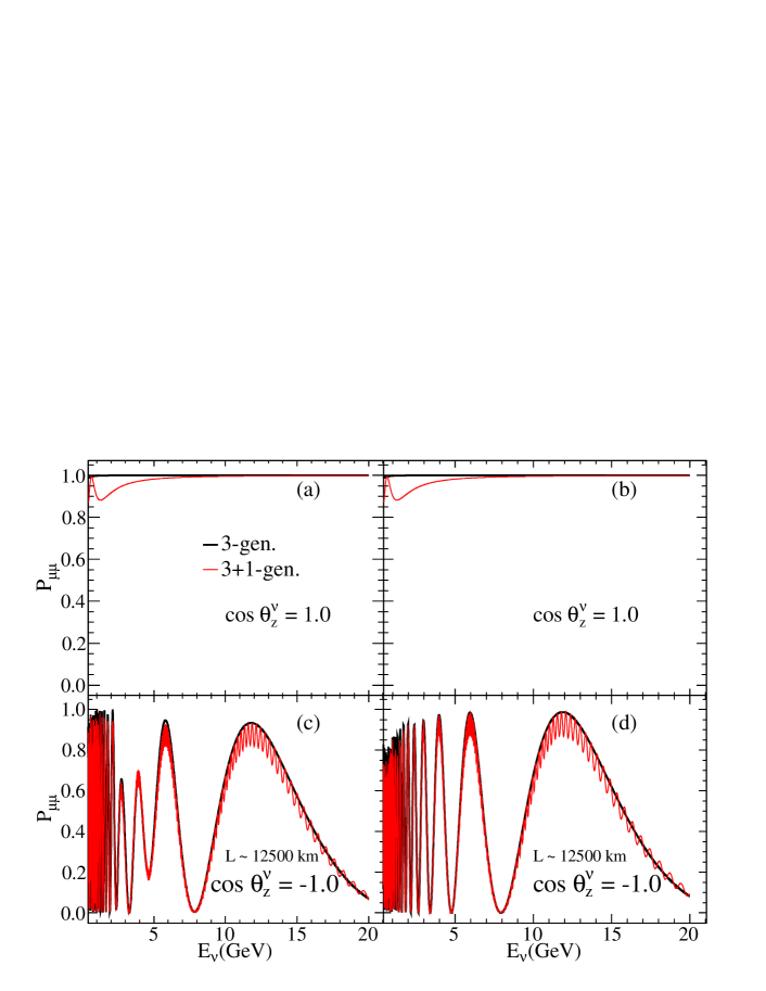
Figure 1: Comparison of the survival probability for neutrinos (left-hand panels) and anti-neutrinos (right-hand panels) for 3 (black line) and 3 $+$ 1 (red line) generations, as a function of (anti)neutrino energy. The top panels are for $\cos\theta^{\nu}_{z}=1.0$ (down-going neutrinos, L = 15 km) while the bottom panels are for $\cos\theta^{\nu}_{z}=-1.0$ (up-coming neutrinos, L = 12500 km). The oscillation parameters assumed for all panels are $\theta_{24}=10.0^{\circ}$ , $\theta_{14}=\theta_{34}=0.0^{\circ}$, $\Delta m^{2}_{41}=0.1$ eV², $\Delta m_{31}^{2}=2.4\times 10^{-3}$ eV², $\Delta m_{21}^{2}=7.5\times 10^{-5}$ eV², $\sin^{2}\theta_{23}=0.5$, $\sin^{2}\theta_{12}=0.3$, $\sin^{2}2\theta_{13}=0.1$ and all CP phases are taken as zero.

3.1 Matter effect on sterile neutrino oscillation

When atmospheric neutrinos travel through matter, they undergo coherent forward scattering on matter. The scattering is mediated by both charged and neutral current processes. The effective mass matrix in matter then changes to

$$M^{2}_{F}=UM^{(3~{}+~{}1)}U^{\dagger}+A\text{,}$$ (4)

where

$$M^{(3~{}+~{}1)}=diag(m^{2}_{1},m^{2}_{2},m^{2}_{3},m^{2}_{4}),$$ (5)

$$A=diag(A_{CC},0,0,A_{NC}),$$ (6)

where

$$A_{CC}=\pm 2\sqrt{2}G_{F}\rho N_{A}Y_{e}E\text{,}$$ (7)

and

$$A_{NC}=\pm\sqrt{2}G_{F}\rho N_{A}(1-Y_{e})E.$$ (8)

Here, $A_{CC}$ and $A_{NC}$ are the matter induced weak charged current (CC) and neutral current (NC) potentials, respectively, which depend on Fermi’s constant, $G_{F}$, matter density $\rho$, Avogadro number $N_{A}$, electron fraction $Y_{e}$ in matter and energy of neutrino $E$. In Eqs. (7) and (8), the “+” and “$-$” sign corresponds to neutrinos and antineutrinos, respectively. Only $\nu_{e}$ has CC interaction with electrons and NC interaction with electrons and nucleons, whereas $\nu_{\mu}$ and $\nu_{\tau}$ have only NC interaction and sterile neutrinos have no weak interactions. The analysis including matter effect has been carried out considering the varying density profile of the Earth $i.e.$ the preliminary reference Earth model (PREM) pre . Due to the matter effect, oscillation probability, as given in Eq. 3 will be modified, and in this work the neutrino oscillation probabilities are numerically calculated in matter for exact 3 $+$ 1 generation framework.

Figure 1 shows the survival probabilities for neutrinos (left-hand panels) and anti-neutrinos (right-hand panels) for 3 and 3 $+$ 1 generations, as a function of (anti)neutrino energy. The values of the parameters chosen to obtain the oscillation probabilities are given in the figure caption. The black and red lines show the plot for 3 and 3 $+$ 1 generation neutrinos, respectively considering the Earth matter effect. The top panels are for $\cos\theta^{\nu}_{z}=1.0$ (down-going neutrinos) while the bottom panels are for $\cos\theta^{\nu}_{z}=-1.0$ (upcoming neutrinos), where $\theta^{\nu}_{z}$ is the neutrino zenith angle. We show here the probabilities for the case when only the $\theta_{24}$ sterile mixing angle is taken as non-zero while $\theta_{14}=0=\theta_{34}$. The values of the other oscillation parameters are taken close to their current best-fit values and are given explicitly in the figure caption. The top panels show that while there is no oscillation of neutrinos for the standard 3 generation case whereas the 3 $+$ 1 generations show a small depletion which is same for neutrinos and antineutrinos. This is due to all CP phases being zero and oscillations happening in vacuum. The depletion which comes from active-sterile mixing can be used to constrain the sterile neutrino framework raj . The bottom panels show the presence of additional Earth matter effects due to active-sterile mixing. The rapid oscillation for 3 $+$ 1 generation neutrinos is due to the $|\Delta m^{2}_{41}|-$ driven phase factor of the oscillation probability. The ICAL detector is not expected to decipher these fast oscillations. For this $\cos\theta_{z}^{\nu}$ the neutrino and antineutrino survival probabilities have a difference coming mainly from $\Delta m_{31}^{2}-$ driven earth matter effects, while the impact due to sign of $\Delta m_{41}^{2}$ is hardly evident for this case where the mixing angles $\theta_{14}$ and $\theta_{34}$ are taken as zero.

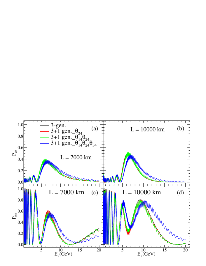
Figure 2: The neutrino oscillation probability P_eμ (top panels) and P_μμ (bottom panels) as a function of neutrino energy. The left-hand panels (right-hand panels) are for a neutrino trajectory corresponding to a baseline of $L=7000$ km ($L=10000$ km) inside earth. The black lines correspond to the 3 generation case, while the red, green, and blue lines correspond to the 3 $+$ 1 scenario. Specifically, the red lines are for $\sin^{2}\theta_{24}=0.03$, $\sin^{2}\theta_{14}=0$ and $\sin^{2}\theta_{34}=0$, the green lines are for $\sin^{2}\theta_{24}=0.03$, $\sin^{2}\theta_{14}=0.022$ and $\sin^{2}\theta_{34}=0$, while the blue lines are for $\sin^{2}\theta_{24}=0.03$, $\sin^{2}\theta_{14}=0.022$ and $\sin^{2}\theta_{34}=0.21$. The other oscillation parameters assumed for all panels are $\Delta m^{2}_{41}=1.0$ eV², $\Delta m_{31}^{2}=2.4\times 10^{-3}$ eV², $\Delta m_{21}^{2}=7.5\times 10^{-5}$ eV², sin${}^{2}\theta_{23}=0.5$, $\sin^{2}\theta_{12}=0.3$, $\sin^{2}2\theta_{13}=0.1$ and all CP phases are taken as zero.

Fig. 2 shows the appearance P_eμ (top panels) and survival, P_μμ (bottom panels), neutrino oscillation probabilities for 3 and 3 $+$ 1 generations, as a function of neutrino energy. The values of the mixing parameters chosen to obtain the oscillation probabilities are given in the figure caption. In particular, one can see that here we allow the sterile mixing angles $\theta_{14}$ and $\theta_{34}$ to be non-zero and study the impact of these on the oscillation probabilities. The left-hand panels have been obtained for a baseline of $L=7000$ km (corresponding to a zenith angle of $\cos\theta_{z}^{\nu}=-0.55$) and right-hand panels are for a baseline of $L=10000$ km (corresponding to a zenith angle of $\cos\theta_{z}^{\nu}=-0.785$). The black lines show the plot for the 3 generation case and red, green and blue lines represents for the 3 $+$ 1 generation neutrinos case. The red lines correspond to the case where only $\theta_{24}$ is taken as non-zero ($\sin^{2}\theta_{24}=0.03$ here). This is similar to the plots shown in Fig. 1. We next show in green lines the change obtained when we make $\theta_{14}$ non-zero. We notice a small difference between the red and green curves. Finally, in the blue lines we take all the 3 sterile mixing angles to be non-zero and their values are given in the figure caption. We see that the oscillations probabilities change significantly when $\theta_{34}$ is switched-on. Note that the oscillation probabilities P_eμ and P_μμ are independent of the value of $\theta_{34}$ as per the parametrization of the mixing matrix, and the effect of $\theta_{34}$ comes entirely due to earth matter effects Choubey:2007ji . Both the oscillation probabilities, P_eμ and P_μμ also show a shift in position of maxima or minima with inclusion of $\theta_{34}$. We notice from the figure that while each of the sterile mixing parameters changes the neutrino oscillation probabilities, the impact of $\theta_{34}$ appears to be most dramatic and changes the shape of the oscillation probabilities. It may be noted that, in this analysis both disappearance ($\nu_{\mu}\rightarrow\nu_{\mu}$) and appearance ($\nu_{e}\rightarrow\nu_{\mu}$) oscillation channels are considered while estimating the oscillated muon events for the atmospheric neutrinos.

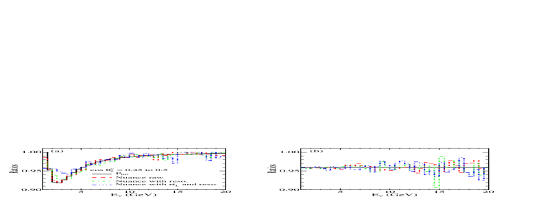
Figure 3: The ratio of oscillated to unoscillated events versus neutrino energy for the $\cos\theta_{z}$ bin 0.40 to 0.45. The active-sterile oscillation parameters are taken as $\theta_{14}=\theta_{34}=0$, $\sin^{2}2\theta_{24}=0.083$ and (a) $\Delta m^{2}_{41}$ = 0.1 eV², (b) $\Delta m^{2}_{41}$ = 10.0 eV². The black solid lines show the plot using the neutrino oscillation formula, the red dashed lines show the plot obtained using the NUANCE events without implementing the detector response, the green dot-dashed lines shows the plot using events after implementing the detector response of $\sigma_{E_{\nu}}$ = 0.15 E_ν and $\sigma_{\theta_{z}}$ = 10^∘, and the blue dashed-dotted lines show the plot for events after incorporating the detector response as well as the production height distribution of neutrinos given in Table I.

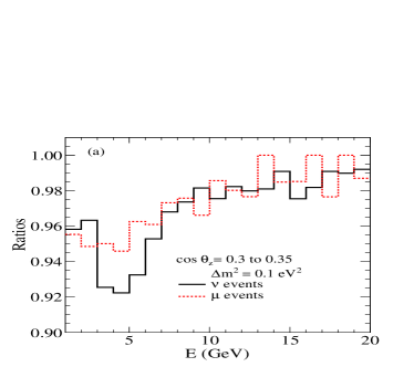
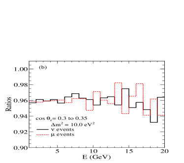
Figure 4: The ratio of oscillated to unoscillated events as a function of neutrino (black solid lines) and muon (red dashed lines) energy. The cos $\theta_{z}$ bin chosen is 0.30 to 0.35, $\theta_{14}=\theta_{34}=0$, $\sin^{2}2\theta_{24}=0.083$ and (a) $\Delta m^{2}_{41}$ = 0.1 eV², (b) $\Delta m^{2}_{41}$ = 10.0 eV². The standard oscillation parameters are same as in Fig. 3.

4 Simulation Technique

In this section we describe the simulation of atmospheric neutrino events in ICAL. The generation of the event spectrum and binning scheme are presented in subsection 4.1 and in subsection 4.2, respectively.

4.1 EVENT RECONSTRUCTION

The study on sterile neutrino sensitivity has been carried out using the detailed information of neutrino induced events. The atmospheric neutrinos, interacting with the iron target, produce leptons and hadrons through the charge current interaction. There are mainly three processes which contribute to the CC interactions in the ICAL detector. At the sub-GeV energy range, the quasi-elastic process dominates, in which the final state muon carries most of the available energy. As the energy increases from sub-GeV to multi-GeV, hadrons and their showers are produced in resonance (RS) and deep-inelastic scattering (DIS) processes. In the RS process, most of the hadron showers consist of a single pion, though multiple pions may contribute in a small fraction of events. On the other hand, in the DIS process multiple hadrons are produced which carry a large fraction of the incoming neutrino energy. In the CC interaction of neutrino, for every hadron shower, there is a corresponding muon coming from the same CC interaction vertex of neutrino.

Again, as shown in Fig. 1, the probability of active-sterile oscillations is valid only for down-going neutrinos, if one uses vacuum oscillations. However, the inclusion of the Earth matter effects for the upward going neutrino may contribute to the active-sterile oscillations. In what follows, we will consider neutrino events covering all zenith angles and present a comparison of the improvement coming from upcoming events.

The raw events without oscillations are generated using the NUANCE neutrino event generator modified for the ICAL detector. To reduce statistical fluctuations, initially data are generated for the 1000 years and further normalize to the required exposure during the statistical analysis. In this analysis, an exposure of 1 Mt-yr has been considered. Neutrino oscillations are then introduced through a re-weighting algorithm as discussed in Ghosh:2012px , which is based on the acceptance-rejection method. While calculating the neutrino oscillation probabilities, we consider the $\nu$ production height distribution in the atmosphere as a function of zenith angle and energy of neutrino which is given in TK for only downgoing neutrino. The path length (L) distribution was incorporated on MC basis by considering Gaussian smearing of the path length whose mean is L and the corresponding zenith angle and energy dependent sigma as given in Table I. It is to be noted that we have considered the production altitude distribution for down-going neutrinos only. This is because the sterile neutrino oscillations are relevant on small length scales and the uncertainty in the production point for the down-going neutrinos, therefore, becomes crucial.

Table 1: Production height (slant distance in km) of neutrinos and its corresponding sigma for six values of cos$\theta_{z}$ at three neutrino energy ranges TK

cos$\theta_{z}$	E = 0.3 $-$ 2.0 [GeV]		E = 2.0 $-$ 20.0 [GeV]		E $>$ 20.0 [GeV]
	L	$\sigma_{L}$	L	$\sigma_{L}$	L	$\sigma_{L}$
1.0	15.9	8.7	16.6	9.0	17.6	8.9
0.75	23.6	11.8	24.1	12.1	25.8	12.6
0.50	41.0	18.1	40.9	19.1	43.3	19.4
0.25	95.6	31.4	92.8	34.6	94.9	36.4
0.15	160.0	37.3	154.3	42.8	151.2	49.4
0.05	369.8	55.0	359.0	67.1	335.7	94.2

Figure 3 shows the ratio of events with and without oscillations taken into account as a function of neutrino energy. The results are shown for the neutrinos and a particular zenith angle bin of $\cos\theta_{z}^{\nu}=0.45-0.5$. Fig. 3(a) is for $\Delta m_{41}^{2}=0.1$ eV² while Fig. 3(b) is for $\Delta m_{41}^{2}=10.0$ eV². The black lines show the survival probability $P_{\mu\mu}$ as a function of the neutrino energy. The red line shows the ratio of raw events from NUANCE with and without oscillations. Note that the red lines follow the survival probability fairly close, within the MC fluctuation. The green lines are obtained by including a flat energy and angle resolution for the neutrino events. We assume a flat resolution of $\sigma_{E_{\nu}}$ = 0.15 $E_{\nu}$ and $\sigma_{\theta_{z}^{\nu}}$ = $10^{\circ}$ in this illustrative figure. It may be noted that, the energy and the zenith angle correspond to true values obtained from the NUANCE output. On the other hand, the reconstructed energy and zenith angle correspond to the neutrino events after incorporating detector resolutions. The resolution functions bring a mild smearing of the shape of the event spectrum. Finally, the blue lines are obtained after smearing for the production point in the atmosphere as well according to Table 1. The impact of this smearing is rather large when the data is sensitive to the phase of the $\Delta m_{41}^{2}$ driven oscillations (left panel). Since the production point becomes uncertain, the path length becomes uncertain, causing a drop in the effective dip of the event spectrum due to active sterile oscillations.

The ICAL simulations are performed not in terms of the neutrino energy and angle, but in terms of muon energy and angle and hadron energies. Hence the oscillated events are distributed two dimensionally in terms of final state muon energy and muon zenith angle bins. The hadron events are binned in hadron energy only. The detector energy resolution, angle resolution, charge and reconstruction efficiencies are next incorporated in the simulations. We have incorporated the actual resolutions of the detector for muons and hadrons using INO look up tables ac ; mo . The muon energy and zenith angle resolutions are a function of both energy as well as zenith angle. To incorporate the detector response in the true event distribution numerically, we have used the Monte Carlo (MC) methods. At low energy (E $<$ 0.9 GeV), the energy loss of muons in the detector follow a Landau probability distribution function (p.d.f) and above this a Gaussian p.d.f. For a particular event, the Landau p.d.f (P_L) for E_μ $<$ 0.9 GeV and Gaussian p.d.f. (P_G) above 0.9 GeV have been used to smear the true energy of muon. To incorporate the energy dependent zenith angle resolution of muon, the P_G has been used for all energy. The mean of the function are true $E_{\mu}$, cos $\theta_{z}$ for energy and zenith angle of muons, respectively, without incorporating the ICAL detector resolutions. The final energy and cosine of zenith angles are as follows,

$$E^{r}_{\mu}=P_{L}(E_{\mu},\,\,\sigma_{E_{\mu}}),E<\,\text{0}.9\,GeV$$ (9)

$$E^{r}_{\mu}=P_{G}(E_{\mu},\,\,\sigma_{E_{\mu}}),E\geq\,\text{0}.9\,GeV$$ (10)

$$cos^{r}\theta_{z}=P_{G}(cos\ \theta_{z},\sigma_{cos\theta_{z}})$$ (11)

where $\sigma$${}_{E_{\mu}}$ is the standard deviation of energy, $\sigma$${}_{cos{\theta_{z}}}$ is the standard deviation for cosine of zenith angle taken from ac , and $E^{r}_{\mu}$, $cos^{r}\theta_{z}$ are reconstructed energy and cosine of zenith angle of muons, respectively. To incorporate the hadron energy resolutions in the ICAL simulation, the Vavilov probability distribution function has been used as described in mo .

In Fig. 4 the red dashed lines show the ratio of events, with and without oscillations, binned in muon energy and in the muon zenith angle range $\cos\theta_{z}$ = 0.3 to 0.35. For comparison we also show in the black solid lines the ratio of events, with and without oscillations, binned in terms of neutrino energies and in the neutrino zenith angle range of $\cos\theta_{z}^{\nu}$ = 0.3 to 0.35. The left panel (a) is for $\Delta m_{41}^{2}=0.1$ eV² while the right panel (b) is for $\Delta m_{41}^{2}=10.0$ eV². The number of downgoing without oscillated events are 12984 and oscillated events are 11868 for an exposure of 1 MTon-year. The expected rate of neutrinos assuming no sterile neutrinos as a function of cosine of zenith angle (cos$\theta_{z})$ and energy (E_μ is shown in Fig. 5(a). The relative reduction in expected neutrinos events rate for the mixing parameters around the best fit Kopp:2013vaa is shown in Fig. 5(b). It may be noted here that the events distribution are obtained after incorporating the detector resolution as well as detector reconstruction efficiencies.

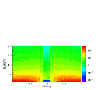
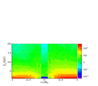
Figure 5: (a) Without oscillated event distribution (b) Oscillated event distributions.

4.2 Binning scheme

After incorporating the ICAL detector resolutions for muons and hadrons in neutrino induced events, a variable binning scheme has been adopted to study the sensitivity of sterile neutrinos oscillation. In a simulation the bin content may be less than one, but in an experiment, the observed data in various bins should be greater than or equal to one. The bins of different widths are chosen in order to ensure that there is at least one event in each bin. The binning schemes for down-going neutrinos induced events are given in Table 2 and 3. Table 2 gives the binning scheme for the down-going events using only the muon energy and zenith angle. Table 3 on the other hand gives the binning scheme for the analysis with the down-going events where the hadron energy information is used in addition to muon energy and zenith angle. Since the muon reconstruction efficiency is nearly zero for near-horizontal bin, we set a lower limit of $\cos\theta_{z}>0.1$. The production of atmospheric neutrino flux follows a steep power law in energy($\sim$ E^-2.7), resulting in a smaller number of events at higher muon and hadron energies. Therefore, finer bins at low energies and wider bins at higher energies are considered for both muons and hadrons, respectively. Moreover, it may be noticed that at low energies ($E=1-1.5$ GeV) and high zenith angle ($\cos\theta_{z}=0.1-0.2$), a larger bin width is considered due to the fact that the reconstruction efficiency of ICAL is poor in this region.

Similar arguments were adopted in choosing the binning scheme when considering events due to neutrinos coming from all directions. The details on the bin combinations for the cases when only muon energy and its zenith angle are used and when hadron energy information is used as well, are given in Tables 4 and 5 respectively. It is to be noted that wider bin combinations are considered for upcoming neutrinos induced events due to the further depletion of events as a result of oscillation of neutrinos in these cases.

Table 2: The binning scheme adopted for the reconstructed parameters E_μ and cos $\theta_{z}$ for muons induced due to downgoing neutrinos, where $\chi^{2}$ is estimated considering only muon events.

Parameter	Range	Bin width	Total bins
E$\mu$(GeV)	[1, 1.5]	0.5	1
	[1.5, 3.0]	0.25	6
	[3, 11]	0.5	16
	[11, 16]	1	5
	[16, 20]	2	2
cos $\theta_{z}$	[0.1, 0.2]	0.05	2
	[0.2, 1.0]	0.025	32

Table 3: The binning scheme adopted for the reconstructed parameters E_μ, cos $\theta_{z}$ and E_h for muons and hadrons, respectively, where $\chi^{2}$ is estimated considering combined muon and hadron information of downgoing neutrino induced events.

Parameter	Range	Bin width	Total bins
E$\mu$(GeV)	[1, 1.5]	0.5	1
	[1.5, 5.5]	0.25	16
	[5.5, 8]	0.5	7
	[8, 13]	1	5
	[13, 17]	2	2
	[17, 20]	3	1
cos $\theta_{z}$	[0.1, 0.25]	0.15	1
	[0.25, 1.0]	0.05	15
Eh	[0, 3]	3	1
	[3, 20]	17	1

Table 4: The binning scheme adopted for the reconstructed parameters E_μ and cos $\theta_{z}$ for muons produced due to both upcoming and downgoing neutrinos, for the $\chi^{2}$ estimations with muons only.

Parameter	Range	Bin width	Total bins
E$\mu$(GeV)	[1, 1.5]	0.5	1
	[1.5, 3.0]	0.25	6
	[3.0, 6.0]	0.5	6
	[6, 11]	1.0	5
	[11, 13]	2	1
	[13, 16]	3	1
	[16, 20]	4	1
cos $\theta_{z}$	[-1.0, -0.3]	0.025	28
	[-0.3, 0.1]	0.4	1
	[0.1, 0.2]	0.1	1
	[0.2, 1.0]	0.025	32

Table 5: The binning scheme adopted for the reconstructed parameters E_μ, cos $\theta_{z}$ and E_h for muons and hadrons where $\chi^{2}$ is estimated considering combined muon and hadron information and for the upcoming and downgoing neutrino induced events.

Parameter	Range	Bin width	Total bins
E$\mu$(GeV)	[1, 2]	1.0	1
	[2, 7]	0.5	10
	[7, 10]	1.0	3
	[10, 12]	2	1
	[12, 15]	3	1
	[15, 20]	5	1
cos $\theta_{z}$	[-1.0, -0.3]	0.1	7
	[-0.3, 0.1]	0.4	1
	[0.1, 0.3]	0.1	2
	[0.3, 1.0]	0.05	14
Eh	[0, 2]	2	1
	[2, 20]	18	1

5 $\chi^{2}$ ESTIMATION

To incorporate the muon energy and angle information in the analysis, we define a $\chi^{2}$ as pu

$$\begin{split}\chi^{2}_{muons}=\ &\min_{\xi_{i}}\sum_{n_{1}=0}^{N_{1}}\sum_{n_{2}=0}^{N_{2}}\left[2\left(R_{n_{1},n_{2}}^{th}-R_{n_{1},n_{2}}^{ex}\right)\right.\\ &\left.+2R_{n_{1},n_{2}}^{ex}\,\ln\left(\frac{R_{n_{1},n_{2}}^{ex}}{R_{n_{1},n_{2}}^{th}}\right)\right]+\sum_{i=0}^{k}\xi_{i}^{2}\end{split}$$ (12)

and

$$R_{n_{1},n_{2}}^{th}=R_{n_{1},n_{2}}^{{}^{\prime}th}\left(1+\sum_{i=0}^{k}\pi_{n_{1}n_{2}}^{i}\xi_{i}\right)+\mathcal{O}(\xi^{2})$$ (13)

where $n_{1}$ and $n_{2}$ are number of bins for energy and cosine of the zenith angle for muons, $R_{n_{1},n_{2}}^{ex}$, $R_{n_{1},n_{2}}^{{}^{\prime}th}$ are observed and theoretically predicted events, $\pi_{n}^{i}$ is the strength of the coupling between the pull variable $\xi_{i}$ and $R_{n_{1},n_{2}}^{th}$ which carries the information about systematic uncertainties as given in Eq. (13). Equation (12) is minimized with respect to pull variables. Five systematic uncertainties, $viz.$ an overall flux normalization error of 20$\%$ , overall normalization of cross-section of 10$\%$, flux tilt factor of 5$\%$ which takes into account the deviation of the atmospheric fluxes from a power law, zenith angle dependence of the flux of 5$\%$ and finally an overall 5$\%$ systematic error are considered. More discussion on implementation of systematic uncertainty can be found in Ref. Ghosh:2012px . The information on the hadron energy is incorporated along with the muon energy and angle information by defining the $\chi^{2}$ as

$$\begin{split}\chi^{2}_{muons+hadrons}=\ &\min_{\xi_{i}}\sum_{n_{1}=0}^{N_{1}}\sum_{n_{2}=0}^{N_{2}}\sum_{n_{3}=0}^{N_{3}}\left[2\left(R_{n_{1},n_{2},n_{3}}^{th}-\right.\right.\\ \left.R_{n_{1},n_{2},n_{3}}^{ex}\right)\\ &\left.+2R_{n_{1},n_{2},n_{3}}^{ex}\,ln\left(\frac{R_{n_{1},n_{2},n_{3}}^{ex}}{R_{n_{1},n_{2},n_{3}}^{th}}\right)\right]+\sum_{i=0}^{k}\xi_{i}^{2}\end{split}$$ (14)

where the index $n_{3}$ runs over the hadron energy bins. The other variables are the same as defined before. It may be noted that the theoretically predicted and observed events correspond to with and without sterile neutrino oscillated events, respectively.

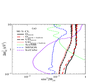
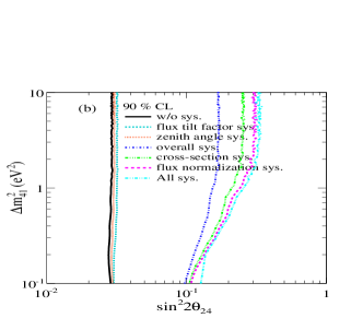
Figure 6: (a)The 90% C.L. exclusion limits in the $\Delta m_{41}^{2}-\sin^{2}2\theta_{24}$ plane, where $\sin^{2}2\theta_{24}=4U^{2}_{\mu 4}(1-U_{\mu 4})^{2}$, expected from 1 Mt-yr of the ICAL data. The legends ‘D’ and ‘UD’ correspond to only downward-going neutrinos and neutrinos from all directions. Here, the other active-sterile mixing angles are taken as $\theta_{14}$ = $\theta_{34}$ = 0.0^∘. The 90% C.L. SciBooNE/MiniBooNE, MINOS and IceCube exclusion regions are shown for comparison, (b) impact of individual systematic uncertainty on the sensitive limits.

The $\chi^{2}$ so defined is next marginalized over the sterile neutrino oscillation parameters $\Delta m_{41}^{2}$ and the mixing angles $\theta_{14}$, $\theta_{24}$ and $\theta_{34}$. The total $\chi^{2}$, is estimated by adding the priors of $\Delta m_{41}^{2}$ and $\theta_{14}$, $\theta_{24}$ and $\theta_{34}$,

$$\begin{split}\chi^{2}_{total}=\ &\chi^{2}+\left(\frac{(\Delta m^{2}_{41})^{bf}-\Delta m^{2}_{41})}{\sigma(\Delta m^{2}_{41})}\right)^{2}\\ &+\left(\frac{(\sin^{2}(2\theta_{ij})^{bf}-\sin^{2}(2\theta_{ij})}{\sigma(\sin^{2}(2\theta_{ij})}\right)^{2}\end{split}$$ (15)

The parameters sin${}^{2}2\theta_{ij}$ and $\Delta m^{2}_{41}$ are varied within the range of 0.047 to 0.22 and 0.82 eV² to 2.19 eV², respectively. The error on sin${}^{2}2\theta_{ij}$ and $\Delta m^{2}_{41}$ are considered as 10$\%$ of their assumed true values.

6 EXCLUSION LIMITS

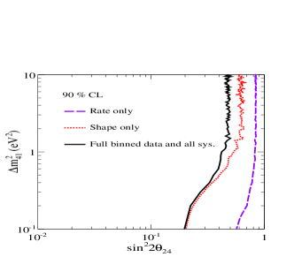
Figure 7: Comparisons of exclusion limits in the $\Delta m_{41}^{2}$ - $\sin^{2}2\theta_{24}$ plane for rate-only, shape-only and including all systematics with consideration of downgoing neutrinos only.

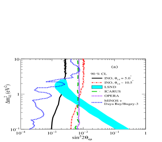
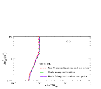
Figure 8: (a)The 90% exclusion limits in the $\Delta m_{41}^{2}$ - $\sin^{2}2\theta_{e\mu}$ plane where sin${}^{2}2\theta_{e\mu}$= 4 $U^{2}_{e4}U_{\mu 4}^{2}$, expected from an exposure of 1 Mt-yr of the ICAL data. The active-sterile mixing angles are considered fixed at $\theta_{14}=5.0^{\circ}$ and 10.5^∘ and $\theta_{34}$ = 0.0^∘. The 90% C.L. allowed regions from the LSND and the 90% C.L. excluded regions of OPERA, ICARUS and the combined results from MINOS and Daya Bay/Bugey-3 experiments are shown for comparisons, (b) effect of marginalization over $\theta_{14}$ with its 1$\sigma$ range.

The oscillation probabilities of atmospheric neutrinos depend on the active-sterile neutrino mixing. The data from ICAL will therefore be sensitive to this mixing and should be able to constrain them. The upper limit for the sterile neutrino mixing angle $\theta_{24}$ for an exposure of 1Mt-yr is shown in Fig. 6. For simplicity we take the mixing angles $\theta_{14}$ and $\theta_{34}$ to be zero in this plot. The black lines correspond to the sensitivity obtained in the analysis when only muon energy and angle information is used, while the red lines correspond to the expected sensitivity when the hadron energy together with muon energy and angle information are included as well. A comparison of the black and red lines shows that the addition of hadron energy information in the analysis does not bring any significant improvement in the sensitivity. We show the expected sensitivity for the case where only down-going neutrinos are considered as well as when data from all zenith angles are analyzed. The lines labeled as ‘D’ in the figure show the expected exclusion plots where only down-going events are considered, while the lines labeled as ‘UD’ in the figure show the expected sensitivity when neutrino events from all zenith angles are included in the analysis. The inclusion of up-going neutrinos is seen to improve the sensitivity to the sterile mixing angle $\theta_{24}$. The improvement comes from the increase of statistics as well as from the inclusion of earth matter effects which change with the inclusion of active-sterile mixing. With 1 Mt-yr data, ICAL is expected to limit $\sin^{2}2\theta_{24}<0.19$ at the 90% C.L. for $\Delta m_{41}^{2}\sim 0.1$ eV² using the down-going events only. This limit is expected to improve to $\sin^{2}2\theta_{24}<0.12$ when events from all zenith angles are included. This constitutes an improvement of about 35$\%$.

We also show in Fig. 6(a), the exclusion plots from other experiments for comparison. The green dashed dotted line in Fig. 6(a) shows the exclusion plot from the SciBooNE/MiniBooNE mb experiment which looked for $\nu_{\mu}$ disappearance. It is found that at lower values of $\Delta m^{2}_{41}$, the ICAL detector has better sensitivity compared to SciBooNE/ MiniBooNE due to the longer path length and lower energies of the atmospheric neutrinos. The blue dashed double-dotted line shows results from the MINOS Sousa:2015bxa experiment for comparisons which corresponds to disappearance search of the $\nu_{\mu}$, in the range of $\Delta m^{2}_{43}$ = 0.1-10 eV² while their results spans over $\Delta m^{2}_{43}$ = 0.01-100 eV². In addition the violet line shows the result from IceCube TheIceCube:2016oqi . Figure 6(b) shows the impact of individual systematics on the active-sterile mixing sensitivity. It is found that the uncertainty due to flux normalization has the maximum effect compared to the others. In addition the exclusion limits are obtained performing the rate only analysis considering single bin in energy and keeping the zenith angle bins same as given in Table 2 and also shape only analysis by removing the pull term on neutrino flux from the chi-square function where we consider the downgoing neutrinos only. Figure 7 shows the comparison of exclusion limits obtained from shape only (red dashed line) and the rate only (violet line) analysis at 90% C.L. The lower limit on $\sin^{2}2\theta_{24}\sim$ 0.57 at $\Delta m^{2}_{41}$ = 0.1 eV² obtained from the rate only analysis. However, while doing the rate only analysis by merging all the angle and energy bins, the limit on $\sin^{2}2\theta_{24}\sim$ 0.70 at $\Delta m^{2}_{41}$ = 0.1 eV² at 68 $\%$ C.L. It has been observed that the exclusion limits from shape only analysis ($\sin^{2}2\theta_{24}\sim$ 0.59) is less sensitive compare to the results obtained from the analysis of full binned data and including the pull corresponding to all systematic errors ($\sin^{2}2\theta_{24}\sim$ 0.47) at higher values of $\Delta m^{2}_{41}$ = 10.0 eV². However, at low value of $\Delta m^{2}_{41}$ = 0.1 eV² the difference is $\sim$ 3 $\%$.

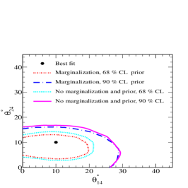
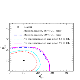
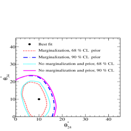
Figure 9: The expected allowed areas in the $\theta_{14}-\theta_{24}$ plane (left-hand panel), $\theta_{14}-\theta_{34}$ plane (middle panel), and $\theta_{24}-\theta_{34}$ plane (right-hand panel), expected from 1 Mt-yr of ICAL data. The standard 3-generation oscillation parameters are taken as sin${}^{2}\theta_{12}=0.3$, sin${}^{2}2\theta_{13}=0.1$, sin${}^{2}\theta_{23}=0.5$ , $\Delta m^{2}_{21}$ = 7.5 $\times$ 10^-5 eV² , $\Delta m^{2}_{31}$ = 2.4 $\times$ 10^-3 eV². The data is generated at $\theta_{14}=\theta_{24}=\theta_{34}=10^{\circ}$ and at $\Delta m^{2}_{41}=1$ eV². We marginalize the $\chi^{2}$ over $\Delta m^{2}_{41}$ and the remaining sterile mixing angle, viz., $\theta_{34}$ in the left-hand panel, $\theta_{24}$ in the middle panel and $\theta_{14}$ in the right-hand panel. The priors considered are described in Sec. 5.

Figure 8(a) shows the expected sensitivity of ICAL to the effective mixing angle $\theta_{e\mu}$ which for the active-sterile mixing case is defined as $\sin^{2}2\theta_{e\mu}=4U^{2}_{e4}U_{\mu 4}^{2}$. We have taken a statistics corresponding to 1 Mt-yr data at ICAL and considered the information on just the muon energy and zenith angles. We show the 90% C.L. expected exclusion limits in the $\Delta m^{2}_{41}-\sin^{2}2\theta_{e\mu}$ plane for fixed choices of $\theta_{14}\sim 5.0^{\circ}$ (solid black line) and $10.5^{\circ}$ (dashed double-dotted red line). For both these case we keep $\theta_{34}=0.0^{\circ}$. The cyan shaded region shows the 90% C.L. allowed region from the LSND Aguilar:2001ty experiment for comparison. The green long-dashed line shows the results from the ICARUS Antonello:2013gut while the purple dotted line shows the results OPERA Agafonova:2013xsk . The sensitivity of the ICAL experiment is seen to increase significantly depending on the value of $\theta_{14}$ and could in principle rule out significant parts of the LSND allowed region. The blue dashed line shows results obtained from combined analysis of MINOS and Daya Bay/Bugey-3 experimental data at 90% C.L Adamson:2016jku . Figure 8(b) shows the marginalization effect of $\theta_{14}$ on the sensitivity $\sin^{2}2\theta_{e\mu}$. The 1$\sigma$ range of $\theta_{14}$ was considered from Ref. Giunti:2013waa . It is observed that the impact on $\sin^{2}2\theta_{e\mu}$ is negligible. Further exclusion plots are generated for various mixing angle combinations considering only muon energies and zenith angles and shown in Fig. 9. The data for these figures are generated for assumed true values of sterile mixing angles of $\theta_{14}=\theta_{24}=\theta_{34}=10^{\circ}$ and at $\Delta m^{2}_{41}$ = 1 eV². The assumed true values of the standard oscillation parameters are given in the figure caption. Figure 9 shows the expected constraints from 1 Mt$-$yr of ICAL data in the $\theta_{14}-\theta_{24}$ plane in the left-hand panel, $\theta_{14}-\theta_{34}$ plane in the middle-panel, and $\theta_{24}-\theta_{34}$ plane in the right-hand panel. The point at which the data is generated is shown by the black dots. The different lines show the different marginalizing methods, with added priors and at different C.L., and the details are given in the figure legends. For the cases which include marginalization, we have marginalized the $\chi^{2}$ over $\Delta m^{2}_{41}$ and the remaining sterile mixing angle, viz., $\theta_{34}$ in the left-hand panel, $\theta_{24}$ in the middle panel and $\theta_{14}$ in the right-hand panel, with priors, as was discussed in the previous section. For the case with marginalization, we expect an upper bound at 90% C.L. (from 2 parameter plots) of around $20^{\circ}$ for $\theta_{14}$ and $\theta_{34}$, and about $12^{\circ}$ for $\theta_{24}$. On the lower side only $\theta_{24}$ is seen to be bounded at 90% C.L. without priors and at 68% C.L. once priors are included. While for both the other mixing angles, the cases $\theta_{14}=0$ and $\theta_{34}=0$ are expected to be compatible with the data at even the $1\sigma$ C.L. for all analyses that we considered.

7 SUMMARY

The sensitivity of ICAL to active-sterile neutrino mixing is studied. The effect of inclusion of hadron energy into the analysis has been probed. The present analysis shows that the inclusion of upcoming neutrinos, which are affected by the intervening matter, improves the sensitivity to sterile neutrino mixing. The inclusion of hadron energy information in the analysis, on the other hand, has almost no effect on the sensitivity to sterile neutrino mixing. From the down-going events alone, one expects an upper bound of $\sin^{2}2\theta_{24}<0.16$ at 90% C.L. from 1 Mt-yr of data. The sensitivity to the sterile neutrino mixing angle further improves by considering neutrinos coming from all directions at the detector. There is enhancement in sensitivity by about 35$\%$ for the whole range of $\Delta m^{2}_{41}$. At lower values of $\Delta m^{2}_{41}$, the ICAL detector has better sensitivity compared to the short baseline experiments like SciBooNE/MiniBooNE. Also expected bounds on the sterile mixing angles are obtained. For an illustrative case of assumed true value of $10^{\circ}$ for all the three sterile mixing angles and after marginalization, an upper bound at 90% C.L. (from 2 parameter plots) of around $20^{\circ}$ for $\theta_{14}$ and $\theta_{34}$, and about $12^{\circ}$ for $\theta_{24}$ is obtained. The impact of inclusion of priors on the sterile neutrino parameters is studied. Only for $\theta_{24}$ could one rule out the zero-mixing possibility at 90% C.L. for this illustrative case, while for both the other mixing angles $\theta_{14}=0$ and $\theta_{34}=0$ are compatible with the data at even the $1\sigma$ C.L..

References

- (1) B. T. Cleveland, T. Daily, R. Davis, Jr., J. R. Distel, K. Lande, C. K. Lee, P. S. Wildenhain and J. Ullman, Astrophys. J. 496, 505 (1998); M. Altmann et al. [GNO Collaboration], Phys. Lett. B 616, 174 (2005); J. Hosaka et al. [Super-Kamiokande Collaboration], Phys. Rev. D 73, 112001 (2006); Q. R. Ahmad et al. [SNO Collaboration], Phys. Rev. Lett. 89, 011301 (2002); B. Aharmim et al. [SNO Collaboration], Phys. Rev. Lett. 101, 111301 (2008); B. Aharmim et al. [SNO Collaboration], Phys. Rev. C 81, 055504 (2010); C. Arpesella et al. [Borexino Collaboration], Phys. Rev. Lett. 101, 091302 (2008).
- (2) Y. Fukuda et al. [Super-Kamiokande Collaboration], Phys. Rev. Lett. 81, 1562 (1998); Y. Ashie et al. [Super-Kamiokande Collaboration], Phys. Rev. D 71, 112005 (2005); R. Wendell et al., [Super-Kamiokande Collaboration], Phys. Rev. D,81,092004 (2010).
- (3) T. Araki et al. [KamLAND Collaboration], Phys. Rev. Lett. 94, 081801 (2005); S. Abe et al. [KamLAND Collaboration], Phys. Rev. Lett. 100, 221803 (2008).
- (4) F. P. An et al. [Daya Bay Collaboration], Phys. Rev. Lett. 108, 171803 (2012); F. P. An et al. [Daya Bay Collaboration], Chin. Phys. C 37, 011001 (2013).
- (5) J. K. Ahn et al. [RENO Collaboration], Phys. Rev. Lett. 108, 191802 (2012).
- (6) Y. Abe et al. [Double Chooz Collaboration],TWO Phys. Rev. Lett. 108, 131801 (2012); Y. Abe et al. [Double Chooz Collaboration], Phys. Rev. D 86, 052008 (2012).
- (7) M. H. Ahn et al. [K2K Collaboration], Phys. Rev. D 74, 072003 (2006).
- (8) P. Adamson et al. [MINOS Collaboration], Phys. Rev. Lett. 101, 131802 (2008); P. Adamson et al. [MINOS Collaboration], Phys. Rev. Lett. 107, 181802 (2011); P. Adamson et al. [MINOS Collaboration], Phys. Rev. Lett. 110, 171801 (2013).
- (9) K. Abe et al. [T2K Collaboration], Phys. Rev. Lett. 107, 041801 (2011); K. Abe et al. [T2K Collaboration], Phys. Rev. D 88, 032002 (2013).
- (10) M. C. Gonzalez-Garcia, M. Maltoni, J. Salvado and T. Schwetz, JHEP 1212, 123 (2012).
- (11) A. Aguilar-Arevalo et al. [LSND Collaboration], Phys. Rev. D 64, 112007 (2001).
- (12) E. Akhmedov and T. Schwetz, JHEP 1010, 115 (2010).
- (13) C. Giunti and M. Laveder, Phys. Rev. D 84, 073008 (2011).
- (14) G. Karagiorgi, Z. Djurcic, J. M. Conrad, M. H. Shaevitz and M. Sorel, Phys. Rev. D 80, 073001 (2009) Erratum: [Phys. Rev. D 81, 039902 (2010)].
- (15) J. Beringer et al. [Particle Data Group Collaboration], Phys. Rev. D 86, 010001 (2012).
- (16) B. Armbruster et al. [KARMEN Collaboration], Phys. Rev. D 65, 112001 (2002).
- (17) A. A. Aguilar-Arevalo et al. [MiniBooNE Collaboration], Phys. Rev. Lett. 105, 181801 (2010).
- (18) A. A. Aguilar-Arevalo et al. [MiniBooNE Collaboration], Phys. Rev. Lett. 110, 161801 (2013).
- (19) G. Mention, M. Fechner, T. Lasserre, T. A. Mueller, D. Lhuillier, M. Cribier and A. Letourneau, Phys. Rev. D 83, 073006 (2011).
- (20) P. Huber, Phys. Rev. C 85, 029901 (2012).
- (21) A. C. Hayes, J. L. Friar, G. T. Garvey, G. Jungman and G. Jonkmans, Phys. Rev. Lett. 112, 202501 (2014).
- (22) D. A. Dwyer and T. J. Langford, Phys. Rev. Lett. 114, 012502 (2015).
- (23) M. A. Acero, C. Giunti and M. Laveder, Phys. Rev. D 78, 073009 (2008).
- (24) C. Giunti and M. Laveder, Phys. Rev. C 83, 065504 (2011).
- (25) V. Gavrin, B. Cleveland, S. Danshin, S. Elliott, V. Gorbachev, T. Ibragimova, A. Kalikhov and T. Knodel et al., Phys. Part. Nucl. 46, 131 (2015).
- (26) T. Lasserre, Nucl. Phys. Proc. Suppl. 235-236, 214 (2013).
- (27) P. A. R. Ade et al. [Planck Collaboration], Astron. Astrophys. 566, A54 (2014).
- (28) R. Gandhi and P. Ghoshal, Phys. Rev. D 86, 037301 (2012).
- (29) D. Casper, nuint.ps.uci.edu/nuance/default.htm.
- (30) A. Chatterjee, K. K. Meghna, K. Rawat, T. Thakore, V. Bhatnagar, R. Gandhi, D. Indumathi and N. K. Mondal et al., JINST 9, P07001 (2014).
- (31) M. M. Devi, A. Ghosh, D. Kaur, L. S. Mohan, S. Choubey, A. Dighe, D. Indumathi and S. Kumar et al., JINST 8, P11003 (2013).
- (32) G. Majumder, N. K. Mondal, S. Pal, D. Samuel, and B. Satyanarayana, Nucl. Instrum. Meth. 735, 88 (2014).
- (33) S. P. Behera, M. S. Bhatia, V. M. Datar and A. K. Mohanty, IEEE Trans. Magn., 51, 1 (2015).
- (34) M. M. Devi, T. Thakore, S. K. Agarwalla and A. Dighe, JHEP 1410, 189 (2014).
- (35) D. Kaur, M. Naimuddin and S. Kumar, Eur. Phys. J. C 75, 156 (2015).
- (36) T. Thakore, A. Ghosh, S. Choubey and A. Dighe, JHEP 1305, 058 (2013).
- (37) A. Ghosh and S. Choubey, JHEP 1310, 174 (2013).
- (38) A. Chatterjee, R. Gandhi and J. Singh, JHEP 1406, 045 (2014).
- (39) M. Maltoni and T. Schwetz, Phys. Rev. D 76, 093005 (2007).
- (40) J. Kopp, P. A. N. Machado, M. Maltoni and T. Schwetz, JHEP 1305, 050 (2013).
- (41) A. M. Dziewonski and D. L. Anderson, Phys. Earth Planet. Inter. 25, 297 (1981).
- (42) S. Choubey, JHEP 0712, 014 (2007).
- (43) A. Ghosh, T. Thakore and S. Choubey, JHEP 1304, 009 (2013).
- (44) T. K. Gaisser and T. Stanev, Phys. Rev. D 57, 1977 (1998).
- (45) M. C. Gonzalez-Garcia and M. Maltoni, Phys. Rev. D 70, 033010 (2004).
- (46) K. B. M. Mahn et al. [SciBooNE and MiniBooNE Collaborations], Phys. Rev. D 85, 032007 (2012).
- (47) A. B. Sousa [MINOS and MINOS+ Collaborations], AIP Conf. Proc. 1666, 110004 (2015).
- (48) M. G. Aartsen et al. [IceCube Collaboration], Phys. Rev. Lett. 117, 071801 (2016).
- (49) M. Antonello et al. [ICARUS Collaboration], Eur. Phys. J. C 73, 2599 (2013).
- (50) N. Agafonova et al. [OPERA Collaboration], JHEP 1307, 004 (2013); JHEP 1307, 085 (2013).
- (51) P. Adamson et al. [Daya Bay and MINOS Collaborations], Phys. Rev. Lett. 117, 151801 (2016).
- (52) C. Giunti, arXiv:1311.1335 [hep-ph].