Wehrl entropies and Euclidean Landau levels

Abstract.

We are concerned with an information-theoretic measure of uncertainty for quantum systems. Precisely, the Wehrl entropy of the phase-space probability $Q^{(m)}_{\hat{\rho}}=\left\langle z,m|\hat{\rho}|z,m\right\rangle$ which is known as Husimi function, where $\hat{\rho}$ is a density operator and $\left|z,m\right\rangle$ are coherent states attached to an Euclidean $m$th Landau level. We obtain the Husimi function $Q^{(m)}_{\beta}$ of the thermal density operator $\hat{\rho}_{\beta}$ of the harmonic oscillator, which leads by duality, to the Laguerre probability distribution of the mixed light. We discuss some basic properties of $Q^{(m)}_{\beta}$ such as its characteristic function and its limiting logarithmic moment generating function from which we derive the rate function of the sequence of probability distributions $Q^{(m)}_{\beta},\ m=0,1,2,...$. For $m\geq 1$, we establish an exact expression for the Wehrl entropy of the density operator $\hat{\rho}_{\beta}$ and we discuss the behavior of this entropy with respect to the temperature parameter $T=1/\beta$.

1. Introduction

A coherent state $\left|\alpha\right\rangle$, $\alpha\in X$, is a specific overcomplete family of normalized vectors in a Hilbert space $\mathcal{H}$ corresponding to quantum phenomena and provide $\mathcal{H}$ with the following resolution of identity

(1.1) $$1_{\mathcal{H}}=\int\limits_{X}\left|\alpha\right\rangle\left\langle\alpha\right|d\mu\left(\alpha\right)\text{,}$$

where $X$ denotes the phase-space domain and $d\mu\left(\alpha\right)$ is an associated integration measure on $X$. They have long been known for the harmonic oscillator, whose properties have been used as a model for more general constructions [1]. In such systems of states, the density operator $\hat{\rho}$ for an arbitrary (pure or mixed) state can be represented by the Husimi’s $Q$-function [2]:

(1.2) $$Q_{\hat{\rho}}(\alpha)=\left\langle\alpha\right|\hat{\rho}\left|\alpha\right\rangle.$$

It follows that $Q_{\hat{\rho}}(\alpha)$ is normalized, since

(1.3) $$1=Tr\left[\hat{\rho}\right]=\int_{X}Q_{\hat{\rho}}(\alpha)d\mu(\alpha).$$

As the $Q$-function is introduced in a way that guarantees it to be non negative, then it allows the representation of quantum states by a probability distribution in the phase-space $X$. It provides, equivalently to the Glauber-Sudarshan or Wigner representations, a basis for a formal equivalence between the quantum and classical descriptions of optical coherence [3]. Combining the notion of coherent states and the $Q$ representation of the density operator $\hat{\rho}$, Wehrl [4] introduced a notion of entropy associated with a quantum state of the system under consideration as

(1.4) $$S_{W}(\hat{\rho})=-\int_{X}Q_{\hat{\rho}}(\alpha)LogQ_{\hat{\rho}}(\alpha)d\mu(\alpha)\text{.}$$

This is the analogue of the Shannon entropy where the summation is replaced by the integration over the phase-space $X$. Wehrl entropy cannot be negative because $0\leq Q_{\hat{\rho}}(\alpha)\leq 1$ and the condition $\left(1.3\right)$. Moreover, Wehrl proved that for, a given state $\hat{\rho}$, its entropy is greater than the von Neumann entropy $S_{N}(\hat{\rho})=-Tr\left(\hat{\rho}\log\hat{\rho}\right)$, which is zero for all pure states regardless of whether they are coherent or not. In contrast, Wehrl entropy clearly distinguishes coherent states and can be used as a measure of the strength of the coherent component in a given quantum state [5]. The important inequality $S_{W}(\hat{\rho})\geq 1$, first conjectured by Wehrl [4] and then proved by Lieb [6] is a manifestation of the uncertainty principle. The equality $S_{W}(\hat{\rho})=1$ holds if and only if $\hat{\rho}$ is the density operator of a coherent state.

In this paper, we are concerned with the Husimi function $Q_{\hat{\rho}}^{(m)}:=\left\langle z,m|\hat{\rho}|z,m\right\rangle$ where $z\in\mathbb{C}$, $\hat{\rho}$ is a density operator and $\left|z,m\right\rangle$ is a set of coherent states attached to higher $m$th Euclidean Landau level [7, 9, 10]. These coherent states can be obtained via a group theoretical method [11] or as series expansions where coefficients ${z^{n}}/\sqrt{n!}$ of the canonical coherent states are replaced by polyanalytic coefficients [9], [8]. This construction leads to the displaced Fock states [12], which are widely used in quantum optics (see [13] and references therein). With respect to this set of coherent states, we first obtain the $Q$-function for a pure state. This enables us to get the $Q$-representation $Q_{\beta}^{(m)}$ of the thermal density operator $\hat{\rho}_{\beta}$ for the harmonic oscillator, which leads, by duality, to the well-known Laguerre distribution of the mixed light. We also discuss some basic properties of $Q_{\beta}^{(m)}$, namely: the characteristic function, the limiting logarithmic moment generating function and the rate function of the sequence of distributions $Q_{\beta}^{(m)},\ m=0,1,2,...$. For each fixed $m$, we establish an exact expression for the Wehrl entropy of the density operator $\hat{\rho}_{\beta}$ and we discuss the behavior of this entropy with respect to the temperature parameter $T=1/\beta$. For $m\geq 1$, we find the precise temperature for which the Wehrl entropy attains its minimum.

The paper is organized as follows. In Section 2, we recall the construction of coherent states attached to Euclidean Landau levels. In Section 3, we give the Husimi function for a pure state. This expression is then used to calculate the Husimi function for the thermal density operator $\hat{\rho}_{\beta}$ for the harmonic oscillator. In Section 4, we establish an exact expression for the Wehrl entropy of $\hat{\rho}_{\beta}$ and we discuss its asymptotic behavior with respect to the temperature parameter $T=1/\beta$.

2. Coherent states attached to Landau levels

The concept of generalized coherent states is used here following Perelomov’s presentation [11]. The simplest operators used to describe a quantum mechanical system with one degree of freedom are the coordinate operator $q$ and the momentum operator $p$. Together with the identity operator $I$, they satisfy the commutation relations: $[p,q]=-i\hbar I,\ \ [p,I]=[q,I]=0$, which characterize the well-known Heisenberg-Weyl Lie algebra. In this algebra, an element $W$ of the form $W=u(ip)+v(iq)+t(iI),\ u,\ v,\ t\in\mathbb{R}\ \ \ (\hbar=1)$ can be rewritten in terms of annihilation and creation operators

(2.1) $$a=\frac{1}{\sqrt{2}}(q+ip),\ \ \ a^{\ast}=\frac{1}{\sqrt{2}}(q-ip)$$

as follows $W=t(iI)+\alpha a^{\ast}-\alpha^{\ast}a$, where

(2.2) $$\alpha=\frac{1}{\sqrt{2}}(-u+iv),\ \ \ \alpha^{\ast}=\frac{1}{\sqrt{2}}(-u-iv).$$

By exponentiation, we obtain that $\exp(W)=\exp(itI)D(\alpha)$ and $D(\alpha)=\exp(\alpha a^{\ast}-\alpha^{\ast}a).$ The multiplication law for operators $D(\alpha)$ has the form $D(\alpha)D(\beta)=\exp(i\Im\alpha\beta^{\ast})D(\alpha+\beta)$. As a consequence, the operators $T(t,\alpha):=\exp(it)D(\alpha)$ form an unitary irreducible representation (UIR) of the Heisenberg-Weyl Lie group $\mathbb{W}_{1}$ whose underlying manifold is $\mathbb{R}\times\mathbb{C}$. Applying $T(g)=T(0,\alpha)$ to a vector $\left|\phi_{0}\right\rangle$ of $L^{2}(\mathbb{R})$, we obtain a set of states $\left|\alpha\right\rangle:=D(\alpha)\left|\phi_{0}\right\rangle$. The set ${\left|\alpha\right\rangle}$ is a system of generalized coherent states (GCS), which satisfy ([11], p.15):

(2.3) $$\left\langle\psi,\psi\right\rangle=\int_{\mathbb{C}}d\mu(\alpha)\left\langle\psi|\alpha\right\rangle\left\langle\alpha|\psi\right\rangle,\ \ \ \psi\in L^{2}(\mathbb{R}),$$

$d\mu\left(\alpha\right)\propto d\alpha_{x}d\alpha_{y}$ is proportionnal to the usual planar measure, where $\alpha=\alpha_{x}+i\alpha_{y}$. We shall use the real variables $x:=B^{1/2}u$ and $y:=B^{1/2}v$. In terms of $(x,y)$, the action of operator $D(\alpha):=D(x,y)$ on functions $\psi\in L^{2}(\mathbb{R})$ takes the following form

(2.4) $$D(x,y)[\psi](\xi)=\exp\left(i\frac{B}{2}xy\right)\exp\left(-i\sqrt{B}y\xi\right)\psi(\xi-\sqrt{B}x),\ \ \xi\in\mathbb{R}.$$

Now, we choose as vector $\left|\phi_{0}\right\rangle$ the function defined by

(2.5) $$\Phi_{m}(\xi)=(\sqrt{\pi}2^{m}m!)^{-\frac{1}{2}}e^{-\frac{1}{2}\xi^{2}}H_{m}(\xi),$$

where $H_{m}$ is the $m$th Hermite polynomial [14], to define coherent states labeled by elements $(x,y)\in\mathbb{R}^{2}$ as $\left|(x,y),B,m\right\rangle:=D(x,y)[\Phi_{m}].$ By (2.5) and (2.4), the wave functions of these GCS have the form

(2.6) $$\left\langle\xi|(x,y),B,m\right\rangle=(\sqrt{\pi}2^{m}m!)^{-\frac{1}{2}}\exp\left(-i\sqrt{B}\xi y+i\frac{B}{2}xy-\frac{1}{2}(\xi-\sqrt{B}x)^{2}\right)H_{m}(\xi-\sqrt{B}x)\text{.}$$

For these GCS, equation (2.3) reads

(2.7) $$\int_{\mathbb{R}^{2}}d\mu(x,y)\left\langle\psi|(x,y),B,m\right\rangle\left\langle(x,y),B,m|\psi\right\rangle=\left\langle\psi,\psi\right\rangle,\ \ \psi\in L^{2}(\mathbb{R})$$

with $d\mu(x,y)=\frac{B}{2\pi}dxdy$. This implies the resolution of the identity of the Hilbert space $L^{2}\left({\mathbb{R}}\right)$ as

(2.8) $$\mathbf{1}_{L^{2}\left({\mathbb{R}}\right)}=\int_{{\mathbb{R}}^{2}}\mid(x,y),B,m\rangle\langle(x,y),B,m\mid d\mu(x,y).$$

With the coherent states (2.6) one can associate the coherent state transform $\mathcal{W}_{B,m}:L^{2}({\mathbb{R}},d\xi)\rightarrow L^{2}({\mathbb{R}^{2}},d\mu)$ defined as

(2.9) $$\mathcal{W}_{B,m}[\psi](x,y):=\int_{\mathbb{R}}d\xi\psi(\xi)\overline{\left\langle\xi|(x,y),B,m\right\rangle}.$$

Thanks to the square integrability of the UIR $D(x,y)$, this transform is an isometrical map whose range [10] is

(2.10) $$\mathcal{E}_{B,m}:=\mathcal{W}_{B,m}\left[L^{2}({\mathbb{R}})\right]=\left\{\varphi\in L^{2}\left(\mathbb{R}^{2},dxdy\right),H_{B}\left[\varphi\right]=\epsilon_{m}\varphi\right\}$$

where

(2.11) $$H_{B}=\frac{1}{2}\left(\left(i\frac{\partial}{\partial x}-\frac{B}{2}y\right)^{2}+\left(i\frac{\partial}{\partial y}+\frac{B}{2}x\right)^{2}\right)$$

is the Landau Hamiltonian acting in the Hilbert space $L^{2}\left(\mathbb{R}^{2},d\mu\right)$, whose spectrum of $H_{B}$ consists of infinite number of eigenvalues with infinite multiplicity of the form

(2.12) $$\epsilon_{m}=\left(m+\frac{1}{2}\right)B,\quad m=0,1,2,...\ ,$$

the well known Euclidean Landau levels.

Remark 2.1. In [15], completeness properties of discrete coherent states $\left|z,m\right\rangle$ associated with higher Euclidean Landau levels have been investigated and classical results of Perelomov and of Bargmann, Butera, Girardello and Klauder were extended using the structure of Gabor spaces [16], which allows to identify the completeness problem with known results from Gabor theory. Using the recent characterization of complete Gabor systems obtained in [17], a full description of the lattices with rational density.

3. The $Q$ representation in coherent states $\left|(x,y),B,m\right\rangle$

Husimi’s Q-function for a pure state

Let $B>0$ and $m,j\in\mathbb{Z}_{+}$ be fixed parameters. The Husimi function of the pure state projector $\hat{\rho}_{j}=|j\rangle\langle j|$ on a Fock state $\left|j\right\rangle$ is defined by

(3.1) $$Q_{\hat{\rho}_{j}}((x,y),B,m)=|\langle(x,y),B,m|j\rangle|^{2},\ \ \ (x,y)\in\mathbb{R}^{2}\text{.}$$

Explicitly,

(3.2) $$Q_{\hat{\rho}_{j}}((x,y),B,m)=\frac{(m\wedge j)!}{(m\vee j)!}e^{-\frac{B}{2}(x^{2}+y^{2})}\left(\frac{B}{2}(x^{2}+y^{2})\right)^{|m-j|}\left(L_{m\wedge j}^{(|m-j|)}\left(\frac{B}{2}(x^{2}+y^{2})\right)\right)^{2}\text{,}$$

where quantities $m\wedge j$ and $m\vee j$ denote respectively the minimal and the maximal value between $m,j$ and $L_{n}^{(\alpha)}(.)$ denotes the $n$th Laguerre polynomial [14]. See Appendix A for the proof of (3.2).

To simplify the notation, we set $Q_{j}^{(m)}\equiv Q_{\hat{\rho}_{j}}((x,y),B,m)$. Several properties of this probability distribution can be derived from its characteristic function (the proof is given in Appendix B).
 
Proposition 3.1. The characteristic function of $Q_{j}^{(m)}$ has the following expression

(3.3) $$\mathbb{E}\left(e^{iuQ_{j}^{(m)}}\right)=\frac{(m+j)!}{m!j!}(1-iu)^{-(m+j+1)}\ _{2}F_{1}\left(\begin{array}[]{c}-m,-j\\ -m-j\end{array}\mid 1+u^{2}\right),\ \ u\in\mathbb{R}.$$

In particular, the mean value and the variance are respectively $\mathbb{E}(Q_{j}^{(m)})=m+j+1$ and $\mathbb{V}ar(Q_{j}^{(m)})=2mj+m+j+1$.
 
Remark 3.1. It is clear that $Q_{j}^{(m)}$ vanishes at the origin $(0,0)$ and at points $(x,y)\in\mathbb{R}^{2}$ such that $B(x^{2}+y^{2})/2$ is a zero of the Laguerre polynomial $L_{m\wedge j}^{(|m-j|)}(.)$. We denote by $x_{i}^{(m\wedge j)},1\leq i\leq m\wedge j$, the ordered consecutive positive zeros of this polynomial. Then the zeros of $Q_{j}^{(m)}$ are located on concentric circles of radius $R_{i}=\sqrt{\frac{2}{B}x_{i}^{(m\wedge j)}}$. When $m=0$, we set $\lambda=(x^{2}+y^{2})B/2$ and the expression $(\ref{Husimi})$ becomes

(3.4) $$Q_{j}^{(0)}(\lambda)=\frac{1}{j!}e^{-\lambda}\lambda^{j}\text{,}$$

the Gamma probability density with mean $(j+1)$ for each fixed $j=0,1,...$. A discussion on the number of zeros of the Husimi density and their location in connection with properties of harmonic and anaharmonic oscillators can be found in [19].

Remark 3.2. For $m\geq 1$, we note that

(3.5) $$Q_{j}^{(m)}(\lambda)=\frac{(m\wedge j)!}{(m\vee j)!}e^{-\lambda}\lambda^{|m-j|}\left(L_{m\wedge j}^{(|m-j|)}(\lambda)\right)^{2}$$

is a Rakhmanov probability density of Laguerre-type [20]. We also observe that $Q_{j}^{(m)}$ coincides with the random variable, denoted $S_{j}^{(m,1)}$, and defined by Shirai [21] in the context of determinantal processes for higher Landau levels (see [22] for an alternative approach and [23, 24] for finite-dimensional versions) :

(3.6) $$\text{P}r\left(S_{j}^{(m,1)}\leq r^{2}\right)=\kappa_{j}^{(m,1)}(r^{2})$$

as a probabilistic representation of eigenvalues $\kappa_{j}^{(m,1)}(r^{2})$ of the restricted operator $\left(K_{m,B}\right)_{D_{r}}$ to the disk $D_{r}\subset\mathbb{C}$ of radius $r$, where $K_{m,B}:L^{2}\left(\mathbb{R}^{2}\right)\rightarrow\mathcal{E}_{B,m}$ is the projection operator onto the $m$th Landau eigenspace $\mathcal{E}_{B,m}$ in $(\ref{espace})$. From this observation and the results in [21], it follows that the limiting logarithmic moment generating function of the $\left(Q_{j}^{(m)}\right)_{j\geq 0}$ distributions is

(3.7) $$\wedge_{j}(u):=\lim_{j\rightarrow+\infty}\frac{1}{j}\log\mathbb{E}\left(e^{uQ_{j}^{(m)}}\right)=-\log(1-u),\ u<1.$$

From the latter one, the rate function $\wedge_{j}^{\ast}(\xi)=\xi-1-\log\xi$, was deduced via a Legendre transformation.

Remark 3.3. By duality, to $Q_{j}^{(m)}$ a non-negative integer-valued random variable $X_{\lambda}^{(m)}$ are associated as

(3.8) $$\text{P}r\left(X_{\lambda}^{(m)}=j\right)=Q_{j}^{(m)}(\lambda),\ \ j=0,1,2,...\ .$$

For $m=0$, $X_{\lambda}^{(0)}$ is the Poisson distribution and for $m\geq 1$, nonclassical properties of the coherent states $\left|z,m\right\rangle$ were investigated in [25] through statistics of $X_{\lambda}^{(m)}$ as a photon count probability distribution. The analysis of $X_{\lambda}^{(m)}$ can be found in [26] where it was proved that for $m\geq 1$ it is not infinitely divisible in contrast with $X_{\lambda}^{(0)}$ and a Lévy-Khintchine-type representation of its characteristic function was also derived.

3.1. Husimi’s Q-function for a thermal density operator.

The standard statistical mechanics starts using the Gibb’s canonical distribution, whose thermal density operator is represented by

(3.9) $$\hat{\rho}_{\beta}=\frac{1}{Z}e^{-\beta\hat{H}}$$

where $Z=Tr\left(e^{-\beta\hat{H}}\right)$ is the partition function, $\hat{H}$ is the Hamiltonian of the system, $\beta=1/(kT)$ the inverse temperature $T$ and $k$ the Boltzmann constant ($k=1$). In our context,

(3.10) $$\hat{H}:=-\frac{d^{2}}{d\xi^{2}}+\xi^{2}$$

is the harmonic oscillator and $\hat{\rho}_{\beta}$ is the normalized heat operator associated with $\hat{H}$

(3.11) $$\hat{\rho}_{\beta}=\frac{1}{Z}\sum_{j=0}^{+\infty}e^{-\beta\left(j+\frac{1}{2}\right)}\left|j\right\rangle\left\langle j\right|$$

where $\left|j\right\rangle$ are the eigenstates of $\hat{H}$. The Husimi distribution is defined as the expectation value of the density operator $\hat{\rho}_{\beta}$ in the set of coherent states $\left|(x,y),B,m\right\rangle$ by

(3.12) $$Q^{(m)}_{\beta}((x,y),B):=\left\langle(x,y),B,m\right|\hat{\rho}_{\beta}\left|(x,y),B,m\right\rangle,\text{ }(x,y)\in\mathbb{R}^{2}\text{.}$$

By using $(\ref{3.12})$, Eq.$(\ref{3.122})$ reads

(3.13) $$Q^{(m)}_{\beta}((x,y),B)=\frac{1}{Z}\sum_{j=0}^{+\infty}e^{-\beta\left(j+\frac{1}{2}\right)}Q^{(m)}_{j}((x,y),B)$$

where $Q^{(m)}_{j}$ is the Husimi function given in $(\ref{Husimi})$.
 
Proposition 3.2. Let $B>0$ and $m\in\mathbb{Z}_{+}$ be fixed parameters. Then, the Husimi function of the density operator $\hat{\rho}_{\beta}$ in the set of coherent states $\left|(x,y),B,m\right\rangle$ is given by

(3.14) $$Q^{(m)}_{\beta}((x,y),B)=\left(1-e^{-\beta}\right)\exp\left(-\frac{B}{2}(x^{2}+y^{2})(1-e^{-\beta})\right)e^{-m\beta}L_{m}^{(0)}\left(-2B(x^{2}+y^{2})sh^{2}\frac{\beta}{2}\right)$$

for every $(x,y)\in\mathbb{R}^{2}$.

See Appendix C for the proof.

Proposition 3.3. The characteristic function of $Q^{(m)}_{\beta}$ has the following expression

(3.15) $$\mathbb{E}\left(e^{iuQ^{(m)}_{\beta}}\right)=\left(1-e^{-\beta}\right)\frac{\left(1-e^{-\beta}-iue^{-\beta}\right)^{m}}{\left(1-e^{-\beta}-iu\right)^{m+1}},\ \ u\in\mathbb{R}.$$

In particular, the mean value and the variance are respectively $\mathbb{E}(Q^{(m)}_{\beta})=m+\left(1-e^{-\beta}\right)^{-1}$ and $\mathbb{V}ar(Q^{(m)}_{\beta})=\left(m+1-e^{-2\beta}\right)\left(1-e^{-\beta}\right)^{-2}$.

Proof. Setting $\lambda=-B(x^{2}+y^{2})/2$, the characteristic function in $(\ref{husssimi})$ reads

(3.16) $$\mathbb{E}\left(e^{iuQ^{(m)}_{\beta}}\right)=\frac{\left(1-e^{-\beta}\right)}{e^{m\beta}}\int_{0}^{+\infty}exp\left((1-e^{-\beta}-iu)\lambda\right)L_{m}^{(0)}\left(-4\lambda\sinh^{2}\left(\frac{\beta}{2}\right)\right)d\lambda.$$

By using the formula ([27], p.151 ):

(3.17) $$\int_{0}^{+\infty}e^{-by}L_{\nu}^{(0)}(ay)dy=\frac{(b-a)^{\nu}}{b^{v+1}},\ \ \Re(b)>-1,\ \Re(b-a)>0,$$

for parameters $b=1-e^{-\beta}-iu$, $a=-4\sinh^{2}(\beta/2)$ and $\nu=m$, we arrive at $(\ref{charactQbeta})$.$\Box$

Corollary 3.1. For each fixed $\beta>0$, the limiting Logarithmic moment generating function of the Husimi density $Q^{(m)}_{\beta},\ m=0,1,2,...$, has the following expression

(3.18) $$\wedge_{\beta}(u):=\lim_{m\to+\infty}\frac{1}{m}\log\mathbb{E}\left(e^{uQ_{\beta}^{(m)}}\right)=\log\left(\frac{1-e^{-\beta}-ue^{-\beta}}{1-e^{-\beta}-u}\right),\ u<1-e^{-\beta}.$$

By direct calculations, we obtain the Fenchel-Legendre transform ([28], p.26) of the limiting logarithmic generating function $\wedge_{\beta}(u)$, which is defined by $\wedge^{\ast}_{\beta}(\xi)=\sup_{u<1-e^{-\beta}}\left(\xi u-\wedge_{\beta}(u)\right).$

Proposition 3.4. The rate function for the Husimi density $Q^{(m)}_{\beta},\ m=0,1,2,...$, is given by

(3.19) $$\wedge_{\beta}^{\ast}(\xi)=\xi u_{\xi}-\log\left(\frac{1-e^{-\beta}-u_{\xi}e^{-\beta}}{1-e^{-\beta}-u_{\xi}}\right)$$

where

(3.20) $$u_{\xi}=\frac{1}{2\xi e^{-\beta}}\left(\xi(1-e^{-\beta})-\sqrt{\xi^{2}(1-4e^{-\beta}+6e^{-2\beta}-4e^{-3\beta}+e^{-4\beta})+\xi(4e^{-\beta}-8e^{-2\beta}+4e^{-3\beta})}\right)$$

for every $\xi>0$.  

Finally, if we set $\lambda=(x^{2}+y^{2})B/2$ for fixed $x$ and $y$, then by duality a non-negative integer-valued random variable $Y_{\lambda,\beta}$ is associated with $Q^{(m)}_{\beta}$ by

(3.21) $$\text{P}r\left(Y_{\lambda,\beta}=m\right)=Q^{(m)}_{\beta}(\lambda),\ \ m=0,1,2,...\ .$$

In fact $Y_{\lambda,\beta}$ turns out to be the well-known Laguerre probability distribution with parameter $(\lambda,\beta)$. To present it in a recognized form in the photon count theory, we recall that $T=1/k\beta$ represents, in suitable units $(k=1)$, the absolute temperature and $N_{T}:=\left(e^{\frac{1}{T}}-1\right)^{-1}$ the average number of photons associated with the thermal noisy state. With these notations, the photon count probability distribution for a mixed light is given by [20-22]:

(3.22) $$\Pr(Y_{\lambda,\beta}=m)=\frac{(N_{T})^{m}}{(1+N_{T})^{m+1}}\exp\left(-\frac{{\lambda}}{1+N_{T}}\right)L_{m}^{(0)}\left(-\frac{\lambda}{N_{T}(1+N_{T})}\right).$$

An interesting aspect of $(\ref{3.16})$ lies in the fact that when the strength of the coherent light goes to zero $(\lambda\rightarrow 0)$ the distribution reduces to the Bose-Einstein distribution while when the thermal light decreases $(T\rightarrow 0)$ it converges to the Poisson distribution of coherent a light.

4. The Wehrl entropy for the harmonic oscillator in a thermal state

In this section, we first proceed to determine the Wehrl entropy for a pure state (see Appendix D for the proof).

Proposition 4.1. The Wehrl entropy for the pure state $\hat{\rho}_{j}=\left|j\right\rangle\left\langle j\right|$ is given by

(4.1) $$S_{W}(\hat{\rho}_{j})=\log\left(\frac{2\pi}{e}\frac{(m\wedge j)^{|m-j|+1}}{(m\vee j+1)^{|m-j|}}\right)+o(1)$$

and satisfies

(4.2) $$S_{W}(\hat{\rho}_{j})\leq\log(\frac{2\pi}{e}(m\wedge j)),\ m,j=0,1,2,\dots\ .$$

We observe that the entropy (4.1) can also be obtained as a limit as $q\rightarrow 1$ of the Renyi entropy of order $q$ of the Husimi density $Q^{(m)}_{j}$ in (3.2) as

(4.3) $$S_{W}(\hat{\rho}_{j})=\lim_{q\rightarrow 1}R_{q}\left(Q^{(m)}_{j}(\lambda)\right)$$

where

(4.4) $$R_{q}\left(Q^{(m)}_{j}(\lambda)\right)=\frac{1}{1-q}\log\left(\mathbb{E}\left(Q^{(m)}_{j}(\lambda)\right)^{q-1}\right).$$

Explicitly, for $2q\in\mathbb{N}$, with $q\neq 1$, we have

$$R_{q}(Q^{(m)}_{j}\left(\lambda\right)=\frac{1}{1-q}\log\Big{[}\sum_{k=0}^{2(m\wedge j)q}\frac{\Gamma(|m-j|q+k+1)}{q^{|m-j|q+k+1}}\frac{(2q)!}{(k+2q)!}$$

(4.5) $$\times B_{k+2q,2q}\left(c_{0}^{(m\wedge j,|m-j|)},2!c_{1}^{(m\wedge j,|m-j|)},\dots,(k+1)!c_{k}^{(m\wedge j,|m-j|)}\right)\Big{]}$$

where the coefficients $c_{k}^{(m\wedge j,|m-j|)}=0$ for $k>m\wedge j$ and

(4.6) $$c_{k}^{(m\wedge j,|m-j|)}=\sqrt{\frac{((m\wedge j)+k)!}{(m\wedge j)!}}\frac{(-1)^{k}}{(|m-j|+k)!}\binom{m\wedge j}{k}$$

otherwise. Here,

(4.7) $$B_{s,l}(a_{1},a_{2},\dots,a_{s-l+1})=\sum\frac{s!}{j_{1}!j_{2}!\dots j_{s-l+1}!}\left(\frac{a_{1}}{1!}\right)^{j_{1}}\left(\frac{a_{2}}{2!}\right)^{j_{2}}\dots\left(\frac{a_{s-l+1}}{(s-l+1)!}\right)^{j_{s-l+1}}$$

where the sum runs over all of integer numbers $j_{1},j_{2},\dots,j_{s-l+1}$ such that

$$j_{1}+j_{2}+\cdots+j_{s-l+1}=l,\quad j_{1}+2j_{2}+\cdots+(s-l+1)j_{s-l+1}=s.$$

are Bell polynomials ([32], p.134]). The expression (4.5) can be obtained by simply adapting suitable parameters in the formula (26) in ([14], p.1134) of the Renyi entropy.

Remark 4.1. For $m=0$, the Husimi function in $(\ref{Husimi})$ reduces to $Q^{(0)}_{j}(\lambda)=(j!)^{-1}\lambda^{j}e^{\lambda}$ where we have set $\lambda=B(x^{2}+y^{2})/2$. Direct calculations immediately gives ([5], p.287):

(4.8) $$S_{W}(\hat{\rho}_{j})=1+j+\log(j!)-j\psi(j+1)$$

where $\psi(j+1)=-\gamma+\sum_{k=1}^{j}\frac{1}{k}$ and $\gamma\simeq 0.5772156649$ is the well-known Euler-Mascheroni constant.

Proposition 4.2. The Wehrl entropy with respect to the set of coherent states $\left|(x,y),B,m\right\rangle$ of the thermal density operator $\hat{\rho}_{\beta}$ in $(\ref{3.12})$ has the following expression

(4.9) $$S_{W}(\hat{\rho}_{\beta})=1-\log(1-e^{-\beta})+m\left(\beta+e^{-\beta}-e^{-2\beta}\right)$$

for $m=0,1,2,...$ .

Proof. The Wehrl entropy of the mixed state $\hat{\rho}_{\beta}$ is defined by

(4.10) $$\mathcal{S}_{W}(\hat{\rho}_{\beta}):=-\int_{\mathbb{R}^{2}}Q^{(m)}_{\beta}((x,y),B)\log\left[Q^{(m)}_{\beta}((x,y),B)\right]d\mu(x,y)$$

where

$$Q^{(m)}_{\beta}((x,y),B)=\eta e^{-m\beta}\exp\left(-\frac{B}{2}(x^{2}+y^{2})\eta\right)L_{m}^{\left(0\right)}\left(-\frac{B}{2}(x^{2}+y^{2})\eta^{2}e^{\beta}\right),$$

with $\eta:=1-e^{-\beta}$. Using polar coordinates $x=r\cos\theta$, $y=r\sin\theta$, $r>0,\theta\in[0,2\pi)$ and setting $u=\eta^{2}e^{\beta}Br^{2}/2$, then we split the integral $(\ref{We})$ into a sum of two integrals as

$$S_{W}\left(\hat{\rho}_{\beta}\right)=\frac{e^{-m\beta}}{(-\eta e^{\beta})}\log\left[\epsilon e^{-m\beta}\right]\int_{0}^{+\infty}\exp\left(\frac{-u}{\eta e^{\beta}}\right)L_{m}^{(0)}(-u)du$$

$$+\frac{e^{-m\beta}}{(-\eta e^{\beta})}\int_{0}^{+\infty}\exp\left(\frac{-u}{\eta e^{\beta}}\right)L_{m}^{(0)}(-u)\log\left[\exp\left(\frac{-u}{\eta e^{\beta}}\right)L_{m}^{(0)}(-u)\right]\,du.$$

By applying the formula $(\ref{3.17})$ with parameters $b=1/\eta e^{\beta},\nu=m$ and $x=u$, we obtain

(4.11) $$\int_{0}^{+\infty}\exp\left(\frac{-u}{\eta e^{\beta}}\right)L_{m}^{(0)}(-u)du=\eta e^{\beta}(1+\eta e^{\beta})^{m}.$$

So that the first integral reads

(4.12) $$I_{1}=-e^{-m\beta}\left(1+\eta e^{\beta}\right)^{m}\log\left(\eta e^{-m\beta}\right).$$

The second integral

(4.13) $$I_{2}=\frac{e^{-m\beta}}{-\eta e^{\beta}}\int_{0}^{+\infty}\exp\left(\frac{-u}{\eta e^{\beta}}\right)L_{m}^{\left(0\right)}(-u)\log\left[\exp\left(\frac{-u}{\eta e^{\beta}}\right)L_{m}^{\left(0\right)}(-u)\right]du$$

is written in the form

(4.14) $$I_{2}=\frac{e^{-m\beta}}{-\eta e^{\beta}}\frac{dG_{p}}{dp}\big{|}_{p=1},$$

where

(4.15) $$G_{p}:=\int_{0}^{+\infty}\exp\left(\frac{-pu}{\eta e^{\beta}}\right)\left[L^{(0)}_{m}(-u)\right]^{p}du.$$

The latter one may also be expressed as

$$G_{p}=\frac{\eta e^{\beta}}{p}\ F_{A}^{p}\left(\begin{array}[]{c}1,-m,\cdots,-m\\ 1,\cdots,1\end{array}\mid-\frac{\eta e^{\beta}}{p},\cdots,-\frac{\eta e^{\beta}}{p}\right)$$

in terms of the Lauricella hypergeometric function $F_{A}^{p}$ of $p$ variables by making use of the Mayr-Erdélyi formula ([33], p.250):

(4.18) $$\int_{0}^{\infty}x^{\rho-1}e^{-\sigma x}L_{m_{1}}^{(\alpha_{1})}(\lambda_{1}x)\cdots L_{m_{r}}^{(\alpha_{r})}(\lambda_{r}x)dx = \binom{m_{1}+\alpha_{1}}{m_{1}}\cdots\binom{m_{r}+\alpha_{r}}{m_{r}}\frac{\Gamma(\rho)}{\sigma^{\rho}}$$

$$\times\ F_{A}^{r}\left(\begin{array}[]{c}\rho,-m_{1},\cdots,-m_{r}\\ \alpha_{1}+1,\cdots,\alpha_{r}+1\end{array}\mid\frac{\lambda_{1}}{\sigma},\cdots,\frac{\lambda_{1}}{\sigma}\right),$$

$\Re\sigma>0$ and $\Re\rho>0$, for parameters $p=1$,$\ \sigma=p/\eta e^{\beta}$,$\ r=p$,$\ \alpha_{1}=\cdots=\alpha_{p}=0$, $\ m_{1}=\cdots=m_{p}=m$ and $\lambda_{1}=\cdots=\lambda_{p}=-1$. Now, making appeal to the integral representation ([34], p.59):

(4.19) $$F_{A}^{r}\left(\begin{array}[]{c}a,b_{1},\cdots,b_{r}\\ c_{1},\cdots,c_{r}\end{array}\mid x_{1},\cdots,x_{r}\right)=\frac{1}{\Gamma(a)}\int_{0}^{+\infty}e^{-t}t^{a-1}\ _{1}F_{1}\left(b_{1};c_{1};x_{1}t\right)\cdots\ _{1}F_{1}\left(b_{r};c_{r};x_{r}t\right)dt$$

where $\Re(a)>0$, together with the identity ([27], p.365):

(4.20) $$\frac{d}{dz}\ _{1}F_{1}(a;b;z)=\frac{a}{b}\ F\left(a+1;b+1;z\right)$$

of the confluent hypergeometric function ${}_{1}F_{1}$, one can use direct calculations to obtain the derivative of $G_{p}$ as

(4.26) $$\frac{d}{dp}G_{p} = -\frac{ce^{\beta}}{p^{2}}\ F_{A}^{p}\left(\begin{array}[]{c}1,-m,\cdots,-m\\ 1,\cdots,1\end{array}\mid-\frac{\eta e^{\beta}}{p},\cdots,-\frac{\eta e^{\beta}}{p}\right)$$

$$-m\left(\frac{\eta e^{\beta}}{p}\right)^{2}\ F_{A}^{p}\left(\begin{array}[]{c}2,-m+1,-m,\cdots,-m\\ 2,1,\cdots,1\end{array}\mid-\frac{\eta e^{\beta}}{p},\cdots,-\frac{\eta e^{\beta}}{p}\right).$$

By evaluating $(\ref{evaluating})$ at $p=1$, we obtain

(4.27) $$\frac{d}{dp}G_{p}\big{|}_{p=1}=-\eta e^{\beta}{}_{1}F_{0}(-m;-\eta e^{\beta})-m(\eta e^{\beta})^{2}{}_{1}F_{0}(-m+1;-\eta e^{\beta}).$$

Now, using the identity ([27], p. 381):

(4.28) $${}_{1}F_{0}(a;z)=(1-z)^{-a},$$

Eq.$(\ref{4.22})$ reduces further to

(4.29) $$\frac{d}{dp}G_{p}\big{|}_{p=1}=-\eta\left(1+\eta e^{\beta}\right)^{m}-m(\eta e^{\beta})^{2}\left(1+\eta e^{\beta}\right)^{m-1}.$$

Therefore, the second integral in $(\ref{secondintegral})$ expresses as

(4.30) $$I_{2}=\frac{e^{-m\beta}}{-\eta e^{\beta}}\left(-\eta\left(1+\eta e^{\beta}\right)^{m}-m\left(\eta e^{\beta}\right)^{2}\left(1+\eta e^{\beta}\right)^{m-1}\right).$$

By $(\ref{I11})$ and $(\ref{I22})$ we arrive at the announced formula $(\ref{entttropy})$. This ends the proof. $\Box$

Proposition 4.3. For $m\geq 1,$ the minimum value of the Wehrl entropy $(\ref{entttropy})$ is

(4.31) $$S_{W}\left(\hat{\rho}_{\beta_{\min}}\right)=1-\log\left(1-\tau_{m}\right)+m\left(-\log\ \tau_{m}+\tau_{m}-\tau^{2}_{m}\right)$$

where

(4.32) $$\tau_{m}:=\frac{1}{2}+\left(\frac{\sqrt{28+\frac{8}{m^{3}}+\frac{39}{m^{2}}-\frac{48}{m}}}{24\sqrt{3}}+\frac{m-1}{8m}\right)^{\frac{1}{3}}-\frac{2+m}{12m\left(\frac{\sqrt{28+\frac{8}{m^{3}}+\frac{39}{m^{2}}-\frac{48}{m}}}{24\sqrt{3}}+\frac{m-1}{8m}\right)^{\frac{1}{3}}},$$

and the temperature corresponding to this minimum is given by

(4.33) $$T_{\min}=\frac{1}{\beta_{\min}}=\frac{-1}{\log(\tau_{m})}.$$

Remark 4.2. For $m=0$, the Wehrl entropy in $(\ref{entttropy})$ reduces to

(4.34) $$S_{W}(\hat{\rho}_{\beta})=1-\log(1-e^{-\beta})$$

which is a well-known result ([35], p.2756) where the authors pointed out that as the temperature $T\propto\beta^{-1}$ goes to zero $(\beta\to\infty)$, the uncertainty reduces to one which is the Lieb-Wehrl bound expressing purely quantum fluctuations. This uncertainty becomes larger tending to $\log T$ as the temperature goes to infinity. This limit expresses purely thermal fluctuations. In [35], comparison with the von Neumann entropy for the same density operator, which reads (in suitable unit)

(4.35) $$S_{N}(\beta)=-\log\left[2\sinh\left(\frac{\beta}{2}\right)\right]+\frac{\beta}{2}\coth\left(\frac{\beta}{2}\right).$$

For large temperature, $S(\beta)\approx-\log(\beta)$, it coincides with $S_{W}$ in the high-temperature limit. But $S_{N}(\beta)\to 0$ as $T\to 0$ while $S_{W}(\hat{\rho}_{\beta})\to 1$ (see Figure 1).

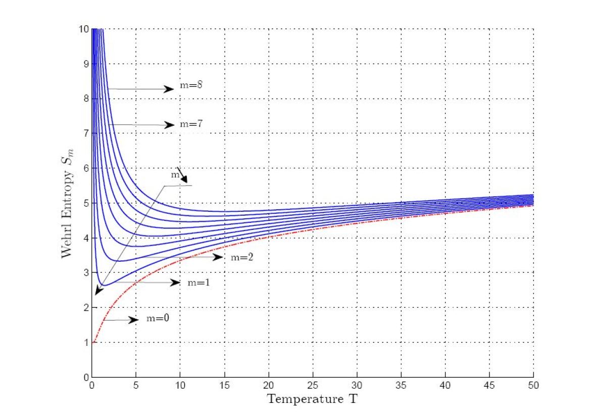
Figure 1. Wehrl entropies $S_{W}\left(\hat{\rho}_{\beta}\right)$ as functions of $T=1/\beta$ for $m=0,1,...8\ .$

Appendix A Proof of equation (3.2)

We compute the scalar product

(A.1) $$\langle\left(x,y\right),B,m\mid\varphi_{j}\rangle=\int_{\mathbb{R}}\langle\xi\mid(x,y),B,m\rangle\overline{\langle\xi\mid\varphi_{j}\rangle}d\xi$$

(A.2) $$=\left(\pi 2^{m+j}m!j!\right)^{-1/2}e^{-\frac{B}{4}(x^{2}+y^{2})}\int_{\mathbb{R}}e^{-\left(\xi+\frac{\sqrt{B}}{2}(iy-x)\right)^{2}}H_{m}(\xi-\sqrt{B}x)\,H_{j}(\xi)\,d\xi$$

By the change of variable $t=\xi+\frac{\sqrt{B}}{2}(iy-x)$, Eq(A.2) becomes

(A.3) $$\langle(x,y),B,m\mid\varphi_{j}\rangle=\frac{e^{-\frac{B}{4}(x^{2}+y^{2})}}{\sqrt{\pi 2^{m+j}m!j!}}\int_{\mathbb{R}}e^{-t^{2}}\,H_{m}\left(t-\frac{\sqrt{B}}{2}(x+iy)\\ \right)\,H_{j}\left(t+\frac{\sqrt{B}}{2}(x-iy)\right)dt.$$

The formula ([14], p.804):

(A.4) $$\int_{-\infty}^{+\infty}e^{-t^{2}}H_{k}(t+u)H_{l}(t+v)\,dt=2^{l}\pi^{\frac{1}{2}}k!v^{l-k}L_{k}^{(l-k)}(-2uv),\,k\leq l,$$

for parameters $u=-\frac{\sqrt{B}}{2}(x+iy)$ and $v=\frac{\sqrt{B}}{2}(x-iy)$ gives

(A.5) $$\langle(x,y),B,m\mid\varphi_{j}\rangle=\sqrt{\frac{m!}{j!}}e^{-\frac{B}{4}(x^{2}+y^{2})}\left(\sqrt{\frac{B}{2}}(x-iy)\right)^{j-m}L_{m}^{(j-m)}\left(\frac{B}{2}(x^{2}+y^{2})\right),\;m\leq j.$$

In the same way, we obtain

(A.6) $$\langle(x,y),B,m\mid\varphi_{j}\rangle=\sqrt{\frac{j!}{m!}}e^{-\frac{B}{4}(x^{2}+y^{2})}\left(-\sqrt{\frac{B}{2}}(x+iy)\right)^{m-j}L_{j}^{(m-j)}\left(\frac{B}{2}(x^{2}+y^{2})\right),\;m\geq j.$$

According to the expression of the Husimi function

(A.7) $$Q^{(m)}_{j}((x,y),B)=\left|\left\langle(x,y),B,m|\varphi_{j}\right\rangle\right|^{2},$$

we get that

(A.8) $$Q^{(m)}_{j}((x,y),B)=\frac{\min(m,j)!}{\max(m,j)!}e^{-\frac{B}{2}(x^{2}+y^{2})}\left(\frac{B}{2}(x^{2}+y^{2})\right)^{|m-j|}\left(L_{\min(m,j)}^{(|m-j|)}\left(\frac{B}{2}(x^{2}+y^{2})\right)\right)^{2}.$$

This ends the proof with $m\wedge j:=\min(m,j)$ and $m\vee j:=\max(m,j)$.$\Box$

Appendix B Proof of proposition 3.1.

The characteristic function of the probability distribution $Q^{(m)}_{j}((x,y),B)$ is expressed as

(B.1) $$\Phi_{Q^{(m)}_{j}}(u)=\frac{(m\wedge j)!}{(m\vee j)!}\int_{\mathbb{R}^{2}}\mathrm{e}^{(iu-1)\frac{B}{2}(x^{2}+y^{2})}\Big{(}\frac{B}{2}(x^{2}+y^{2})\Big{)}^{|m-j|}\Big{(}L_{m\wedge j}^{(|m-j|)}\Big{(}\frac{B}{2}(x^{2}+y^{2})\Big{)}^{2}\,d\mu(x,y)$$

where $d\mu(x,y)=(2\pi)^{-1}Bdxdy$. Using the polar coordinates $x=r\cos\theta,y=r\sin\theta,\ r>0,\theta\in[0,2\pi)$ and setting $\lambda=Br^{2}/2=B\left(x^{2}+y^{2}\right)/2$ we arrive at

(B.2) $$\Phi_{Q^{(m)}_{{}_{j}}}(u)=\frac{(m\wedge j)!}{(m\vee j)!}\int_{0}^{+\infty}\mathrm{e}^{(iu-1)\lambda}\lambda^{|m-j|}\Big{(}L_{m\wedge j}^{(|m-j|)}(\lambda)\Big{)}^{2}\,d\lambda.$$

Using the formula ([14],p.809):

$$\int_{0}^{+\infty}x^{\alpha}\mathrm{e}^{-bx}L_{m}^{(\alpha)}(\gamma x)L_{n}^{(\alpha)}(\mu x)\,dx=\frac{\Gamma(n+m+\alpha+1)}{m!n!}\frac{(b-\gamma)^{m}(b-\mu)^{n}}{b^{n+m+\alpha+1}},$$

(B.3) $$\times{}_{2}\!F_{1}\left(-m,-n;-m-n-\alpha;\,b(b-\gamma-\mu)((b-\gamma)(b-\mu))^{-1}\right),$$

where $\Re(\alpha)>-1$ and $\Re(b)>-1$, we obtain with $b=1-it,n=m\wedge j,\alpha=|m-j|$ and $\gamma=\mu=1$

(B.4) $$\Phi_{Q^{(m)}_{j}}(u)=\frac{(m+j)!}{m!j!}\frac{(-1)^{m\wedge j}u^{2(m\wedge j)}}{(1-it)^{m+j+1}}\ {}_{2}F_{1}\left(-(m\wedge j),-(m\wedge j);-m-j;(1+u^{2})u^{-2}\right).$$

By the Pffaf’s transformation ([36],p.47):

(B.5) $${}_{2}\!F_{1}(a,b;c;z)=(1-z)^{-a}\,{}_{2}\!F_{1}\left(a,c-b;c;z(1-z)^{-1}\right),\quad z\in\mathbb{C},$$

we obtain finally

(B.6) $$\Phi_{Q^{(m)}_{{}_{j}}}(u)=\frac{(m+j)!}{m!j!}(1-iu)^{-(m+j+1)}\,{}_{2}\!F_{1}\left(-(m\wedge j),-(m\vee j);-m-j;\,1+u^{2}\right).$$

The moments of the variable $Q^{(m)}_{j}$ are obtained from the characteristic function repeating differentiation with respect to the variable $u$ and evaluated at the origin as

(B.7) $$\mathbb{E}((Q^{(m)}_{j})^{k})=\left.\frac{1}{i^{k}}\frac{\partial^{k}}{\partial u^{k}}\Phi_{Q^{(m)}_{j}}(u)\right|_{u=0}.$$

The differentiation of the hypergeometric function ${}_{2}\!F_{1}(\cdot)$ ([36],p.41) gives the mean value

(B.8) $$\mathbb{E}(Q^{m}_{j})=\frac{(m+j)!}{m!j!}(m+j+1)\,{}_{2}\!F_{1}\left(-(m\wedge j),-(m\vee j),-m-j;\,1+u^{2}\right)|_{u=0}.$$

We have from ([36],p.212):

(B.9) $${}_{2}\!F_{1}\left(-(m\wedge j),-(m\vee j),-m-j;\,1\right)=\frac{m!j!}{(m+j)!}.$$

Then $\mathbb{E}(Q^{(m)}_{j})=m+j+1$. For the variance, we need the second order moment of $Q^{(m)}_{\hat{\rho}_{j}}$ by applying (B.7) for $k=2$. We find

$$\mathbb{E}\left((Q^{m}_{j})^{2}\right)=\frac{(m+j)!}{m!j!}(m+j+1)(m+j+2){}_{2}\!F_{1}\left(-(m\wedge j),-(m\vee j),-m-j;\,1+u^{2}\right)|_{u=0}$$

(B.10) $$+\frac{(m+j)!}{m!j!}\frac{2mj}{m+j}\,{}_{2}\!F_{1}\left(-(m\wedge j-1),-(m\vee j-1),-(m+j-1);\,1+u^{2}\right)|_{u=0}$$

which reduces to $(m+j+1)(m+j+2)+2mj.$ The well-known formula of the variance gives $\mathcal{V}ar(Q^{(m)}_{j})=2mj+m+j+1.$ This ends the proof. $\Box$

Appendix C Proof of proposition 3.2.

From (3.13), the Husimi function of the mixed state $\hat{\rho}_{\beta}$ is expressed by

(C.1) $$Q^{(m)}_{\beta}((x,y),B)=\frac{1}{Z}\sum_{j=0}^{+\infty}e^{-\beta\left(j+\frac{1}{2}\right)}Q^{(m)}_{j}((x,y),B)$$

According to remark 3.2, Eq.$(\ref{hhusimi})$ reads

(C.2) $$Q^{(m)}_{\beta}(\lambda,B)=\frac{e^{-\left(\lambda+\frac{\beta}{2}\right)}}{Z}\sum_{j=0}^{+\infty}e^{-\beta j}\frac{(m\land j)!}{(m\lor j)!}\lambda^{|m-j|}\left(L_{m\land j}^{(|m-j|)}(\lambda)\right)^{2}.$$

We start by computing the following series

(C.3) $$\mathcal{O}_{\beta,\lambda,m}:=\sum_{j=0}^{+\infty}e^{-\beta j}\frac{(m\land j)!}{(m\lor j)!}\lambda^{|m-j|}\left(L_{m\land j}^{(|m-j|)}(\lambda)\right)^{2}$$

$$=\sum_{j=0}^{m-1}e^{-\beta j}\frac{j!}{m!}\lambda^{m-j}\left(L_{j}^{(m-j)}(\lambda)\right)^{2}-\sum_{j=0}^{m-1}e^{-\beta j}\frac{m!}{j!}\lambda^{j-m}\left(L_{m}^{(j-m)}(\lambda)\right)^{2}+\sum_{j=0}^{+\infty}e^{-\beta j}\frac{m!}{j!}\lambda^{j-m}\left(L_{m}^{(j-m)}(\lambda)\right)^{2}.$$

We denote by $S_{f}$ the finite sum

(C.4) $$S_{f}=\sum_{j=0}^{m-1}e^{-\beta j}\left[\frac{j!}{m!}\lambda^{m-j}\left(L_{j}^{(m-j)}(\lambda)\right)^{2}-\frac{m!}{j!}\lambda^{j-m}.\left(L_{m}^{(j-m)}(\lambda)\right)^{2}\right].$$

Applying the formula ([37] p.552):

(C.5) $$L_{m}^{(-k)}(x)=(-x)^{k}\frac{(m-k)!}{m!}L_{m-k}^{(k)}(x),\quad 1\leq k\leq m,$$

in the case $0\leq(k=m-j)\leq m$ since $j=0,1,\cdots m-1$, we find

(C.6) $$L_{m}^{(j-m)}(\lambda)=(-1)^{m-j}\lambda^{(m-j)}\frac{j!}{m!}L_{j}^{(m-j)}(\lambda).$$

Then $(\ref{C5})$ becomes

(C.7) $$S_{f}=\sum_{j=0}^{m-1}e^{-\beta j}\left[\frac{j!}{m!}\lambda^{m-j}\left(L_{j}^{(m-j)}(\lambda)\right)^{2}-\frac{j!}{m!}\lambda^{(m-j)}\left(L_{j}^{m-j}(\lambda)\right)^{2}\right]=0.$$

So that $\mathcal{O}_{\beta,\lambda,m}$ takes the form

(C.8) $$\mathcal{O}_{\beta,\lambda,m}=\frac{m!}{\lambda^{m}}\sum_{j=0}^{+\infty}\frac{(e^{-\beta}\lambda)^{j}}{j!}\left(L_{m}^{(j-m)}(\lambda)\right)^{2}.$$

With the help of Wicksell-Campbell-Meixner formula ([38], p. 279):

(C.9) $$\sum_{n=0}^{+\infty}\frac{u^{n}}{n!}L_{l}^{(n-l)}(\xi)L_{k}^{(n-k)}(\zeta)=e^{u}\frac{u^{l}(u-\zeta)^{k-l}}{k!}L_{l}^{(k-l)}\left(-\frac{(\xi-u)(\zeta-u)}{z}\right)$$

for parameters $l=k=m,n=j,\xi=\zeta=\lambda$ and $u=e^{-\beta}\lambda$, we obtain the expression

(C.10) $$\mathcal{O}_{\beta,\lambda,m}=\exp\left(\lambda e^{-\beta}-\beta m\right)L^{(0)}_{m}\left(-\lambda\left(1-e^{-\beta}\right)^{2}e^{\beta}\right).$$

from which, (C.2) becomes

(C.11) $$Q^{(m)}_{\beta}(\lambda,B)=\frac{1}{Z}\exp\left(\lambda(e^{-\beta}-1)-\beta\left(m+\frac{1}{2}\right)\right)L^{(0)}_{m}\left(-\lambda\left(1-e^{-\beta}\right)^{2}e^{\beta}\right).$$

For the harmonic oscillator $Z=Tr\left(e^{-\beta\hat{H}}\right)=1/\left(e^{\beta/2}-e^{-\beta/2}\right)$. This gives

(C.12) $$Q^{(m)}_{\beta}(\lambda,B)=(e^{\beta/2}-e^{-\beta/2})\exp\left(\lambda(e^{-\beta}-1)-\beta\left(m+\frac{1}{2}\right)\right)L^{(0)}_{m}\left(-\lambda\left(1-e^{-\beta}\right)^{2}e^{\beta}\right).$$

Finally, by replacing $\lambda$ by the expression $B(x^{2}+y^{2})/2$, we obtain the result.                     $\Box$

Appendix D Proof of proposition 4.1.

The Wehrl entropy for the Husimi function (3.2) is defined by

(D.1) $$\mathcal{S}_{W}(\hat{\rho}_{j}):=-\int_{\mathbb{R}^{2}}Q^{(m)}_{j}((x,y),B)\log Q^{(m)}_{j}((x,y),B)d\mu(x,y).$$

Using the polar coordinates $x=r\cos\theta,\ y=r\sin\theta$ with $r>0$, $\theta\in[0,2\pi)$ and setting $t=\frac{B}{2}r^{2}$, we rewrite $(\ref{WehrlJJ1})$ as

$$\mathcal{S}_{W}(\hat{\rho}_{j}) = -\frac{(m\land j)!}{(m\lor j)!}\int_{0}^{+\infty}\left[\mathrm{e}^{-t}t^{|m-j|}\left(L_{m\land j}^{(|m-j|)}(t)\right)^{2}\right]\log\left[\frac{(m\land j)!}{(m\lor j)!}\mathrm{e}^{-t}t^{|m-j|}\left(L_{m\land j}^{(|m-j|)}(t)\right)^{2}\right]dt$$

We split this integral into four integrals as follows

$$\mathcal{S}_{W}(\hat{\rho}_{j}) = -\frac{(m\land j)!}{(m\lor j)!}\int_{0}^{+\infty}\left[\mathrm{e}^{-t}t^{|m-j|}\left(L_{m\land j}^{(|m-j|)}(t)\right)^{2}\right]dt$$

$$+\frac{(m\land j)!}{(m\lor j)!}\int_{0}^{+\infty}\left[\mathrm{e}^{-t}t^{|m-j|+1}\left(L_{m\land j}^{(|m-j|)}(t)\right)^{2}\right]\,dt$$

$$-\frac{(m\land j)!}{(m\lor j)!}|m-j|\int_{0}^{+\infty}\left[\mathrm{e}^{-t}t^{|m-j|}\left(L_{m\land j}^{(|m-j|)}(t)\right)^{2}\right]\log t\,dt$$

$$-\frac{(m\land j)!}{(m\lor j)!}\int_{0}^{+\infty}\left[\mathrm{e}^{-t}t^{|m-j|}\left(L_{m\land j}^{(|m-j|)}(t)\right)^{2}\right]\log\left[\frac{(m\land j)!}{(m\lor j)!}\left(L_{m\land j}^{(|m-j|)}(t)\right)^{2}\right]dt.$$

The orthogonally relation of Laguerre polynomials gives

(D.2) $$I_{1} := -\frac{(m\land j)!}{(m\lor j)!}\int_{0}^{+\infty}\left[\mathrm{e}^{-t}t^{|m-j|}\left(L_{m\land j}^{(|m-j|)}(t)\right)^{2}\right]dt=-1$$

From Srivastava’s formula ([39],p.1133):

(D.3) $$\int_{0}^{+\infty}t^{\alpha+s}\mathrm{e}^{-t}\left(L_{n}^{(\alpha)}(t)\right)^{2}\,dt=\sum_{r=0}^{n}\binom{s}{n-r}^{2}\frac{\Gamma(\alpha+s+r+1)}{r!},\;\Re\alpha>-1.$$

for $n=m\land j,\alpha=|m-j|$ and $s=1$, the seconde integral reads

(D.4) $$I_{2} := \frac{(m\land j)!}{(m\lor j)!}\int_{0}^{+\infty}\left[\mathrm{e}^{-t}t^{|m-j|+1}\left(L_{m\land j}^{(|m-j|)}(t)\right)^{2}\right]dt=m+j+1.$$

Next, the use of formula ([40],p.27):

$$\int_{0}^{+\infty}\mathrm{e}^{-t}t^{\alpha+s}\left(L_{n}^{(\alpha)}(t)\right)^{2}\log t\,dt = \sum_{r=0}^{n}\binom{s}{n-r}^{2}\frac{\Gamma(\alpha+s+r+1)}{r!}$$

$$\times \Big{[}2\psi(s+1)+\psi(\alpha+s+r+1)-2\psi(s+r+1-n)\Big{]}$$

with $\Re\alpha>-1$ and $\psi(z)$ the digamma function, allows to write the third integral as follows

(D.5) $$I_{3}: = -\frac{(m\land j)!}{(m\lor j)!}|m-j|\int_{0}^{+\infty}\left[\mathrm{e}^{-t}t^{|m-j|}\left(L_{m\land j}^{(|m-j|)}(t)\right)^{2}\right]\log t\,dt$$

(D.6) $$= -|m-j|(m\lor j+1)\psi(m\lor j+1).$$

Making use of the formula ([41],p.3052):

$$\frac{n!}{\Gamma(n+\alpha+1)}\int_{0}^{+\infty}\mathrm{e}^{-t}t^{s}\left(L_{n}^{(\alpha)}(t)\right)^{2}\log\left[\frac{n!}{\Gamma(n+\alpha+1)}\left(L_{n}^{(\alpha)}(t)\right)^{2}\right]\,dt=\frac{2^{2s+2}\Gamma(s+3/2)}{\sqrt{\pi}\Gamma(s+2)}n^{s+1}$$

$$-\frac{2^{2s}(\alpha+1)\Gamma(s+1/2)}{\sqrt{\pi}\Gamma(s+1)}n^{s}\log n+\frac{2^{2s-1}\Gamma(s+1/2)}{\sqrt{\pi}\Gamma(s+1)}\Big{[}2(\alpha+1)\psi(s+1)-(2\alpha+1)\psi(s+1/2)-2\log\pi$$

(D.7) $$-4(\alpha+1)\log 2+\gamma_{E}+4+2(\alpha+2s)+4\alpha s\Big{]}n^{s}+o(n^{s})$$

with $\Re\alpha>-1$ and $\gamma_{E}$ the Euler constant, the last integral expresses as

(D.8) $$I_{4} := -\frac{(m\land j)!}{(m\lor j)!}\int_{0}^{+\infty}\left[\mathrm{e}^{-t}t^{|m-j|}\left(L_{m\land j}^{(|m-j|)}(t)\right)^{2}\right]\log\left[\frac{(m\land j)!}{(m\lor j)!}\left(L_{m\land j}^{(|m-j|)}(t)\right)^{2}\right]\,dt$$

$$= -m-j+(|m-j|+1)\log(m\land j)+\log 2\pi-2+o(1).$$

Finally, replacing the four integrals by their respective expressions, it follows that

$$\mathcal{S}_{W}(\hat{\rho}_{j}) = -|m-j|(m\lor j+1)\psi(m\lor j+1)+(|m-j|+1)\log(m\land j)+\log 2\pi-1+o(1).$$

From the asymptotic behavior of the digamma function ([31]):

(D.9) $$\psi(m\lor j+1)=\log(m\lor j+1)+o(1)$$

we obtain the announced result $(\ref{entrropy})$ and the inequality is immediate. This ends the proof.$\Box$

References

- [1] S. T. Ali, J. P. Antoine and J. P. Gazeau, Coherent States, Wavelets and Their Generalizations, second edition, Springer Science+Business Media New York (2014)
- [2] K. Husimi, Some Formal Properties of the Density Matrix, Proc. Phys. Math. Soc. Jpn. 22, 264-314, 1940
- [3] Rov J. Glauber, The quantum Theory of optical coherence, Phys. Rev. 130, 2529, 1963
- [4] A. Wehrl, General properties of entropy, Rev. Mod. Phys., 50, 221, 1978
- [5] A. Orlowski, Wehrl Entropy and Classification of States, Rep. Math. Phys., 43, 283-289, 1999
- [6] E. H. Lieb, Proof of an entropy Conjecture of Wehrl, Commun. math. Phys. 62, 35-41, 1978
- [7] Z. Mouayn, A Generating Function for Hermite Polynomials Associated with Euclidean Landau Levels, Theoritical and Mathematical Physics, 165, 1435-1442, 2010
- [8] L. D. Abreu, Sampling and interpolation in Bargmann-Fock spaces of polyanalytic functions, Appl. Comp. Harm. Anal., 29 (2010), 287-302.
- [9] Z. Mouayn, Coherent State transforms attached to generalized Bargmann space on the complex plane, Math. Nachr, 284, 1-7, 2011
- [10] Z. Mouayn, Characterization of two-dimensional Euclidean Landau states by coherent state transforms, J. Phys A: Math. Gen., 37, 8071, 2004
- [11] A. Perelomov, Generalized coherent states an their Application, New York: Springer (1986)
- [12] P. Kral. Displaced and squeezed Fock states. Journal of Modern Optics, 37(5):889-917, (1990)
- [13] V. V. Dodonov. ’Nonclassical’ states in quantum optics: a ’squeezed’ review of the first 75 years. J. Opt. B: Quantum Semiclass. Opt. 4:R1?R33, (2002)
- [14] I. S. Gradshteyn and I.M. Ryzhik. Table of integrals, series and products, Seventh edition. Academic Press (2007)
- [15] L. D. Abreu, P. Balazs, M. A de Gosson and Z. Mouayn, Discrete coherent states for higher Landau levels, Ann. Phys, 363, 337-353, 2015.
- [16] L. D. Abreu, On the structure of Gabor and super Gabor spaces, Monatsh. Math., 161 (2010), 237-253.
- [17] K. Gröchenig, A. Haimi, J. L Romero, Completeness of Gabor systems, J. Aprox. Theor. 207 (2016), 283-300.
- [18] J. P. Gazeau, Coherent states in Quantum Physics, WILEY-VCH Verlag GmbH & Co. KGaA, Weinheim (2009)
- [19] H. J. Korsh, C. Müller and H. Wiescher, On the zeros of the Husimi distribution, J. Phys A: Math. Gen., 30, L677-L684, 1997
- [20] P. S. Moreno, D. Manzeno and J. S. Dehesa, Direct spreading measures of Laguerre polynomials, J. Comput. Appl. Math., 235, 1129-1140, 2011
- [21] T. Shirai, Ginibre-type point processes and their asymptotic behavior, J. Math. Soc. Japan, 67 763-787, 2015
- [22] L. D. Abreu, J. Pereira, J. L. Romero, S. Torquato, The Weyl-Heisenberg ensembles: hyperuniformity and higher Landau Levels, Journal of Statistical Mechanics: Theory and Experiment, 2017(4), 043103.
- [23] A. Haimi, H. Hedenmalm, The polyanalytic Ginibre ensembles, J. Stat. Phys. 153:1, (2013), 10-47.
- [24] A. Haimi, H. Hedenmalm, Asymptotic expansions of polyanalytic Bergman kernels. J. Funct. Anal., 267, 4667-4731 (2014).
- [25] Z. Mouayn and A. Touhami, Probability distributions attached to generalized Bargmann-Fock spaces in the complex plane, Infin. Dimens. Anal. Quantum. Probab. Relat., 13, 257-271, 2010
- [26] N. Demmi and Z. Mouayn, Analysis of photon-counting probability distribution attached to euclidean Landau levels, Infin. Dimens. Anal. Quantum. Probab. Relat., 18, 1550028, 2015
- [27] A. P. Prudnikov, Yu. A. Brychkov and O. I. Marichev, Integrals and Series, More Special Functions, vol 3, Gordon and Breach science publisher (1990)
- [28] A. Dembo and O. Zeitouni, Large Deviation Techniques and Applications, 2nd edition, Springer-Verlag New York, Inc. (1998)
- [29] J. Perina, Superposition of thermal and coherent fields, Acta Universitatis Palackianae Olomucencis. Facultas Rerum Naturalium. Mathematica, Vol. 9, 227-234, 1968
- [30] A. A. Semenov, A. V. Turchin and H. V. Gomonay, Detection of quantum light in the presence of noise, Phys. Rev. A., 78, 055803, 2008, 79, 019902(E), 2009
- [31] M. Martinelli and P. Martelli, Laguerre Mathematics in optical communication, Opt. Photonics News 19, 30-35, 2008
- [32] L. Comptet, Advanced Combinatorics, D. Reidel Publishing Company, Dordrecht (1974)
- [33] H. M. Srivastava and A.W. Niukkanen, Some Clebsh-Gordan type liberalization relation and associated families of Dirichlet Integrals, Math Comput Model, 37, 245-250, 2003
- [34] A. M. Mathai and Hans J. Houbold, Special functions for applied scientists, Springer Science+Business Media, LLC (2008)
- [35] A. Anderson and J. J. Halliwell, Information-theoretic measure of uncertainty due to quantum and thermal fluctuations, Phys. Rev., 48, 2753, 1993
- [36] W. Magnus, F. Oberhettinger and R.P. Soni. Formulas and Theorems for the Special Functions of Mathematical and Physics. Springer-Verlag, Berlin, Heidelberg (1941)
- [37] Y. A. Brychkov, Handbook of Special Function derivative, integrals and others formulas, CRC Press (2008)
- [38] H. M. Srivastava and H.L. Manocha, A treatise on Generating Functions, Ellis Horwood limites (1984)
- [39] R. S. Alassar H. A. Mavromatis and H.M. Srivastava. Remarks on some associated Laguerre integral results, Appl. Math. Lett., 16, 1131-1136, 2003
- [40] J. S. Dehesaa, A. Martinez-Finkelshteinc and J. Sanchez-Ruiz. Quantum information entropies and orthogonal polynomials, J. Comput. Appl. Math., 133, 23-46, 2001
- [41] J. S. Dehesa, R.J. Yanez, A. I. Aptekarev and V. Buyarov. Strong asymptotics of Laguerre polynomials and information entropies of two-dimensional harmonic oscillator and one-dimensional Coulomb potentials, J. Comput. Appl. Math., 39, 3050-3060, 1998
-
[42]
M. Abramovitz and I. A. Stegun. Handbook of
Mathematical Functions with formulas, graphs, and mathematical tables,
National Bureau of Standards, Applied Mathematics Series (1964)
∗ Department of Mathematics, Faculty of Sciences and Technics (M’Ghila), P.O.Box. 523, Béni Mellal, Morocco.
mouayn@gmail.com
⋄ Departement of Mathematics, Faculty of sciences and technics, University Abdelmalek Essaâdi, P.O.Box. 416, Tangier, Morocco.
hamidoukass@gmail.com
♯ Department of Mathematics, Faculty of Sciences, Ibn Tofail University, P.O.Box. 133, Kénitra, Morocco.
kayupepatrick@gmail.com
♭ Department of Network and Telecommunications Engineering, LISERT, National School of Applied Sciences (ENSA), Hassan 1 University, P.O. Box 77, Khouribga, Morocco.
fatani.imade@gmail.com