Sharp Degree Bounds for Sum-of-Squares Certificates
on Projective Curves

Abstract.

Given a real projective curve with homogeneous coordinate ring $R$ and a nonnegative homogeneous element $f\in R$, we bound the degree of a nonzero homogeneous sum-of-squares $g\in R$ such that the product $fg$ is again a sum of squares. Better yet, our degree bounds only depend on geometric invariants of the curve and we show that there exist smooth curves and nonnegative elements for which our bounds are sharp. We deduce the existence of a multiplier $g$ from a new Bertini Theorem in convex algebraic geometry and prove sharpness by deforming rational Harnack curves on toric surfaces. Our techniques also yield similar bounds for multipliers on surfaces of minimal degree, generalizing Hilbert’s work on ternary forms.

1. Overview of Results

Certifying that a polynomial is nonnegative remains a central problem in real algebraic geometry and optimization. The quintessential certificate arises from multiplying a given polynomial by a second polynomial, that is already known to be positive, and expressing the product as a sum of squares. Although the Positivstellensatz guarantees that suitable multipliers exist over any semi-algebraic set, tight bounds on the degree of multipliers are exceptionally rare. Our primary aim is to produce sharp degree bounds for sum-of-squares multipliers on real projective curves. In reaching this goal, the degree bounds also reveal a surprising consonance between real and complex algebraic geometry.

To be more explicit, fix an embedded real projective curve $X\subset\mathbb{P}^{n}$ that is nondegenerate and totally real—not contained in a hyperplane and with Zariski-dense real points. Let $R$ be its $\mathbb{Z}$-graded coordinate ring and let $\operatorname{r}(X)$ denote the least integer $i$ such that the Hilbert polynomial and function of $X$ agree at all integers greater than or equal to $i$. For $j\in\mathbb{N}$, we write $\operatorname{P}_{X,2j}\subset R_{2j}$ and $\operatorname{\Sigma}_{X,2j}\subset R_{2j}$ for the cone of nonnegative elements in $R_{2j}$ and the cone of sums of squares of elements from $R_{j}$, respectively. Our first result gives a sharp degree bound on sum-of-squares multipliers in terms of the fundamental geometric invariants of $X$.

Theorem 1.1.

For any nondegenerate totally-real projective curve $X\subset\mathbb{P}^{n}$ of degree $d$ and arithmetic genus $p_{\text{a}}$, any nonnegative element $f\in\operatorname{P}_{X,2j}$ of positive degree, and all $k\in\mathbb{N}$ satisfying $k\geqslant\max\bigl{\{}\operatorname{r}(X),\frac{2p_{\text{a}}}{d}\bigr{\}}$, there is a nonzero $g\in\operatorname{\Sigma}_{X,2k}$ such that $fg\in\operatorname{\Sigma}_{X,2j+2k}$. Conversely, for all $n\geqslant 2$ and all $j\geqslant 2$, there exist totally-real smooth curves $X\subset\mathbb{P}^{n}$ and nonnegative elements $f\in\operatorname{P}_{X,2j}$ such that, for all $k<\max\bigl{\{}\operatorname{r}(X),\frac{2p_{\text{a}}}{d}\bigr{\}}$ and for all nonzero $g\in\operatorname{\Sigma}_{X,2k}$, we have $fg\not\in\operatorname{\Sigma}_{X,2j+2k}$.

Remarkably, the uniform degree bound on the multiplier $g$ is determined by the complex geometry of the curve $X$. It is independent of both the degree of the nonnegative element $f$ and the Euclidean topology of the real points in $X$.

Our approach also applies to higher-dimensional varieties that are arithmetically Cohen–Macaulay, but it is most effective on certain surfaces. A subvariety $X\subset\mathbb{P}^{n}$ has minimal degree if it is nondegenerate and $\deg(X)=1+\operatorname{codim}(X)$. Theorem 1.1 in [BSV] establishes that $\operatorname{P}_{X,2}=\operatorname{\Sigma}_{X,2}$ if and only if $X$ is a totally-real variety of minimal degree. Evocatively, this equivalence leads to a characterization of the varieties over which multipliers of degree zero suffice. Building on this framework and generalizing Hilbert’s work [Hilbert2] on ternary forms, our second result gives degree bounds for sum-of-squares multipliers on surfaces of minimal degree.

Theorem 1.2.

If $X\subset\mathbb{P}^{n}$ is a totally-real surface of minimal degree and $f\in\operatorname{P}_{X,2j}$ is a nonnegative element of positive degree, then there is a nonzero $g\in\operatorname{\Sigma}_{j^{2}-j}$ such that $fg\in\operatorname{\Sigma}_{X,j^{2}+j}$. Conversely, if $X\subset\mathbb{P}^{n}$ is a totally-real surface of minimal degree and $j\geqslant 2$, then there exist nonnegative elements $f\in\operatorname{P}_{X,2j}$ such that, for all $k<j-2$ and all nonzero $g\in\operatorname{\Sigma}_{X,2k}$, we have $fg\not\in\operatorname{\Sigma}_{X,2j+2k}$.

Unlike curves, Theorem 1.2 shows that the minimum degree of a sum-of-squares multipler $g$ depends intrinsically on the degree of the nonnegative element $f$. The sharpness of the upper or lower bounds on these surfaces is an intriguing open problem.

Motivated by its relation to Hilbert’s Seventeenth Problem, we obtain slightly better degree bounds when the totally-real surface is $\mathbb{P}^{2}$; see Example 4.18 and Example 5.17 for the details. Specifically, we re-prove and prove the following two results for ternary octics:

• for all nonnegative $f\in\operatorname{P}_{\mathbb{P}^{2},8}$, there exists a nonzero $g\in\operatorname{\Sigma}_{\mathbb{P}^{2},4}$ such that $fg\in\operatorname{\Sigma}_{\mathbb{P}^{2},12}$; and

• there exists a nonnegative $f\in\operatorname{P}_{\mathbb{P}^{2},8}$ such that, for all nonzero $g\in\operatorname{\Sigma}_{\mathbb{P}^{2},2}$, we have $fg\not\in\operatorname{\Sigma}_{\mathbb{P}^{2},10}$.

Together these give the first tight bounds on the degrees of sum-of-squares multipliers for homogeneous polynomials since Hilbert’s 1893 paper [Hilbert2] in which he proves sharp bounds for ternary sextics. No other sharp bounds for homogeneous polynomials are known. For example, the recent theorem in [Pas] shows that, for quaternary quartics, one can multiply by sum-of-squares of degree $4$ to obtain a sum of squares, but it is not known whether quadratic multipliers suffice.

By reinterpreting Theorem 1.1 or Theorem 1.2, we do obtain degree bounds for certificates of nonnegativity. A sum-of-squares multiplier $g$ certifies that the element $f$ is nonnegative at all points where $g$ does not vanish. When the complement of this vanishing set is dense in the Euclidean topology, it follows that the element $f$ is nonnegative. Changing perspectives, these theorems also generate a finite hierarchy of approximations to the cone $\operatorname{P}_{X,2j}$, namely the sets $\{f\in R_{2j}:\text{there exists $g\in\operatorname{\Sigma}_{X,2k}$ such that $fg\in\operatorname{\Sigma}_{X,2j+2k}$}\}$; compare with Subsection 3.6.1 in [BPT]. It follows that deciding if an element $f$ belongs to the cone $\operatorname{P}_{X,2j}$ is determined by a semidefinite program of known size.

Relationship with prior results

Our degree bounds, with their uniformity and sharpness, cannot be directly compared to any established bound on multipliers, except for those on zero-dimensional schemes in [BGP]. Most earlier work focuses on general semi-algebraic sets, where no sharpness results are known, or on affine curves, where no uniform bounds are possible for singular curves.

The best bound on the degree of a sum-of-squares multiplier on an arbitrary semi-algebraic set involves a tower of five exponentials; see Theorem 1.5.7 in [LPR]. However, Corollary 4.9 shows that, for a nondegenerate totally-real projective curve $X\subset\mathbb{P}^{n}$ of degree $d$, every nonnegative form admits a nonzero sum-of-squares multiplier of degree $2k$ for all $k\geqslant d-n+1$. Absent sharp bounds in some larger context, it impossible to ascertain if this difference in the complexity of the bounds is just a feature of low-dimensional varieties or part of some more general phenomenon.

Restricting to curves likewise fails to produce meaningful comparisons. Corollary 4.15 in [ScheidererC] illustrates that one can often certify nonnegativity without using a multiplier on an affine curve. Concentrating on a special type of multiplier, Theorem 4.11 in [ScheidererP] demonstrates that, on a nonsingular projective curve, any sufficiently large power of a positive element gives a multiplier; also see [Rez]. For nonsingular affine curves, Corollary 4.4 in [ScheidererS] establishes that there exist uniform degree bounds, even though the techniques do not yield explicit results. In contrast with Theorem 1.1, the bounds in these situations either depend on the nonnegative element $f$ or tend towards positive infinite as the underlying curve acquires certain singularities.

To identify a close analogue of our work, we must lower the dimension: Theorems 1.1–1.2 in [BGP] provide uniform degree bounds over a finite set of points that are tight for quadratic functions on the hypercube. The lone additional sharp degree bound on multipliers is, to the best of our knowledge, Hilbert’s original work [Hilbert2] on ternary sextics.

Main ideas

The results in this paper arose while exploring the relationship between convex geometry and algebraic geometry for sums of squares on real varieties. The two parts of our main theorems are proven independently. The upper bound on the minimum degree of a sum-of-squares multiplier is derived from a new Bertini Theorem in convex algebraic geometry and the lower bound is obtained by deforming rational Harnack curves on toric surfaces.

To prove the first part, we reinterpret the non-existence of a sum-of-squares multiplier $g\in\operatorname{\Sigma}_{X,2k}$ as asserting that the convex cones $\operatorname{\Sigma}_{X,2j+2k}$ and $f\cdot\operatorname{\Sigma}_{X,2k}$ intersect only at zero. If a real subscheme $X\subseteq\mathbb{P}^{n}$ possesses a linear functional separating these cones, then Theorem 3.1 demonstrates that a sufficiently general hypersurface section of $X$ also does. In this setting, the phrase ‘sufficiently general’ means belonging to a nonempty open subset in the Euclidean topology of the relevant parameter space. Unexpectedly, this convex version of Bertini’s Theorem relies on our characterization of spectrahedral cones that have many facets in a neighbourhood of every point; see Proposition 2.5. Recognizing this dependency is the crucial insight. By repeated applications of our Bertini Theorem, we reduce to the case of points. Theorem 4.3 establishes the degree bound for the existence of a sum-of-squares multiplier on curves and Theorem 4.13 gives a higher-dimensional variant on arithmetically Cohen–Macaulay varieties.

To prove the second part, we show that having a nonnegative element vanish at a relatively large number of isolated real singularities precludes it from having a low-degree sum-of-squares multiplier. As Proposition 5.5 indicates, the hypotheses needed to actually realize this basic premise are formidable. Nonetheless, this transforms the problem into finding enough curves that satisfy the conditions and maximize the number of isolated real singularities. Proposition 5.7 confirms that rational singular Harnack curves on toric surfaces fulfill these requirements. By perturbing both the curve $X$ and the nonnegative element $f\in R_{2j}$, Theorem 5.8 exhibits smooth curves and nonnegative elements without low-degree sum-of-squares multipliers. Proposition 5.15 then lifts these degree bounds from curves to some surfaces. Miraculously, for totally-real projective curves, the degree bounds in Theorem 4.3 and Theorem 5.8 coincide.

Explicit Examples

Beyond the uniformity, our results also specialize to simple degree bounds in many interesting situations. As one might expect, the degree bounds are straightforward for complete intersections and planar curves; see Example 4.6 and Example 4.7. However, by demonstrating that our degree bound is sharp for some, but not all, planar curves, Example 4.8 and Example 5.3 are much more innovative. For certain non-planar curves lying on embedded toric surfaces, Examples 5.11–5.14 present sharp degree bounds. These examples also serve as our best justification for the second part of Theorem 1.1. It remains an open problem to classify all of the curves for which the bounds in Theorem 1.1 are sharp. Switching to higher-dimensional arithmetically Cohen–Macaulay varieties, Example 4.16 re-establishes that a nonnegative quadratic form on a totally-real variety of minimal degree is a sum of squares. Examples 4.17–4.19, which bound multipliers on surfaces of minimal degree, the projective plane, and surfaces of almost minimal degree respectively, appear to exhaust all of the consequential applications to surfaces. Together Example 4.17 and Example 5.16 establish Theorem 1.2. Highlighting the peculiarity of curves, this pair of examples also illustrates the gap between our upper and lower bounds on the minimal degree of a multiplier in this case. Nevertheless, Example 5.17 does give our new sharp bound for ternary octics. Despite being labelled examples, these are essential aspects of the paper.

2. Many-Faceted Spectrahedral Cones

This section focuses on convex geometry and properties of spectrahedral cones. We distinguish certain spectrahedral cones that have an abundance of facets in the vicinity of every point. To demonstrate the ubiquity of these cones in convex algebraic geometry, we show that if a sum-of-squares cone is closed and contains no lines, then its dual has this structure.

Let $V$ be a finite-dimensional real vector space, let $S_{2}\mathrel{\mathop{:}}=\operatorname{Sym}^{2}(V^{*})$ be the vector space of quadratic forms on $V$, and let $S_{2}^{+}\subseteq S_{2}$ be the cone of positive-semidefinite quadratic forms. The corank of a quadratic form $f\in S_{2}$ is the dimension of the kernel $\operatorname{Ker}(f)$ of the associated symmetric matrix. We endow $\operatorname{Sym}^{2}(V^{*})$ with the metric topology arising from the spectral norm. Since all norms on a finite-dimensional vector space induce the same topology, we refer to this metric topology as the Euclidean topology. For a quadratic form $g\in S_{2}$ and a positive real number $\varepsilon$, we write $B_{\varepsilon}(g)\subset S_{2}$ for the open ball of radius $\varepsilon$ centered at $g$. As usual, we equip each subset $W\subseteq S_{2}$ with the induced Euclidean topology and the boundary $\partial W$ equals the closure of $W$ in its affine span without the interior of $W$.

A linear subspace $L\subseteq S_{2}$ determines a spectrahedral cone $C\mathrel{\mathop{:}}=L\cap S_{2}^{+}$. The faces of the convex set $C$ have a useful algebraic description. Specifically, Theorem 1 in [RamanaGoldman] establishes that the minimal face of $C$ containing a given quadratic form $g\in S_{2}$ equals the intersection of $C$ with the linear subspace consisting of $f\in S_{2}$ such that $\operatorname{Ker}(g)\subseteq\operatorname{Ker}(f)$. Hence, if the linear subspace $L$ intersects the interior of the cone $S_{2}^{+}$, then a quadratic form having corank $1$ determines a facet, that is an inclusion-maximal proper face.

Our first lemma identifies a special type of spectrahedral cone. Given a nonzero $v\in V$, let $T_{v}\subset S_{2}$ denote the linear subspace consisting of the quadratic forms $f\in S_{2}$ such that $v\in\operatorname{Ker}(f)$.

Lemma 2.1.

If the quadratic form $g\in\partial C$ has corank $1$ and $\varepsilon>0$ is sufficiently small, then the map $\varphi\colon B_{\varepsilon}(g)\cap\partial C\to\mathbb{P}(V)$, sending a quadratic form $f$ to the linear subspace $\operatorname{Ker}(f)$, is well-defined. Moreover, when the defining linear subspace $L$ intersects the linear subspace $T_{\varphi(g)}$ transversely, the image of $\varphi$ contains a neighbourhood of $\varphi(g)$.

Proof.

The existence of $g\in\partial C$ having corank $1$ implies that the defining linear subspace $L$ meets the interior of $S_{2}^{+}$. If not, then $C=L\cap S_{2}^{+}$ would be entirely contained in a face of $S_{2}^{+}$, and all of its boundary points would have corank at least $2$.

We claim that $\partial C=L\cap\partial S_{2}^{+}$. Since every neighbourhood of a point in $\partial C$ contains at least one point in $S_{2}^{+}$ and at least one point not in $S_{2}^{+}$, we have $\partial C\subseteq L\cap\partial S_{2}^{+}$. On the other hand, suppose that $f\in L\cap\partial S_{2}^{+}$ belongs to the relative interior of $C$. Since $f\in\partial S_{2}^{+}$, there exists a nonzero linear functional $\ell\in S_{2}^{*}$ that is nonnegative on $S_{2}^{+}$ and satisfies $\ell(f)=0$. As $f$ lies in the relative interior of $C$, it follows that $\ell$ vanishes identically on $C$ and the cone $C$ is contained in $\ell^{-1}(0)\cap S_{2}^{+}\subseteq\partial S_{2}^{+}$. However, this is absurd because $L$ intersects the interior of $S_{2}^{+}$, so we obtain $\partial C=L\cap\partial S_{2}^{+}$.

Since the eigenvalues of a matrix are continuous functions of the entries of the matrix, we see that, for a sufficiently small $\varepsilon>0$, each point in $B_{\varepsilon}(g)\cap\partial S_{2}^{+}$ has corank $1$. Hence, for each quadratic form $f\in B_{\varepsilon}(g)\cap\partial C$, the linear subspace $\operatorname{Ker}(f)$ has dimension one. Therefore, the map $\varphi\colon B_{\varepsilon}(g)\cap\partial C\to\mathbb{P}(V)$ is well-defined.

To prove the second part of the lemma, let $m\mathrel{\mathop{:}}=\dim(V)$. By definition, we have $T_{\lambda v}=T_{v}$ for any nonzero $\lambda\in\mathbb{R}$. Moreover, requiring that a nonzero vector $v\in V$ belongs to the kernel of a symmetric $(m\times m)$-matrix imposes $m$ independent linear conditions on the entries of the matrix, so we have $\operatorname{codim}T_{v}=m$. The hypothesis that the linear subspaces $L$ and $T_{\varphi(g)}$ meet transversely means that $S_{2}=L+T_{\varphi(g)}$, which implies that $\dim S_{2}=\dim(L)+\dim(T_{\varphi(g)})-\dim(L\cap T_{\varphi(g)})$ and $\dim(L\cap T_{\varphi(g)})=\dim(L)-m$. It follows that, for all $v$ in an open neighbourhood $W\subseteq\mathbb{P}(V)$ of $\varphi(g)$ in the Euclidean topology, we have $\dim(L\cap T_{v})=\dim(L)-m$.

Consider the set $U_{\varepsilon}\mathrel{\mathop{:}}=\bigl{\{}[v]\in W:T_{v}\cap L\cap B_{\epsilon}(g)\neq\varnothing\bigr{\}}$. Let $G\mathrel{\mathop{:}}=\operatorname{Gr}\bigl{(}\dim(L)-m,L\bigr{)}$ be the Grassmannian of linear subspaces in $L$ with codimension $m$ considered as a real manifold, and let $\pi_{1}$, $\pi_{2}$ be the canonical projection maps from the universal family in $L\times G$ onto the factors. This universal family is simply the subvariety of the product whose fibre over a given point in $G$ is the corresponding codimension-$m$ linear subspace itself. The previous paragraph shows that the map $\psi:W\to G$ sending $[v]$ to the linear subspace $L\cap T_{v}$ is well-defined and continuous. Since $\pi_{1}$ is a continuous map and $\pi_{2}$ is an open map, we see that $U_{\varepsilon}=\psi^{-1}\bigl{(}\pi_{2}\bigl{(}\pi_{1}^{-1}(L\cap B_{\varepsilon}(g)\bigr{)}\bigr{)}$ is an open subset in $W$ considered as a real manifold.

Finally, if the image of $\varphi$ does not contain $U_{\varepsilon}$ for all sufficiently small $\varepsilon>0$, then there is a sequence of increasing positive integers $r_{i}$, a sequence of nonzero vectors $v_{i}\in V$, and a sequence of quadratic forms $f_{i}\in S_{2}\setminus S_{2}^{+}$ such that the $[v_{i}]\in\mathbb{P}(V)$ converge to $\varphi(g)$ as $i\to\infty$ and $f_{i}\in L\cap T_{v_{i}}\cap B_{1/r_{i}}(g)$ for each $i\in\mathbb{N}$. Thus, the quadratic forms $f_{i}$ converge to $g$ as $i\to\infty$. However, for sufficiently large $i\in\mathbb{N}$, the symmetric matrix corresponding to $f_{i}$ has a negative eigenvalue and corank $1$ because $f_{i}\in S_{2}\setminus S_{2}^{+}$ and $f_{i}\in B_{1/r_{i}}(g)$. Hence, the limit of the $f_{i}$ cannot be both positive-semidefinite and have corank $1$. We conclude that, for sufficiently small $\varepsilon$, the elements in $L\cap T_{v}\cap B_{\varepsilon}(g)$ for all $[v]\in U_{\varepsilon}$ are positive-semidefinite. Therefore, the image of $\varphi$ contains $U_{\varepsilon}$ for sufficiently small $\varepsilon$. ∎

Building on Lemma 2.1, we introduce the following class of spectrahedral cones. This definition guarantees that, both globally and locally, the spectrahedral cone has numerous facets.

Definition 2.2.

A spectrahedral cone $C=L\cap S_{2}^{+}$ is many-faceted if the points with corank $1$ form a dense subset of $\partial C$ and, for all $g\in\partial C$ with corank $1$ and all sufficiently small $\varepsilon>0$, the image of $\varphi\colon B_{\varepsilon}(g)\cap\partial C\to\mathbb{P}(V)$ contains a neighbourhood of $\varphi(g)$.

Being many-faceted is an extrinsic property; it depends on the presentation of the spectrahedral cone. For instance, if $C=L\cap S_{2}^{+}$ is many-faceted, then we must have $\dim(L)\geqslant\dim(V)+1$.

Two modest examples help illuminate this definition.

Example 2.3 (A spectrahedral cone that is not many-faceted).

Let $V\mathrel{\mathop{:}}=\mathbb{R}^{3}$ and $S_{2}\mathrel{\mathop{:}}=\mathbb{R}[x_{0},x_{1},x_{2}]_{2}$. For the spectrahedral cone $C\mathrel{\mathop{:}}=L\cap S_{2}^{+}$ given by the linear subspace $L\mathrel{\mathop{:}}=\operatorname{Span}(x_{0}^{2},x_{0}x_{2},x_{1}^{2},x_{2}^{2})\subset S_{2}$, we have $C=\{\alpha x_{0}^{2}+2\beta x_{0}x_{2}+\gamma x_{1}^{2}+\delta x_{2}^{2}:\text{$\alpha\geqslant 0$, $\gamma\geqslant 0$, and $\alpha\delta-\beta^{2}\geqslant 0$}\}$ and the associated symmetric matrices have the form

$$\begin{bmatrix}\alpha&0&\beta\\ 0&\gamma&0\\ \beta&0&\delta\\ \end{bmatrix}\,.$$

The relative interior of the face given by $\gamma=0$ is open in the boundary $\partial C$ and consists of points with corank $1$ because the kernel of each quadratic form in the relative interior of this face is equal to $\operatorname{Span}\bigl{(}[\begin{smallmatrix}0&1&0\end{smallmatrix}]^{\operatorname{\textsf{T}}}\bigr{)}$. However, the image of the map $\varphi$ is a single point in $\mathbb{P}(V)$, so it does not contain an open subset. Thus, this spectrahedral cone is not many-faceted. $\diamond$

Example 2.4 (A spectrahedral cone that is many-faceted).

As in Example 2.3, let $V\mathrel{\mathop{:}}=\mathbb{R}^{3}$ and $S_{2}\mathrel{\mathop{:}}=\mathbb{R}[x_{0},x_{1},x_{2}]_{2}$. For $C\mathrel{\mathop{:}}=L\cap S_{2}^{+}$ defined by $L\mathrel{\mathop{:}}=\operatorname{Span}(x_{0}^{2}+x_{1}^{2}+x_{2}^{2},x_{0}x_{1},x_{0}x_{2},x_{1}x_{2})\subset S_{2}$, it follows that

$$C=\left\{\alpha x_{0}^{2}+2\beta x_{0}x_{1}+2\gamma x_{0}x_{2}+\alpha x_{1}^{2}+2\delta x_{1}x_{2}+\alpha x_{2}^{2}:\begin{array}[]{c}\text{$\alpha\geqslant 0$, $\alpha^{2}-\beta^{2}\geqslant 0$,}\\ \text{$\alpha^{3}-\alpha\beta^{2}-\alpha\gamma^{2}-\alpha\delta^{2}+2\beta\gamma\delta\geqslant 0$}\end{array}\right\}$$

and the associated symmetric matrices have the form

$$\begin{bmatrix}\alpha&\beta&\gamma\\ \beta&\alpha&\delta\\ \gamma&\delta&\alpha\\ \end{bmatrix}\,.$$

The algebraic boundary of the section of this cone determined by setting $\alpha=1$ equals the Cayley cubic surface defined by the affine equation $1-\beta^{2}-\gamma^{2}-\delta^{2}+2\beta\gamma\delta$; see Subsection 5.2.2 in [BPT]. From the well-known image of the boundary surface (see Figure 2.4.1), which is affectionately referred to as ‘The Samosa’, we observe that the cone is many-faceted.

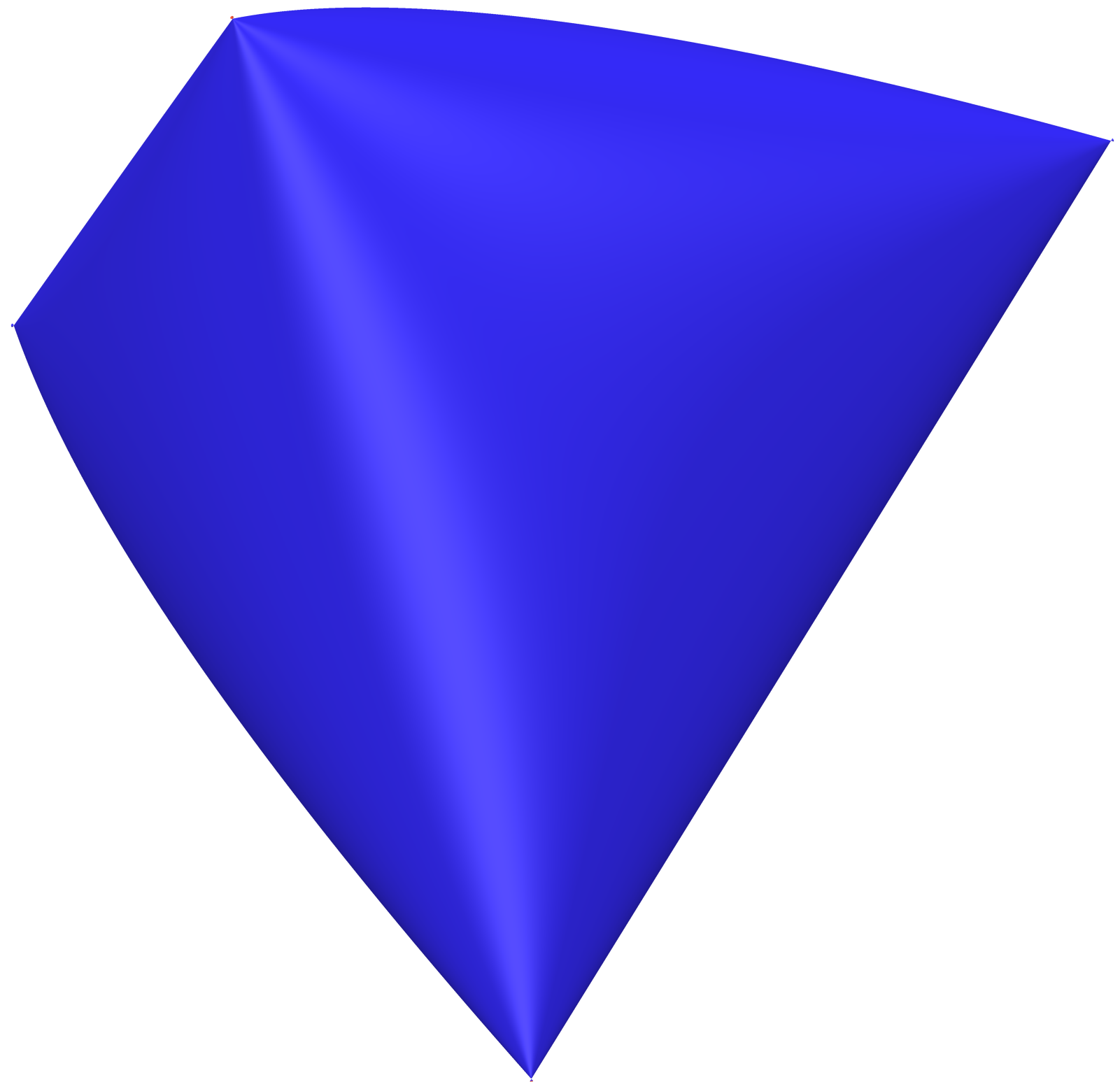
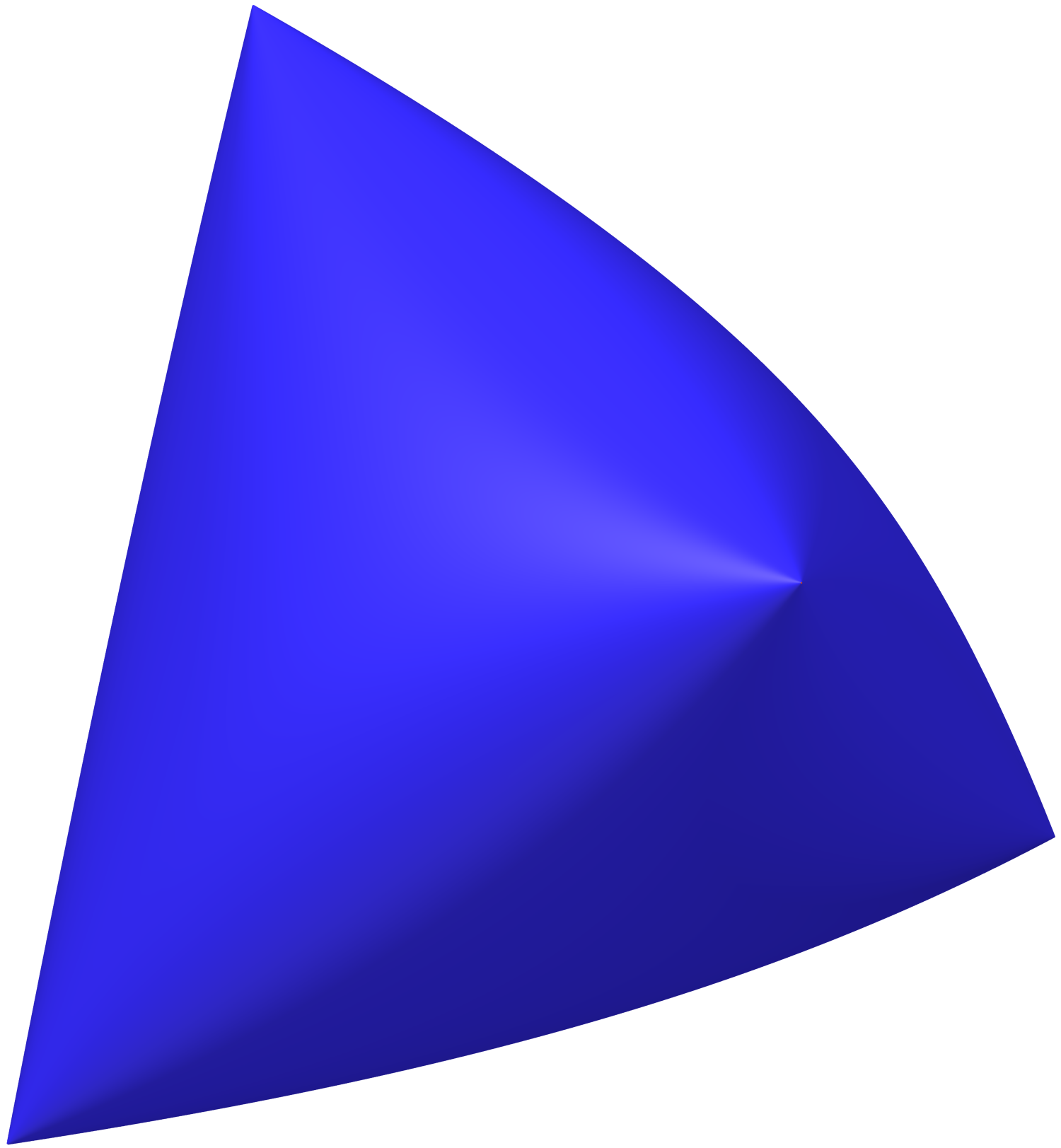
Figure 2.4.1. Two perspectives of ‘The Samosa’

For the quadratic form $g\mathrel{\mathop{:}}=x_{0}^{2}+(x_{1}-x_{2})^{2}\in\partial C$, we have $\varphi(g)=[0:1:1]\in\mathbb{P}(V)$ and

$$\dim(L\cap T_{\varphi(g)})=\dim\operatorname{Span}\bigl{(}x_{0}^{2}+(x_{1}-x_{2})^{2},x_{0}x_{1}-x_{0}x_{2}\bigr{)}=2>1=\dim(L)-\dim(V)\,.$$

This shows that there exist many-faceted spectrahedral cones which do not arise via Lemma 2.1 . $\diamond$

To realize such many-faceted cones within convex algebraic geometry, consider a real projective subscheme $X\subseteq\mathbb{P}^{n}=\operatorname{Proj}(S)$ where $S\mathrel{\mathop{:}}=\mathbb{R}[x_{0},x_{1},\dotsc,x_{n}]$. If $I_{X}$ is the saturated homogeneous ideal defining $X$, then the $\mathbb{Z}$-graded coordinate ring of $X$ is $R\mathrel{\mathop{:}}=S/I_{X}$. For each $j\in\mathbb{Z}$, the graded component $R_{j}$ of degree $j$ is a finite-dimensional real vector space, and we set

$$\operatorname{\Sigma}_{X,2j}\mathrel{\mathop{:}}=\bigl{\{}f\in R_{2j}:\text{there exist $g_{0},g_{1},\dotsc,g_{s}\in R_{j}$ such that $f=g_{0}^{2}+g_{1}^{2}+\dotsb+g_{s}^{2}$}\bigr{\}}\,.$$

Since a nonnegative real number has a square root in $\mathbb{R}$, we see that $\operatorname{\Sigma}_{X,2j}$ is a convex cone in $R_{2j}$. The map $\sigma_{j}\colon\operatorname{Sym}^{2}(R_{j})\to R_{2j}$, induced by multiplication, is surjective. It follows that the cone $\operatorname{\Sigma}_{X,2j}$ is also full-dimensional because the second Veronese embedding of $\mathbb{P}^{n}$ is nondegenerate. Moreover, the dual map $\sigma_{j}^{*}\colon R_{2j}^{*}\to\operatorname{Sym}^{2}(R_{j}^{*})$ is injective and, for all $\ell\in R_{2j}^{*}$, the symmetric form $\sigma_{j}^{*}(\ell)\colon R_{j}\otimes_{\mathbb{R}}R_{j}\to\mathbb{R}$ is given explicitly by $g_{1}\otimes g_{2}\mapsto\ell(g_{1}g_{2})$.

The subsequent proposition consolidates a few fundamental properties of this cone and proves that many-faceted spectrahedral cones are common in convex algebraic geometry. A cone in a real vector space is pointed if it is both closed in the Euclidean topology and contains no lines.

Proposition 2.5.

Fix $j\in\mathbb{N}$. If $X\subseteq\mathbb{P}^{n}$ is a real projective subscheme with $\mathbb{Z}$-graded coordinate ring $R$ such that the map $\eta_{g}\colon R_{j}\to R_{2j}$ defined by $\eta_{g}(f)=fg$ is injective for all nonzero $g\in R_{j}$, then the following are equivalent.

1. The cone $\operatorname{\Sigma}_{X,2j}$ is pointed.

2. No nontrivial sum of squares of forms of degree $j$ equals zero.

3. The points of corank $1$ form a dense subset of $\partial\operatorname{\Sigma}_{X,2j}^{*}$ in the Euclidean topology.

4. The dual $\operatorname{\Sigma}_{X,2j}^{*}$ is a many-faceted spectrahedral cone.

Proof.

(a) $\Rightarrow$ (b): If some nontrivial sum of squares equals zero, then there exist $g_{0},g_{1},\dotsc,g_{s}\in R_{j}$ satisfying $g_{0}^{2}+g_{1}^{2}+\dotsb+g_{s}^{2}=0$. We have $s>0$ because the map $\eta_{g}$ is injective for all nonzero $g\in R_{j}$. Since $g_{0}^{2}=-(g_{1}^{2}+g_{2}^{2}+\dotsb+g_{s}^{2})$, it follows that $\lambda g_{0}^{2}\in\operatorname{\Sigma}_{X,2j}$ for all $\lambda\in\mathbb{R}$ which contradicts the assumption that $\operatorname{\Sigma}_{X,2j}$ contains no lines.

(b) $\Rightarrow$ (a): Fix an inner product on the real vector space $R_{j}$ and let $g\mapsto\|g\|$ denote the associated norm. The spherical section $K\mathrel{\mathop{:}}=\{g^{2}\in R_{2j}:\text{$g\in R_{j}$ satisfies $\|g\|=1$}\}$ is compact because it is the continuous image of a compact set. Moreover, the convex hull of $K$ does not contain $0$ because no nontrivial sum of squares equals zero. Since $\operatorname{\Sigma}_{X,2j}$ is the conical hull of $K$, the cone $\operatorname{\Sigma}_{X,2j}$ is closed. If $\operatorname{\Sigma}_{X,2j}$ contains a line, then there exists a nonzero $f\in R_{2j}$ such that both $f$ and $-f$ lie in $\operatorname{\Sigma}_{X,2j}$. However, it follows that the nontrivial sum $f+(-f)$ equals zero, which contradicts (b).

(a) $\Rightarrow$ (c): Since $\operatorname{\Sigma}_{X,2j}$ is a pointed full-dimensional cone, its dual $\operatorname{\Sigma}_{X,2j}^{*}$ is also a pointed full-dimensional cone. As a consequence, Theorem 2.2.4 in [Schneider] implies that the linear functionals $\ell\in\Sigma_{X,2j}^{*}$ whose normal cone is a single ray form a dense subset of $\partial\Sigma_{X,2j}^{*}$. We claim that every such linear functional $\ell$ has corank one. If $f,g\in R_{j}$ are two nonzero elements lying in the kernel of $\sigma_{j}^{*}(\ell)$, then $f^{2}$ and $g^{2}$ are nonzero elements of the normal cone of $\Sigma_{X,2j}^{*}$ at $\ell$. Because this normal cone is a ray, there exists a positive $\lambda\in\mathbb{R}$ such that $f^{2}=\lambda g^{2}$. Hence, we have $(f+\smash{\sqrt{\lambda}}g)(f-\smash{\sqrt{\lambda}}g)=0$ in $R_{2j}$. By injectivity of multiplication maps, we conclude that $f$ and $g$ are linearly dependent, so $\ell$ has corank $1$ and (c) holds.

(c) $\Rightarrow$ (a): If $\operatorname{\Sigma}_{X,2j}$ is not closed, then the ‘(b) $\Rightarrow$ (a)’ step shows that there is a nontrivial sum of squares from $R_{j}$ equal to zero in $R_{2j}$. In this case, the ‘(a) $\Rightarrow$ (b)’ step demonstrates that $\operatorname{\Sigma}_{X,2j}$ contains a line. Now, if $\operatorname{\Sigma}_{X,2j}$ contains a line, then its dual $\operatorname{\Sigma}_{X,2j}^{*}$ is not full-dimensional. Since the dual map $\sigma_{j}^{*}\colon R_{2j}^{*}\to\operatorname{Sym}^{2}(R_{j}^{*})$ is injective, the linear subspace $\sigma_{j}^{*}(R_{2j}^{*})$ does not intersect the interior of the cone $S_{2}^{+}$ consisting of positive-semidefinite forms in $\operatorname{Sym}^{2}(R_{j}^{*})$. Hence, the image $\sigma_{j}^{*}(\operatorname{\Sigma}_{X,2j}^{*})$ consists of symmetric forms of corank at least $1$. It follows that the boundary consists of symmetric forms of corank at least $2$, which contradicts (c).

(a) $\Leftrightarrow$ (d): Let $V\mathrel{\mathop{:}}=R_{j}$ and let $S_{2}\mathrel{\mathop{:}}=\operatorname{Sym}^{2}(R_{j}^{*})$. For a linear functional $\ell\in\operatorname{\Sigma}_{X,2j}^{*}$, we have $\ell(g^{2})\geqslant 0$ for all $g\in R_{j}$, so the symmetric form $\sigma_{j}^{*}(\ell)$ is positive-semidefinite. Conversely, if $\sigma_{j}^{*}(\ell)$ is positive-semidefinite symmetric form, then we have $\ell(g^{2})\geqslant 0$ for all $g\in R_{j}$. It follows that $\ell(g_{0}^{2}+g_{1}^{2}+\dotsb+g_{s}^{2})=\ell(g_{0}^{2})+\ell(g_{1}^{2})+\dotsb+\ell(g_{s})^{2}\geqslant 0$ for $g_{0},g_{1},\dotsc,g_{s}\in R_{j}$ and $\ell\in\operatorname{\Sigma}_{X,2j}^{*}$. Hence, the map $\sigma_{j}^{*}$ identifies the dual $\operatorname{\Sigma}_{X,2j}^{*}$ with the spectrahedral cone determined by the linear subspace $L\mathrel{\mathop{:}}=\sigma_{j}^{*}(R_{2j}^{*})$ in $S_{2}=\operatorname{Sym}^{2}(R_{j}^{*})$; compare with Lemma 2.1 in [BSV]. Given a nonzero $f\in V$, let $T_{f}\subset S_{2}$ be the linear subspace consisting of the symmetric forms $h\in S_{2}$ such that $f\in\operatorname{Ker}(h)$. As in the proof of Lemma 2.1, we have $\operatorname{codim}T_{f}=\dim V$. The map $\sigma_{j}^{*}$ identifies the linear subspace $L\cap T_{f}$ with the set of linear functionals $\ell\in R_{2j}^{*}$ such that $\ell(fg)=0$ for all $g\in V$. If $\langle f\rangle$ denotes the ideal in $R$ generated by $f$, then it follows that the codimension of $L\cap T_{f}$ in $L$ equals the dimension of $\langle f\rangle_{2j}$. By hypothesis, the map $\eta_{f}\colon R_{j}\to R_{2j}$ is injective, so we obtain $\dim\langle f\rangle_{2j}=\dim R_{j}=\dim V$. Hence, we have $\dim L+\dim T_{f}-\dim L\cap T_{f}=\dim S_{2}$ and the linear subspaces $L$ and $T_{f}$ meet transversely for all nonzero $f\in V$. If $g\in\partial\Sigma_{X,2j}^{*}$ has corank $1$ and $\varepsilon>0$ is sufficiently small, then Lemma 2.1 establishes that the image of $\varphi\colon B_{\varepsilon}(g)\cap\partial\operatorname{\Sigma}_{X,2j}^{*}\to\mathbb{P}(V)$ contains a neighbourhood of $\varphi(g)$. Since ‘(a) $\Leftrightarrow$ (c)’ establishes that $\operatorname{\Sigma}_{X,2j}$ is pointed if and only if the points of corank $1$ form a dense subset of $\partial\operatorname{\Sigma}_{X,2j}^{*}$ in the Euclidean topology, we conclude that $\Sigma_{X,2j}$ is pointed if and only if its dual $\operatorname{\Sigma}_{X,2j}^{*}$ is a many-faceted spectrahedral cone. ∎

Remark 2.6.

The first condition in Proposition 2.5 may be rephrased. A cone $C$ is salient if it does not contain an opposite pair of nonzero vectors, that is $(-C)\cap C\subseteq\{0\}$. In other words, a cone is salient if and only if it contains no lines. Hence, a cone is pointed if it is both closed and salient.

Remark 2.7.

If $\operatorname{\Sigma}_{X,2j}$ is not closed, then the ‘(c) $\Rightarrow$ (a)’ step proves that $\operatorname{\Sigma}_{X,2j}$ contains a line.

We end this section with special cases of Proposition 2.5. A subscheme $X\subseteq\mathbb{P}^{n}$ is a real projective variety if it is a geometrically integral projective scheme over $\mathbb{R}$. Moreover, a real variety $X$ is totally real if the set $X(\mathbb{R})$ of real points is Zariski dense. The most important application of Proposition 2.5 is the following corollary.

Corollary 2.8.

Let $X\subseteq\mathbb{P}^{n}$ be a real projective variety. The cone $\operatorname{\Sigma}_{X,2j}$ is pointed if and only if its dual $\operatorname{\Sigma}_{X,2j}^{*}$ is a many-faceted spectrahedral cone. Furthermore, the cones $\operatorname{\Sigma}_{X,2j}^{*}$ are many-faceted for all $j\in\mathbb{N}$ if and only if $X$ is totally real.

Proof.

Because $X$ is geometrically integral, its coordinate ring $R$ is a domain. Hence, each nonzero element in $R_{j}$ is a nonzerodivisor and the map $\eta_{g}\colon R_{j}\to R_{2j}$ is injective for all nonzero $g\in R_{j}$. By combining this observation with Proposition 2.5, we first conclude that $\operatorname{\Sigma}_{X,2j}$ is pointed if and only if its dual $\operatorname{\Sigma}_{X,2j}^{*}$ is a many-faceted spectrahedral cone. Secondly, $X$ is totally real if and only if, for all $j\in\mathbb{N}$, no nontrivial sum of squares from $R_{j}$ equals zero in $R_{2j}$; compare with Lemma 2.1 in [BSV]. Therefore, the first part together with Proposition 2.5 establishes that the cones $\operatorname{\Sigma}_{X,2j}^{*}$ are many-faceted for every $j\in\mathbb{N}$ if and only if $X$ is totally real. ∎

3. A Bertini Theorem for Separators

In this section, we explore the properties of separating hyperplanes within convex algebraic geometry. Two cones $C_{1}$ and $C_{2}$ in a real vector space are well-separated if there exists a linear functional $\ell$ such that $\ell(v)>0$ for all nonzero $v\in C_{1}$ and $\ell(v)<0$ for all nonzero $v\in C_{2}$. A linear functional $\ell$ with these properties is called a strict separator. If $C_{1}$ and $C_{2}$ are pointed (closed and contain no lines), then being well-separated is equivalent to $C_{1}\cap C_{2}=\{0\}$.

The main result in this section is an analogue of Bertini’s Theorem to convex algebraic geometry. As in Section 2, $X\subseteq\mathbb{P}^{n}$ is a real projective subscheme with $\mathbb{Z}$-graded coordinate ring $R=S/I_{X}$ and $S=\mathbb{R}[x_{0},x_{1},\dotsc,x_{n}]$. Given an element $f\in R_{2j}$, we set $f\cdot\operatorname{\Sigma}_{X,2k}\mathrel{\mathop{:}}=\{fg\in R_{2j+2k}:g\in\operatorname{\Sigma}_{X,2k}\}$. For a nonzero homogeneous polynomial $h\in S$, the associated hypersurface section of $X$ is the subscheme $X^{\prime}\mathrel{\mathop{:}}=X\cap\operatorname{V}(h)\subset\mathbb{P}^{n}$. The $\mathbb{Z}$-graded coordinate ring of $X^{\prime}$ is the quotient $R^{\prime}\mathrel{\mathop{:}}=S/I_{X^{\prime}}$ where $I_{X^{\prime}}$ is the saturated homogeneous ideal $(I_{X}+\langle h\rangle:\langle x_{0},x_{1},\dotsc,x_{n}\rangle^{\infty})$. We write $f^{\prime}\in R^{\prime}_{2j}$ for the canonical image of $f\in R_{2j}$.

Theorem 3.1.

Fix positive integers $j$ and $k$. Let $X\subseteq\mathbb{P}^{n}$ be a real projective subscheme with coordinate ring $R$ such that the map $\eta_{g}\colon R_{j+k}\to R_{2j+2k}$ is injective for all nonzero $g\in R_{j+k}$, and consider a nonzerodivisor $f\in R_{2j}$. If the cones $\operatorname{\Sigma}_{X,2j+2k}$ and $f\cdot\operatorname{\Sigma}_{X,2k}$ are well-separated, then the set of hypersurface sections $X^{\prime}$ of $X$, such that $\operatorname{\Sigma}_{X^{\prime},2j+2k}$ and $f^{\prime}\cdot\operatorname{\Sigma}_{X^{\prime},2k}$ are well-separated, contains a nonempty open subset of $\mathbb{P}(R_{j+k})$ in the Euclidean topology.

Proof.

To begin, we prove that the cones $\operatorname{\Sigma}_{X,2j+2k}$ and $f\cdot\operatorname{\Sigma}_{X,2k}$ are pointed. By hypothesis, $\operatorname{\Sigma}_{X,2j+2k}$ and $f\cdot\operatorname{\Sigma}_{X,2k}$ are well-separated, so neither cone contains a line. Hence, Remark 2.7 shows that $\operatorname{\Sigma}_{X,2j+2k}$ is also closed. As $f$ is a nonzerodivisor, the map $\eta_{f}\colon R_{2k}\to R_{2j+2k}$ is injective, so the cone $\operatorname{\Sigma}_{X,2k}$ is isomorphic to the cone $f\cdot\operatorname{\Sigma}_{X,2k}$. Hence, a second application of Remark 2.7 establishes that both $\operatorname{\Sigma}_{X,2k}$ and $f\cdot\operatorname{\Sigma}_{X,2k}$ are closed.

Now, let $C\mathrel{\mathop{:}}=\operatorname{\Sigma}_{X,2j+2k}^{*}\cap(-f\cdot\operatorname{\Sigma}_{X,2k})^{*}$ be the cone of separators. The cone $C$ is closed and full-dimensional because $\operatorname{\Sigma}_{X,2j+2k}$ and $f\cdot\operatorname{\Sigma}_{X,2k}$ are well-separated. In particular, the boundary of $C$ is not contained in the boundary of $\operatorname{\Sigma}_{X,2j+2k}^{*}$ or the boundary of $(-f\cdot\operatorname{\Sigma}_{X,2k})^{*}$. Since the cone $(-f\cdot\operatorname{\Sigma}_{X,2k})^{*}$ is full-dimensional and

$$D \mathrel{\mathop{:}}=\partial C\setminus\partial(-f\cdot\operatorname{\Sigma}_{X,2k})^{*}$$

$$=\Bigl{(}\bigl{(}\partial(-f\cdot\operatorname{\Sigma}_{X,2k})^{*}\cap\operatorname{\Sigma}_{X,2j+2k}^{*}\bigr{)}\cup\bigl{(}(-f\cdot\operatorname{\Sigma}_{X,2k})^{*}\cap\partial\operatorname{\Sigma}_{X,2j+2k}^{*}\bigr{)}\Bigr{)}\setminus\partial(-f\cdot\operatorname{\Sigma}_{X,2k})^{*}$$

$$=\bigl{(}(-f\cdot\operatorname{\Sigma}_{X,2k})^{*}\setminus\partial(-f\cdot\operatorname{\Sigma}_{X,2k})^{*}\bigr{)}\cap\partial\operatorname{\Sigma}_{X,2j+2k}^{*}\,,$$

it follows that $D$ is a nonempty open subset of $\partial\operatorname{\Sigma}_{X,2j+2k}^{*}$ in the Euclidean topology. Since $\operatorname{\Sigma}_{X,2j+2k}$ is pointed, Proposition 2.5 implies that $\operatorname{\Sigma}_{X,2j+2k}^{*}$ is a many-faceted spectrahedral cone. Hence, the points with corank $1$ form a dense subset of $\partial\operatorname{\Sigma}_{X,2j+2k}^{*}$, so we may choose $g\in D$ with corank $1$. Moreover, for a sufficiently small $\varepsilon>0$, the image of the map $\varphi\colon B_{\varepsilon}(g)\cap D\to\mathbb{P}(R_{j+k})$ contains a neighbourhood $U$ of $\varphi(g)$. Hence, if $\ell\in R_{2j+2k}^{*}$ satisfies $[\varphi(\ell)]\in U$, then there exists $h\in R_{j+k}$ such that $\operatorname{Ker}\sigma_{j+k}^{*}(\ell)=\operatorname{Span}(h)$. Let $X^{\prime}\mathrel{\mathop{:}}=X\cap\operatorname{V}(h)$ denote the corresponding hypersurface section with coordinate ring $R^{\prime}$. Since $\ell^{\prime}$ has corank $1$, the linear functional $\ell\in R_{2j+2k}^{*}$ induces a strict separator $\ell^{\prime}\in(R^{\prime})_{2j+2k}^{*}$ on the cones $\operatorname{\Sigma}_{X^{\prime},2j+2k}$ and $f^{\prime}\cdot\operatorname{\Sigma}_{X^{\prime},2k}$. Therefore, the set of $X^{\prime}$, such that $\operatorname{\Sigma}_{X^{\prime},2j+2k}$ and $f^{\prime}\cdot\operatorname{\Sigma}_{X^{\prime},2k}$ are well-separated, contains the nonempty open subset $U$ of $\mathbb{P}(R_{j+k})$. ∎

To exploit Theorem 3.1, we also need to understand the properties of strict separators on zero-dimensional schemes. As we will see, the existence of strict separators imposes nontrivial constrains on a set of points. For a real projective scheme $X\subseteq\mathbb{P}^{n}$ with homogeneous coordinate ring $R$, the Hilbert function $\operatorname{h}_{X}\colon\mathbb{Z}\to\mathbb{Z}$ is defined by $\operatorname{h}_{X}(j)\mathrel{\mathop{:}}=\dim_{\mathbb{R}}R_{j}$. Following Section 3.1 in [HarrisMontreal] or Section 2 in [HarrisGenus], a set of points $X\subseteq\mathbb{P}^{n}$, that is a zero-dimensional reduced subscheme, has the uniform position property if the Hilbert function of a subset of $X$ depends only on the cardinality of the subset.

The concluding proposition of this section shows that the existence of certain positive linear functionals on a set of points imposes constraints on its Hilbert function.

Proposition 3.2.

Fix positive integers $j$ and $k$, and let $X\subseteq\mathbb{P}^{n}$ be a set of at least two points with the uniform position property.

1. Suppose that $X$ has no real points. If there exists a linear functional $\ell\in R_{2k}^{*}$ that is positive on the nonzero elements in $\operatorname{\Sigma}_{X,2k}$, then we have $\operatorname{h}_{X}(k)\leqslant\bigl{\lceil}\frac{1}{2}\operatorname{h}_{X}(2k)\bigr{\rceil}$.

2. Suppose that $f\in R_{2j}$ is positive on $X(\mathbb{R})$ and does not vanish at any point in $X(\mathbb{C})$. If there exists a linear functional $\ell\in R_{2j+2k}^{*}$ that is a strict separator for $\operatorname{\Sigma}_{X,2j+2k}$ and $f\cdot\operatorname{\Sigma}_{X,2k}$, then we have $\operatorname{h}_{X}(k)+\operatorname{h}_{X}(j+k)\leqslant\operatorname{h}_{X}(2j+2k)$.

Proof.

We begin with an analysis of the symmetric forms arising from point evaluations. Let $Z\subseteq X$ be a subset consisting of $e$ distinct real points and $m$ complex conjugate pairs. Choose affine representatives $\tilde{p}_{1},\tilde{p}_{2},\dotsc,\tilde{p}_{e}\in\mathbb{A}^{n+1}(\mathbb{R})$ for points in $Z(\mathbb{R})$, and choose affine representatives $\tilde{a}_{1}\pm\tilde{b}_{1}\sqrt{-1},\tilde{a}_{2}\pm\tilde{b}_{2}\sqrt{-1},\dotsc,\tilde{a}_{m}\pm\tilde{b}_{m}\sqrt{-1}\in\mathbb{A}^{n+1}(\mathbb{R})$ where $\tilde{a}_{j},\tilde{b}_{j}\in\mathbb{A}^{n+1}(\mathbb{R})$ for the complex conjugate pairs in $Z(\mathbb{C})$. For any $p\in X(\mathbb{R})$ and any $k\in\mathbb{N}$, evaluation at an affine representative $\tilde{p}\in\mathbb{A}^{n+1}(\mathbb{R})$ determines the linear functional $\tilde{p}^{*}\in R_{2k}^{*}$. Any linear functional $\ell\in R_{2k}^{*}$ lying in the span of these point evaluations can be written as

$$\ell =\sum_{i=1}^{e}\kappa_{i}\tilde{p}_{i}^{*}+\sum_{j=1}^{m}\bigl{(}(\lambda_{j}+\mu_{j}\sqrt{-1})(\tilde{a}_{j}+\tilde{b}_{j}\sqrt{-1})^{*}+(\lambda_{j}-\mu_{j}\sqrt{-1})(\tilde{a}_{j}-\tilde{b}_{j}\sqrt{-1})^{*}\bigr{)}$$

where $\kappa_{i},\lambda_{j},\mu_{j}\in\mathbb{R}$ for $1\leqslant i\leqslant e$ and $1\leqslant j\leqslant m$. It follows that

$$\sigma_{k}^{*}(\ell)=\sum_{i=1}^{e}\kappa_{i}(\tilde{p}_{i}^{*})^{2}+\sum_{j=1}^{m}\lambda_{j}\bigl{(}(\tilde{a}_{j}^{*})^{2}-(\tilde{b}_{j}^{*})^{2}\bigr{)}-2\mu_{j}(\tilde{a}_{j}^{*})(\tilde{b}_{j}^{*})\in\operatorname{Sym}^{2}(R_{k}^{*})\,.$$

The eigenvalues for the symmetric matrix

$$\begin{bmatrix}\phantom{-}\lambda_{j}&-\mu_{j}\\ -\mu_{j}&-\lambda_{j}\\ \end{bmatrix}$$

are $\pm\sqrt{\smash[b]{\lambda_{j}^{2}+\mu_{j}^{2}}}$, so the number of positive eigenvalues for $\sigma_{k}^{*}(\ell)$ is at most the number $e_{+}$ of positive $\kappa_{i}$ plus the number $m^{\prime}$ of nonzero $\lambda_{j}^{2}+\mu_{j}^{2}$. Similarly, the number of negative eigenvalues for $\sigma_{k}^{*}(\ell)$ is at most the number $e_{-}$ of negative $\kappa_{i}$ plus the number $m^{\prime}$ of nonzero $\lambda_{j}^{2}+\mu_{j}^{2}$. Hence, if $\sigma_{k}^{*}(\ell)$ is positive-definite, then we have $\operatorname{h}_{X}(k)=\dim R_{k}^{*}\leqslant e_{+}+m^{\prime}$.

Using this analysis, we prove (i). Assume that $\ell\in R_{2k}^{*}$ is positive on the nonzero elements in $\operatorname{\Sigma}_{X,2k}$. A form in $R_{2k}^{*}$ is zero if and only if it is annihilated by $\tilde{p}^{*}\in R_{2k}^{*}$ for all points $p\in X(\mathbb{C})$. Hence, every linear functional in $R_{2k}^{*}$ can be written as a $\mathbb{C}$-linear combinations of such point evaluations. The evaluations at the points in any subset $X$, with cardinality at least $\operatorname{h}_{X}(2k)$, span $R_{2k}^{*}$ because $X$ has the uniform position property. As $X$ is a set of points, the value of Hilbert function $\operatorname{h}_{X}(k)$ is at most the number of points. Since $X(\mathbb{R})=\varnothing$, we may choose $m$ conjugate pairs of points in $X(\mathbb{C})$ with $m\mathrel{\mathop{:}}=\bigl{\lceil}\tfrac{1}{2}\operatorname{h}_{X}(2k)\bigr{\rceil}$; in particular, we have $e=0$. Since $\sigma_{k}^{*}(\ell)$ is positive-definite, the first paragraph shows that $\operatorname{h}_{X}(k)\leqslant m^{\prime}\leqslant m=\bigl{\lceil}\tfrac{1}{2}\operatorname{h}_{X}(2k)\bigr{\rceil}$ as required.

We next examine the symmetric forms induced by the element $f\in R_{2k}$. Given $\ell\in R_{2k+2k}^{*}$, the linear functional $\ell^{\prime}\in R_{2k}^{*}$ is defined by $\ell^{\prime}(g)\mathrel{\mathop{:}}=\ell(fg)$ for all $g\in R_{2k}$. When $\ell\in R_{2j+2k}^{*}$ lies in the span of the point evaluations for $Z$, the expression for $\ell^{\prime}$ as a linear combination of the point evaluations has the same number of positive, negative, and nonzero coefficients as $\ell$ because $f\in R_{2j}$ is positive on $X(\mathbb{R})$ and does not vanish at any points in $X(\mathbb{C})$. Hence, if $\sigma_{k}^{*}(\ell^{\prime})$ is negative-definite, then the first paragraph implies that $\operatorname{h}_{X}(k)=\dim R_{k}^{*}\leqslant e_{-}+m^{\prime}$.

Lastly, we establish (ii). Assume that $\ell\in R_{2j+2k}^{*}$ is a strict separator for $\operatorname{\Sigma}_{X,2j+2k}$ and $f\cdot\operatorname{\Sigma}_{X,2k}$. As in the second paragraph, we may choose a subset of $X$ such that the point evaluations span $R_{2j+2k}^{*}$. Suppose that there exists a conjugate-invariant basis of $R_{2j+2k}^{*}$ consisting of point evaluations at $e$ distinct real points and $m$ complex conjugate pairs. Since $\sigma_{k}^{*}(\ell^{\prime})$ is negative-definite and $\sigma_{j+k}^{*}(\ell)$ is positive-definite, the first and third paragraphs combine to show that

$$\operatorname{h}_{X}(k)+\operatorname{h}_{X}(j+k)\leqslant(e_{-}+m^{\prime})+(e_{+}+m^{\prime})\leqslant e+2m=\operatorname{h}_{X}(2j+2k)\,.$$

On the other hand, if no subset of $X$ yields a conjugate-invariant basis of $R_{2j+2k}^{*}$, then there are $m\mathrel{\mathop{:}}=\bigl{\lceil}\tfrac{1}{2}\operatorname{h}_{X}(2j+2k)\bigr{\rceil}$ conjugate pairs of points in $X(\mathbb{C})$ that span $R_{2j+2k}^{*}$ and we have $e=0$. Hence, we obtain $\operatorname{h}_{X}(j+k)\leqslant m$, $2\operatorname{h}_{X}(j+k)\leqslant 2m=\operatorname{h}_{X}(2j+2k)+1$, and $2\operatorname{h}_{X}(j+k)-1\leqslant\operatorname{h}_{X}(2j+2k)$. With the goal of finding a contradiction, assume that $\operatorname{h}_{X}(k)+\operatorname{h}_{X}(j+k)>\operatorname{h}_{X}(2j+2k)$. It follows that $\operatorname{h}_{X}(k)+1>\operatorname{h}_{X}(j+k)$. The Hilbert function of a set of points is strictly increasing until it stabilizes at the number points, so we deduce that $\operatorname{h}_{X}(k)=\operatorname{h}_{X}(j+k)=\operatorname{h}_{X}(2j+2k)$. Hence, the inequality $2\operatorname{h}_{X}(j+k)\leqslant\operatorname{h}_{X}(2j+2k)+1$ implies that $\operatorname{h}_{X}(j+k)=1$. However, this contradicts the hypothesis that $X$ has at least two points. Therefore, we conclude that $\operatorname{h}_{X}(k)+\operatorname{h}_{X}(j+k)\leqslant\operatorname{h}_{X}(2j+2k)$. ∎

4. Upper Bounds for Sum-of-Squares Multipliers

This section establishes an upper bound on the minimal degree of a sum-of-squares multiplier. These geometric degree bounds for the existence of multipliers prove the first halves of our main theorems. After a preparatory lemma, Theorem 4.3 describes the general result for curves and is followed by several corollaries and valuable examples. The same approach is then applied to higher-dimensional varieties to obtain the general Theorem 4.13. The ensuing examples illustrate the applicability of this theorem.

Throughout this section, we work with a real projective subscheme $X\subseteq\mathbb{P}^{n}$ with $\mathbb{Z}$-graded coordinate ring $R=S/I_{X}$. The sign of an element $f\in R_{2j}$ at a real point $p\in X(\mathbb{R})$ is defined to be $\operatorname{sgn}_{p}(f)\mathrel{\mathop{:}}=\operatorname{sgn}\bigl{(}\tilde{f}(\tilde{p})\bigr{)}\in\{-1,0,1\}$, where the polynomial $\tilde{f}\in S_{2j}$ maps to $f$ and the nonzero real point $\tilde{p}\in\mathbb{A}^{n+1}(\mathbb{R})$ maps to $p$ under the canonical quotient maps. Since $p\in X(\mathbb{R})$, the real number $\tilde{f}(\tilde{p})$ is independent of the choice of $\tilde{f}$. Similarly, the choice of affine representative $\tilde{p}$ is determined up to a nonzero real number and the degree of $f$ is even, so the value of $\tilde{f}(\tilde{p})$ is determined up to the square of a nonzero real number. Hence, the sign of $f\in R_{2j}$ at $p\in X(\mathbb{R})$ is well-defined. We simply write $f(p)\geqslant 0$ for $\operatorname{sgn}_{p}(f)\geqslant 0$. The subset $\operatorname{P}_{X,2j}\mathrel{\mathop{:}}=\{f\in R_{2j}:\text{$f(p)\geqslant 0$ for all $p\in X(\mathbb{R})$}\}$ forms a pointed full-dimensional convex cone in $R_{2j}$; see Lemma 2.1 in [BSV].

As our initial focus, a curve $X\subseteq\mathbb{P}^{n}$ is a one-dimensional projective variety. Following Chapter 2 of [Migliore], the deficiency module (also known as the Hartshorne-Rao module) of $X$ is the $\mathbb{Z}$-graded $S$-module $M_{X}\mathrel{\mathop{:}}=\bigoplus_{i\in\mathbb{Z}}H^{1}\bigl{(}\mathbb{P}^{n},\mathcal{I}_{X}(i)\bigr{)}$. A homogeneous polynomial $h\in S=\mathbb{R}[x_{0},x_{1},\dotsc,x_{n}]$ determines the $\mathbb{Z}$-graded submodule $\operatorname{Ann}_{M_{X}}(h)\mathrel{\mathop{:}}=(0:_{M(X)}h)=\{f\in M_{X}:fh=0\}$ of the deficiency module $M_{X}$. The next lemma (cf. Proposition 2.1.2 in [Migliore]) shows that this submodule measures the failure of the ideal $I_{X}+\langle h\rangle$ to be saturated.

Lemma 4.1.

Fix a positive integer $j$ and a nonnegative integer $k$. Let $X\subseteq\mathbb{P}^{n}$ be a curve. If $h\in S_{k}$ does not belong to the ideal $I_{X}$ and $X^{\prime}\mathrel{\mathop{:}}=X\cap\operatorname{V}(h)$ is the associated hypersurface section of $X$, then we have $\operatorname{Ann}_{M_{X}}(h)_{j-k}=0$ if and only if $(I_{X^{\prime}})_{j}=(I_{X}+\langle h\rangle)_{j}$.

Proof.

By definition, the submodule $\operatorname{Ann}_{M_{X}}(h)$ fits into the exact sequence

$$0\longrightarrow\bigl{(}\operatorname{Ann}_{M_{X}}(h)\bigr{)}(-k)\longrightarrow M_{X}(-k)\xrightarrow{\;\;\cdot h\;\;}M_{X}\,.$$

Sheafifying the canonical short exact sequence $0\longrightarrow I_{X}\cap\langle h\rangle\longrightarrow I_{X}\oplus\langle h\rangle\longrightarrow I_{X}+\langle h\rangle\longrightarrow 0$ and taking cohomology of appropriate twists produces the long exact sequence

$$0\longrightarrow I_{X}(-k)\xrightarrow{\;\;\left[\begin{smallmatrix}h\\ h\end{smallmatrix}\right]\;\;}I_{X}\oplus\langle h\rangle\longrightarrow I_{X^{\prime}}\longrightarrow M_{X}(-k)\xrightarrow{\;\;\cdot h\;\;}M_{X}\,.$$

Breaking this long exact sequence into short exact sequences, we obtain

$$0\longrightarrow I_{X}+\langle h\rangle\longrightarrow I_{X^{\prime}}\longrightarrow\bigl{(}\operatorname{Ann}_{M_{X}}(h)\bigr{)}(-k)\longrightarrow 0\,.$$

Thus, we have $\bigl{(}\operatorname{Ann}_{M_{X}}(h)\bigr{)}(-k)\cong I_{X^{\prime}}/(I_{X}+\langle h\rangle)$ and the required equivalence follows. ∎

As a consequence of Lemma 4.1, we see that some natural geometric conditions imply that the ideal $I_{X}+\langle h\rangle$ is saturated.

Remark 4.2.

A curve $X$ is projectively normal if and only if $M_{X}=0$. With this hypothesis, Lemma 4.1 implies that we have $(I_{X^{\prime}})_{j}=(I_{X}+\langle h\rangle)_{j}$ for all $j\in\mathbb{Z}$. In particular, if $X$ is arithmetically Cohen–Macaulay, then the ideal $I_{X}+\langle h\rangle$ is saturated.

The next result is the general form of our degree bound for the existence of sum-of-squares multipliers on curves.

Theorem 4.3.

Fix a positive integer $j$ and a nonnegative integer $k$. Let $X\subseteq\mathbb{P}^{n}$ be a totally-real curve such that $H^{1}\bigl{(}\mathbb{P}^{n},\mathcal{I}_{X}(j+k)\bigr{)}=0$ and $\operatorname{h}_{X}(2j+2k)<2\operatorname{h}_{X}(j+k)+\operatorname{h}_{X}(k)-1$. For all $f\in\operatorname{P}_{X,2j}$, there exists a nonzero $g\in\operatorname{\Sigma}_{X,2k}$ such that $fg\in\operatorname{\Sigma}_{X,2j+2k}$.

Proof.

We start by reinterpreting the non-existence of a suitable multiplier $g\in\operatorname{\Sigma}_{X,2k}$ as the existence of a strict separator between appropriate cones. Corollary 2.8 implies that the cones $\operatorname{\Sigma}_{X,2j+2k}$ and $\operatorname{\Sigma}_{X,2k}$ are pointed. If $f=0$, then the conclusion is trivial, so we may assume that $f$ is nonzero. It follows that $f$ is a nonzerodivisor because $X$ is integral. Since the map $\eta_{f}\colon R_{2k}\to R_{2j+2k}$ is injective, the pointed cone $\operatorname{\Sigma}_{X,2k}$ is isomorphic to the cone $f\cdot\operatorname{\Sigma}_{X,2k}$. Hence, the non-existence of a nonzero $g\in\operatorname{\Sigma}_{X,2k}$ such that $fg\in\operatorname{\Sigma}_{X,2j+2k}$ is equivalent to saying that the cones $\operatorname{\Sigma}_{X,2j+2k}$ and $f\cdot\operatorname{\Sigma}_{X,2k}$ are well-separated.

To complete the proof, we reduce to the case of points by using new and old Bertini Theorems. Our convex variant, Theorem 3.1, implies that the set of homogeneous polynomials $h\in S_{j+k}$, such that $h\not\in I_{X}$, $X^{\prime}\mathrel{\mathop{:}}=X\cap\operatorname{V}(h)\subset\mathbb{P}^{n}$, and the cones $\operatorname{\Sigma}_{X^{\prime},2j+2k}$ and $f^{\prime}\cdot\operatorname{\Sigma}_{X^{\prime},2k}$ are well-separated, contains a nonempty Euclidean open subset $U_{1}\subseteq\mathbb{P}(R_{j+k})$. The classic version of Bertini’s Theorem (see Théorème 6.3 in [J]) shows that there is a nonempty Zariski open subset $U_{2}\subseteq\mathbb{P}(R_{j+k})$ such that, for all $[h]\in U_{2}$, the hypersurface section $X^{\prime}$ is a reduced set of points and $f$ does not vanish at any point in $X^{\prime}$. Moreover, our hypothesis that $(M_{X})_{j+k}=0$ combined with Lemma 4.1 establishes that there exists another nonempty Zariski open subset $U_{3}\subseteq\mathbb{P}(R_{j+k})$ such that, for all $[h]\in U_{3}$, we have $(I_{X^{\prime}})_{2j+2k}=(I_{X}+\langle h\rangle)_{2j+2k}$, which implies that $\operatorname{h}_{X^{\prime}}(2j+2k)=\operatorname{h}_{X}(2j+2k)-\operatorname{h}_{X}(j+k)$. The triple intersection $U_{1}\cap U_{2}\cap U_{3}$ is nonempty, so Proposition 3.2 (ii) yields the inequality $\operatorname{h}_{X^{\prime}}(k)+\operatorname{h}_{X^{\prime}}(j+k)\leqslant\operatorname{h}_{X^{\prime}}(2j+2k)$. By construction, we have $\operatorname{h}_{X^{\prime}}(j+k)\leqslant\operatorname{h}_{X}(j+k)-1$ and $\operatorname{h}_{X^{\prime}}(i)\leqslant\operatorname{h}_{X}(i)$ for all $i<j+k$. Therefore, we conclude that $\operatorname{h}_{X}(k)+2\operatorname{h}_{X}(j+k)-1\leqslant\operatorname{h}_{X}(2j+2k)$ when the cones $\operatorname{\Sigma}_{X,2j+2k}$ and $f\cdot\operatorname{\Sigma}_{X,2k}$ are well-separated. ∎

The hypothesis in Theorem 4.3 may be recast using alternative numerical invariants. With this in mind, set $\operatorname{e}_{i}(X)\mathrel{\mathop{:}}=\max\{i\in\mathbb{Z}:H^{i}\bigl{(}\mathbb{P}^{n},\mathcal{I}_{X}(i)\bigr{)}\neq 0\}$, so that the Castelnuovo–Mumford regularity of $\mathcal{I}_{X}$ equals $\max\{\operatorname{e}_{i}(X)+i:i\in\mathbb{Z}\}$; compare with Theorem 4.3 in [EisSyz].

Corollary 4.4.

Fix a positive integer $j$ and a nonnegative integer $k$. Let $X\subseteq\mathbb{P}^{n}$ be a totally-real curve of degree $d$ and arithmetic genus $p_{\text{a}}$, and assume that

$$k\geqslant\max\bigl{\{}\operatorname{e}_{1}(X)+1,\tfrac{1}{2}\operatorname{e}_{2}(X)+\tfrac{1}{2}-j,\tfrac{2p_{\text{a}}}{d}\bigr{\}}\,.$$

For all $f\in\operatorname{P}_{X,2j}$, there exists a nonzero $g\in\operatorname{\Sigma}_{X,2k}$ such that $fg\in\operatorname{\Sigma}_{X,2j+2k}$.

Proof.

When $j+k\geqslant\operatorname{e}_{1}(X)+1$, we have $H^{1}\bigl{(}\mathbb{P}^{,}\mathcal{I}_{X}(j+k)\bigr{)}=(M_{X})_{j+k}=0$; compare with Remark 4.2. The Hilbert polynomial of $X$ equals $\operatorname{p}_{X}(i)=di+(1-p_{\text{a}})$ and satisfies

$$\operatorname{h}_{X}(i)-\operatorname{p}_{X}(i)=\dim H^{2}\bigl{(}\mathbb{P}^{2},\mathcal{I}_{X}(i)\bigr{)}-\dim H^{1}\bigl{(}\mathbb{P}^{2},\mathcal{I}_{X}(i)\bigr{)}\,,$$

so we see that $\operatorname{h}_{X}(i)=\operatorname{p}_{X}(i)$ for all $i>\max\{\operatorname{e}_{1}(X),\operatorname{e}_{2}(X)\}$ and $\operatorname{h}_{X}(i)\geqslant\operatorname{p}_{X}(i)$ for all $i>\operatorname{e}_{1}(X)$. Hence, if $k\geqslant\operatorname{e}_{1}(X)+1$ and $2j+2k\geqslant\operatorname{e}_{2}(X)+1$, then the inequality $k\geqslant\frac{2p_{\text{a}}}{d}$ or $k>\frac{2p_{\text{a}}-1}{d}$ is equivalently to $\operatorname{p}_{X}(2j+2k)<2\operatorname{p}_{X}(j+k)+\operatorname{p}_{X}(k)-1$ and $\operatorname{h}_{X}(2j+2k)<2\operatorname{h}_{X}(j+k)+\operatorname{h}_{X}(k)-1$. Therefore, Theorem 4.3 establishes the corollary. ∎

For a second version, set $\operatorname{r}(X)\mathrel{\mathop{:}}=\min\{j\in\mathbb{Z}:\text{$\operatorname{h}_{X}(i)=\operatorname{p}_{X}(i)$ for all $i\geqslant j$}\}$ where $\operatorname{p}_{X}(i)$ denotes the Hilbert polynomial of $X$. This numerical invariant is sometimes called the Hilbert regularity of $X$ or the index of regularity for $X$. A curve $X\subset\mathbb{P}^{n}$ is nondegenerate if it is not contained in a hyperplane.

Corollary 4.5.

Fix a positive integer $j$ and a nonnegative integer $k$. Let $X\subset\mathbb{P}^{n}$ be a nondegenerate totally-real curve of degree $d$ and arithmetic genus $p_{\text{a}}$, and assume that $k\geqslant\max\bigl{\{}\operatorname{r}(X),\frac{2p_{\text{a}}}{d}\bigr{\}}$. For all $f\in\operatorname{P}_{X,2j}$, there is a nonzero $g\in\operatorname{\Sigma}_{X,2k}$ such that $fg\in\operatorname{\Sigma}_{X,2j+2k}$.

Proof.

The inequalities $k\geqslant\operatorname{r}(X)$ and $k\geqslant\frac{2p_{\text{a}}}{d}$ yield $\operatorname{h}_{X}(j+k)=\operatorname{p}_{X}(j+k)=d(j+k)+(1-p_{\text{a}})$ and $d(j+k)-p_{\text{a}}=dj+dk-p_{\text{a}}\geqslant dj+p_{\text{a}}\geqslant 2$ respectively. By hypothesis, the line bundle $\mathcal{O}_{X}(1)$ is very ample and $j+k\geqslant 1$, so the complete linear series $|\mathcal{O}_{X}(j+k)|$ defines a closed immersion $\varphi\colon X\to\mathbb{P}^{d(j+k)-p_{\text{a}}}$. If $Y\mathrel{\mathop{:}}=\varphi(X)$, then a generic hyperplane section $Y^{\prime}$ of the curve $Y$ consists of $d(j+k)$ points, any $d(j+k)-p_{\text{a}}$ of which are linearly independent; see the General Position Theorem on page 109 in [ACGH]. Employing the inequality $k\geqslant\frac{2p_{\text{a}}}{d}$ as second time, we observe that $d(j+k)<d(j+k)+(dk-2p_{\text{a}})+dj-1=2\bigl{(}d(j+k)-p_{\text{a}}-1\bigr{)}+1$. Hence, the Lemma on page 115 in [ACGH] establishes that the points in $Y^{\prime}$ impose independent conditions on homogeneous polynomials of degree $2$, and Corollary 4.7 in [EisSyz] shows that $\mathcal{I}_{Y^{\prime}}$ is $2$-regular. In particular, we obtain $H^{1}\bigl{(}\mathbb{P}^{d(j+k)-p_{\text{a}}},\mathcal{I}_{Y^{\prime}}(1)\bigr{)}=0$. Since $X$ is nondegenerate, the curve $Y$ is also nondegenerate and we also have $H^{1}(\mathbb{P}^{d(j+k)-p_{\text{a}}},\mathcal{I}_{Y})=0$. The long exact sequence in cohomology arising from the short exact sequence $0\longrightarrow\mathcal{I}_{Y}(-1)\longrightarrow\mathcal{I}_{Y}\longrightarrow\mathcal{I}_{Y^{\prime}}\longrightarrow 0$ implies that $0=H^{1}\bigl{(}\mathbb{P}^{d(j+k)-p_{\text{a}}},\mathcal{I}_{Y}(1)\bigr{)}=H^{1}\bigl{(}\mathbb{P}^{n},\mathcal{I}_{X}(j+k)\bigr{)}$. Since $k\geqslant\operatorname{r}(X)$, we have $\operatorname{h}_{X}(i)=\operatorname{p}_{X}(i)$ for all $i\geqslant k$ and the inequality $k\geqslant\frac{2p_{\text{a}}}{d}$ is equivalent to $\operatorname{h}_{X}(2j+2k)<2\operatorname{h}_{X}(j+k)+\operatorname{h}_{X}(k)-1$, as in the proof of Corollary 4.4. Therefore, Theorem 4.3 establishes the corollary. ∎

We illustrate these corollaries for two classic families of curves.

Example 4.6 (Complete intersection curves).

Consider a totally-real complete intersection curve $X\subseteq\mathbb{P}^{n}$ cut out by forms of degree $d_{1},d_{2},\dotsc,d_{n-1}$ for $1\leqslant i\leqslant n-1$ where at least one $d_{i}$ is greater than $1$. This curve is arithmetically Cohen–Macaulay, so $\operatorname{e}_{1}(X)=-\infty$; compare with Remark 4.2. By breaking the minimal free resolution of $\mathcal{I}_{X}$ (which is a Koszul complex) into short exact sequences and knowing the cohomology of line bundles on projective space, we deduce that $\operatorname{r}(X)=\operatorname{e}_{2}(X)=d_{1}+d_{2}+\dotsb+d_{n-1}-n-1$. As in Example 1.5.1 in [Migliore], the degree of $X$ is $d_{1}d_{2}\dotsb d_{n-1}$ and the arithmetic genus is $\tfrac{1}{2}(d_{1}d_{2}\dotsb d_{n-1})(d_{1}+d_{2}+\dotsb+d_{n-1}-n-1)+1$. Assuming that $k\geqslant d_{1}+d_{2}+\dotsb+d_{n-1}-n$, Corollary 4.4 or Corollary 4.5 establish that, for all $f\in\operatorname{P}_{X,2j}$, there exists a nonzero $g\in\operatorname{\Sigma}_{X,2k}$ such that $fg\in\operatorname{\Sigma}_{X,2j+2k}$. $\diamond$

Example 4.7 (Planar curves).

If $X\subset\mathbb{P}^{2}$ is a planar curve of degree $d$ at least $2$ and $k\geqslant d-2$, then Example 4.6 implies that, for all $f\in\operatorname{P}_{X,2j}$, there is a nonzero $g\in\operatorname{\Sigma}_{X,2k}$ such that $fg\in\operatorname{\Sigma}_{X,2j+2k}$. $\diamond$

Although Example 5.3 shows that this degree bound from Corollary 4.5 is sharp on some planar curves, the next example demonstrates that this is not always the case. Moreover, it illustrates how our techniques yield sharper bounds when the convex algebraic geometry of the underlying variety is well understood.

Example 4.8 (Non-optimality for planar curves).

Let $X\subset\mathbb{P}^{2}$ be a rational quartic curve with a real parametrization and a real triple point. For instance, the curve $X$ could be the image of the map $[x_{0}:x_{1}]\mapsto[x_{0}^{2}x_{1}(x_{0}-x_{1}):x_{0}x_{1}^{2}(x_{0}-x_{1}):x_{0}^{4}+x_{1}^{4}]$ where $[1:0],[0:1],[1:1]\in\mathbb{P}^{1}$ are all sent to $[0:0:1]\in\mathbb{P}^{2}$; this curve has degree $4$, arithmetic genus $3$, and $\operatorname{r}(X)=2$. We claim that, for all $f\in\operatorname{P}_{X,2}$, there exists a nonzero $g\in\operatorname{\Sigma}_{X,2}$ such that $fg\in\operatorname{\Sigma}_{X,4}$.

We first reduce the claim to showing that a generic linear functional $\ell\in R_{4}^{*}$ can be written as conjugate-invariant linear combination of at most $8$ point evaluations on $X(\mathbb{C})$. If the claim is false, then there exists a linear functional $\ell\in R_{4}^{*}$ that strictly separates $\operatorname{\Sigma}_{X,4}$ and $f\cdot\operatorname{\Sigma}_{X,2}$. We may assume that $\ell\in R_{4}^{*}$ is a generic linear functional because $\operatorname{\Sigma}_{X,4}$ and $f\cdot\operatorname{\Sigma}_{X,2}$ are pointed cones. Since $\operatorname{h}_{X}(2)=6$ and $\operatorname{h}_{X}(1)=3$, the affine hulls of $\operatorname{\Sigma}_{X,4}$ and $f\cdot\operatorname{\Sigma}_{X,2}$ have dimension $6$ and $3$ respectively. As analysis of symmetric forms arising from point evaluations appearing in the proof of Proposition 3.2 indicates, the number of real point evaluations with positive coefficients plus the number of pairs of complex point evaluations is at least $6$ and the number of real point evaluations with negative coefficients plus the number of pairs of complex point evaluations is at least $3$. However, if $\ell\in R_{4}^{*}$ is a conjugate-invariant linear combination of at most $8$ point evaluations, then we obtain a contradiction.

It remains to show that a generic linear functional $\ell\in R_{4}^{*}$ is a conjugate-invariant linear combination of at most $8$ point evaluations on $X(\mathbb{C})$. The curve $X$ is a projection of the rational normal quartic curve $\breve{X}\subset\mathbb{P}^{4}$. It follows that there is a linear surjection $\rho\colon\breve{R}_{4}^{*}\to R_{4}^{*}$ sending point evaluations on $\breve{X}$ to point evaluations on $X$. Hence, it suffices to prove that, for a generic $\ell\in R_{4}^{*}$, there exists a linear functional $\breve{\ell}\in\rho^{-1}(\ell)$ that is a conjugate-invariant linear combination of at most $8$ points evaluations on $\breve{X}(\mathbb{C})$.

By construction, the $\mathbb{R}$-vector space $\breve{R}_{4}$ is isomorphic to $\mathbb{R}[x_{0},x_{1}]_{16}$. Thus, a generic linear functional $\breve{\ell}\in\breve{R}_{4}$ can be written as a conjugate-invariant linear combination of at most $9$ point evaluations; see Lemma 1.33 in [IK]. Moreover, $\breve{\ell}\in\breve{R}_{4}$ can be written as a conjugate-invariant linear combination of $9$ point evaluations if and only if the corresponding $(8\times 8)$-catelecticant matrix is invertible; see Theorem 1.44 or the second paragraph on page 28 in [IK]. A general element in $\breve{R}_{4}$, for which the corresponding $(8\times 8)$-catelecticant matrix is not invertible, is a conjugate-invariant linear combination of $8$ point evaluations. Hence, it is enough to show that there exists $\breve{\ell}\in\rho^{-1}(\ell)$ for which the corresponding catelecticant is not invertible. Since three points of $\breve{X}$ are mapped to the same point in $X$, there exists a linear functional $\breve{\ell}^{\prime}\in\rho^{-1}(0)$ such that the corresponding $(8\times 8)$-catelecticant matrix has rank $3$; compare with Theorem 1.43 in [IK]. Choose an arbitrary linear functional $\breve{\ell}^{\prime\prime}\in\rho^{-1}(\ell)$ and consider the pencil $\breve{\ell}^{\prime\prime}+\lambda\breve{\ell}^{\prime}$ where $\lambda\in\mathbb{R}$. The determinant of the $(8\times 8)$-catelecticant matrix corresponding to $\breve{\ell}^{\prime\prime}+\lambda\breve{\ell}^{\prime}$ is a polynomial of degree $3$ in $\lambda$. Since every real polynomial of degree $3$ has at least one real root, we conclude that there is a value for $\lambda\in\mathbb{R}$ such that the linear functional $\breve{\ell}\mathrel{\mathop{:}}=\breve{\ell}^{\prime\prime}+\lambda\breve{\ell}^{\prime}$ is a conjugate-invariant linear combination of at most $8$ points evaluations on $\breve{X}(\mathbb{C})$. $\diamond$

For a nondegenerate curve, we also give a uniform bound depending only on the degree.

Corollary 4.9.

Fix a positive integer $j$ and a nonnegative integer $k$. Let $X\subset\mathbb{P}^{n}$ be a nondegenerate totally-real curve of degree $d$, and assume that $k\geqslant d-n+1$. For all $f\in\operatorname{P}_{X,2j}$, there exists a nonzero $g\in\operatorname{\Sigma}_{X,2k}$ such that $fg\in\operatorname{\Sigma}_{X,2j+2k}$.

Proof.

Theorem 1.1 in [GLP] proves that the Castelnuovo–Mumford regularity of $\mathcal{I}_{X}$ is at most $d-n+2$, so we have $\operatorname{e}_{1}(X)\leqslant d-n$ and $\operatorname{e}_{2}(X)\leqslant d-n-1$. Theorem 3.2 in [Nagel] establishes that

$$p_{\text{a}}\leqslant\begin{cases}\binom{d-2}{2}-(n-3)&\text{if $d\geqslant 3$}\\ 2-n&\text{if $d=2$,}\end{cases}$$

from which we conclude that $\tfrac{2p_{\text{a}}}{d}\leqslant d-n+1$. Thus, the claim follows from Corollary 4.4. ∎

When the Hilbert functions of iterated hypersurface sections can be controlled, the techniques used to prove Theorem 4.3 also apply to higher-dimensional varieties. If a homogeneous polynomial is strictly positive on a totally-real variety, then the associated hypersurface section has no real points. Focusing on non-totally-real projective varieties is unexpectedly the key insight needed to establish our higher-dimensional results.

Lemma 4.10.

Fix a positive integer $j$, let $X\subseteq\mathbb{P}^{n}$ be an $m$-dimensional variety that is not totally real, and assume that $X$ is arithmetically Cohen–Macaulay. If $\operatorname{h}_{X}(2j)<\binom{m+2}{1}\operatorname{h}_{X}(j)-\binom{m+2}{2}$, then the cone $\operatorname{\Sigma}_{X,2j}$ contains a line.

Proof.

To obtain a contradiction, suppose that the cone $\operatorname{\Sigma}_{X,2j}$ contains no lines. Hence, Remark 2.7 shows that $\operatorname{\Sigma}_{X,2j}$ is pointed. We begin by proving that there exist $h_{1},h_{2},\dotsc,h_{m}\in S_{j}$ such that $Z\mathrel{\mathop{:}}=X\cap\operatorname{V}(h_{1},h_{2},\dotsc,h_{m})$ is a reduced set of non-real points with the uniform position property. To achieve this, observe that Theorem 3.1 implies that the set of homogeneous polynomials $h\in S_{j}$, such that $h\not\in I_{X}$, $X^{\prime}\mathrel{\mathop{:}}=X\cap\operatorname{V}(h)\subset\mathbb{P}^{n}$, and the cone $\operatorname{\Sigma}_{X^{\prime},2j}$ is pointed, contains a nonempty Euclidean open subset $U_{1}\subseteq\mathbb{P}(R_{j})$. Next, Bertini’s Theorem (see Théorème 6.3 in [J]) establishes that a general hypersurface section of a geometrically integral variety of dimension at least $2$ is geometrically integral and that a general hypersurface section of a geometrically reduced variety is geometrically reduced. Thirdly, the hypothesis that $X$ is arithmetically Cohen–Macaulay implies that $X^{\prime}$ is also arithmetically Cohen–Macaulay and $\operatorname{h}_{X^{\prime}}(k)=\operatorname{h}_{X}(k)-\operatorname{h}_{X}(k-j)$ for all $k\in\mathbb{Z}$. Finally, a general hypersurface section of non-totally-real variety is also not totally real, and a general hypersurface section of a non-totally-real curve consists of non-real points. Combining these four observations, we deduce that there exist homogeneous polynomials $h_{1},h_{2},\dotsc,h_{m}\in S_{j}$ such that the intersection $Z\mathrel{\mathop{:}}=X\cap\operatorname{V}(h_{1},h_{2},\dotsc,h_{m-1})$ has the desired properties. As the cone $\operatorname{\Sigma}_{Z,2j}$ is pointed, Proposition 3.2 (i) now shows that $\operatorname{h}_{Z}(j)\leqslant\lceil\tfrac{1}{2}\operatorname{h}_{Z}(2j)\rceil$ which yields $2\operatorname{h}_{Z}(j)\leqslant\operatorname{h}_{Z}(2j)+1$. Since we have both $\operatorname{h}_{Z}(j)=\operatorname{h}_{X}(j)-m$ and $\operatorname{h}_{Z}(2j)=\operatorname{h}_{X}(2j)-m\operatorname{h}_{X}(j)+\binom{m}{2}$, it follows that $\binom{m+2}{1}\operatorname{h}_{X}(j)-\binom{m+2}{2}\leqslant\operatorname{h}_{X}(2j)$ which gives the required contradiction. ∎

The inequality in Lemma 4.10 has an elegant restatement in terms of the Artinian reduction of $X$.

Remark 4.11.

If $\operatorname{h}_{Z^{\prime}}\colon\mathbb{Z}\to\mathbb{Z}$ is the Hilbert function of the Artinian quotient of $R$ by a maximal regular sequence of degree $j$, then we have $\operatorname{h}_{Z^{\prime}}(k)=\operatorname{h}_{Z}(k)-\operatorname{h}_{Z}(k-j)$ where $Z$ is the arithmetically Cohen–Macaulay variety defined in the antepenultimate sentence of the proof of Lemma 4.10. Hence, the inequality $\operatorname{h}_{X}(2j)<\binom{m+2}{1}\operatorname{h}_{X}(j)-\binom{m+2}{2}$ is equivalent to the inequality $\operatorname{h}_{Z^{\prime}}(2j)<\operatorname{h}_{Z^{\prime}}(j)$.

In a special case, the inequality in Lemma 4.10 may also be expressed in terms other of invariants.

Remark 4.12.

If $X\subseteq\mathbb{P}^{n}$ is nondegenerate, then we have $\operatorname{h}_{X}(1)=n+1$. Lemma 3.1 in [BSV] establishes that the quadratic deficiency $\varepsilon(X)$ equals $\operatorname{h}_{X}(2)-(m+1)(n+1)+\binom{m+1}{2}$. Hence, the addition formula for binomial coefficients gives

$$\operatorname{h}_{X}(2)-\tbinom{m+2}{1}\operatorname{h}_{X}(1)+\tbinom{m+2}{2} =\bigl{[}\operatorname{h}_{X}(2)-\tbinom{m+1}{1}\operatorname{h}_{X}(1)+\tbinom{m+1}{2}\bigr{]}-\bigl{[}\tbinom{m+1}{0}\operatorname{h}_{X}(1)-\tbinom{m+1}{1}\bigr{]}$$

$$=\varepsilon(X)-\operatorname{codim}(X)\,,$$

so the inequality in Lemma 4.10 becomes $\varepsilon(X)<\operatorname{codim}(X)$ when $X$ is nondegenerate and $j=1$.

Lemma 4.10 shows that there exists a nontrivial sum of squares equal to zero. Exploiting this observation, we can prove a higher-dimensional analogue of Theorem 4.3.

Theorem 4.13.

Fix a positive integer $j$ and a nonnegative integer $k$. Let $X\subseteq\mathbb{P}^{n}$ be a totally-real variety with dimension $m$. Assume that $X$ is arithmetically Cohen–Macaulay and that

$$\operatorname{h}_{X}(2j+2k)<\tbinom{m+1}{1}\bigl{(}\operatorname{h}_{X}(j+k)-\operatorname{h}_{X}(k-j)\bigr{)}+\operatorname{h}_{X}(2k)-\tbinom{m+1}{2}\,.$$

For all $f\in\operatorname{P}_{X,2j}$, there exists a nonzero $g\in R_{2k}$ such that $fg\in\operatorname{\Sigma}_{X,2j+2k}$.

Proof.

With the aim of producing a contradiction, suppose that, for all nonzero $g\in R_{2k}$, we have $fg\not\in\operatorname{\Sigma}_{X,2j+2k}$. This means that the linear subspace $f\cdot R_{2k}\mathrel{\mathop{:}}=\{fg\in R_{2j+2k}:g\in R_{2k}\}\subset R_{2j+2k}$ intersects the cone $\operatorname{\Sigma}_{X,2j+2k}$ only at the origin. As $X$ is totally real, Corollary 2.8 establishes that the cone $\operatorname{\Sigma}_{X,2j+2k}$ is pointed and, in particular, closed. Hence, there exists a Euclidean open neighbourhood $U$ of $f\in R_{2j}$ such that, for all $h\in U$ and all nonzero $g\in R_{2k}$, we have $hg\not\in\operatorname{\Sigma}_{X,2j+2k}$. Bertini’s Theorem (see Théorème 6.3 in [J]) establishes that a general hypersurface section of a geometrically reduced variety is geometrically reduced. The cone $\operatorname{P}_{X,2j}$ is full-dimensional, so there is a general $h\in U\cap\operatorname{P}_{X,2j}$ such that $X^{\prime}\mathrel{\mathop{:}}=X\cap\operatorname{V}(h)$ and $R^{\prime}=R/\langle h\rangle=S/(I_{X}+\langle h\rangle)$. Every real zero of $h$ must be contained in the singular locus of $X^{\prime}$ because $h\in\operatorname{P}_{X,2j}$. As $X^{\prime}$ is reduced, its singular locus is a proper Zariski closed subset, which implies that $X^{\prime}$ is not totally real. Since $X$ is arithmetically Cohen–Macaulay, the variety $X^{\prime}$ is also arithmetically Cohen–Macaulay and $\operatorname{h}_{X^{\prime}}(i)=\operatorname{h}_{X}(i)-\operatorname{h}_{X}(i-2j)$. From $\operatorname{h}_{X}(2j+2k)<\tbinom{m+1}{1}\bigl{(}\operatorname{h}_{X}(j+k)-\operatorname{h}_{X}(k-j)\bigr{)}+\operatorname{h}_{X}(2k)-\tbinom{m+1}{2}$, we obtain $\operatorname{h}_{X^{\prime}}(2j+2k)<\binom{(m-1)+2}{1}\operatorname{h}_{X^{\prime}}(j+k)-\binom{(m-1)+2}{2}$. Hence, Lemma 4.10 shows that the cone $\operatorname{\Sigma}_{X^{\prime},2j+2k}$ contains a line. Applying Proposition 2.5, there exist nonzero $g_{1}^{\prime},g_{2}^{\prime},\dotsc,g_{s}^{\prime}\in R_{j+k}^{\prime}$ such that $(g_{1}^{\prime})^{2}+(g_{2}^{\prime})^{2}+\dotsb+(g_{s}^{\prime})^{2}=0$. Lifting this equation to the ring $R$, we see that there are $g_{1},g_{2},\dotsc,g_{s}\in R_{j+k}$ such that $g_{1}^{2}+g_{2}^{2}+\dotsb+g_{s}^{2}\in\langle h\rangle$. However, this contradicts the fact that $h\in U$. Therefore, we conclude that there exists a nonzero $g\in R_{2k}$ such that $fg\in\operatorname{\Sigma}_{X,2j+2k}$. ∎

Remark 4.14.

Suppose that $f\in\operatorname{P}_{X,2j}$ is strictly positive on $X(\mathbb{R})$ or, more generally, that the subset $X(\mathbb{R})\setminus\operatorname{V}(f)$ is dense in the Euclidean topology. For instance, the second condition automatically holds when $f$ is nonzero and $X(\mathbb{R})$ a cone over a manifold in which all of the connected components have the same dimension. With this extra hypothesis, the nonzero multiplier $g\in R_{2k}$ described in Theorem 4.13 must be nonnegative.

Remark 4.15.

Suppose that $f\in\operatorname{P}_{X,2j}$ is strictly positive on $X(\mathbb{R})$. If the degree of the nonzero multiplier $g\in R_{2k}$ to be greater than or equal to the degree of $f\in\operatorname{P}_{X,2j}$, then one obtains a frivolous sum-of-squares representation $fg=f^{2}h\in\operatorname{\Sigma}_{X,2j+2k}$ by choosing $g\mathrel{\mathop{:}}=fh$ where $h\in\operatorname{\Sigma}_{X,2k-2j}$. However, the products $fg\in\operatorname{\Sigma}_{X,2j+2k}$ arising from Theorem 4.13 never have this frivolous form because Lemma 4.10 shows that they are lifted from a nontrivial sum-of-squares modulo $f$.

The next four examples showcase the most interesting applications of Theorem 4.13. In these examples, we also obtain simple explicit degree bounds on the sum-of-squares multipliers.

Example 4.16 (Nonnegative quadratic forms on varieties of minimal degree).

Fix $j=1$ and $k=0$. Let $X\subseteq\mathbb{P}^{n}$ be a totally-real variety of minimal degree. In other words, the variety $X$ is nondegenerate and $\deg(X)=1+\operatorname{codim}(X)=1+n-m$ where $m\mathrel{\mathop{:}}=\dim(X)$. The classification of varieties of minimal degree (see Theorem 1 in [EH]) implies that $X$ is arithmetically Cohen–Macaulay and $\sum_{i\in\mathbb{Z}}\operatorname{h}_{X}(i)t^{i}=\bigl{(}1+(n-m)t\bigr{)}(1-t)^{-(m+1)}$. Hence, the Generalized Binomial Theorem establishes that $\operatorname{h}_{X}(i)=\binom{m+i}{m}+(n-m)\binom{m+i-1}{m}$ for $i\geqslant 1-m$. It follows that

$$\tbinom{m+1}{1}\bigl{(}\operatorname{h}_{X}(j+k)-\operatorname{h}_{X}(k-j)\bigr{)}+\operatorname{h}_{X}(2k)-\tbinom{m+1}{2}-\operatorname{h}_{X}(2j+2k)\\ =\tbinom{m+1}{1}\Bigl{(}\tbinom{m+1}{m}+(n-m)\tbinom{m}{m}\Bigr{)}+1-\tbinom{m+1}{2}-\Bigl{(}\tbinom{m+2}{m}+(n-m)\tbinom{m+1}{m}\Bigr{)}=1>0\,,$$

so Theorem 4.13 shows that $\operatorname{P}_{X,2}=\operatorname{\Sigma}_{X,2}$. This gives another proof of Proposition 4.1 in [BSV]. $\diamond$

Example 4.17 (Nonnegative forms on surfaces of minimal degree).

Fix $j\geqslant 1$ and $k=j-1$. Let $X\subseteq\mathbb{P}^{n}$ be a totally-real surface of minimal degree. As in Example 4.16, the variety $X$ is arithmetically Cohen–Macaulay, and we have $\operatorname{h}_{X}(i)=\binom{i+2}{2}+(n-2)\binom{i+1}{2}$ for $i\geqslant-1$. Since

$$\tbinom{2+1}{1}\bigl{(}\operatorname{h}_{X}(j+k)-\operatorname{h}_{X}(k-j)\bigr{)}+\operatorname{h}_{X}(2k)-\tbinom{2+1}{2}-\operatorname{h}_{X}(2j+2k)\\ =3\bigl{(}\operatorname{h}_{X}(2j-1)-\operatorname{h}_{X}(-1)\bigr{)}+\operatorname{h}_{X}(2j-2)-3-\operatorname{h}_{X}(4j-2)=4j-3>0\,,$$

Theorem 4.13 shows that, for all $f\in\operatorname{P}_{X,2j}$, there exists a nonzero $g\in R_{2j-2}$ such that $fg\in\operatorname{\Sigma}_{X,4j-2}$. Remark 4.14 also implies that $g\in\operatorname{P}_{X,2j-2}$. Because Example 4.16 proves that we have $g\in\operatorname{\Sigma}_{X,2j-2}$ when $j=1$, an induction on $j$ establishes that, for all $f\in\operatorname{P}_{X,2j}$, there exists a nonzero $h\in\operatorname{\Sigma}_{X,j^{2}-j}$ such that $fh\in\operatorname{\Sigma}_{X,j^{2}+j}$. $\diamond$

Example 4.18 (Nonnegative forms on the projective plane).

Fix $j\geqslant 2$ and $k=j-2$. The variety $\mathbb{P}^{2}$ is arithmetically Cohen–Macaulay and $\operatorname{h}_{\mathbb{P}^{2}}(i)=\binom{i+2}{2}$ for $i\geqslant-2$. It follows that

$$\tbinom{2+1}{1}\bigl{(}\operatorname{h}_{\mathbb{P}^{2}}(j+k)-\operatorname{h}_{\mathbb{P}^{2}}(k-j)\bigr{)}+\operatorname{h}_{\mathbb{P}^{2}}(2k)-\tbinom{2+1}{2}-\operatorname{h}_{\mathbb{P}^{2}}(2j+2k)\\ =3\bigl{(}\operatorname{h}_{\mathbb{P}^{2}}(2j-2)-\operatorname{h}_{\mathbb{P}^{2}}(-2)\bigr{)}+\operatorname{h}_{\mathbb{P}^{2}}(2j-4)-3-\operatorname{h}_{\mathbb{P}^{2}}(4j-4)=2j-3>0\,,$$

so Theorem 4.13 and Remark 4.14 show that, for all $f\in\operatorname{P}_{\mathbb{P}^{2},2j}$, there exists a nonzero $g\in\operatorname{P}_{\mathbb{P}^{2},2j-4}$ such that $fg\in\operatorname{\Sigma}_{\mathbb{P}^{2},4j-4}$. In particular, this re-establishes a result of Hilbert (see [Hilbert2] or Theorem 2.6 in [Blekherman]). As in Example 4.17, an induction on $j$ proves that

• for all $f\in\operatorname{P}_{\mathbb{P}^{2},4j}$, there exists a nonzero $h\in\operatorname{\Sigma}_{\mathbb{P}^{2},2j^{2}-2j}$ such that $fh\in\operatorname{\Sigma}_{\mathbb{P}^{2},2j^{2}+2j}$, and

• for all $f\in\operatorname{P}_{\mathbb{P}^{2},4j-2}$, there exists a nonzero $h\in\operatorname{\Sigma}_{\mathbb{P}^{2},2j^{2}-4j+2}$ such that $fh\in\operatorname{\Sigma}_{\mathbb{P}^{2},2j^{2}}$.

Since $\operatorname{P}_{\mathbb{P}^{2},6}\neq\operatorname{\Sigma}_{\mathbb{P}^{2},6}$, this degree bound is sharp for $f\in\operatorname{P}_{\mathbb{P}^{2},6}$ and Example 5.17 shows that it is also sharp for $f\in\operatorname{P}_{\mathbb{P}^{2},8}$. $\diamond$

Example 4.19 (Nonnegative forms on some surfaces of almost minimal degree).

Fix $j\geqslant 1$ and $k=j$. Let $X\subset\mathbb{P}^{n}$ be a totally-real surface that is arithmetically Cohen–Macaulay and satisfies $\sum_{i\in\mathbb{Z}}\operatorname{h}_{X}(i)t^{i}=\bigl{(}1+c_{1}t+c_{2}t^{2}+c_{3}t^{3}+c_{4}t^{4}\bigr{)}(1-t)^{-3}$ for some $c_{1},c_{2},c_{3},c_{4}\in\mathbb{Q}$. The Generalized Binomial Theorem yields $\operatorname{h}_{X}(i)=\binom{i+2}{2}+c_{1}\binom{i+1}{2}+c_{2}\binom{i}{2}+c_{3}\binom{i-1}{2}+c_{4}\binom{i-2}{2}$ for all $i\geqslant 2$, so it follows that

$$\tbinom{2+1}{1}\bigl{(}\operatorname{h}_{X}(j+k)-\operatorname{h}_{X}(k-j)\bigr{)}+\operatorname{h}_{X}(2k)-\tbinom{2+1}{2}-\operatorname{h}_{X}(2j+2k)\\ =3\bigl{(}\operatorname{h}_{X}(2j)-\operatorname{h}_{X}(0)\bigr{)}+\operatorname{h}_{X}(2j)-3-\operatorname{h}_{X}(4j)=2(c_{1}-c_{2}-3c_{3}-5c_{4}+3)j+3(c_{3}+3c_{4}-1)\,.$$

Thus, if $2c_{1}+3>2c_{2}+3c_{3}+c_{4}$, then Theorem 4.13 shows that, for all $f\in\operatorname{P}_{X,2j}$, there exists a nonzero $g\in R_{2j}$ such that $fg\in\operatorname{\Sigma}_{X,4j}$. For instance, if $X$ is a totally-real surface of almost minimal degree that is arithmetically Cohen–Macaulay (in other words, the surface $X$ is nondegenerate, arithmetically Cohen-Macaulay, and $\deg(X)=2+\operatorname{codim}(X)=n$), then we have $c_{1}=n-2$, $c_{2}=1$, $c_{3}=0$, and $c_{4}=0$, which implies that $2c_{1}+3=2n-1>2=2c_{2}+3c_{3}+c_{4}$. By Remark 4.15, this certificate is not frivolous. $\diamond$

5. Lower bounds for Sum-of-Squares Multipliers

This final section establishes lower bounds on the minimal degree of a sum-of-squares multiplier. These degree bounds for the non-existence of sum-of-squares multipliers prove the second halves of our main theorems. For Harnack curves on smooth toric surfaces, these degree bounds for the existence of strict-separators are a perfect complement to our degree bounds for the existence of sum-of-squares multipliers.

Our first lemma relates the zeros of a nonnegative element to the zeros of any sum-of-squares multiplier. For a closed point $p\in X$, let $\operatorname{d}_{p}\colon R\to\textup{T}_{p}^{*}(X)$ denote the derivation that sends $f\in R$ to the class of $f-f(p)$ in the Zariski cotangent space at $p$.

Lemma 5.1.

Fix a positive integer $j$ and a nonnegative integer $k$. Let $X\subseteq\mathbb{P}^{n}$ be a totally-real projective variety, and consider $f\in\operatorname{P}_{X,2j}$ and $g\in\operatorname{\Sigma}_{X,2k}$ such that $fg\in\operatorname{\Sigma}_{X,2j+2k}$. If the real point $p\in X(\mathbb{R})$ satisfies $f(p)=0$ and $\operatorname{d}_{p}(f)\neq 0$, then we have $g(p)=0$ and $\operatorname{d}_{p}(g)=0$.

Proof.

Suppose $fg=h$ where $h\mathrel{\mathop{:}}=h_{0}^{2}+h_{2}^{2}+\dotsb+h_{s}^{2}$ for $h_{0},h_{1},\dotsc,h_{s}\in R_{j+k}$. Since $f(p)=0$, we see that $h(p)=0$ and $h_{j}(p)=0$ for all $0\leqslant j\leqslant s$. Hence, the Leibniz Rule establishes that $0=2h_{0}(p)\operatorname{d}_{p}(h_{0})+2h_{1}(p)\operatorname{d}_{p}(h_{1})+\dotsb+2h_{s}(p)\operatorname{d}_{p}(h_{s})=\operatorname{d}_{p}(h)=f(p)\operatorname{d}_{p}(g)+g(p)\operatorname{d}_{p}(f)$. By hypothesis, we have $f(p)=0$ and $\operatorname{d}_{p}(f)\neq 0$, which implies that $g(p)=0$. Since $g$ is a sum of squares, we conclude that $\operatorname{d}_{p}(g)=0$, as we just did for $h$. ∎

Remark 5.2.

When $f\in\operatorname{P}_{X,2j}$, the hypothesis that $\operatorname{d}_{p}(f)\neq 0$ can only be satisfied if $p$ is a singular point on the variety $X$.

Equipped with this lemma, we show that there exists a planar curve for which the bound on the degree of multipliers given in Example 4.7 is tight.

Example 5.3 (Optimality for a planar curve).

Let $X\subset\mathbb{P}^{2}$ be the rational tricuspidal quartic curve defined by the equation $(x_{0}^{2}+x_{1}^{2})^{2}+2x_{2}^{2}(x_{0}^{2}+x_{1}^{2})-\frac{1}{3}x_{2}^{4}-\frac{8}{3}x_{2}(x_{0}^{3}-3x_{0}x_{1}^{2})=0$. This curve is called the deltoid curve and is parametrized by $t\mapsto\bigl{[}\frac{1}{3}\bigl{(}2\cos(t)+\cos(2t)\bigr{)}:\frac{1}{3}\bigl{(}2\sin(t)-\sin(2t)\bigr{)}:1\bigr{]}$ in the affine plane $x_{2}=1$. In other words, the real points of $X$ consist of the hypocycloid generated by the trace of a fixed point on a circle that rolls inside a larger circle with one-and-a-half times its radius. The three cusps occur at the points $\bigl{[}1:0:1\bigr{]}$, $\bigl{[}-\tfrac{1}{2}:\tfrac{\sqrt{3}}{2}:1\bigr{]}$, $\bigl{[}-\tfrac{1}{2}:-\tfrac{\sqrt{3}}{2}:1\bigr{]}$, corresponding to $t=0,\tfrac{2\pi}{3},\tfrac{4\pi}{3}$ respectively, and lie on the conic $x_{2}^{2}-x_{1}^{2}-x_{0}^{2}$.

Consider $f\in\operatorname{P}_{X,2j}$ such that $\operatorname{d}_{p}(f)\neq 0$ at each cusp $p$ in $X$. For instance, the polynomial $(x_{2}^{2}-x_{1}^{2}-x_{0}^{2})(x_{0}^{2}+x_{1}^{2}+x_{2}^{2})^{j-1}$ is nonnegative on $X$ and has nonzero derivations at each cusp $p$ on $X$. Suppose that there exists a nonzero $g\in\operatorname{\Sigma}_{X,2}$ such that $fg\in\operatorname{\Sigma}_{X,2j+2}$. Lemma 5.1 implies that $g(p)=0$ and $\operatorname{d}_{p}(g)=0$ at each cusp $p$ of $X$. Expressing $g$ as a sum of linear forms, it follows that each of these linear forms vanishes at all three cusps. Since the three cusps are not collinear, this is impossible. Therefore, for all nonzero $g\in\operatorname{\Sigma}_{X,2}$, we conclude that $fg\not\in\operatorname{\Sigma}_{X,2j+2}$. $\diamond$

We next examine rational curves on a projective surface. A surface $Y\subseteq\mathbb{P}^{n}$ is a two-dimensional projective variety; for more information on algebraic surfaces, see [Beauville].

Lemma 5.4.

Let $Y\subseteq\mathbb{P}^{n}$ be a real surface and let $X$ be a curve on $Y$. If $X$ has $j$ isolated real points $p_{1},p_{2},\dotsc,p_{j}$, then there exists $f\in\operatorname{P}_{X,2j}$ such that $f(p_{i})=0$ and $\operatorname{d}_{p_{i}}(f)\neq 0$ for all $1\leqslant i\leqslant j$.

Proof.

Fix coordinates on $\mathbb{P}^{n}$ such that the hyperplane $\operatorname{V}(x_{0})$ does not contain any isolated real points on $X$. For each isolated singular point $p_{i}\in X(\mathbb{R})$ where $1\leqslant i\leqslant j$, let $\tilde{p}_{i}\in\mathbb{A}^{n+1}(\mathbb{R})$ be the affine representative in which the $0$-th component equals $1$. Choose a real point $\tilde{q}_{i}$ in $\operatorname{V}(x_{0}-1)\subset\mathbb{A}^{n+1}(\mathbb{R})$ such that the closed ball centered at $\tilde{q}_{i}$ with radius $\varepsilon_{i}\mathrel{\mathop{:}}=\|\tilde{p}_{i}-\tilde{q}_{i}\|^{2}>0$ does not contain an affine representative $\tilde{p}$ where $p\in X(\mathbb{R})$ except for the point $\tilde{p}_{i}$ corresponding to an isolated real point. For $1\leqslant i\leqslant j$, consider $\tilde{h}_{i}\mathrel{\mathop{:}}=\bigl{(}x_{1}-(\tilde{q}_{i})_{1}\,x_{0}\bigr{)}^{2}+\bigl{(}x_{2}-(\tilde{q}_{i})_{2}\,x_{0}\bigr{)}^{2}+\dotsb+\bigl{(}x_{n}-(\tilde{q}_{i})_{n}\,x_{0}\bigr{)}^{2}-\varepsilon_{i}x_{0}^{2}\in S_{2}$. If $\tilde{h}_{i}$ maps to $h_{i}\in R_{2}$ under the canonical quotient map from $S$ to $R$, then we have $h_{i}\in\operatorname{P}_{X,2}$, $h_{i}(p_{i})=0$, and $\operatorname{d}_{p_{i}}(h_{i})\neq 0$ by construction. Hence, the product $f\mathrel{\mathop{:}}=h_{1}h_{2}\dotsb h_{j}\in R_{2j}$ satisfies the conditions in the first part of the lemma. ∎

To obtain the desired bounds, we make additional assumptions on the surface and the curve. On a curve, an ordinary double point (also known as a node or an $A_{1}$-singularity) is a point where a curve intersects itself so that the two branches of the curve have distinct tangent lines. There are two types of ordinary real double points: a crossing has two real branches and a solitary point has two imaginary branches that conjugate to each other. Hence, an isolated ordinary real double point is a solitary point. The following proposition is the basic source of our bounds for strict-separators.

Proposition 5.5.

Let $Y\subseteq\mathbb{P}^{n}$ be a real smooth rational surface such that the anti-canonical divisor is effective, and let $H$ be a hyperplane section of $Y$. For some positive integer $j$, assume that there exists a section in $H^{0}\bigl{(}Y,\mathcal{O}_{Y}(jH)\bigr{)}$ that defines a real rational curve $X\subset Y$ of degree $d$ and arithmetic genus $p_{\text{a}}$. If $X$ has $p_{\text{a}}$ solitary points $p_{1},p_{2},\dotsc,p_{p_{\text{a}}}$, then there exists $f\in\operatorname{P}_{X,2j+2}$ such that $f(p_{i})=0$ and $\operatorname{d}_{p_{i}}(f)\neq 0$ for all $1\leqslant i\leqslant p_{\text{a}}$. Moreover, if the nonzero element $g\in\operatorname{\Sigma}_{X,2k}$ satisfies $fg\in\operatorname{\Sigma}_{X,2j+2k+2}$, then we have $k\geqslant\frac{2p_{\text{a}}}{d}$.

Proof.

Let $K$ be the canonical divisor on $Y$. Since $X$ is projective and the divisor $jH$ is effective, Serre Duality (see Theorem I.11 in [Beauville]) shows that $H^{2}\bigl{(}Y,\mathcal{O}_{Y}(jH+K)\bigr{)}=H^{0}(Y,\mathcal{O}_{Y}(-jH)\bigr{)}=0$. As $Y$ is rational and the irregularity and geometric genus of a surface are birational invariants (see Proposition III.20 in [Beauville]), we have $H^{1}(Y,\mathcal{O}_{Y})=0$ and $H^{2}(Y,\mathcal{O}_{Y})=H^{0}\bigr{(}Y,\mathcal{O}_{Y}(K)\bigr{)}=0$, so the Euler–Poincaré characteristic $\chi(\mathcal{O}_{Y})$ equals $1$. Applying the Riemann–Roch Theorem (see Theorems I.12 and I.15 in [Beauville]), it follows that

$$\chi\bigl{(}\mathcal{O}_{Y}(jH+K)\bigr{)}=\chi(\mathcal{O}_{Y})+\tfrac{1}{2}\bigl{(}(jH+K)^{2}-(jH+K).K\bigr{)}=1+\tfrac{1}{2}\bigl{(}(jH)^{2}+(jH).K)=p_{\text{a}}\,,$$

and we deduce that $\dim H^{0}\bigl{(}Y,\mathcal{O}_{Y}(jH+K)\bigr{)}\geqslant p_{\text{a}}$.

We first prove that the solitary points impose independent conditions by verifying that there is no nonzero section of $\mathcal{O}_{Y}(jH+K)$ which vanishes at any $p_{\text{a}}-1$ solitary points of $X$ and at any additional point $q\in X$. Suppose there exists a nonzero section of $\mathcal{O}_{Y}(jH+K)$ which vanishes at $p_{\text{a}}-1$ solitary points of $X$ and an additional point $q\in X$. Let $\widetilde{Y}$ be the blowing up of the surface $Y$ at $p_{\text{a}}-1$ solitary points and the point $q$; the corresponding exceptional divisors are $E_{1},E_{2},\dotsc,E_{p_{\text{a}}-1},F$. If this hypothetical section vanishes at the chosen $p_{\text{a}}-1$ nodes of $X$ and the point $q\in X$ with multiplicities $m_{i}$ and $r$ respectively, then the line bundle

$$\mathcal{O}_{\widetilde{Y}}(jH+K-m_{1}E_{1}-m_{2}E_{2}-\dotsb-m_{p_{\text{a}}-1}E_{p_{\text{a}}-1}-rF)$$

restricted to the proper transform of $X$ in $\widetilde{Y}$ would also have a section. However, the degree of the restriction (see Lemma I.6 in [Beauville]) equals

$$(jH+K-m_{1}E_{1}-m_{2}E_{2}-\dotsc-m_{p_{\text{a}}-1}E_{p_{\text{a}}-1}-rF).(jH-2E_{1}-2E_{2}-\dotsb-2E_{p_{\text{a}}-1}-F)\\ =2(p_{\text{a}}-1)-2(m_{1}+m_{2}+\dotsb+m_{p_{\text{a}}-1})-r<0\,,$$

which yields the required contradiction.

To prove the first part, choose a nonzero section $f_{1}\in H^{0}\bigl{(}Y,\mathcal{O}_{Y}(jH+K)\bigr{)}$ that vanishes at the solitary points $p_{2},p_{3},\dotsc,p_{p_{\text{a}}}$. The previous paragraph ensures that $f_{1}(p_{1})\neq 0$. Because the solitary points $p_{1},p_{2},\dotsc,p_{p_{\text{a}}}$ are isolated and imposed independent conditions, there exists a nearby section $f_{2}\in H^{0}\bigl{(}Y,\mathcal{O}_{Y}(jH+K)\bigr{)}$, a small perturbation of $f_{1}$, that does not vanish at any point in $X(\mathbb{R})$. Since the anti-canonical divisor $-K$ is effective, we may also choose a nonzero section $f_{3}\in H^{0}\bigl{(}Y,\mathcal{O}_{Y}(-K)\bigr{)}$. By construction, the section $f_{1}f_{2}f_{3}^{2}\in H^{0}\bigl{(}Y,\mathcal{O}_{Y}(2jH)\bigr{)}$ is greater than or equal to zero at all points in $X(\mathbb{R})\setminus\{p_{1}\}$; see Section 5 in [BSV] for more on the sign of a section. Applying Lemma 5.4, there exists $f_{4}\in H^{0}\bigl{(}Y,\mathcal{O}_{Y}(2H)\bigr{)}$ such that $f_{4}(p_{1})=0$ and $\operatorname{d}_{p_{1}}(f_{4})\neq 0$. Hence, the section $f\mathrel{\mathop{:}}=f_{1}f_{2}f_{3}^{2}f_{4}\in H^{0}\bigl{(}Y,\mathcal{O}_{Y}(2(j+1)H)\bigr{)}$, which is the restriction to $Y$ of a hypersurface of degree $2j+2$ in $\mathbb{P}^{n}$, is nonnegative on $X$ and satisfies $f(p_{i})=0$ and $\operatorname{d}_{p_{i}}(f)\neq 0$ for all $1\leqslant i\leqslant p_{\text{a}}$.

For the second part, consider a nonzero multiplier $g\in\operatorname{\Sigma}_{X,2k}$ such that $fg\in\operatorname{\Sigma}_{X,2j+2k}$. Lemma 5.1 establishes that $g(p_{i})=0$ and $\operatorname{d}_{p_{i}}(g)=0$ for $1\leqslant i\leqslant j$. Fix an element $\tilde{g}$ of degree $2k$ in the $\mathbb{Z}$-graded coordinate ring of $Y$ that maps to $g\in R_{2k}$ under the canonical quotient homomorphism and consider the curve $Z\subset Y$ defined by $\tilde{g}$. Since the element $g$ is nonzero in $R_{2k}$, the curve $Z$ does not contain the curve $X$. Let $\widehat{Y}$ be the blowing up of the surface $Y$ at the $p_{\text{a}}$ solitary points $p_{1},p_{2},\dotsc,p_{p_{\text{a}}}$ and let $E_{1},E_{2},\dotsc,E_{p_{\text{a}}}$ be the corresponding exceptional divisors in $\widehat{Y}$. The proper transforms $\widehat{X}\subset\widehat{Y}$ and $\widehat{Z}\subset\widehat{Y}$ of the curves $X\subset Y$ and $Z\subset Y$ are linearly equivalent to the divisor classes $D_{\widehat{X}}\mathrel{\mathop{:}}=eH-2E_{1}-2E_{2}-\dotsb-2E_{p_{\text{a}}}$ and $D_{\widehat{Y}}\mathrel{\mathop{:}}=2kH-m_{1}E_{1}-m_{2}E_{2}-\dotsb-m_{p_{\text{a}}}E_{p_{\text{a}}}$ for some $m_{i}\geqslant 2$. Since $\widehat{X}$ is irreducible, the degree of the line bundle $\mathcal{O}_{\widehat{X}}(D_{Y})$ is nonnegative. Hence, we obtain $0\leqslant D_{\widehat{Y}}.D_{\widehat{X}}=2ekH^{2}-2(m_{1}+m_{2}+\dotsb+m_{p_{\text{a}}})\leqslant 2kd-4p_{\text{a}}$, which yields $k\geqslant\frac{2p_{\text{a}}}{d}$. ∎

Remark 5.6.

By modifying the third paragraph in the proof of Proposition 5.5, one can obtain slightly better bounds when the canonical divisor $K$ is a multiple of the hyperplane section $H$. In particular, this applies for $Y=\mathbb{P}^{2}$.

Although Proposition 5.5 is the latent source for our sharpness results, it is technically difficult to apply because of its hypotheses. To address this challenge, we exhibit the appropriate rational curves on toric surfaces. To be more precise, consider a smooth convex lattice polygon $Q\subset\mathbb{R}^{2}$ and its associated nonsingular toric surface $Y_{Q}$. Fix a cyclic ordering for the edges of $Q$, let $u_{1},u_{2},\dotsc,u_{m}\in\mathbb{Z}^{2}$ be the corresponding primitive inner normal vectors to the edges, and let $D_{1},D_{2},\dotsc,D_{m}$ be the corresponding irreducible torus-invariant divisors on $Y_{Q}$. The anti-canonical divisor on $Y_{Q}$ is the effective divisor $D_{1}+D_{2}+\dotsb+D_{m}$. From the canonical presentation for the convex polytope $Q=\{v\in\mathbb{R}^{2}:\text{$\langle v,u_{i}\rangle\geqslant-a_{i}$ for $1\leqslant i\leqslant m$}\}$, we obtain the very ample divisor $A_{Q}\mathrel{\mathop{:}}=a_{1}D_{1}+a_{2}D_{2}+\dotsb+a_{m}D_{m}$ on $Y_{Q}$. For more background on toric geometry, see Section 2.3 and Section 4.2 in [CLS].

As in Subsection 2.2 in [KO], we call the real connected components of a curve $X\subset Y_{Q}$ ovals and treat isolated real points as degenerate ovals. Following Definition 8 in [Br], a Harnack curve $X\subset Y_{Q}$ is the image of a real morphism $\xi\colon C\to Y_{Q}$ satisfying three conditions:

1. the smooth real curve $C$ has the maximal number of ovals (namely, one more than the genus of the curve $C$);

2. there is a distinguished oval in $C(\mathbb{R})$ containing disjoint arcs $\Gamma_{1},\Gamma_{2},\dotsc,\Gamma_{m}$ such that, for all $1\leqslant i\leqslant m$, we have $\xi^{-1}(D_{i})\subseteq\Gamma_{j}$; and

3. the cyclic orientation on the arcs induced by the distinguished oval is exactly $[\Gamma_{1},\Gamma_{2},\dotsc,\Gamma_{m}]$.

These special curves are germane because Theorem 10 in [Br] establishes that all of the singularities on a Harnack curve are solitary points. By modifying the technique in Subsection 4.1 of [KO] for $\mathbb{P}^{2}$, we construct rational Harnack curves on smooth projective toric surfaces.

Proposition 5.7.

If $Q\subset\mathbb{R}^{2}$ is a smooth two-dimensional lattice polygon, then there exists a rational Harnack curve on the toric variety $Y_{Q}$ which is linearly equivalent to the associated very ample divisor $A_{Q}$ and has arithmetic genus equal to the number of interior lattice points in $Q$.

Proof.

Following [Cox], a map from $\mathbb{P}^{1}$ to the smooth toric variety $Y_{Q}$ is determined by a collection of line bundles and sections on $\mathbb{P}^{1}$ that satisfy certain compatibility and non-degeneracy conditions. To describe the required map, fix disjoint arcs $\Gamma_{1},\Gamma_{2},\dotsc,\Gamma_{m}$ on the circle $\mathbb{P}^{1}(\mathbb{R})$ such that the induced cyclic orientation is $[\Gamma_{1},\Gamma_{2},\dotsc,\Gamma_{m}]$. The intersection product $e_{i}\mathrel{\mathop{:}}=A_{Q}\cdot D_{i}$, for each $1\leqslant i\leqslant m$, equals the normalized lattice distance of the corresponding edge in the polytope $Q$. The Divergence Theorem shows that $e_{1}\langle v,u_{1}\rangle+e_{2}\langle v,u_{2}\rangle+\dotsb+e_{m}\langle v,u_{m}\rangle=0$ for all $v\in\mathbb{Z}^{2}$, so the line bundles $\mathcal{O}_{\mathbb{P}^{1}}(e_{1}),\mathcal{O}_{\mathbb{P}^{1}}(e_{2}),\dotsc,\mathcal{O}_{\mathbb{P}^{1}}(e_{m})$ satisfy the compatibility condition in Definiton 1.1 in [Cox]. For all $1\leqslant i\leqslant m$, choose distinct points $[c_{i,1}:1],[c_{i,2}:1],\dotsc,[c_{i,e_{i}}:1]\in\Gamma_{i}$. Identifying global sections of $\mathcal{O}_{\mathbb{P}^{1}}(e_{i})$ with homogeneous polynomials in $\mathbb{C}[x_{0},x_{2}]_{e_{i}}$, we obtain the real sections $\prod_{j=1}^{e_{i}}(x_{0}-c_{i,j}x_{1})\in H^{0}\bigl{(}\mathbb{P}^{1},\mathcal{O}_{\mathbb{P}^{1}}(e_{i})\bigr{)}$. Since we chose distinct points, no two sections vanish at the same point in $\mathbb{P}^{1}$, so these sections satisfy the non-degeneracy condition in Definition 1.1 in [Cox]. Hence, Theorem 1.1 in [Cox] establishes that these line bundles and sections determine a real morphism $\xi\colon\mathbb{P}^{1}\to Y_{Q}$ such that $\xi^{-1}(D_{i})=\{[c_{i,1}:1],[c_{i,2}:1],\dotsc,[c_{i,e_{i}}:1]\}$ for all $1\leqslant i\leqslant m$. In other words, the image of $\xi$ is a rational Harnack curve $X\subset Y_{Q}$. By construction, the curve $X$ is also linearly equivalent to the divisor $A_{Q}$. Hence, Proposition 10.5.8 in [CLS] proves that the arithmetic genus of $X$ equals the number of interior lattice points in $Q$. ∎

Having assembled the necessary prerequisites, we now describe our lower bound on the degrees of sum-of-squares multipliers on curves.

Theorem 5.8.

For all $j\geqslant 2$, there exist smooth curves $X\subset\mathbb{P}^{n}$ and elements $f\in\operatorname{P}_{X,2j}$ such that the cones $\operatorname{\Sigma}_{X,2j+2k}$ and $f\cdot\operatorname{\Sigma}_{X,2k}$ are well-separated for all $k<\frac{2p_{\text{a}}}{d}$ where $d$ and $p_{\text{a}}$ are the degree and genus of $X$ respectively.

Proof.

Fix a smooth two-dimensional lattice polytope $Q$ and let $A_{Q}$ be the associated very ample divisor on the smooth toric variety $Y_{Q}$. Applying Proposition 5.7 to the dilated polytope $(j-1)Q$ gives a rational Harnack curve $X$ on $Y_{Q}$ of degree $d$ defined by a section in $H^{0}\bigl{(}Y_{Q},\mathcal{O}_{Y_{Q}}\bigl{(}(j-1)A_{Q}\bigr{)}\bigr{)}$. The number of singular points on $X$ equals its arithmetic genus $p_{\text{a}}$ and, as Theorem 10 in [Br] establishes, all of the singularities on $X$ are solitary points. Hence, Proposition 5.5 shows that there exists an element $f\in\operatorname{P}_{X,2j}$ such that, for all $k<\frac{2p_{\text{a}}}{d}$, the cones $\operatorname{\Sigma}_{X,2j+2k}$ and $f\cdot\operatorname{\Sigma}_{X,2k}$ are well-separated. Asserting that the cones $\operatorname{\Sigma}_{X,2j+2k}$ and $f\cdot\operatorname{\Sigma}_{X,2k}$ are well-separated is an open condition in the Euclidean topology on the element $f\in R_{2j}$. Hence, we may assume that the given element $f$ lies in the interior of the cone $\operatorname{P}_{X,2j}$. To finish the proof, we prove that, under small real perturbations of both $X$ and $f$, the pertinent cones continue to be well-separated.

We first deform the singular Harnack curve $X$ into a smooth Harnack curve $X_{\varepsilon}$. For brevity, let $H$ denote the very ample divisor $(j-1)A_{Q}$. Fix a section $g_{1}\in H^{0}\bigl{(}Y_{Q},\mathcal{O}_{Y_{Q}}(H)\bigr{)}$ defining $X$ on $Y_{Q}$. Since $H$ is very ample, we may choose a section $g_{2}\in H^{0}\bigl{(}Y_{Q},\mathcal{O}_{Y_{Q}}(H)\bigr{)}$ that does not vanish at any solitary point of $X$, so the quotient $g_{1}/g_{2}$ is real-valued on $Y_{Q}\setminus\operatorname{V}(g_{2})$ and every solitary point of $X$ is either a local maximum or local minimum. The product of sections defining the irreducible torus-invariant divisors determines a section $g_{3}\in H^{0}\bigl{(}Y_{Q},\mathcal{O}_{Y_{Q}}(-K)\bigr{)}$ because the canonical divisor on the toric variety $Y_{Q}$ is $K=-D_{1}-D_{2}-\dotsb-D_{m}$. As the first paragraph in the proof of Proposition 5.5 establishes, the solitary points impose independent conditions on the sections of $\mathcal{O}_{Y_{Q}}(H+K)$. It follows that there exists a section $g_{4}\in H^{0}\bigl{(}Y_{Q},\mathcal{O}_{Y_{Q}}(H+K)\bigr{)}$ such that the rational function $g_{3}g_{4}/g_{2}$ has prescribed values at the solitary points of $X$. In particular, we may choose the section $g_{4}$ so that $g_{3}g_{4}/g_{2}$ is negative at the local minima of the quotient $g_{1}/g_{2}$ and is positive at the local maxima of the quotient $g_{1}/g_{2}$. For small enough $\varepsilon>0$, we see that the section $g_{1}+\varepsilon g_{3}g_{4}$ defines a smooth Harnack curve $X_{\varepsilon}$ on $Y_{Q}$ with arithmetic genus $p_{\text{a}}$. Moreover, the sections defining $X_{\varepsilon}$ and $X$ have the same degree, so we have $\operatorname{h}_{X_{\varepsilon}}(i)=\operatorname{h}_{X}(i)$ for all $i\in\mathbb{Z}$.

To deform the element $f\in\operatorname{P}_{X,2j}$, choose a polynomial $\tilde{f}\in S_{2j}$ that maps to $f$ under the canonical quotient homomorphism, set $e\mathrel{\mathop{:}}=\operatorname{h}_{X}(2j+2k)$, and fix points $p_{1},p_{2},\dotsc,p_{e}$ in $X$ for which the linear functionals $p_{1}^{*},p_{1}^{*},\dotsc,p_{e}^{*}$, defined by point evaluation, form a basis for $R_{2j+2k}^{*}$. Since the cones $\operatorname{\Sigma}_{X,2j+2k}$ and $f\cdot\operatorname{\Sigma}_{X,2k}$ are well-separated, there exists a linear functional $\ell\in R_{2j+2k}^{*}$ satisfying $\ell(h)>0$ for all nonzero $h\in\operatorname{\Sigma}_{X,2j+2k}$ and $\ell(h)<0$ for all nonzero $h\in f\cdot\operatorname{\Sigma}_{X,2k}$. Hence, there are $\lambda_{1},\lambda_{2},\dotsc,\lambda_{e}\in\mathbb{R}$ such that $\ell=\lambda_{1}p_{1}^{*}+\lambda_{2}p_{2}^{*}+\dotsb+\lambda_{e}p_{e}^{*}$. By choosing affine representatives $\tilde{p}_{1},\tilde{p}_{2},\dotsc,\tilde{p}_{e}\in\mathbb{A}^{n+1}$, we obtain $\tilde{\ell}\mathrel{\mathop{:}}=\lambda_{1}\tilde{p}_{1}^{*}+\lambda_{2}\tilde{p}_{2}^{*}+\dotsb+\lambda_{e}\tilde{p}_{e}^{*}$ in $S_{2j+2k}^{*}$. There are two symmetric forms associated to the linear functional $\tilde{\ell}$: the first $\sigma_{j+k}^{*}(\tilde{\ell})\colon S_{j+k}\otimes_{\mathbb{R}}S_{j+k}\to\mathbb{R}$ is defined by $\tilde{h}_{1}\otimes\tilde{h}_{2}\mapsto\tilde{\ell}(\tilde{h}_{1}\tilde{h}_{2})$ and the second $\tau_{j}^{*}(\tilde{\ell})\colon S_{k}\otimes_{\mathbb{R}}S_{k}\to\mathbb{R}$ is defined by $\tilde{h}_{1}\otimes\tilde{h}_{2}\mapsto\tilde{\ell}(\tilde{f}\tilde{h}_{1}\tilde{h}_{2})$. The assertion that $\ell$ is a strict separator for the cones $\operatorname{\Sigma}_{X,2j+2k}$ and $f\cdot\operatorname{\Sigma}_{X,2k}$ is equivalent to saying that the symmetric form $\sigma_{j+k}^{*}(\tilde{\ell})$ is positive-semidefinite with $\operatorname{Ker}\bigl{(}\sigma_{j+k}^{*}(\tilde{\ell})\bigr{)}=(I_{X})_{j+k}$ and the symmetric form $\tau_{k}^{*}(\tilde{\ell})$ is negative-semidefinite with $\operatorname{Ker}\bigl{(}\tau_{k}^{*}(\tilde{\ell})\bigr{)}=(I_{X})_{k}$. To build the applicable linear functional on the deformation $X_{\varepsilon}$, let $q_{1},q_{2},\dotsc,q_{e}$ denote the points on $X_{\varepsilon}$ corresponding to the fixed points $p_{1},p_{2},\dotsc,p_{e}$ on $X$. Choose affine representatives $\tilde{q}_{1},\tilde{q}_{2},\dotsc,\tilde{q}_{e}\in\mathbb{A}^{n+1}$ and consider the linear functional

$$\tilde{\ell}_{\varepsilon}\mathrel{\mathop{:}}=\lambda_{1}\tilde{q}_{1}^{*}+\lambda_{2}\tilde{q}_{2}^{*}+\dotsb+\lambda_{e}\tilde{q}_{e}^{*}\in S_{2j+2k}^{*}\,.$$

By construction, we have $(I_{X_{\varepsilon}})_{j+k}\subseteq\operatorname{Ker}\bigl{(}\sigma_{j+k}^{*}(\tilde{\ell}_{\varepsilon})\bigr{)}$ and $(I_{X_{\varepsilon}})_{k}\subseteq\operatorname{Ker}\bigl{(}\tau_{k}^{*}(\tilde{\ell}_{\varepsilon})\bigr{)}$. For sufficiently small $\varepsilon>0$, the symmetric forms $\sigma_{j+k}^{*}(\tilde{\ell}_{\varepsilon})$ and $\tau_{k}^{*}(\tilde{\ell}_{\varepsilon})$ are small perturbations of $\sigma_{j+k}^{*}(\tilde{\ell})$ and $\tau_{k}^{*}(\tilde{\ell})$ respectively. The rank of a symmetric form is lower semicontinuous, so we have both $\operatorname{rank}\bigl{(}\sigma_{j+k}^{*}(\tilde{\ell}_{\varepsilon})\bigr{)}\geqslant\operatorname{rank}\bigl{(}\sigma_{j+k}^{*}(\tilde{\ell})\bigr{)}$ and $\operatorname{rank}\bigl{(}\tau_{k}^{*}(\tilde{\ell}_{\varepsilon})\bigr{)}\geqslant\operatorname{rank}\bigl{(}\tau_{k}^{*}(\tilde{\ell})\bigr{)}$. Because $\operatorname{h}_{X_{\varepsilon}}(k)=\operatorname{h}_{X}(k)$ and $\operatorname{h}_{X_{\varepsilon}}(j+k)=\operatorname{h}_{X}(j+k)$, it follows that $\operatorname{Ker}\bigl{(}\sigma_{j+k}^{*}(\tilde{\ell}_{\varepsilon})\bigr{)}=(I_{X_{\varepsilon}})_{j+k}$ and $\operatorname{Ker}\bigl{(}\tau_{k}^{*}(\tilde{\ell}_{\varepsilon})\bigr{)}=(I_{X_{\varepsilon}})_{k}$. In addition, being positive-semidefinite or negative-semidefinite is an open condition in the Euclidean topology, so the symmetric form $\sigma_{j+k}^{*}(\tilde{\ell}_{\varepsilon})$ is positive-semidefinite and symmetric form $\tau_{k}^{*}(\tilde{\ell}_{\varepsilon})$ is negative-semidefinite. If $f_{\varepsilon}$ denotes the image of $\tilde{f}$ under the canonical quotient map from $S$ to $\mathbb{Z}$-graded coordinate ring of $X_{\varepsilon}$, then we conclude that $\ell_{\varepsilon}\mathrel{\mathop{:}}=\lambda_{1}q_{1}^{*}+\lambda_{2}q_{2}^{*}+\dotsb+\lambda_{e}q_{e}^{*}$ is a strict separator for the cones $\operatorname{\Sigma}_{X_{\varepsilon},2j+2k}$ and $f_{\varepsilon}\cdot\operatorname{\Sigma}_{X_{\varepsilon},2j+2k}$. ∎

Remark 5.9.

Although the smooth curves constructed in the proof of Theorem 5.8 have the maximal number of ovals, this is not necessary. By choosing the section $g_{4}$ so that $g_{3}g_{4}/g_{2}$ is positive at some local minima, or negative at some local maxima, of the quotient $g_{1}/g_{3}$, we can obtain smooth curves for which the number of ovals is anywhere between $1$ and one more than the genus. In particular, Theorem 5.8 is remarkably insensitive to the topology of the real projective curve.

Remark 5.10.

By applying the perturbation techniques from the proof of Theorem 5.8 to the tricuspidal curve in Example 5.3, we see that there are smooth planar curves for which the bound in Example 4.7 is tight.

For the smooth curves created in the proof of Theorem 5.8, both the degree and genus can be expressed as a function of the parameter $j$. From these expressions, we see that, for all $j\geqslant 2$, there are smooth curves for which Theorem 5.8 is an exact counterpart to Corollary 4.5.

Example 5.11 (Curves with sharp bounds).

Let $Q\subset\mathbb{R}^{2}$ be a smooth convex lattice polygon with an interior lattice point. Hence, we obtain a smooth toric variety $Y_{Q}\subset\mathbb{P}^{n}$ embedded by the very ample line bundle $A_{Q}$. The Ehrhart polynomial of $Q$ equals the Hilbert polynomial of $Y_{Q}\subset\mathbb{P}^{n}$; see Proposition 9.4.3 in [CLS]. If $\operatorname{area}(Q)$ denotes the standard Euclidean area of the polygon $Q$ and $\left|\smash{\partial Q\cap\mathbb{Z}^{2}}\right|$ counts the number of lattice points on its boundary $\partial Q$, then it follows that $\operatorname{p}_{Y_{Q}}(i)=\operatorname{area}(Q)i^{2}+\tfrac{1}{2}\left|\smash{\partial Q\cap\mathbb{Z}^{2}}\right|i+1$; see Proposition 10.5.6 in [CLS].

Fix an integer $j$ with $j\geqslant 2$. Since the smooth curves $X$ appearing in the proof of Theorem 5.8 are defined by a section in $H^{0}\bigl{(}Y_{Q},\mathcal{O}_{Y_{Q}}\bigl{(}(j-1)A_{Q}\bigr{)}\bigr{)}$, we have

$$\operatorname{p}_{X}(i) =\operatorname{p}_{Y_{Q}}(i)-\operatorname{p}_{Y_{Q}}\bigl{(}i-(j-1)\bigr{)}=2\operatorname{area}(Q)(j-1)i+\tfrac{1}{2}\left|\smash{\partial Q\cap\mathbb{Z}^{2}}\right|(j-1)-\operatorname{area}(Q)(j-1)^{2}\,,$$

so the degree and genus of $X$ are $2\operatorname{area}(Q)(j-1)$ and $\operatorname{p}_{Y_{Q}}(1-j)$ respectively. Amusingly, we have $\deg(X)=(j-1)\deg(Y_{Q})$ and the genus equals the number of interior lattice points in the dilate $(j-1)Q$; see Theorem 9.4.2 in [CLS]. In addition, the equation for $\operatorname{p}_{X}(i)$ implies that $\operatorname{r}(X)=j-1-m$ where $m$ is the largest nonnegative integer such that the dilate $mQ$ does not contain any interior lattice points. Since a smooth polytope has at least three vertices, we have $3\leqslant\left|\smash{\partial Q\cup\mathbb{Z}^{2}}\right|$, $1<\tfrac{1}{2}\left|\smash{\partial Q\cap\mathbb{Z}^{2}}\right|(j-1)$, and

$$\left\lceil\frac{2p_{\text{a}}}{d}\right\rceil =\left\lceil\frac{\operatorname{area}(Q)(j-1)^{2}-\tfrac{1}{2}\left|\smash{\partial Q\cap\mathbb{Z}^{2}}\right|(j-1)+1}{\operatorname{area}(Q)(j-1)}\right\rceil$$

$$\leqslant(j-1)+\left\lceil\frac{1-\tfrac{1}{2}\left|\smash{\partial Q\cap\mathbb{Z}^{2}}\right|(j-1)}{\operatorname{area}(Q)(j-1)}\right\rceil\leqslant j-1\,.$$

As $Q$ has at least one interior lattice point, we also have $1\leqslant\operatorname{p}_{Y_{Q}}(-1)=\operatorname{area}(Q)-\tfrac{1}{2}\left|\smash{\partial Q\cap\mathbb{Z}^{2}}\right|+1$, $1<\operatorname{area}(Q)$, and

$$\left\lfloor\frac{2p_{\text{a}}}{d}\right\rfloor\geqslant(j-1)-\left\lceil\frac{\tfrac{1}{2}\left|\smash{\partial Q\cap\mathbb{Z}^{2}}\right|}{\operatorname{area}(Q)}\right\rceil+\left\lfloor\frac{1}{\operatorname{area}(Q)(j-1)}\right\rfloor=j-2\,.$$

Therefore, Theorem 5.8 proves that, for all $j\geqslant 2$, there exist smooth curves $X\subset\mathbb{P}^{n}$ and elements $f\in\operatorname{P}_{X,2j}$ such that, for all $k<j-1$, the cones $\operatorname{\Sigma}_{X,2j+2k}$ and $f\cdot\operatorname{\Sigma}_{X,2k}$ are well-separated. Conversely, Corollary 4.5 establishes that, for all $f\in\operatorname{P}_{X,2j}$ and for all $k\geqslant j-1$, the cones $\operatorname{\Sigma}_{X,2j+2k}$ and $f\cdot\operatorname{\Sigma}_{X,2k}$ are not well-separated. $\diamond$

To be comprehensive, we also consider the smooth convex lattice polygons without an interior lattice point. From the classification of smooth toric surfaces (see Theorem 10.4.3 in [CLS]), we see that the polytopes omitted by Example 5.11 correspond to Hirzebruch surfaces and the projective plane. Using similar techniques to analyze these polytopes, we produce curves with sharp bounds contained in slightly smaller projective spaces.

Example 5.12 (Sharp bound for curves on Hirzebruch surfaces).

For all $r,s\in\mathbb{N}$, consider the smooth lattice polygon $Q\mathrel{\mathop{:}}=\operatorname{conv}\{(0,0),(s+1,0),(r+s+1,1),(0,1)\}\subset\mathbb{R}^{2}$. Since $\left|\smash{Q\cap\mathbb{Z}^{2}}\right|=r+2s+4$, we obtain, for all $n\geqslant 3$, a Hirzebruch surface $Y_{Q}=\mathbb{P}\bigl{(}\mathcal{O}_{\mathbb{P}^{1}}\oplus\mathcal{O}_{\mathbb{P}^{1}}(r)\bigr{)}\subset\mathbb{P}^{n}$ embedded by the very ample line bundle $A_{Q}$. Fix an integer $j$ with $j\geqslant 2$. Because we have $\operatorname{area}(Q)=\frac{1}{2}r+s+1$ and $\left|\smash{\partial Q\cap\mathbb{Z}^{2}}\right|=r+2s+4$, the calculations in Example 5.11 establish that, for the relevant curves $X\subset Y_{Q}$, we have

$$\frac{2p_{\text{a}}}{d}=\frac{\bigl{(}\tfrac{1}{2}r+s+1\bigr{)}(j-1)^{2}-\frac{1}{2}(r+2s+4)(j-1)+1}{\bigl{(}\tfrac{1}{2}r+s+1\bigr{)}(j-1)}=j-2+\frac{2-j}{\bigl{(}\tfrac{1}{2}r+s+1\bigr{)}(j-1)}\,,$$

and $j-3<\bigl{\lceil}\frac{2p_{\text{a}}}{d}\bigr{\rceil}\leqslant j-2$. In addition, we have $\operatorname{r}(X)=j-2$. Therefore, Theorem 5.8 proves that, for all $n\geqslant 3$ and for all $j\geqslant 2$, there exist smooth curves $X\subset\mathbb{P}^{n}$ and elements $f\in\operatorname{P}_{X,2j}$ such that, for all $k<j-2$, the cones $\operatorname{\Sigma}_{X,2j+2k}$ and $f\cdot\operatorname{\Sigma}_{X,2k}$ are well-separated. Conversely, Corollary 4.5 establishes that, for all $f\in\operatorname{P}_{X,2j}$ and for all $k\geqslant j-2$, the cones $\operatorname{\Sigma}_{X,2j+2k}$ and $f\cdot\operatorname{\Sigma}_{X,2k}$ are not well-separated. $\diamond$

Example 5.13 (Sharp bounds for planar curves).

Let $Q\mathrel{\mathop{:}}=\operatorname{conv}\{(0,0),(1,0),(0,1)\}\subset\mathbb{R}^{2}$ be the standard simplex. Since $\left|\smash{Q\cap\mathbb{Z}^{2}}\right|=3$, we have $Y_{Q}=\mathbb{P}^{2}\subseteq\mathbb{P}^{2}$ embedded by the very ample line bundle $A_{Q}=\mathcal{O}_{\mathbb{P}^{2}}(1)$. Fix an integer $j$ with $j\geqslant 2$. Because we have $\operatorname{area}(Q)=\frac{1}{2}$ and $\left|\smash{\partial Q\cap\mathbb{Z}^{2}}\right|=3$, the calculations in Example 5.11 establish that, for the relevant curves $X\subset Y_{Q}$, we have

$$\frac{2p_{\text{a}}}{d}=\frac{\tfrac{1}{2}(j-1)^{2}-\frac{3}{2}(j-1)+1}{\tfrac{1}{2}(j-1)}=j-4+\frac{2}{j-1}\,.$$

When $j\geqslant 3$, we obtain $j-4<\bigl{\lceil}\frac{2p_{\text{a}}}{d}\bigr{\rceil}\leqslant j-3$ and, when $j=2$, we have $\frac{2p_{\text{a}}}{d}=0$. In addition, we have $\operatorname{r}(X)=j-3$. Therefore, Theorem 5.8 proves that, for all $j\geqslant 2$, there exist smooth curves $X\subset\mathbb{P}^{2}$ and elements $f\in\operatorname{P}_{X,2j}$ such that, for all $0\leqslant k<j-3$, the cones $\operatorname{\Sigma}_{X,2j+2k}$ and $f\cdot\operatorname{\Sigma}_{X,2k}$ are well-separated. Conversely, Corollary 4.5 establishes that, for all $f\in\operatorname{P}_{X,2j}$ and for all $k\geqslant\max\{j-3,0\}$, the cones $\operatorname{\Sigma}_{X,2j+2k}$ and $f\cdot\operatorname{\Sigma}_{X,2k}$ are not well-separated. $\diamond$

Example 5.14 (Sharp bounds on the Veronese surface).

Let $Q\mathrel{\mathop{:}}=\operatorname{conv}\{(0,0),(2,0),(0,2)\}\subset\mathbb{R}^{2}$. Since $\left|\smash{Q\cap\mathbb{Z}^{2}}\right|=6$, we obtain the Veronese surface $Y_{Q}\subset\mathbb{P}^{5}$ embedded by the very ample line bundle $A_{Q}=\mathcal{O}_{\mathbb{P}^{2}}(2)$. Fix an integer $j$ with $j\geqslant 2$. Because we have $\operatorname{area}(Q)=2$ and $\left|\smash{\partial Q\cap\mathbb{Z}^{2}}\right|=6$, the calculations in Example 5.11 establish that, for the relevant curves $X\subset Y_{Q}$, we have

$$\frac{2p_{\text{a}}}{d}=\frac{2(j-1)^{2}-3(j-1)+1}{2(j-1)}=j-2+\frac{2-j}{2(j-1)}\,,$$

and $j-3<\bigl{\lceil}\frac{2p_{\text{a}}}{d}\bigr{\rceil}\leqslant j-2$. In addition, we have $\operatorname{r}(X)=j-2$. Therefore, Theorem 5.8 proves that, for all $j\geqslant 2$, there exist smooth curves $X\subset\mathbb{P}^{5}$ and elements $f\in\operatorname{P}_{X,2j}$ such that, for all $k<j-2$, the cones $\operatorname{\Sigma}_{X,2j+2k}$ and $f\cdot\operatorname{\Sigma}_{X,2k}$ are well-separated. Conversely, Corollary 4.5 establishes that, for all $f\in\operatorname{P}_{X,2j}$ and for all $k\geqslant j-2$, the cones $\operatorname{\Sigma}_{X,2j+2k}$ and $f\cdot\operatorname{\Sigma}_{X,2k}$ are not well-separated. $\diamond$

Proof of Theorem 1.1.

Corollary 4.5 proves the first part. If one overlooks the parameter $n$, then Theorem 5.8 immediately proves the second part. By combining Example 5.12 and Example 5.13, it follows that the required curves and nonnegative elements exist for all $n\geqslant 2$. ∎

We end this paper by lifting these degree bounds for strict-separators from curves to some surfaces. To accomplish this, we exploit the perturbation methods used in the proof of Theorem 5.8.

Proposition 5.15.

Fix a positive integer $j$ and a nonnegative integer $k$. Let $X\subseteq\mathbb{P}^{n}$ be an arithmetically Cohen–Macaulay real projective variety and let $X^{\prime}$ be a hypersurface section of $X$ of degree $j$. If there exists an element $f^{\prime}\in\operatorname{P}_{X^{\prime},2j}$ such that the cones $\operatorname{\Sigma}_{X^{\prime},2j+2k}$ and $f^{\prime}\cdot\operatorname{\Sigma}_{X^{\prime},2k}$ are well-separated, then there exists an element $f\in\operatorname{P}_{X,2j}$ such that the cones $\operatorname{\Sigma}_{X,2j+2k}$ and $f\cdot\operatorname{\Sigma}_{X,2k}$ are also well-separated.

Proof.

We first lift $f^{\prime}$ to a nonnegative element on $X$. As observed in the proof of Proposition 5.8, asserting that the cones $\operatorname{\Sigma}_{X^{\prime},2j+2k}$ and $f^{\prime}\cdot\operatorname{\Sigma}_{X^{\prime},2k}$ are well-separated is an open condition in the Euclidean topology on the element $f^{\prime}\in R_{2j}^{\prime}$. Hence, we may assume that $f^{\prime}$ is positive on $X^{\prime}(\mathbb{R})$. Choose a homogeneous polynomial $\tilde{f}^{\prime}\in S_{2j}$ that maps to $f^{\prime}$ under the canonical quotient homomorphism from $S$ to $R^{\prime}=S/I_{X^{\prime}}$. By hypothesis, $X^{\prime}$ is a hypersurface section of $X$ of degree $j$, so there is a nonzero polynomial $h\in S_{j}$ such that $X^{\prime}=X\cap\operatorname{V}(h)\subset\mathbb{P}^{n}$. Moreover, we have $I_{X^{\prime}}=I_{X}+\langle h\rangle$ because $X$ is arithmetically Cohen–Macaulay. Let $\tilde{X}\subseteq\mathbb{A}^{n+1}(\mathbb{R})$ be the affine cone of $X$ and let $\SS^{n}\subset\mathbb{A}^{n+1}(\mathbb{R})$ be the unit sphere. Since $\tilde{f}^{\prime}$ is positive on $X^{\prime}(\mathbb{R})$, there exists a Euclidean neighbourhood $U$ of $\SS^{n}\cap\operatorname{V}(h)\subset\SS^{n}\cap\tilde{X}$ such that $\tilde{f}^{\prime}$ is positive on $U$. On the compact set $K\mathrel{\mathop{:}}=(\SS^{n}\cap\tilde{X})\setminus U$, the function $h^{2}$ is positive, so

$$\delta\mathrel{\mathop{:}}=\frac{\inf_{K}h^{2}}{\sup_{K}\left|\tilde{f}^{\prime}\right|}$$

is a positive real number. It follows that, for all $\lambda>\frac{1}{\delta}$, the polynomial $\tilde{f}\mathrel{\mathop{:}}=\tilde{f}^{\prime}+\lambda h^{2}$ is positive on $X(\mathbb{R})$. Therefore, if $f$ denotes the image of $\tilde{f}$ under the canonical quotient homomorphism from $S$ to $R=S/I_{X}$, then we deduce that $f\in\operatorname{P}_{X,2j}$.

We next deform $X^{\prime}$ and $f^{\prime}$. If $h=\sum_{\left|u\right|=2j}c_{u}x^{u}$ where $u\in\mathbb{N}^{n+1}$ and $c_{u}\in\mathbb{R}$, then consider the homogeneous polynomial $h_{\varepsilon}\mathrel{\mathop{:}}=\sum_{\left|u\right|=2j}(c_{u}+\varepsilon_{u})x^{u}$ with $\left|\varepsilon_{u}\right|<\varepsilon$ created by perturbing the coefficients and the corresponding hypersurface section $X_{\varepsilon}^{\prime}\mathrel{\mathop{:}}=X\cap\operatorname{V}(h_{\varepsilon})\subset\mathbb{P}^{n}$. Set $e\mathrel{\mathop{:}}=\operatorname{h}_{X^{\prime}}(2j+2k)$ and fix points $p_{1},p_{2},\dotsc,p_{e}$ in $X^{\prime}$ for which the linear functionals $p_{1}^{*},p_{1}^{*},\dotsc,p_{e}^{*}$, defined by point evaluation, form a basis for $(R^{\prime}_{2j+2k})^{*}$. Since the cones $\operatorname{\Sigma}_{X^{\prime},2j+2k}$ and $f^{\prime}\cdot\operatorname{\Sigma}_{X^{\prime},2k}$ are well-separated, there exists a linear functional $\ell\in(R^{\prime}_{2j+2k})^{*}$ satisfying $\ell(g)>0$ for all nonzero $g\in\operatorname{\Sigma}_{X^{\prime},2j+2k}$ and $\ell(g)<0$ for all nonzero $g\in f^{\prime}\cdot\operatorname{\Sigma}_{X^{\prime},2k}$. It follows that there are real numbers $\lambda_{1},\lambda_{2},\dotsc,\lambda_{e}$ such that $\ell=\lambda_{1}p_{1}^{*}+\lambda_{2}p_{2}^{*}+\dotsb+\lambda_{e}p_{e}^{*}$. By choosing affine representatives $\tilde{p}_{1},\tilde{p}_{2},\dotsc,\tilde{p}_{e}\in\mathbb{A}^{n+1}$, we obtain $\tilde{\ell}\mathrel{\mathop{:}}=\lambda_{1}\tilde{p}_{1}^{*}+\lambda_{2}\tilde{p}_{2}^{*}+\dotsb+\lambda_{e}\tilde{p}_{e}^{*}$ in $S_{2j+2k}^{*}$. As in the proof of Theorem 5.8, there are two symmetric forms associated to the linear functional $\tilde{\ell}$: the first $\sigma_{j+k}^{*}(\tilde{\ell})\colon S_{j+k}\otimes_{\mathbb{R}}S_{j+k}\to\mathbb{R}$ is defined by $\tilde{g}_{1}\otimes\tilde{g}_{2}\mapsto\tilde{\ell}(\tilde{g}_{1}\tilde{g}_{2})$ and the second $\tau_{j}^{*}(\tilde{\ell})\colon S_{k}\otimes_{\mathbb{R}}S_{k}\to\mathbb{R}$ is defined by $\tilde{g}_{1}\otimes\tilde{g}_{2}\mapsto\tilde{\ell}(\tilde{f}\tilde{g}_{1}\tilde{g}_{2})$. The assertion that $\ell$ is a strict separator for the cones $\operatorname{\Sigma}_{X^{\prime},2j+2k}$ and $f^{\prime}\cdot\operatorname{\Sigma}_{X^{\prime},2k}$ is equivalent to saying that symmetric form $\sigma_{j+k}^{*}(\tilde{\ell})$ is positive-semidefinite with $\operatorname{Ker}\bigl{(}\sigma_{j+k}^{*}(\tilde{\ell})\bigr{)}=(I_{X^{\prime}})_{j+k}$ and symmetric form $\tau_{k}^{*}(\tilde{\ell})$ is negative-semidefinite with $\operatorname{Ker}\bigl{(}\tau_{k}^{*}(\tilde{\ell})\bigr{)}=(I_{X^{\prime}})_{k}$. To build the applicable linear functional on a deformation $X^{\prime}_{\varepsilon}$, let $q_{1},q_{2},\dotsc,q_{e}$ denote the points on $X^{\prime}_{\varepsilon}$ corresponding to the fixed points $p_{1},p_{2},\dotsc,p_{e}$ on $X$. Choose affine representatives $\tilde{q}_{1},\tilde{q}_{2},\dotsc,\tilde{q}_{e}\in\mathbb{A}^{n+1}$ and consider the linear functional $\tilde{\ell}_{\varepsilon}\mathrel{\mathop{:}}=\lambda_{1}\tilde{q}_{1}^{*}+\lambda_{2}\tilde{q}_{2}^{*}+\dotsb+\lambda_{e}\tilde{q}_{e}^{*}$ in $S_{2j+2k}^{*}$. By construction, we have $(I_{X_{\varepsilon}})_{j+k}\subseteq\operatorname{Ker}\bigl{(}\sigma_{j+k}^{*}(\tilde{\ell}_{\varepsilon})\bigr{)}$ and $(I_{X_{\varepsilon}})_{k}\subseteq\operatorname{Ker}\bigl{(}\tau_{k}^{*}(\tilde{\ell}_{\varepsilon})\bigr{)}$. For sufficiently small $\varepsilon>0$, the symmetric forms $\sigma_{j+k}^{*}(\tilde{\ell}_{\varepsilon})$ and $\tau_{k}^{*}(\tilde{\ell}_{\varepsilon})$ are small perturbations of $\sigma_{j+k}^{*}(\tilde{\ell})$ and $\tau_{k}^{*}(\tilde{\ell})$ respectively. The rank of a symmetric form is lower semicontinuous, so we have $\operatorname{rank}\bigl{(}\sigma_{j+k}^{*}(\tilde{\ell}_{\varepsilon})\bigr{)}\geqslant\operatorname{rank}\bigl{(}\sigma_{j+k}^{*}(\tilde{\ell})\bigr{)}$ and $\operatorname{rank}\bigl{(}\tau_{k}^{*}(\tilde{\ell}_{\varepsilon})\bigr{)}\geqslant\operatorname{rank}\bigl{(}\tau_{k}^{*}(\tilde{\ell})\bigr{)}$. It follows that $\operatorname{Ker}\bigl{(}\sigma_{j+k}^{*}(\tilde{\ell}_{\varepsilon})\bigr{)}=(I_{X^{\prime}_{\varepsilon}})_{j+k}$ and $\operatorname{Ker}\bigl{(}\tau_{k}^{*}(\tilde{\ell}_{\varepsilon})\bigr{)}=(I_{X^{\prime}_{\varepsilon}})_{k}$ because $\operatorname{h}_{X^{\prime}_{\varepsilon}}(k)=\operatorname{h}_{X^{\prime}}(k)$ and $\operatorname{h}_{X^{\prime}_{\varepsilon}}(j+k)=\operatorname{h}_{X^{\prime}}(j+k)$. In addition, being positive-semidefinite or negative-semidefinite is an open condition in the Euclidean topology, so the symmetric form $\sigma_{j+k}^{*}(\tilde{\ell}_{\varepsilon})$ is positive-semidefinite and symmetric form $\tau_{k}^{*}(\tilde{\ell}_{\varepsilon})$ is negative-semidefinite. If $f^{\prime}_{\varepsilon}$ denotes the image of $\tilde{f}$ under the canonical quotient map from $S$ to $R^{\prime}_{\varepsilon}=S/(I_{X}+\langle h_{\varepsilon}\rangle)$, then we conclude that the linear functional $\ell_{\varepsilon}\mathrel{\mathop{:}}=\lambda_{1}q_{1}^{*}+\lambda_{2}q_{2}^{*}+\dotsb+\lambda_{e}q_{e}^{*}$ is a strict separator for the cones $\operatorname{\Sigma}_{X^{\prime}_{\varepsilon},2j+2k}$ and $f^{\prime}_{\varepsilon}\cdot\operatorname{\Sigma}_{X^{\prime}_{\varepsilon},2j+2k}$.

Lastly, suppose that there exists a nonzero $g\in\operatorname{\Sigma}_{X,2k}$ such that $fg\in\operatorname{\Sigma}_{X,2j+2k}$. By construction, the nonnegative element $f$ restricts to $f^{\prime}_{\varepsilon}$ and the cones $\operatorname{\Sigma}_{X^{\prime}_{\varepsilon},2j+2k}$ and $f^{\prime}_{\varepsilon}\cdot\operatorname{\Sigma}_{X^{\prime}_{\varepsilon},2j+2k}$ are well-separated, so the multiplier $g$ restricts to $0$ on $X^{\prime}_{\varepsilon}$. Equivalently, if $g^{\prime}_{\varepsilon}$ denotes the image of $g$ under the canonical quotient map from $R$ to $R^{\prime}_{\varepsilon}=R/\langle h_{\varepsilon}\rangle$, then we have $g^{\prime}_{\varepsilon}\in\langle h_{\varepsilon}\rangle$. Since this holds for all sufficiently small $\varepsilon\geqslant 0$, we see that $g=0$ in $R$ which is a contradiction. Therefore, the cones $\operatorname{\Sigma}_{X,2j+2k}$ and $f\cdot\operatorname{\Sigma}_{X,2k}$ are also well-separated. ∎

The final two examples illustrate this proposition and provide explicit degree bounds on strict-separators on some smooth toric surfaces. Unlike for curves, our techniques do not typically prove that these degree bounds are sharp. However, for the classical case of ternary octics, we do obtain tight degree bounds for the existence of sum-of-squares multipliers.

Example 5.16 (Strict-separators on toric surfaces of minimal degree).

Let $X$ be a toric surface of minimal degree. By combining Example 5.12 or Example 5.14 with Proposition 5.15, it follows that, for all $j\geqslant 2$, there exist elements $f\in\operatorname{P}_{X,2j}$ such that, for all $k<j-2$, the cones $\operatorname{\Sigma}_{X,2j+2k}$ and $f\cdot\operatorname{\Sigma}_{X,2k}$ are well-separated. In constrast, Example 4.17 only establishes that, for all $f\in\operatorname{P}_{X,2j}$, the cones $\operatorname{\Sigma}_{X,j^{2}+j}$ and $f\cdot\operatorname{\Sigma}_{X,j^{2}-j}$ are not well-separated, so there is a gap between our bounds. Since Example 4.17 also proves that, for all $f\in\operatorname{P}_{X,2j}$, the cones $\operatorname{\Sigma}_{X,4j-4}$ and $f\cdot\operatorname{P}_{X,2(j-1)}$ are not well-separated, there is even a gap when we consider all nonnegative multipliers. $\diamond$

Proof of Theorem 1.2.

Example 4.17 proves the first half and Example 5.16 proves the second. ∎

Example 5.17 (Strict-separators on the projective plane).

Let $Q\mathrel{\mathop{:}}=\operatorname{conv}\{(0,0),(1,0),(0,1)\}\subset\mathbb{R}^{2}$ and let $\mathbb{P}^{2}=Y_{Q}\subseteq\mathbb{P}^{2}$ be embedded by the very ample line bundle $A_{Q}=\mathcal{O}_{\mathbb{P}^{2}}(1)$. By combining Example 5.13 and Proposition 5.15, it follows that, for all $j\geqslant 2$, there exist elements $f\in\operatorname{P}_{\mathbb{P}^{2},2j}$ such that, for all $k<j-3$, the cones $\operatorname{\Sigma}_{\mathbb{P}^{2},2j+2k}$ and $f\cdot\operatorname{\Sigma}_{\mathbb{P}^{2},2k}$ are well-separated. Example 4.18 shows that, for all $f\in\operatorname{P}_{\mathbb{P}^{2},8}$, the cones $\operatorname{\Sigma}_{\mathbb{P}^{2},12}$ and $f\cdot\operatorname{\Sigma}_{\mathbb{P}^{2},4}$ are not well-separated, so this degree bound for strict-separators on $\mathbb{P}^{2}$ is sharp when $j=4$. $\diamond$

References

- [] AC+ArbarelloEnricoCornalbaMaurizioGriffithsPhillip A.HarrisJoeGeometry of algebraic curves. Vol. IGrundlehren der Mathematischen Wissenschaften267Springer-Verlag, New York1985xvi+386@book{ACGH, label = {AC+}, author = {Arbarello, Enrico}, author = {Cornalba, Maurizio}, author = {Griffiths, Phillip A.}, author = {Harris, Joe}, title = {\href{http://dx.doi.org/10.1007/978-1-4757-5323-3}{Geometry of algebraic curves. Vol. I}}, series = {Grundlehren der Mathematischen Wissenschaften}, volume = {267}, publisher = {Springer-Verlag, New York}, date = {1985}, pages = {xvi+386}} BeaBeauvilleArnaudComplex algebraic surfacesLondon Mathematical Society Student Texts342Cambridge University Press, Cambridge1996x+132@book{Beauville, label = {Bea}, author = {Beauville, Arnaud}, title = {\href{http://dx.doi.org/10.1017/CBO9780511623936}{Complex algebraic surfaces}}, series = {London Mathematical Society Student Texts}, volume = {34}, edition = {2}, publisher = {Cambridge University Press, Cambridge}, date = {1996}, pages = {x+132}} BleBlekhermanGrigoriyPositive Gorenstein idealsProc. Amer. Math. Soc.1432015169–86@article{Blekherman, label = {Ble}, author = {Blekherman, Grigoriy}, title = {\href{http://dx.doi.org/10.1090/S0002-9939-2014-12253-2}{Positive Gorenstein ideals}}, journal = {Proc. Amer. Math. Soc.}, volume = {143}, date = {2015}, number = {1}, pages = {69–86}} BlekhermanGrigoriyGouveiaJoãoPfeifferJamesSums of squares on the hypercubeMath. Z.28420161-241–54@article{BGP, author = {Blekherman, Grigoriy}, author = {Gouveia, Jo\~ao}, author = {Pfeiffer, James}, title = {\href{http://dx.doi.org/10.1007/s00209-016-1644-7}{Sums of squares on the hypercube}}, journal = {Math. Z.}, volume = {284}, date = {2016}, number = {1-2}, pages = {41–54}} BlekhermanGrigoriyParriloPablo A.ThomasRekha R.Semidefinite optimization and convex algebraic geometryMOS-SIAM Series on Optimization13Society for Industrial and Applied Mathematics (SIAM)Philadelphia, PA2013@book{BPT, author = {Blekherman, Grigoriy}, author = {Parrilo, Pablo A.}, author = {Thomas, Rekha R.}, title = {Semidefinite optimization and convex algebraic geometry}, series = {MOS-SIAM Series on Optimization}, volume = {13}, publisher = {Society for Industrial and Applied Mathematics (SIAM)}, place = {Philadelphia, PA}, date = {2013}} BlekhermanGrigoriySmithGregory G.VelascoMauricioSums of squares and varieties of minimal degreeJ. Amer. Math. Soc.2920163893–913@article{BSV, author = {Blekherman, Grigoriy}, author = {Smith, Gregory G.}, author = {Velasco, Mauricio}, title = {\href{http://dx.doi.org/10.1090/jams/847}{Sums of squares and varieties of minimal degree}}, journal = {J. Amer. Math. Soc.}, volume = {29}, date = {2016}, number = {3}, pages = {893–913}} BruBrugalléErwanPseudoholomorphic simple Harnack curvesEnseign. Math.6120153-4483–498@article{Br, label = {Bru}, author = {Brugall\'e, Erwan}, title = {\href{http://dx.doi.org/10.4171/LEM/61-3/4-9}{Pseudoholomorphic simple Harnack curves}}, journal = {Enseign. Math.}, volume = {61}, date = {2015}, number = {3-4}, pages = {483–498}} CoxCoxDavid A.The functor of a smooth toric varietyTohoku Math. J. (2)4719952251–262@article{Cox, label = {Cox}, author = {Cox, David A.}, title = {\href{http://dx.doi.org/10.2748/tmj/1178225594}{The functor of a smooth toric variety}}, journal = {Tohoku Math. J. (2)}, volume = {47}, date = {1995}, number = {2}, pages = {251–262}} CoxDavid A.LittleJohn B.SchenckHenry K.Toric varietiesGraduate Studies in Mathematics124American Mathematical SocietyProvidence, RI2011xxiv+841@book{CLS, author = {Cox, David A.}, author = {Little, John B.}, author = {Schenck, Henry K.}, title = {Toric varieties}, series = {Graduate Studies in Mathematics}, volume = {124}, publisher = {American Mathematical Society}, place = {Providence, RI}, date = {2011}, pages = {xxiv+841}} EisEisenbudDavidThe geometry of syzygiesGraduate Texts in Mathematics229Springer-Verlag, New York2005xvi+243@book{EisSyz, label = {Eis}, author = {Eisenbud, David}, title = {The geometry of syzygies}, series = {Graduate Texts in Mathematics}, volume = {229}, publisher = {Springer-Verlag, New York}, date = {2005}, pages = {xvi+243}} EisenbudDavidHarrisJoeOn varieties of minimal degree (a centennial account)title={Algebraic geometry, Bowdoin, 1985}, address={Brunswick, Maine}, date={1985}, series={Proc. Sympos. Pure Math.}, volume={46}, publisher={Amer. Math. Soc.}, place={Providence, RI}, 19873–13@article{EH, author = {Eisenbud, David}, author = {Harris, Joe}, title = {On varieties of minimal degree (a centennial account)}, conference = {title={Algebraic geometry, Bowdoin, 1985}, address={Brunswick, Maine}, date={1985}, }, book = {series={Proc. Sympos. Pure Math.}, volume={46}, publisher={Amer. Math. Soc.}, place={Providence, RI}, }, date = {1987}, pages = {3–13}} GreGreuelGert-MartinSURFER 2012, ray-tracing software for visualizing real algebraic surfacesavailable at https://imaginary.org/program/surfer@article{surfer, label = {Gre}, author = {Greuel, Gert-Martin}, title = {SURFER 2012, ray-tracing software for visualizing real algebraic surfaces}, note = {available at \href{https://imaginary.org/program/surfer}{\texttt{https://imaginary.org/program/surfer}}}} GrusonLaurentLazarsfeldRobertPeskineChristianOn a theorem of Castelnuovo, and the equations defining space curvesInvent. Math.7219833491–506@article{GLP, author = {Gruson, Laurent}, author = {Lazarsfeld, Robert}, author = {Peskine, Christian}, title = {\href{http://dx.doi.org/10.1007/BF01398398}{On a theorem of Castelnuovo, and the equations defining space curves}}, journal = {Invent. Math.}, volume = {72}, date = {1983}, number = {3}, pages = {491–506}} Ha1HarrisJoeThe genus of space curvesMath. Ann.24919803191–204@article{HarrisGenus, label = {Ha1}, author = {Harris, Joe}, title = {\href{http://dx.doi.org/10.1007/BF01363895}{The genus of space curves}}, journal = {Math. Ann.}, volume = {249}, date = {1980}, number = {3}, pages = {191–204}} Ha2HarrisJoeA bound on the geometric genus of projective varietiesAnn. Scuola Norm. Sup. Pisa Cl. Sci. (4)81981135–68@article{Harris3, label = {Ha2}, author = {Harris, Joe}, title = {A bound on the geometric genus of projective varieties}, journal = {Ann. Scuola Norm. Sup. Pisa Cl. Sci. (4)}, volume = {8}, date = {1981}, number = {1}, pages = {35–68}} Ha3HarrisJoeCurves in projective spaceSéminaire de Mathématiques Supérieures85Presses de l’Université de Montréal, Montreal, Que.1982138@book{HarrisMontreal, label = {Ha3}, author = {Harris, Joe}, title = {Curves in projective space}, series = {S\'eminaire de Math\'ematiques Sup\'erieures}, volume = {85}, publisher = {Presses de l'Universit\'e de Montr\'eal, Montreal, Que.}, date = {1982}, pages = {138}} HilHilbertDavidÜber ternäre definite FormenActa Math.1718931169–197@article{Hilbert2, label = {Hil}, author = {Hilbert, David}, title = {\href{http://dx.doi.org/10.1007/BF02391990}{\"Uber tern\"are definite Formen}}, journal = {Acta Math.}, volume = {17}, date = {1893}, number = {1}, pages = {169–197}} IarrobinoAnthonyKanevVassilPower sums, gorenstein algebras, and determinantal lociLecture Notes in Mathematics1721Springer-Verlag, Berlin1999@book{IK, author = {Iarrobino, Anthony}, author = {Kanev, Vassil}, title = {Power sums, Gorenstein algebras, and determinantal loci}, series = {Lecture Notes in Mathematics}, volume = {1721}, publisher = {Springer-Verlag, Berlin}, date = {1999}} JouJouanolouJean-PierreThéorèmes de bertini et applicationsBirkhäuserProgress in Mathematics42Basel1983@book{J, label = {Jou}, author = {Jouanolou, Jean-Pierre}, title = {Th\'eor\`emes de Bertini et applications}, publisher = {Birkh\"auser}, series = {Progress in Mathematics}, volume = {42}, place = {Basel}, date = {1983}} KOKenyonRichardOkounkovAndreiPlanar dimers and Harnack curvesDuke Math. J.13120063499–524@article{KO, label = {KO}, author = {Kenyon, Richard}, author = {Okounkov, Andrei}, title = {\href{http://dx.doi.org/10.1215/S0012-7094-06-13134-4}{Planar dimers and Harnack curves}}, journal = {Duke Math. J.}, volume = {131}, date = {2006}, number = {3}, pages = {499–524}} LombardiHenriPerrucciDanielRoyMarie-FrançoiseAn elementary recursive bound for effective positivstellensatz and hilbert 17-th problemto appear in Mem. Amer. Math. Soc. and available at arXiv:1404.2338 [math.AG]@article{LPR, author = {Lombardi, Henri}, author = {Perrucci, Daniel}, author = {Roy, Marie-Fran\c{c}oise}, title = {An elementary recursive bound for effective Positivstellensatz and Hilbert 17-th problem}, journal = {to appear in Mem. Amer. Math. Soc. and available at \href{http://arxiv.org/abs/1404.2338}{\texttt{arXiv:1404.2338 [math.AG]}}}} MigMiglioreJuan C.Introduction to liaison theory and deficiency modulesProgress in Mathematics165Birkhäuser Boston, Inc., Boston, MA1998xiv+215@book{Migliore, label = {Mig}, author = {Migliore, Juan C.}, title = {\href{http://dx.doi.org/10.1007/978-1-4612-1794-7}{Introduction to liaison theory and deficiency modules}}, series = {Progress in Mathematics}, volume = {165}, publisher = {Birkh\"auser Boston, Inc., Boston, MA}, date = {1998}, pages = {xiv+215}} NagNagelU.Non-degenerate curves with maximal Hartshorne-Rao moduleMath. Z.24420034753–773@article{Nagel, label = {Nag}, author = {Nagel, U.}, title = {\href{http://dx.doi.org/10.1007/s00209-003-0520-4}{Non-degenerate curves with maximal Hartshorne-Rao module}}, journal = {Math. Z.}, volume = {244}, date = {2003}, number = {4}, pages = {753–773}} PasPasechnikDmitrii V.An efficient sum of squares nonnegativity certificate for quaternary quarticavailable at arXiv:1511.03473 [math.AG]@article{Pas, label = {Pas}, author = {Pasechnik, Dmitrii~V.}, title = {An efficient sum of squares nonnegativity certificate for quaternary quartic}, journal = {available at \href{http://arxiv.org/abs/1511.03473}{\texttt{arXiv:1511.03473 [math.AG]}}}} RamanaMotakuriGoldmanA. J.Some geometric results in semidefinite programmingJ. Global Optim.71995133–50@article{RamanaGoldman, author = {Ramana, Motakuri}, author = {Goldman, A. J.}, title = {\href{http://dx.doi.org/10.1007/BF01100204}{Some geometric results in semidefinite programming}}, journal = {J. Global Optim.}, volume = {7}, date = {1995}, number = {1}, pages = {33–50}} RezReznickBruceUniform denominators in Hilbert’s seventeenth problemMath. Z.2201995175–97@article{Rez, label = {Rez}, author = {Reznick, Bruce}, title = {\href{http://dx.doi.org/10.1007/BF02572604}{Uniform denominators in Hilbert's seventeenth problem}}, journal = {Math. Z.}, volume = {220}, date = {1995}, number = {1}, pages = {75–97}} Sc1ScheidererClausSums of squares on real algebraic curvesMath. Z.24520034725–760@article{ScheidererC, label = {Sc1}, author = {Scheiderer, Claus}, title = {\href{http://dx.doi.org/10.1007/s00209-003-0568-1}{Sums of squares on real algebraic curves}}, journal = {Math. Z.}, volume = {245}, date = {2003}, number = {4}, pages = {725–760}} Sc2ScheidererClausA Positivstellensatz for projective real varietiesManuscripta Math.13820121-273–88@article{ScheidererP, label = {Sc2}, author = {Scheiderer, Claus}, title = {\href{http://dx.doi.org/10.1007/s00229-011-0484-3}{A Positivstellensatz for projective real varieties}}, journal = {Manuscripta Math.}, volume = {138}, date = {2012}, number = {1-2}, pages = {73–88}} Sc3ScheidererClausSemidefinite representation for convex hulls of real algebraic curvesSIAM J. Appl. Algebra Geom.2201811–25@article{ScheidererS, label = {Sc3}, author = {Scheiderer, Claus}, title = {\href{http://dx.doi.org/10.1137/17M1115113}{Semidefinite representation for convex hulls of real algebraic curves}}, journal = {SIAM J. Appl. Algebra Geom.}, volume = {2}, date = {2018}, number = {1}, pages = {1–25}} ScRSchneiderRolfConvex bodies: the brunn-minkowski theoryEncyclopedia of Mathematics and Its Applications44Cambridge University PressCambridge1993@book{Schneider, label = {ScR}, author = {Schneider, Rolf}, title = {Convex Bodies: The Brunn-Minkowski Theory}, series = {Encyclopedia of Mathematics and Its Applications}, volume = {44}, publisher = {Cambridge University Press}, place = {Cambridge}, date = {1993}}