Time reversal method with stabilizing boundary conditions for Photoacoustic tomography

Abstract.

We study an inverse initial source problem that models Photoacoustic tomography measurements with array detectors, and introduce a method that can be viewed as a modification of the so called back and forth nudging method. We show that the method converges at an exponential rate under a natural visibility condition, with data given only on a part of the boundary of the domain of wave propagation. In this paper we consider the case of noiseless measurements.

1. Introduction

We consider a mathematical model for the emerging hybrid imaging method called the Photoacoustic tomography (PAT). Hybrid imaging methods are based on a physical coupling between two types of waves, and in the case of PAT, the coupling is the photoacoustic effect, that is, the conversion of electromagnetic energy, absorbed by a specimen, into the energy of propagating acoustic waves. The electromagnetic radiation is produced (typically by a laser), and the acoustic pressure is recorded, outside the specimen.

The time scales of the electromagnetic energy absorption and the acoustic wave propagation are different enough, so that the acoustic propagation can be modelled as an initial value problem for the wave equation, the initial source being proportional to the absorbed electromagnetic energy. The rationale behind PAT is that it combines the high contrast in electromagnetic absorption, say between healthy and cancerous tissue in some specific energy bands, with the high resolution of ultrasound. For more information on PAT, see [32, 33, 34] and the mathematical reviews [19, 25].

In the present work we consider a model of PAT measurements using array detectors. The difference from the more traditional point detector case is that the detectors act as reflectors for the acoustic waves [6, 15]. For mathematical studies on PAT with the reflecting walls see [4, 10, 20]. A typical array detector is a rectangle, and this motivates us to consider measurement of acoustic pressure on $(0,T)\times\Gamma_{0}$, where $T>0$ and noline, size=]Ask a ref from Ben

(1) $$\Gamma_{0}=\{(x^{1},x^{2},x^{3})\in\partial\Omega_{0};\ x^{j}\leq 1\}$$

models three square arrays located in the corner of the octant

$$\Omega_{0}=\{(x^{1},x^{2},x^{3})\in\mathbb{R}^{3};\ x^{j}>0\},$$

see Figure 1. Recently a similar geometry, namely, two orthogonal array detectors forming a V-shape, was studied experimentally in [7].

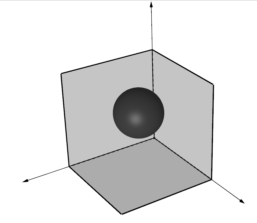
Figure 1. Three square arrays, modelled by $\Gamma_{0}$, in light grey. The dark grey ball depicts the specimen to be imaged.

In order to avoid mathematical technicalities, we will consider wave propagation in an unbounded open and connected set $\Omega\subset\mathbb{R}^{n}$ with smooth boundary. Such $\Omega$ can be seen as an approximation of $\Omega_{0}$. We assume that a strictly positive $c\in C^{\infty}(\overline{\Omega})$ gives the speed of sound in $\Omega$. A PAT measurement on an open set $\Gamma\subset\partial\Omega$ for $T>0$ time units is then modelled by the trace $w|_{(0,T)\times\Gamma}$ where $w$ solves the wave equation

(2) $$\begin{cases}\partial_{t}^{2}w-c^{2}\Delta w=0,&\text{in $(0,T)\times\Omega$},\\ \partial_{\nu}w=0,&\text{in $(0,T)\times\partial\Omega$},\\ w|_{t=0}=w_{0},\ \partial_{t}w|_{t=0}=0,&\text{in $\Omega$},\end{cases}$$

and $\operatorname{supp}(w_{0})\subset\Omega$ is assumed to be compact. The objective is to:

• Recover $w_{0}$ given $w|_{(0,T)\times\Gamma}$.

The finite speed of propagation property satisfied by the solution of (2) implies that if $\operatorname{supp}(w_{0})$ is large in comparison with $\Gamma$ and $T$, then $w|_{(0,T)\times\Gamma}$ does not determine $w_{0}$ uniquely. Indeed, the initial pressure $w_{0}$ is determined by the measurement $w|_{(0,T)\times\Gamma}$ if and only if $d(x,\Gamma)\leq T$ for all $x\in\operatorname{supp}(w_{0})$. Here $d(\cdot,\cdot)$ is the Euclidean distance if $c=1$ identically and $\Omega$ is convex and, in general, it is the distance function on the Riemannian manifold with boundary $(\Omega,c^{-2}dx^{2})$.

In this paper, we introduce a time reversal method that recovers $w_{0}$ given the measurement $w|_{(0,T)\times\Gamma}$, assuming the sharp condition $d(\operatorname{supp}(w_{0}),\Gamma)\leq T$. Moreover, under the further assumption that all the singularities of $w_{0}$ propagate to $\Gamma$ in time $T$, see the condition (VC) below for the precise formulation, we show that the method converges at an exponential rate. To our knowledge, this is the first method with proven exponential convergence rate in the case that measurements are given on a bounded set and the domain of wave propagation is unbounded.

1.1. Previous literature

Our time reversal method is a part of the tradition [9, 17, 24] of back and forth nudging methods originating from [2]. It is also similar to the tradition of time reversal methods [8, 13, 14] and iterative time reversal methods [1, 23, 26, 27, 28].

The closest work to the present one is [22] where a time reversal method similar to ours is introduced in the context of PAT. The method in [22] uses the same stabilizing boundary conditions that we are using, see (5) below, and although the result [22] was obtained independently from the tradition originating from [2], it can be viewed as a part of this tradition in the sense that it fits in the abstract setting [24].

The result [22] assumes the geometric control condition by Bardos, Lebeau and Rauch [3], and this is a global assumption on the whole domain $\Omega$. The main novelty in the present work is that our geometric condition, see (VC) below, is local in the following sense: suppose that the accessible part of the boundary $\Gamma$ is strictly convex (in the sense of the second fundamental form), then our method converges exponentially if $w_{0}$ is supported in a sufficiently small neighbourhood of $\Gamma$. In the case that $c=1$ identically, this neighbourhood is the convex hull of $\Gamma$. Moreover, our result also applies to cases where $\Gamma$ is convex but not strictly convex, an example being (a smooth approximation of) $\Gamma_{0}$ in Figure 1.

We prove the exponential convergence by using microlocal analysis, see Lemma 7 below, and this step can be viewed as a local analogue of [3] under the local condition (VC). Let us also point out that the condition (VC) does not use signals reflected from the inaccessible part of the boundary $\partial\Omega\setminus\Gamma$ and, in particular, it does not require the domain $\Omega$ to be a closed cavity. This is motivated by practical applications since the signal from $w_{0}$ typically deteriorates badly after reflections from $\partial\Omega\setminus\Gamma$. For example, in recent experimental study [6] virtually nothing could be detected after the first two reflections even in media with low acoustic absorption (water in the case of [6]). See also [4, 5] for other experimental studies in case when $\Omega$ is a closed cavity.

Of the above mentioned methods, only [9] is applicable to the case that $\Omega$ is unbounded. The main difference between [9] and the present work is that we show that our method converges to $w_{0}$, whereas in [9] convergence is shown only up to an abstract projection that is not characterised in terms of Sobolev spaces.

Let us also point out that for the iterative time reversal methods that do not use stabilizing boundary conditions [26, 27, 28], exponential convergence has been shown only in the full data case, that is, when the support of $w_{0}$ is enclosed by $\Gamma$. Of these three methods, [28] is the closest to the present one. There the problem (P) is considered in a bounded domain $\Omega$ with Neumann boundary conditions, and the method is shown to converge exponentially when $\Gamma=\partial\Omega$.

2. Statement of the results

Let us formulate our time reversal method in a slightly more general context than (2). Let $(M,g)$ be a smooth Riemannian manifold with boundary, and let $\mu\in C^{\infty}(M)$ be strictly positive. Consider the wave equation,

(3) $$\begin{cases}\partial_{t}^{2}v-\Delta_{g,\mu}v=0,&\text{in $(-T,T)\times M$},\\ \partial_{\nu}v=0,&\text{in $(-T,T)\times\partial M$},\\ v|_{t=0}=v_{0},\ \partial_{t}v|_{t=0}=v_{1},&\text{in $M$},\end{cases}$$

where $\Delta_{g,\mu}$ and $\partial_{\nu}$ are the weighted Laplace-Beltrami operator and the normal derivative,

$$\Delta_{g,\mu}u=\mu^{-1}\operatorname{div}(\mu\nabla u),\quad\partial_{\nu}u=\left\langle\nu,\nabla u\right\rangle.$$

Here $\nu$ is the outward pointing unit normal vector field on $\partial M$, $\operatorname{div}$ and $\nabla$ are the divergence and gradient on $(M,g)$, and $\langle\cdot,\cdot\rangle$ denotes the inner product with respect to the metric $g$. Occasionally, we use also the notation $|\xi|^{2}=\left\langle\xi,\xi\right\rangle$, $\xi\in T_{x}M$, $x\in M$.

Note that the equation (2) is a special case of (3). Indeed, as $\partial_{t}w|_{t=0}=0$, the function

$$v(t,x)=\begin{cases}w(t,x),&t\in(0,T),\\ w(-t,x),&t\in(-T,0),\end{cases}$$

satisfies (3), with $g=c^{-2}dx^{2}$, $\mu=c^{n-2}$, $v_{0}=w_{0}$ and $v_{1}=0$, when $w$ satisfies (2). Let $\Gamma\subset\partial M$ be open and define

$$\Lambda V_{0}=v|_{(-T,T)\times\Gamma},\quad V_{0}=(v_{0},v_{1}),$$

where $v$ is the solution of (3). The PAT problem (P) is a special case of the inverse initial source problem to recover $V_{0}$ given $\Lambda V_{0}$.

We will next introduce the function spaces and operators used in our time reversal iteration. We write for a compact set $\mathcal{K}\subset M$,

$$\mathcal{H}(\mathcal{K})=\{(u_{0},u_{1})\in H^{1}(M)\times L^{2}(M);\ \operatorname{supp}(u_{j})\subset\mathcal{K},\ j=0,1\}.$$

When $\mathcal{K}\neq M$, we equip $\mathcal{H}(\mathcal{K})$ with the energy norm defined by

(4) $$\left\|U\right\|_{*}^{2}=\frac{1}{2}\int_{M}(|\nabla u_{0}|^{2}+|u_{1}|^{2})\,\mu dx,\quad U=(u_{0},u_{1}),$$

where $dx$ stands for the Riemannian volume measure on $(M,g)$. By [21] the map $\Lambda$ is continuous from $\mathcal{H}(\mathcal{K})$ to $H^{1}((-T,T)\times\Gamma)$ when $\mathcal{K}\subset M^{\text{int}}$.

Note that $\left\|\cdot\right\|_{*}$ fails to be norm on $\mathcal{H}(\mathcal{K})$ if $\mathcal{K}=M$, since there are constant non-zero functions $U\in\mathcal{H}(M)$ and $\left\|U\right\|_{*}=0$ for them. To avoid technicalities related to this, we will make the standing assumption that $M$ is unbounded. This assumption reflects also the fact that we are mainly interested in measurement geometries similar to (1).

Let $\Lambda V_{0}$ be a fixed measurement where $V_{0}\in\mathcal{H}(K)$ for a compact set $K\subset M^{\text{int}}$. Define the time intervals $I^{+}=(0,T)$ and $I^{-}=(-T,0)$, and write

$$t_{\uparrow}^{+}=0,\quad t_{\downarrow}^{+}=T,\quad t_{\uparrow}^{-}=-T,\quad t_{\downarrow}^{-}=0,$$

for the boundary points of the intervals $I^{\pm}$. We choose a non-negative cut off function $\chi_{0}\in C_{0}^{\infty}(\partial M)$ satisfying $\operatorname{supp}(\chi_{0})=\overline{\Gamma}$, and consider the wave equation

(5) $$\begin{cases}\partial_{t}^{2}u-\Delta_{g,\mu}u=0,&\text{in $I^{\pm}\times M$},\\ \partial_{\nu}u+\chi\partial_{t}u=\chi\partial_{t}\Lambda V_{0},&\text{in $I^{\pm}\times\partial M$},\\ u|_{t=t_{\uparrow\downarrow}^{\pm}}=u_{0},\ \partial_{t}u|_{t=t_{\uparrow\downarrow}^{\pm}}=u_{1},&\text{in $M$},\end{cases}$$

where $\chi=\chi_{0}$ in the two cases $t_{\uparrow}^{\pm}$ and $\chi=-\chi_{0}$ in the two cases $t_{\downarrow}^{\pm}$. Note that (5) is solved forward in time in the former two cases, and backward in time in the latter two. We write

$$T_{\uparrow}^{+}=T,\quad T_{\downarrow}^{+}=0,\quad T_{\uparrow}^{-}=0,\quad T_{\downarrow}^{-}=-T,$$

for the end point of $I^{\pm}$ opposite to $t_{\uparrow\downarrow}^{\pm}$, and define the nudging operators $N_{\uparrow\downarrow}^{\pm}$ by

$$N_{\uparrow\downarrow}^{\pm}(U_{0};\Lambda V_{0})=(u(T_{\uparrow\downarrow}^{\pm}),\partial_{t}u(T_{\uparrow\downarrow}^{\pm})),$$

where $u$ is the solution of (5) with the initial conditions $U_{0}=(u_{0},u_{1})$ at $t_{\uparrow\downarrow}^{\pm}$.

The iterative step of our time reversal method is given by the average of the two nudging cycles on $I^{+}$ and $I^{-}$ respectively, that is,

$$N(U_{0};\Lambda V_{0}) =\left(N^{+}(U_{0};\Lambda V_{0})+N^{-}(U_{0};\Lambda V_{0})\right)/2,$$

$$N^{+}(U_{0};\Lambda V_{0}) =N_{\downarrow}^{+}(N_{\uparrow}^{+}(U_{0};\Lambda V_{0});\Lambda V_{0}),$$

$$N^{-}(U_{0};\Lambda V_{0}) =N_{\uparrow}^{-}(N_{\downarrow}^{-}(U_{0};\Lambda V_{0});\Lambda V_{0}).$$

We emphasize that the stabilizing boundary condition in (5) is used only in the computational procedure, whereas the measurement data is generated by (3) with homogeneous Neumann boundary condition.

Before stating our results precisely, let us consider informally the iteration $N^{j}$, $j=1,2,\dots$, based on the nudging map $N(U_{0})=N(U_{0};\Lambda V_{0})$. The nudging map $N$ is a contraction (under suitable geometric conditions), since the difference $w$ of two solutions of (5), with different initial conditions, satisfies the stabilizing boundary condition $\partial_{\nu}w+\chi\partial_{t}w=0$, and this causes the energy of $w$ to decrease. Thus $N$ admits a unique fixed point and the iteration $N^{j}U_{0}$ converges to the fixed point for any $U_{0}$. (Below we take $U_{0}=0$ for convenience.) Moreover, the fixed point is $V_{0}$. Indeed, the solution $u$ of (5) with the initial condition $(u_{0},u_{1})=V_{0}$ at the time $t=0$ coincides with the solution $v$ of (3) since

$$\partial_{\nu}v+\chi\partial_{t}v=\chi\partial_{t}v=\chi\partial_{t}\Lambda V_{0}.$$

Hence $N^{+}_{\uparrow}(V_{0};\Lambda V_{0})=(v(T),\partial_{t}v(T))$, and similarly $N^{+}(V_{0};\Lambda V_{0})=(v(0),\partial_{t}v(0))=V_{0}$. The other cycle is analogous, and thus $N(V_{0})=V_{0}$.

Let us now formulate our main results. We define the domain of influence

$$M(\Gamma,T)=\{x\in M;\ d(x,\Gamma)\leq T\},$$

where $d(\cdot,\cdot)$ is the distance function on $(M,g)$, and use the shorthand notation

$$\mathcal{H}=\mathcal{H}(M(\Gamma,T)).$$

Furthermore, we denote by $P_{K}$, $K\subset M(\Gamma,T)$, the orthogonal projection $\mathcal{H}\to\mathcal{H}(K)$ with respect to the energy inner product, that is, the inner product associated to the norm (4).

Due to the finite speed of propagation, it is necessary that $K\subset M(\Gamma,T)$ in order to fully recover $V_{0}\in\mathcal{H}(K)$ given the measurement $\Lambda V_{0}$. Our first result gives a time reversal iteration that converges to $V_{0}$ under this condition.

Theorem 1.

Let $K\subset M^{\text{int}}$ be compact and suppose that $K\subset M(\Gamma,T)$. Then for all $V_{0}\in\mathcal{H}(K)$ it holds that $\lim_{j\to\infty}(P_{K}N)^{j}(0)=V_{0}$ where $N=N(\cdot;\Lambda V_{0})$.

We say that a compact set $K\subset M^{\text{int}}$ satisfies the visibility condition if

• For all $x\in K$ and all $\xi\in T_{x}K$ satisfying $|\xi|=1$ there is $t\in(-T,T)$ such that

  $$\gamma(t;x,\xi)=y\in\Gamma\quad\text{and}\quad\dot{\gamma}(t;x,\xi)\notin T_{y}\Gamma.$$

  Here $\gamma=\gamma(\cdot;x,\xi)$ is the geodesic of $(M,g)$ satisfying $\gamma(0)=x$ and $\dot{\gamma}(0)=\xi$, and we assume that $\gamma$ does not intersect the boundary $\partial M$ between times $0$ and $t$.

Let us point out that a slightly more general version of (VC) is necessary for continuity of the inverse

$$\Lambda^{-1}:H^{1}((-T,T)\times\Gamma)\to\mathcal{H}(K).$$

Indeed, if geodesics $\gamma$ are extended by reflection or suitable gliding when they intersect $\partial M\setminus\Gamma$, see [3] for the precise definition, and if there are $x\in K$ and $\xi\in T_{x}K$ such that $|\xi|=1$ and that the corresponding extended $\gamma$ does not intersect $\Gamma$, then $\Lambda^{-1}$ is not continuous [3, Th. 3.2].

Our second result says that the time reversal iteration converges to $V_{0}$ at an exponential rate, assuming the visibility condition.

Theorem 2.

Let a compact set $K\subset M^{\text{int}}$ satisfy the visibility condition (VC). Then there is a linear map $R:\mathcal{H}(K)\to\mathcal{H}(K)$ such that $\left\|R\right\|_{\mathcal{H}(K)\to\mathcal{H}(K)}<1$ and that for all $V_{0}\in\mathcal{H}(K)$

$$(P_{K}N)^{j}(0)=V_{0}-R^{j}V_{0},\quad j=1,2,\dots,$$

where $N=N(\cdot;\Lambda V_{0})$.

Remark 1.

Under the assumptions of Theorem 2, an alternative reconstruction method is obtained by the Neumann series inversion

$$V_{0}=(1-R)^{-1}P_{K}N(0)=\sum_{j=0}^{\infty}R^{j}P_{K}N(0).$$

Here $R=P_{K}S$, where $S$ is defined in Lemma 2 below.

3. Back and forth nudging identity

We define $S^{\pm}_{\uparrow\downarrow}$ to be the solution operator at time $T_{\uparrow\downarrow}^{\pm}$ of the problem

(6) $$\begin{cases}\partial_{t}^{2}u-\Delta_{g,\mu}u=0,&\text{in $I^{\pm}\times M$},\\ \partial_{\nu}u+\chi\partial_{t}u=0,&\text{in $I^{\pm}\times\partial M$},\\ u|_{t=t_{\uparrow\downarrow}^{\pm}}=u_{0},\ \partial_{t}u|_{t=t_{\uparrow\downarrow}^{\pm}}=u_{1},&\text{in $M$},\end{cases}$$

where $\chi=\chi_{0}$ in the two cases $t_{\uparrow}^{\pm}$ and $\chi=-\chi_{0}$ in the two cases $t_{\downarrow}^{\pm}$. That is,

$$S^{\pm}_{\uparrow\downarrow}U_{0}=(u(T_{\uparrow\downarrow}^{\pm}),\partial_{t}u(T_{\uparrow\downarrow}^{\pm})),$$

where $u$ is the solution of (6) with the initial conditions $U_{0}=(u_{0},u_{1})$ at $t_{\uparrow\downarrow}^{\pm}$.

If $u_{0}\in H^{1}(M)$ and $u_{1}\in L^{2}(M)$ are compactly supported, then the equation (6) has a unique solution $u$ in the energy space $C(I^{\pm};H^{1}(M))\cap C^{1}(I^{\pm};L^{2}(M))$. The sign of $\chi$ is important here, and in fact, the opposite choices of sign do not give well-posed problems. For the convenience of the reader, we have included a study of (6) in the appendix below.

Lemma 1.

Let $V_{0}\in\mathcal{H}(K)$, $W_{0}\in\mathcal{H}$ and define

$$V(t)=(v(t),\partial_{t}v(t)),\quad t\in(-T,T),$$

where $v$ is the solution of (3) with the initial conditions $V_{0}=(v_{0},v_{1})$. Then

$$V(T_{\uparrow\downarrow}^{\pm})+S_{\uparrow\downarrow}^{\pm}(W_{0}-V(t_{\uparrow\downarrow}^{\pm})) =N^{\pm}_{\uparrow\downarrow}(W_{0};\Lambda V_{0}).$$

Proof.

Let $u$ be the solution of (6) with the initial conditions

$$(u|_{t=t_{\uparrow\downarrow}^{\pm}},\partial_{t}u|_{t=t_{\uparrow\downarrow}^{\pm}})=W_{0}-V(t_{\uparrow\downarrow}^{\pm}),$$

and write $W_{0}=(w_{0},w_{1})$. Then the sum $w=u+v$ satisfies

$$\begin{cases}\partial_{t}^{2}w-\Delta_{g,\mu}w=0,&\text{in $I^{\pm}\times M$},\\ \partial_{\nu}w+\chi\partial_{t}w=\chi\partial_{t}v,&\text{in $I^{\pm}\times\partial M$},\\ w|_{t=t_{\uparrow\downarrow}^{\pm}}=w_{0},\ \partial_{t}w|_{t=t_{\uparrow\downarrow}^{\pm}}=w_{1},&\text{in $M$}.\end{cases}$$

We write $W(t)=(w(t),\partial_{t}w(t))$, $t\in(0,T)$, and observe that $W(T_{\uparrow\downarrow}^{\pm})=N_{\uparrow\downarrow}^{\pm}(W_{0};\Lambda V_{0})$ since the above equation for $w$ coincides with the equation (5). The claim follows from

$$W(T_{\uparrow\downarrow}^{\pm})=S_{\uparrow\downarrow}^{\pm}(W_{0}-V(t_{\uparrow\downarrow}^{\pm}))+V(T_{\uparrow\downarrow}^{\pm}).$$

∎

Lemma 2.

Let $V_{0}\in\mathcal{H}(K)$ and $U_{0}\in\mathcal{H}$. Then the following nudging identity holds

(7) $$N(U_{0};\Lambda V_{0})-V_{0}=S(U_{0}-V_{0}),$$

where $S=(S^{+}+S^{-})/2$, $S^{+}=S_{\downarrow}^{+}S_{\uparrow}^{+}$ and $S^{-}=S_{\uparrow}^{-}S_{\downarrow}^{-}$.

Proof.

We omit writing the parameter $\Lambda V_{0}$ in the proof. We apply Lemma 1 twice

$$N_{\downarrow}^{+}(N_{\uparrow}^{+}(U_{0})) =N_{\downarrow}^{+}(V(T)+S_{\uparrow}^{+}(U_{0}-V_{0}))$$

$$=V_{0}+S_{\downarrow}^{+}((V(T)+S_{\uparrow}^{+}(U_{0}-V_{0}))-V(T))$$

$$=V_{0}+S_{\downarrow}^{+}S_{\uparrow}^{+}(U_{0}-V_{0}).$$

An analogous computation for the composition $N^{-}=N_{\uparrow}^{-}N_{\downarrow}^{-}$ shows that

$$N^{-}(U_{0})-V_{0}=S^{-}(U_{0}-V_{0}),$$

and we obtain (7) after taking the average. ∎

4. Energy identity and unique continuation

The following energy identity is well-known, however, we give a short proof for the convenience of the reader.

Lemma 3.

Let a solution $u\in C^{\infty}((0,T)\times M)$ to

$$\begin{cases}\partial_{t}^{2}u-\Delta_{g,\mu}u=0,&\text{in $(0,T)\times M$},\\ \partial_{\nu}u+\chi\partial_{t}u=0,&\text{in $(0,T)\times\partial M$},\end{cases}$$

satisfy $\operatorname{supp}(u)\subset\mathbb{R}\times\mathcal{K}$ where $\mathcal{K}\subset M$ is compact. Then

(8) $$\left\|U(t_{1})\right\|_{*}^{2}=\left\|U(t_{0})\right\|_{*}^{2}-\int_{t_{0}}^{t_{1}}\int_{\partial M}\chi|\partial_{t}u|^{2}\,\mu dydt,\quad t_{0}<t_{1},$$

where $U(t)=(u(t),\partial_{t}u(t))$ and $dy$ is the Riemannian volume measure on $(\partial M,g)$.

Proof.

We first integrate by parts

$$\partial_{t}\left\|U\right\|_{*}^{2} =\int_{M}\partial_{t}^{2}u\,\partial_{t}u+\left\langle\mu\nabla u,\nabla\partial_{t}u\right\rangle\,dx$$

$$=\int_{M}(\partial_{t}^{2}u-\Delta_{g,\mu}u)\,\partial_{t}u\,\mu dx+\int_{\partial M}\partial_{\nu}u\,\partial_{t}u\,\mu dy$$

$$=-\int_{\partial M}\chi|\partial_{t}u|^{2}\,\mu dy,$$

and then integrate in time

$$\left\|U(t_{1})\right\|_{*}^{2}-\left\|U(t_{0})\right\|_{*}^{2}=-\int_{t_{0}}^{t_{1}}\int_{\partial M}\chi|\partial_{t}u|^{2}\,\mu dydt.$$

∎

Lemma 4.

Let a function $u$ in the energy space

(9) $$C((-T,T);H^{1}(M))\cap C^{1}((-T,T);L^{2}(M))$$

satisfy the wave equation

(10) $$\partial_{t}^{2}u-\Delta_{g,\mu}u=0,\quad\text{in $(-T,T)\times M$},$$

and write $U_{0}=(u|_{t=0},\partial_{t}u|_{t=0})$. Let $K\subset M^{\text{int}}\cap M(\Gamma,T)$ be compact. Suppose, furthermore, that $U_{0}\in\mathcal{H}(K)$, $\partial_{\nu}u=0$ on $(-T,T)\times\partial M$ and that $\partial_{t}u=0$ on $(-T,T)\times\Gamma$. Then $U_{0}=0$.

Proof.

We write $U_{0}=(u_{0},u_{1})$. Suppose for the moment that $u\in C^{\infty}((-T,T)\times M)$. The function $w=\partial_{t}u$ satisfies (10) and both $w$ and $\partial_{\nu}w$ vanish on $(-T,T)\times\Gamma$. The semi-global version [18, Th. 3.16] of the time sharp unique continuation result [29], implies that $w$ vanishes in the double cone of points $(t,x)$ satisfying $d(x,\Gamma)\leq T-|t|$. In particular, $w|_{t=0}=u_{1}=0$ in $M(\Gamma,T)$. The assumption $U_{0}\in\mathcal{H}(K)$ implies that $u_{1}=0$ also outside $M(\Gamma,T)$. Furthermore, as $w$ vanishes in the double cone, also $\partial_{t}w=\Delta_{g,\mu}u$ vanishes there. Thus $\Delta_{g,\mu}u_{0}=0$ in $M(\Gamma,T)$. The assumption $U_{0}\in\mathcal{H}(K)$ together with $K\subset M^{\text{int}}$ implies that $u_{0}$ vanishes near $\Gamma$, and therefore $u_{0}=0$ in $M(\Gamma,T)$ by elliptic unique continuation. Finally, $u_{0}=0$ outside $M(\Gamma,T)$ by the assumption $U_{0}\in\mathcal{H}(K)$.

Let us now consider the general case where $u$ is in (9). Let $\psi\in C_{0}^{\infty}(-\epsilon/2,\epsilon/2)$, where $\epsilon>0$ is small. We extend $u$ by zero to a function on $\mathbb{R}\times M$ and denote the extension still by $u$. The convolution in time $w=\psi*\partial_{t}u$ satisfies (10) on $(-T+\epsilon,T-\epsilon)\times M$, and the Cauchy data $(w,\partial_{\nu}w)$ vanishes on $(-T+\epsilon,T-\epsilon)\times\Gamma$. Note that $w\in C^{\infty}(\mathbb{R};L^{2}(M))$. Let $t\in\mathbb{R}$ satisfy $|t|<T-\epsilon$. Then

(11) $$\Delta_{g,\mu}w(t)=\partial_{t}^{2}w(t)\in L^{2}(M).$$

As the spatial support of $u$ is contained in the compact set $\mathcal{K}$, there is a compact manifold with smooth boundary $M_{0}\subset M$ such that $M(\Gamma,T)\subset M_{0}$ and $\partial_{\nu}w(t)=0$ on $\partial M_{0}$. As $w(t)$ satisfies (11) with vanishing Neumann boundary conditions on $M_{0}$, it holds that $w(t)\in H^{2}(M_{0})$, see e.g. [30, Prop. 7.6]. Hence we may apply [18, Th. 3.16] on $w$. As above, we see that both $\psi*u_{1}$ and $\Delta_{g,\mu}(\psi*u_{0})$ vanish on $M(\Gamma,T-\epsilon)$. Letting $\phi\to\delta$ and $\epsilon\to 0$, we get

$$u_{1}=\Delta_{g,\mu}u_{0}=0\quad\text{on $M(\Gamma,T)^{\text{int}}$}.$$

Using the assumption $U_{0}\in\mathcal{H}(K)$ as above, we see that $U_{0}=0$. ∎

Lemma 5.

Let $K\subset M^{\text{int}}\cap M(\Gamma,T)$ be compact. Let $U_{0}\in\mathcal{H}(K)$, and consider the function

$$u(t,x)=\begin{cases}u^{+}(t,x),&t\geq 0,\\ u^{-}(t,x),&t\leq 0,\end{cases}$$

where $u^{\pm}$ are the solutions of (6) with the initial conditions given by $U_{0}$ at $t_{\uparrow}^{+}$ and $t_{\downarrow}^{-}$ respectively. Then

$$\left\|SU_{0}\right\|_{*}^{2}\leq\left\|U_{0}\right\|_{*}^{2}-\frac{1}{2}\int_{-T}^{T}\int_{\partial M}\chi_{0}|\partial_{t}u|^{2}\,\mu dydt.$$

Moreover, the continuous map

$$E:\mathcal{H}(K)\to L^{2}((-T,T)\times\partial M),\quad EU_{0}=\sqrt{\chi_{0}}\partial_{t}u,$$

is injective.

Proof.

Suppose for the moment that $U_{0}\in C_{0}^{\infty}(K)^{2}$. Then both $u^{\pm}$ are smooth, see Theorem 3 in the appendix below. As $\chi_{0}$ is non-negative, the energy identity (8) implies that

$$\left\|S_{\uparrow\downarrow}^{\pm}U_{0}\right\|_{*}\leq\left\|U_{0}\right\|_{*}.$$

Note that for the backward propagators $S_{\downarrow}^{\pm}$ we use the fact that $\chi=-\chi_{0}$. It holds that

$$\left\|SU_{0}\right\|_{*}^{2} \leq\frac{1}{4}\left(\left\|S_{\downarrow}^{+}S_{\uparrow}^{+}U_{0}\right\|_{*}+\left\|S_{\uparrow}^{-}S_{\downarrow}^{-}U_{0}\right\|_{*}\right)^{2}\leq\frac{1}{2}\left(\left\|S_{\uparrow}^{+}U_{0}\right\|_{*}^{2}+\left\|S_{\downarrow}^{-}U_{0}\right\|_{*}^{2}\right)$$

$$=\frac{1}{2}\left(\left\|U_{0}\right\|_{*}^{2}-\int_{0}^{T}\int_{\partial M}\chi_{0}|\partial_{t}u|^{2}\,\mu dydt+\left\|U_{0}\right\|_{*}^{2}-\int_{-T}^{0}\int_{\partial M}\chi_{0}|\partial_{t}u|^{2}\,\mu dydt\right)$$

$$=\left\|U_{0}\right\|_{*}^{2}-\frac{1}{2}\int_{-T}^{T}\int_{\partial M}\chi_{0}|\partial_{t}u|^{2}\,\mu dydt.$$

The general case $U_{0}\in\mathcal{H}(K)$ follows since $C_{0}^{\infty}(K)^{2}$ is dense in $\mathcal{H}(K)$.

Suppose now that $EU_{0}=0$. Then $\partial_{\nu}u=0$ on $(-T,T)\times\partial M$ and, using the assumption $\operatorname{supp}(\chi_{0})=\overline{\Gamma}$, we see that $\partial_{t}u=0$ on $(-T,T)\times\Gamma$. Note that by Theorem 3 (cf. Appendix) $u^{+}$ is in the energy space (19) and $u^{-}$ is in the corresponding energy space on $[-T,0]$. As $K\subset M^{int}$, we see that $u$ belongs to the space (9). Lemma 4 implies that $U_{0}=0$. ∎

5. The unstable case

Lemma 6.

The operator $P_{K}S:\mathcal{H}(K)\to\mathcal{H}(K)$ is self-adjoint and positive.

Proof.

Let us show that $P_{K}S^{+}$ is self-adjoint and positive. The case $P_{K}S^{-}$ is similar and we omit it. We write $U_{\uparrow\downarrow}(t)=(u_{\uparrow\downarrow}(t),\partial_{t}u_{\uparrow\downarrow}(t))$ where $u_{\uparrow}$ and $u_{\downarrow}$ are smooth solutions of

(12) $$\begin{cases}\partial_{t}^{2}u-\Delta_{g,\mu}u=0,&\text{in $(0,T)\times M$},\\ \partial_{\nu}u+\chi\partial_{t}u=0,&\text{in $(0,T)\times\partial M$},\end{cases}$$

with $\chi=\chi_{0}$ and $\chi=-\chi_{0}$, respectively. Then, writing $\left\langle\cdot,\cdot\right\rangle_{M}$ and $\left\langle\cdot,\cdot\right\rangle_{\partial M}$ for the $L^{2}$ inner products on $M$ and $\partial M$ with respect to the measures used in Lemma 3,

$$\partial_{t}\left\langle U_{\uparrow},U_{\downarrow}\right\rangle_{*} =\left\langle\partial_{t}^{2}u_{\uparrow},\partial_{t}u_{\downarrow}\right\rangle_{M}+\left\langle\nabla u_{\uparrow},\nabla\partial_{t}u_{\downarrow}\right\rangle_{M}+\left\langle\partial_{t}u_{\uparrow},\partial_{t}^{2}u_{\downarrow}\right\rangle_{M}+\left\langle\nabla\partial_{t}u_{\uparrow},\nabla u_{\downarrow}\right\rangle_{M}$$

$$=\left\langle\chi_{0}\partial_{t}u_{\uparrow},\partial_{t}u_{\downarrow}\right\rangle_{\partial M}-\left\langle\partial_{t}u_{\uparrow},\chi_{0}\partial_{t}u_{\downarrow}\right\rangle_{\partial M}=0.$$

Hence $\left\langle U_{\uparrow}(0),U_{\downarrow}(0)\right\rangle_{*}=\left\langle U_{\uparrow}(T),U_{\downarrow}(T)\right\rangle_{*}$.

Let $U_{0}\in C_{0}^{\infty}(K)^{2}$, and let $U_{\uparrow}(t)=(u_{\uparrow},\partial_{t}u_{\uparrow}(t))$ where $u_{\uparrow}$ satisfies (12) with $\chi=\chi_{0}$ and also the initial condition $U_{\uparrow}(0)=U_{0}$. Then $U_{\uparrow}$ is smooth, see Theorem 3 in the appendix below. Set $U^{r}_{\downarrow}(t)=(u(t),\partial_{t}u(t))$ where $u(t)=u_{\uparrow}(2T-t)$. Then $u$ satisfies (12) with $\chi=-\chi_{0}$, and also $U^{r}_{\downarrow}(T)=(u_{\uparrow}(T),-\partial_{t}u_{\uparrow}(T))$. Let $\phi_{j}\in C_{0}^{\infty}(M)$ converge to $2\partial_{t}u_{\uparrow}(T)$ in $L^{2}(M)$, and write $U_{\downarrow}^{j}(t)=(u_{\downarrow}^{j}(t),\partial_{t}u_{\downarrow}^{j}(t))$ where $u^{j}$ is the solution of (12) with $\chi=-\chi_{0}$ satisfying $U_{\downarrow}^{j}(T)=(0,\phi_{j})$. Denote by $U_{\downarrow}$ the solution of (12) with $\chi=-\chi_{0}$ satisfying $U_{\downarrow}(T)=U_{\uparrow}(T)=S^{+}_{\uparrow}U_{0}$.

Let $W_{0}\in C_{0}^{\infty}(K)^{2}$. As $U^{r}_{\downarrow}$ and $U_{\downarrow}^{j}$, $j\in\mathbb{N}$, are smooth, we have

$$\left\langle W_{0},S^{+}_{\downarrow}S^{+}_{\uparrow}U_{0}\right\rangle_{*} =\left\langle W_{0},U_{\downarrow}(0)\right\rangle_{*}=\lim_{j\to\infty}\left\langle W_{0},U^{r}_{\downarrow}(0)+U_{\downarrow}^{j}(0)\right\rangle_{*}$$

$$=\lim_{j\to\infty}\left\langle S^{+}_{\uparrow}W_{0},U^{r}_{\downarrow}(T)+U_{\downarrow}^{j}(T)\right\rangle_{*}=\left\langle S^{+}_{\uparrow}W_{0},S^{+}_{\uparrow}U_{0}\right\rangle_{*}.$$

The above computation, with the roles of $W_{0}$ and $U_{0}$ interchanged, implies that

$$\left\langle S^{+}_{\downarrow}S^{+}_{\uparrow}W_{0},U_{0}\right\rangle_{*}=\left\langle S^{+}_{\uparrow}W_{0},S^{+}_{\uparrow}U_{0}\right\rangle_{*}=\left\langle W_{0},S^{+}_{\downarrow}S^{+}_{\uparrow}U_{0}\right\rangle_{*}.$$

The same holds for all $U_{0},W_{0}\in\mathcal{H}(K)$ by density, which again shows that $P_{K}S^{+}$ is self-adjoint and positive. ∎

The following proof is an adaptation of the proof of [9, Th. 1.1]. The main difference is that the result in [9] is given in an abstract setting that does not allow for a full characterization of the convergence.

Proof of Theorem 1.

By Lemma 2,

$$P_{K}N(U_{0})-V_{0}=P_{K}(N(U_{0})-V_{0})=P_{K}S(U_{0}-V_{0}),\quad U_{0}\in\mathcal{H}.$$

We iterate this starting from $U_{0}=0$. That is, for $j=1,2,\dots$,

(13) $$(P_{K}N)^{j}(0)-V_{0}=P_{K}S((P_{K}N)^{j-1}(0)-V_{0})=-(P_{K}S)^{j}V_{0}.$$

Writing $R=P_{K}S$, it remains to show that the sequence $R^{j}V_{0}$, $j\in\mathbb{N}$, converges to zero.

By Lemma 6, the operator $R$ is self-adjoint and positive, and whence also the powers $R^{j}$, $j\in\mathbb{N}$, are self-adjoint and positive. We will use the fact that a non-increasing sequence of bounded positive operators in a Hilbert space converges pointwise to a bounded operator, see e.g. [31, Lem. 12.3.2].

Lemma 5 implies that $\left\|SV_{0}\right\|_{*}\leq\left\|V_{0}\right\|_{*}$, $V_{0}\in\mathcal{H}(K)$, and that the equality holds only if $V_{0}=0$. Hence

$$\left\|R(R^{j/2}V_{0})\right\|_{*}=\left\|P_{K}S(R^{j/2}V_{0})\right\|_{*}\leq\left\|R^{j/2}V_{0}\right\|_{*},\quad j\in\mathbb{N},\ V_{0}\in\mathcal{H}(K),$$

which again implies that the sequence $R^{j}$, $j\in\mathbb{N}$, is non-increasing. Indeed,

$$\langle R^{j+1}V_{0},V_{0}\rangle_{*} =\langle R(R^{j/2}V_{0}),R^{j/2}V_{0}\rangle_{*}\leq\|R(R^{j/2}V_{0})\|_{*}\|R^{j/2}V_{0}\|_{*}$$

$$\leq\|R^{j/2}V_{0}\|_{*}^{2}=\langle R^{j/2}V_{0},R^{j/2}V_{0}\rangle_{*}=\langle R^{j}V_{0},V_{0}\rangle_{*},\quad V_{0}\in\mathcal{H}(K).$$

Therefore the sequence $R^{j}$, $j\in\mathbb{N}$, converges pointwise on $\mathcal{H}(K)$, say to an operator $R^{\infty}$, and it remains to prove that $R^{\infty}=0$.

Observe that $RR^{\infty}=R^{\infty}$, since for all $V_{1},V_{2}\in\mathcal{H}(K)$

$$\langle RR^{\infty}V_{1},V_{2}\rangle_{*}=\lim_{j\to\infty}\langle RR^{j}V_{1},V_{2}\rangle_{*}=\lim_{j\rightarrow\infty}\langle R^{j+1}V_{1},V_{2}\rangle_{*}=\langle R^{\infty}V_{1},V_{2}\rangle_{*}.$$

To get a contradiction, we assume that there is $V_{0}\in\mathcal{H}(K)$ such that $R^{\infty}V_{0}\neq 0$. Then Lemma 5 implies

$$\|R^{\infty}V_{0}\|^{2}_{*}=\langle RR^{\infty}V_{0},R^{\infty}V_{0}\rangle_{*}\leq\left\|P_{K}SR^{\infty}V_{0}\right\|_{*}\left\|R^{\infty}V_{0}\right\|_{*}<\left\|R^{\infty}V_{0}\right\|_{*}^{2},$$

which is indeed a contradiction. ∎

6. The stable case

In this section we prove Theorem 2 using techniques that are similar to those in [3]. The main difference between Lemma 7 below and [3, Th. 3.3] is that we give a local result under the local geometric assumption (VC), whereas [3] gives a global result under a global geometric assumption.

We will use the notion of microlocal regularity at a point, see e.g. [11, Def. 18.1.30]. Recall that a distribution $u$ on $M$ is said to be microlocally $H^{s}$ at $(x,\xi)\in T^{*}M\setminus 0$ if $u=u_{0}+u_{1}$ where $(x,\xi)\notin\operatorname{WF}(u_{0})$ and $u_{1}\in H^{s}_{loc}(M)$. In this case we write $u\in H^{s}(x,\xi)$. Here $\operatorname{WF}$ denotes the wave front set, see [12, Def. 8.1.2], and $H^{s}_{loc}(M)$, $s\in\mathbb{R}$, is the space of distributions $w$ such that $\phi w$ is in the Sobolev space $H^{s}(M)$ for all $\phi\in C_{0}^{\infty}(M)$.

If $u\in H^{s}(x,\xi)$ then by [12, Th. 18.1.31] there is a pseudodifferential operator of order zero $A$ such that $Au\in H^{s}_{loc}(M)$ and $(x,\xi)$ is not characteristic for $A$. Moreover, by [12, Th. 18.1.24’] there is a pseudodifferential operator of order zero $B$ such that

(14) $$(x,\xi)\notin\operatorname{WF}(1-BA)$$

where $1$ is the identity map. Note also that after multiplication by a function $\phi\in C_{0}^{\infty}(M)$ satisfying $\phi=1$ near $x$, we may assume that $Au\in H^{s}(M)$.

Figure 2. The localization and microlocalization. Here the large grey ellipse indicates the set on which $\psi=1$, and the small grey ellipse indicates the base space projection of the set on which (14) holds.

Lemma 7.

Suppose that the condition (VC) holds for a compact set $K\subset M^{\text{int}}$. Let $u\in L^{2}((-T,T)\times M)$ satisfy the wave equation

$$\partial_{t}^{2}u-\Delta_{g,\mu}u=0~{}~{}\mathrm{in}~{}(-T,T)\times M,$$

and suppose that $\partial_{t}u|_{x\in\Gamma},\partial_{\nu}u|_{x\in\Gamma}\in L_{loc}^{2}((-T,T)\times\Gamma)$. Then $u|_{\{t=0\}\times K}\in H^{1}(K)$ and $\partial_{t}u|_{\{t=0\}\times K}\in L^{2}(K)$.

Proof.

By compactness of $K$ there is a neighbourhood $\tilde{K}\subset M^{\text{int}}$ of $K$ and $\epsilon>0$ such that (VC) holds with $K$ replaced by $\tilde{K}$ and $T$ replaced by $T-\epsilon$. Finite speed of propagation and the associated energy estimate imply that it is enough to show that $u\in H^{1}((-\epsilon,\epsilon)\times\tilde{K})$. By using a microlocal partition of unity, it is enough to show that $u\in H^{1}(p_{0})$ at each point $p_{0}\in T^{*}((-\epsilon,\epsilon)\times\tilde{K})$, see [11, Th. 18.1.31]. Furthermore, it is enough to consider characteristic points for the wave operator, that is, points in the set $\{(t,x,\tau,\xi)\in T^{*}(\mathbb{R}\times M^{\text{int}})\setminus 0;\ \tau^{2}=|\xi|^{2}\},$ since $\operatorname{WF}(u)$ is contained in this set.

We assume now that $p_{0}\in T^{*}((-\epsilon,\epsilon)\times\tilde{K})$ is a characteristic point and let $\gamma$ be the bicharacteristic passing through $p_{0}$. The visibility condition (VC) says that $\gamma$ intersects the boundary $\partial T^{*}(\mathbb{R}\times M)$ non-tangentially at a point $q$ that lies over the set $(-T,T)\times\Gamma$. We write $q=(t_{0},y_{0},0;\tau_{0},\eta_{0},\sigma_{0})$ in such local coordinates $(y,s)$ of $M$ that $s=0$ describes the boundary $\partial M$. Then (VC) means that $y_{0}\in\Gamma$ and $\sigma_{0}\neq 0$. We may assume without loss of generality that $t_{0}\in(0,T)$, the case $t_{0}\in(-T,0)$ being analogous.

We denote by $q^{T}=(t_{0},y_{0};\tau_{0},\eta_{0})$ the projection of $q$ on $T^{*}(\mathbb{R}\times\partial M)$, and consider the time derivative $\partial_{t}$ as an operator on the boundary $\mathbb{R}\times\partial M$. As $\tau_{0}\neq 0$, we see that $q^{T}$ is not characteristic for $\partial_{t}$. Together with the assumption $\partial_{t}u\in L_{loc}^{2}((-T,T)\times\Gamma)$ this implies that $u\in H^{1}(q^{T})$, see [11, Th. 18.1.31].

Since $\sigma_{0}\neq 0$, we have that $\tau_{0}^{2}\neq|\eta_{0}|_{g}^{2}$, and therefore $q^{T}$ is not characteristic for the wave operator. By [3, Th. 2.1] there is a tangential pseudodifferential operator $A=A(t,y,D_{t},D_{y})$ of order zero and a neighbourhood $\mathcal{U}\subset\mathbb{R}\times M^{\text{int}}$ of $(t_{0},y_{0},0)$ such that $q^{T}$ is not characteristic for $A$ and $Au\in H^{1}(\mathcal{U})$. The set of characteristic points is closed and this, together with the fact that $A$ is tangential, implies that there is $p_{1}\in\gamma\cap T^{*}(\mathbb{R}\times M^{\text{int}})$ such that $p_{1}$ is not characteristic for $A$. After multiplication by a cut-off function, we may assume that $Au\in H^{1}(\mathbb{R}\times M)$.

For two distinct points $p,\tilde{p}\in\gamma$, we denote the segment of $\gamma$ between $p$ and $\tilde{p}$ by $\sigma(p,\tilde{p})$. As discussed above, there is a pseudodifferential operator of order zero $B$ such that (14) holds with $(x,\xi)$ replaced by $p_{1}$. As the wave front set is closed, there is a point $p_{2}\in\sigma(p_{1},q)$, distinct from $p_{1}$ and $q$, such that (14) holds with $(x,\xi)$ replaced by any point in the segment $\sigma(p_{1},p_{2})$. We denote by $T_{0}$ the time coordinate of $p_{2}$, and choose $\psi\in C_{0}^{\infty}((-T,T_{0})\times M^{\text{int}})$ satisfying $\psi=1$ in a neighbourhood of $\sigma(p_{0},p_{1})$, see Figure 2.

We define $\Phi=[\Box,\psi]u$ where $[\Box,\psi]$ is the commutator of $\Box=\partial_{t}^{2}-\Delta_{g,\mu}$ and $\psi$. Then $\psi u$ satisfies the equation

(15) $$\begin{cases}\Box u=F,&\mathrm{in}~{}(-T,T_{0})\times M,\\ u=0,&\mathrm{in}~{}(-T,T_{0})\times\partial M,\\ u|_{t=T_{0}}=\partial_{t}u|_{t=T_{0}}=0,&\mathrm{in}~{}M,\\ \end{cases}$$

with $F=\Phi$. We consider also the solutions $u_{0}$ and $u_{1}$ of (15) with $F=(1-BA)\Phi$ and $F=BA\Phi$, respectively. Clearly, $\psi u=u_{0}+u_{1}$ and we will establish $u\in H^{1}(p_{0})$ by showing that that $p_{0}\notin\operatorname{WF}(u_{0})$ and $u_{1}\in H^{1}((-T,T_{0})\times M)$.

Let us consider first $u_{0}$. We have $\sigma(p_{0},p_{2})\subset T^{*}(\mathbb{R}\times M^{\text{int}})$ and $u_{0}=0$ for $T_{0}>0$. In view of propagation singularities in the interior [11, Th. 23.2.9], it is enough to show that

$$\operatorname{WF}((1-BA)\Phi)\cap\sigma(p_{0},p_{2})=\emptyset.$$

Now (14) implies that $\operatorname{WF}((1-BA)\Phi)\cap\sigma(p_{1},p_{2})=\emptyset$. Moreover, $\Phi=0$ near $\sigma(p_{0},p_{1})$ since $\psi=1$ there, which again implies that $\operatorname{WF}((1-BA)\Phi)\cap\sigma(p_{0},p_{1})=\emptyset$.

We turn to $u_{1}$. We have

$$A\Phi=[\Box,\psi]Au+[A,[\Box,\psi]]u\in L^{2}((-T,T_{0})\times M),$$

since $Au\in H^{1}((-T,T_{0})\times M)$, $u\in L^{2}((-T,T_{0})\times M)$, and the commutators $[\Box,\psi]$ and $[A,[\Box,\psi]]$ are of order one and zero, respectively. As $B$ is of order zero, we have

$$BA\Phi\in L^{2}((-T,T_{0})\times M),$$

and the energy estimate for (15) implies that $u_{1}\in H^{1}((-T,T_{0})\times M)$. ∎

Theorem 2 follows from (13) and the below lemma.

Lemma 8.

Suppose that the condition (VC) holds for a compact set $K\subset M^{\text{int}}$. Then $\left\|S\right\|_{\mathcal{H}(K)\to\mathcal{H}}<1$.

Proof.

We define two spaces as follows

$$X =\{u\in L^{2}((-T,T)\times M);\ \Box u=0,\ \sqrt{\chi_{0}}\partial_{t}u,\partial_{\nu}u\in L^{2}((-T,T)\times\Gamma)\},$$

$$Y =\{u\in L^{2}((-T,T)\times M);\ \Box u=0,\ u|_{\{t=0\}\times K}\in H^{1}(K),\ \partial_{t}u|_{\{t=0\}\times K}\in L^{2}(K)\}.$$

They are Banach spaces with respect to norms,

$$\|u\|_{X} =\|u\|_{L^{2}((-T,T)\times M)}+\|\sqrt{\chi_{0}}\partial_{t}u\|_{L^{2}((-T,T)\times\Gamma)}+\|\partial_{\nu}u\|_{L^{2}((-T,T)\times\Gamma)},$$

$$\|u\|_{Y} =\|u\|_{L^{2}((-T,T)\times M)}+\|u|_{\{t=0\}\times K}\|_{H^{1}(K)}+\|\partial_{t}u|_{\{t=0\}\times K}\|_{L^{2}(K)},$$

and Lemma 7 implies that $X\subset Y$. The identity map is closed from $X$ to $Y$ since both the norms are stronger than that of $L^{2}((-T,T))\times M)$. The closed graph theorem implies that there is $C>0$ such that $\|u\|_{Y}\leq C\|u\|_{X}$ for all $u\in X$.

Let $U_{0}\in\mathcal{H}(K)$ and consider the function $u$ defined in Lemma 5. Then $\sqrt{\chi_{0}}\partial_{t}u$ is in $L^{2}((-T,T)\in\partial M)$. The boundary condition in (6) implies that $u\in X$ and, together with $U_{0}\in\mathcal{H}(K)$, it implies that the estimate $\|u\|_{Y}\leq C\|u\|_{X}$ reduces to

(16) $$\left\|U_{0}\right\|_{*}\leq C\left(\|\sqrt{\chi_{0}}\partial_{t}u\|_{L^{2}((-T,T)\times\Gamma)}+\left\|u\right\|_{L^{2}(-T,T)\times M)}\right).$$

As $\operatorname{supp}(U_{0})\subset K$, we can choose a compact set $M_{0}\subset M$ such that $u$ is supported in $[-T,T]\times M_{0}$. The embedding $H^{1}((-T,T)\times M_{0})\subset L^{2}((-T,T)\times M_{0})$ is compact, and whence the map $U_{0}\mapsto u$ is compact from $\mathcal{H}(K)$ to $L^{2}((-T,T)\times M_{0})$. By Lemma 5, the map $U_{0}\mapsto\sqrt{\chi_{0}}\partial_{t}u|_{(-T,T)\times\Gamma}$ is injective. Thus the estimate (16) improves to

(17) $$\left\|U_{0}\right\|_{*}\leq C\left\|\sqrt{\chi_{0}}\partial_{t}u\right\|_{L^{2}((-T,T)\times\Gamma)},$$

by using the compactness-uniqueness argument. For the convenience of the reader, we have included the proof of this argument, see Lemma 9 below. The claimed norm estimate follows now from Lemma 5. ∎

Lemma 9 (Compactness-uniqueness).

Let $X$, $Y$ and $Z$ be Banach spaces and let $A:X\to Y$ and $K:X\to Z$ be continuous linear maps. Suppose that $A$ is injective, $K$ is compact and that there is $C>0$ such that

$$\left\|x\right\|_{X}\leq C\left\|Ax\right\|_{Y}+C\left\|Kx\right\|_{Z},\quad x\in X.$$

Then there is $C>0$ such that $\left\|x\right\|_{X}\leq C\left\|Ax\right\|_{Y}$ for $x\in X.$

Proof.

To get a contradiction suppose that there is a sequence $x_{j}\in X$, $j\in\mathbb{N}$, such that $\left\|x_{j}\right\|_{X}=1$ for all $j$ and that $\left\|Ax_{j}\right\|_{Y}\to 0$ as $j\to\infty$. By compactness of $K$, there is a subsequence, still denoted by $x_{j}$, $j\in\mathbb{N}$, such that $Kx_{j}$, $j\in\mathbb{N}$, is a Cauchy sequence. Hence

$$C^{-1}\left\|x_{j}-x_{k}\right\|_{X} \leq\left\|A(x_{j}-x_{k})\right\|_{Y}+\left\|K(x_{j}-x_{k})\right\|_{Z}$$

$$\leq\left\|Ax_{j}\right\|_{Y}+\left\|Ax_{k}\right\|_{Y}+\left\|Kx_{j}-Kx_{k}\right\|_{Z}\to 0,\quad j,k\to\infty.$$

Thus $x_{j}$, $j\in\mathbb{N}$, is a Cauchy sequence, and therefore it converges, say to $x$. We have

$$\left\|x\right\|_{X}=\lim_{j\to\infty}\left\|x_{j}\right\|_{X}=1,\quad\left\|Ax\right\|_{Y}=\lim_{j\to\infty}\left\|Ax_{j}\right\|_{Y}=0,$$

which is a contradiction to the injectivity of $A$. ∎

Appendix. Wave equation with stabilizing boundary conditions

In this appendix we consider the problem (6). For simplicity, we consider only the case $\mu=1$ and write $\Delta=\Delta_{g,\mu}$. The modifications required in the case of a non-constant $\mu$ are straightforward. The following theorem is well-known. For the convenience of the reader we give here a short proof with a reduction to the results in [16].

Theorem 3.

Let $\chi\in C^{\infty}(\partial M)$ be non-negative. Then the equation

(18) $$\begin{cases}\partial_{t}^{2}u-\Delta u=0,&\text{in $(0,T)\times M$},\\ \partial_{\nu}u+\chi\partial_{t}u=0,&\text{in $(0,T)\times\partial M$},\\ u|_{t=0}=u_{0},\ \partial_{t}u|_{t=0}=u_{1},&\text{in $M$},\end{cases}$$

has a unique solution $u$ in the space

(19) $$\mathcal{E}=C([0,T];H^{1}(M))\cap C^{1}([0,T];L^{2}(M))$$

for any $u_{0}\in H^{1}(M)$ and $u_{1}\in L^{2}(M)$ with compact $\operatorname{supp}(u_{j})\subset M$, $j=0,1$. Moreover, if $u_{0},u_{1}\in C_{0}^{\infty}(K)$ and $K\subset M^{\text{int}}$ is compact, then the solution $u$ is smooth.

Proof.

If $u_{0},u_{1}\in C_{0}^{\infty}(K)$ then the claim immediately follows from [16]. Choose $u_{0}\in H^{2}(M)$ such that $\partial_{\nu}u_{0}=0$ on $\partial M$, and $u_{1}\in H_{0}^{1}(M)$. Then [16] implies that (18) has unique solution $u\in H^{2}((0,T)\times M)$.

We define the energy as

$$E(t)=\int_{M}|u(t)|^{2}+|\partial_{t}u(t)|^{2}+|\nabla u(t)|^{2}\,\mu dx,$$

and, analogously to the proof of Lemma 3, we have

$$\partial_{t}E\leq CE+\left\|\partial_{t}^{2}u-\Delta u\right\|_{L^{2}(M)}^{2}.$$

Grönwall’s inequality implies that

(20) $$E(t)\leq CE(0)+C\left\|\partial_{t}^{2}u-\Delta u\right\|_{L^{2}((0,T)\times M)}^{2},\quad t\in(0,T).$$

Thus,

$$\left\|u\right\|_{\mathcal{E}}\leq C\left\|u_{0}\right\|_{H^{1}(M)}+C\left\|u_{1}\right\|_{L^{2}(M)}.$$

Lemma 10 below implies that the map $(u_{0},u_{1})\mapsto u$ has a unique continuous extension

$$H^{1}(M)\times L^{2}(M)\to\mathcal{E},$$

which concludes the proof of the theorem. ∎

Lemma 10.

Let $u\in H^{1}(M)$. Then there is a sequence $u_{j}\in H^{2}(M)$, $j\in\mathbb{N}$, such that $u_{j}\to u$ in $H^{1}(M)$ and $\partial_{\nu}u_{j}=0$ on $\partial M$ for all $j\in\mathbb{N}$.

Proof.

Consider a right inverse of the trace map

$$P:H^{3/2}(\partial M)\times H^{1/2}(\partial M)\to H^{2}(M),\quad\partial_{\nu}^{k}P(h_{0},h_{1})|_{\partial M}=h_{k},\quad k=0,1.$$

Let a sequence $\phi_{j}\in C^{\infty}(M)$, $j\in\mathbb{N}$, converge to $u$ in $H^{1}(M)$. Write $w_{j}=P(\phi_{j},0)$ and $\tilde{u}_{j}=\phi_{j}-w_{j}$. Then $\tilde{u}_{j}\in H_{0}^{1}(M)$ and there is $\psi_{j}\in C_{0}^{\infty}(M)$ such that $\left\|\psi_{j}-\tilde{u}_{j}\right\|_{H^{1}(M)}\leq 1/j$. Set $u_{j}=\psi_{j}+w_{j}$. Then $u_{j}\in H^{2}(M)$, $\partial_{\nu}u_{j}=\partial_{\nu}w_{j}=0$ on $\partial M$ and

$$\left\|u_{j}-u\right\|_{H^{1}(M)}\leq\left\|\psi_{j}-\tilde{u}_{j}\right\|_{H^{1}(M)}+\left\|\tilde{u}_{j}+w_{j}-u\right\|_{H^{1}(M)}\leq 1/j+\left\|\phi_{j}-u\right\|_{H^{1}(M)}\to 0.$$

∎

Acknowledgements. The research was supported by EPSRC grant EP/L026473/1. The authors thank C. Laurent for introducing them to [17], and G. Haine and B. Cox for useful discussions. Moreover, the authors thank P. Stefanov for bringing [22] to their attention. The authors are grateful to the anonymous referees for their comments, which helped to improve the paper.

References

- [1] S. Acosta and C. Montalto. Multiwave imaging in an enclosure with variable wave speed. Inverse Problems, 31(6):065009, 12, 2015.
- [2] D. Auroux and J. Blum. Back and forth nudging algorithm for data assimilation problems. C. R. Math. Acad. Sci. Paris, 340(12):873–878, 2005.
- [3] C. Bardos, G. Lebeau, and J. Rauch. Sharp sufficient conditions for the observation, control, and stabilization of waves from the boundary. SIAM J. Control Optim., 30(5):1024–1065, 1992.
- [4] B. Cox, S. Arridge, and P. Beard. Photoacoustic tomography with a limited-aperture planar sensor and a reverberant cavity. Inverse Problems, 23(6):S95–S112, 2007.
- [5] B. Cox and P. Beard. Photoacoustic tomography with a single detector in a reverberant cavity. The Journal of the Acoustical Society of America, 125(3):1426–1436, 2009.
- [6] R. Ellwood, E. Zhang, P. Beard, and B. Cox. The use of acoustic reflectors to enlarge the effective area of planar sensor arrays. In SPIE BiOS, pages 89436A–89436A. International Society for Optics and Photonics, 2014.
- [7] R. Ellwood, E. Zhang, P. Beard, and B. Cox. Orthogonal fabry-pérot sensor array system for minimal-artifact photoacoustic tomography. In SPIE BiOS, pages 932312–932312. International Society for Optics and Photonics, 2015.
- [8] D. Finch, S. K. Patch, and Rakesh. Determining a function from its mean values over a family of spheres. SIAM J. Math. Anal., 35(5):1213–1240 (electronic), 2004.
- [9] G. Haine. Recovering the observable part of the initial data of an infinite-dimensional linear system with skew-adjoint generator. Math. Control Signals Systems, 26(3):435–462, 2014.
- [10] B. Holman and L. Kunyansky. Gradual time reversal in thermo-and photo-acoustic tomography within a resonant cavity. Inverse Problems, 31(3):035008, 2015.
- [11] L. Hörmander. The analysis of linear partial differential operators. III, volume 274 of Grundlehren der Mathematischen Wissenschaften. Springer-Verlag, Berlin, 1985.
- [12] L. Hörmander. The analysis of linear partial differential operators. I, volume 256 of Grundlehren der Mathematischen Wissenschaften. Springer-Verlag, Berlin, 1990.
- [13] Y. Hristova. Time reversal in thermoacoustic tomography—an error estimate. Inverse Problems, 25(5):055008, 14, 2009.
- [14] Y. Hristova, P. Kuchment, and L. Nguyen. Reconstruction and time reversal in thermoacoustic tomography in acoustically homogeneous and inhomogeneous media. Inverse Problems, 24(5):055006, 25, 2008.
- [15] B. Huang, J. Xia, K. Maslov, and L. V. Wang. Improving limited-view photoacoustic tomography with an acoustic reflector. Journal of biomedical optics, 18(11):110505–110505, 2013.
- [16] M. Ikawa. On the mixed problem for hyperbolic equations of second order with the Neumann boundary condition. Osaka J. Math., 7:203–223, 1970.
- [17] K. Ito, K. Ramdani, and M. Tucsnak. A time reversal based algorithm for solving initial data inverse problems. Discrete Contin. Dyn. Syst. Ser. S, 4(3):641–652, 2011.
- [18] A. Katchalov, Y. Kurylev, and M. Lassas. Inverse boundary spectral problems, volume 123 of Monographs and Surveys in Pure and Applied Mathematics. Chapman & Hall/CRC, Boca Raton, FL, 2001.
- [19] P. Kuchment and L. Kunyansky. Mathematics of thermoacoustic tomography. European J. Appl. Math., 19(2):191–224, 2008.
- [20] L. Kunyansky, B. Holman, and B. Cox. Photoacoustic tomography in a rectangular reflecting cavity. Inverse Problems, 29(12):125010, 2013.
- [21] I. Lasiecka and R. Triggiani. Trace regularity of the solutions of the wave equation with homogeneous Neumann boundary conditions and data supported away from the boundary. J. Math. Anal. Appl., 141(1):49–71, 1989.
- [22] L. V. Nguyen and L. A. Kunyansky. A dissipative time reversal technique for photoacoustic tomography in a cavity. SIAM Journal on Imaging Sciences, 9(2):748–769, 2016.
- [23] J. Qian, P. Stefanov, G. Uhlmann, and H. Zhao. An efficient Neumann series-based algorithm for thermoacoustic and photoacoustic tomography with variable sound speed. SIAM Journal on Imaging Sciences, 4(3):850–883, 2011.
- [24] K. Ramdani, M. Tucsnak, and G. Weiss. Recovering and initial state of an infinite-dimensional system using observers. Automatica J. IFAC, 46(10):1616–1625, 2010.
- [25] O. Scherzer. Handbook of mathematical methods in imaging. Springer Science & Business Media, 2010.
- [26] P. Stefanov and G. Uhlmann. Thermoacoustic tomography with variable sound speed. Inverse Problems, 25(7):075011, 16, 2009.
- [27] P. Stefanov and G. Uhlmann. Thermoacoustic tomography arising in brain imaging. Inverse Problems, 27(4):045004, 26, 2011.
- [28] P. Stefanov and Y. Yang. Multiwave tomography in a closed domain: averaged sharp time reversal. Inverse Problems, 31(6):065007, 23, 2015.
- [29] D. Tataru. Unique continuation for solutions to PDE’s; between Hörmander’s theorem and Holmgren’s theorem. Comm. Partial Differential Equations, 20(5-6):855–884, 1995.
- [30] M. E. Taylor. Partial differential equations. I, volume 115 of Applied Mathematical Sciences. Springer-Verlag, New York, 1996. Basic theory.
- [31] M. Tucsnak and G. Weiss. Observation and Control for Operator Semigroups. Birkhäuser Advanced Texts Basler Lehrbücher. Birkhäuser Basel, 2009.
- [32] L. Wang. Photoacoustic Imaging and Spectroscopy. Optical Science and Engineering. CRC Press, 2009.
- [33] J. Xia, Y. Junjie, and L. V. Wang. Photoacoustic tomography: principles and advances. Electromagnetic waves (Cambridge, Mass), (147):1–22, 2014.
- [34] M. Xu and L. V. Wang. Photoacoustic imaging in biomedicine. Review of Scientific Instruments, 77(4):041101, 2006.