The LPM effect in sequential bremsstrahlung 2: factorization

Abstract

The splitting processes of bremsstrahlung and pair production in a medium are coherent over large distances in the very high energy limit, which leads to a suppression known as the Landau-Pomeranchuk-Migdal (LPM) effect. In this paper, we continue analysis of the case when the coherence lengths of two consecutive splitting processes overlap (which is important for understanding corrections to standard treatments of the LPM effect in QCD), avoiding soft-gluon approximations. In particular, this paper analyzes the subtle problem of how to precisely separate overlapping double splitting (e.g. overlapping double bremsstrahlung) from the case of consecutive, independent bremsstrahlung (which is the case that would be implemented in a Monte Carlo simulation based solely on single splitting rates). As an example of the method, we consider the rate of real double gluon bremsstrahlung from an initial gluon with various simplifying assumptions (thick media; $\hat{q}$ approximation; large $N_{\rm c}$; and neglect for the moment of processes involving 4-gluon vertices) and explicitly compute the correction $\Delta\,d\Gamma/dx\,dy$ due to overlapping formation times.

I Introduction and Results

When passing through matter, high energy particles lose energy by showering, via the splitting processes of hard bremsstrahlung and pair production. At very high energy, the quantum mechanical duration of each splitting process, known as the formation time, exceeds the mean free time for collisions with the medium, leading to a significant reduction in the splitting rate known as the Landau-Pomeranchuk-Migdal (LPM) effect LP ; Migdal . A long-standing problem in field theory has been to understand how to implement this effect in cases where the formation times of two consecutive splittings overlap.

Let $x$ and $y$ be the longitudinal momentum fractions of two consecutive bremsstrahlung gauge bosons. In the limit $y\ll x\ll 1$, the problem of overlapping formation times has been analyzed at leading logarithm order in refs. Blaizot ; Iancu ; Wu in the context of energy loss of high-momentum partons traversing a QCD medium (such as a quark-gluon plasma). Two of us 2brem subsequently developed and implemented field theory formalism needed for the more general case where $x$ and $y$ are arbitrary. However, we only computed a subset of the interference effects. Most significantly, we deferred the analysis of effects that require carefully disentangling (i) the computation of double bremsstrahlung with overlapping formation times from (ii) the naive approximation of double bremsstrahlung as two, consecutive, quantum-mechanically independent single-bremsstrahlung processes. In this paper, we compute the effects that require this careful disentanglement.

In the remainder of this introduction, we will first qualitatively discuss what effect overlapping formation times have on a simplified Monte Carlo picture of shower development, which will help us later set up the technical details of how to approach explicit calculations. We then give a more precise description of exactly what effects we calculate in this paper versus which are further deferred to later work. With those caveats, we present interim results for the example of real, double gluon bremsstrahlung $g\to ggg$ in the case of a thick medium. We wrap up the introduction with a very simple argument for the parametric size of the rate.

After the introduction, section II is given over to the calculation itself, where the most important issue will be the technical implementation of our method for isolating the corrections due to overlapping divergences. (Details of the calculation which do not involve new methods but instead closely follow those established in ref. 2brem are relegated to appendices.) Final formulas for the case of a thick medium are summarized in section III in terms of a single integral, which may be computed numerically. Section IV offers our conclusion, including comments on the sign of the result.

I.1 Simplified Monte Carlo versus overlapping formation times

I.1.1 Overview

In this paper, we will ultimately present results by giving the correction $\Delta\,d\Gamma/dx\,dy$ to double splitting, due to overlapping formation times, instead of giving the double-splitting rate $d\Gamma/dx\,dy$ by itself. We begin by explaining why this is the physically sensible choice for the calculation that we do.

In order to simplify calculations in this paper, we are going to assume that the medium is thick—much wider than any of the formation times for splitting. Now consider an (approximately on-shell) high-energy particle that showers in the medium. That is, imagine that the medium is thick enough that there are several splittings in the medium, as shown in fig. 1a. In the situation pertaining to jet energy loss in quark-gluon plasmas formed in relativistic heavy ion collisions, this could apply to an energetic particle (not necessarily the primary energetic particle) that showers and stops in the medium. Imagine approximating the development of this shower by an idealized in-medium “Monte Carlo”: Start with a calculation or model of the rate for each single splitting, assume that consecutive splittings are independent, and evolve through time, rolling dice after each small time increment to decide whether each high-energy particle splits then. Even for purely in-medium development, this description is simplistic and is not intended to describe the many effects that are included in actual Monte Carlos used for phenomenology. We will refer to this idealized calculation, based just on formulas for single-splitting probabilities, as the “idealized Monte Carlo (IMC)” result. The assumption that the splittings are quantum-mechanically independent is equivalent to saying that this idealized Monte Carlo treats the formation times as effectively zero. That is, the picture of fig. 1a is treated as fig. 1b.

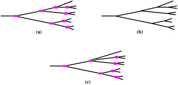
Figure 1: (a) A depiction of a high-energy particle showering in a medium as it moves from left to right. The magenta ovals crudely depict the formation lengths (transversely as well as longitudinally) associated with each splitting. We show here a case where consecutive splittings are well separated compared to formation times [see text]. (b) A corresponding depiction of the approximation made in a simple idealized Monte Carlo (IMC), where the formation times are treated as effectively zero. (c) shows the case where two consecutive splittings (colored magenta and green) happen to overlap. In all of these figures, we have exaggerated the transverse direction: for high-energy particles (and high-energy daughters), splittings will be very nearly collinear.

We want to compute how to account for what happens when two of the splittings are close enough that formation times overlap, such as in fig. 1c, in which case the idealized Monte Carlo assumption that the splittings are independent breaks down. Let’s ignore very-soft bremsstrahlung for now, since it is more-democratic splittings that naively dominate energy loss; the (nonetheless important) effects of very-soft bremsstrahlung have been treated elsewhere Blaizot ; Iancu ; Wu . So imagine that in each splitting the daughters both carry a non-negligible fraction of the parent’s energy. In this case, the separation between splittings is on average large compared to the formation times, provided that $\alpha_{\rm s}$ (evaluated at the scale that characterizes high-energy splittings) is small. The chances that three or more consecutive (democratic) splittings happen to occur with overlapping formation times is then even smaller than the chance that two consecutive splittings overlap. So, to compute the effect of overlapping formation times, it is enough to focus on two consecutive collisions.

A cartoon of the corresponding correction is given in fig. 2. Let $\delta H$ be the part of the Hamiltonian of the theory that includes the splitting vertices for high-energy particles. The first term on the right of fig. 2 represents a calculation of the double-bremsstrahlung rate $d\Gamma/dx\,dy$ in medium, where we have formally expanded to second order in $\delta H$, even though the real-world situation may be that there are eventually many more splittings (such as in fig. 1c). The other terms, subtracted on the right-hand side of fig. 2, represent the result $(d\Gamma/dx\,dy)_{\rm IMC}$ that one would obtain from an idealized Monte Carlo if one formally expanded that result to second order in the splitting probability. (More on what we mean by that in a moment.) Individually, both $d\Gamma/dx\,dy$ and $(d\Gamma/dx\,dy)_{\rm IMC}$ receive contributions from consecutive splittings that are separated in time by much more than the formation times, but those contributions cancel in the difference, as depicted pictorially in fig. 3. Indeed, individually, both $d\Gamma/dx\,dy$ and $(d\Gamma/dx\,dy)_{\rm IMC}$ as defined above would be formally infinite in the case of an infinite medium. (More on that in a moment as well.) In contrast, the result for

$$\Delta\,\frac{d\Gamma}{dx\,dy}\equiv\frac{d\Gamma}{dx\,dy}-\left[\frac{d\Gamma}{dx\,dy}\right]_{\rm IMC}$$ (1)

is finite and depends only on separations $\lesssim$ the relevant formation time.

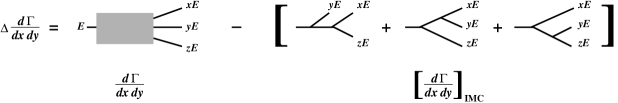
Figure 2: A pictorial version of the definition of $\Delta\,d\Gamma/dx\,dy$ as the difference between (i) the double-splitting rate (represented by the gray box) and (ii) the comparable rate given by idealized Monte Carlo (IMC) restricted to two splittings. Above, $z\equiv 1{-}x{-}y$.

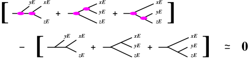
Figure 3: A pictorial summary of the cancellation of the contributions to fig. 2 for splittings that are well-separated in time.

I.1.2 Some simple analogies

Since the above points are important, we will try to illuminate them with some analogies. First, as a warm-up, consider the decay of a particle in quantum mechanics. The generic way to compute the decay rate is to formally compute the probability $P$ for decay, to first order in the process that causes the decay. One finds a result that formally grows proportional to the total time $\mathbb{T}$ as $P=\Gamma\,\mathbb{T}$, from which we extract the rate $\Gamma$. But of course the probability of decay can’t really be $P=\Gamma\,\mathbb{T}$ because that probability would exceed 1 for large enough $\mathbb{T}$. Instead, the probability is $P=1-e^{-\Gamma\mathbb{T}}$. The formula $P=\Gamma\,\mathbb{T}$ is analogous to what we mean above when we say to formally compute or expand a result to a given order in perturbation theory. This example is a rough analogy to constructing an idealized Monte Carlo based on the single bremsstrahlung rate: $\Gamma$ is analogous to the single bremsstrahlung rate, whereas the result $P=1-e^{-\Gamma\mathbb{T}}$ is analogous to what you would get if you actually used a result for $\Gamma$ in an idealized Monte Carlo (as opposed to discussing an idealized Monte Carlo result that had been “formally expanded” to some fixed order in perturbation theory). Let’s now turn to an example that is more analogous to our double bremsstrahlung problem.

Consider the classical analogy of a very tiny device (“particle”) that has a certain probability $\Gamma_{1}$ per unit time of emitting a flash of light. If we formally expand to first order in $\Gamma_{1}$, then the probability of emitting exactly one flash of light in time $\mathbb{T}$ is (formally) $P_{1}=\Gamma_{1}\mathbb{T}$. If we formally expand to second order in $\Gamma_{1}$, then the probability of emitting exactly two flashes of light in time $\mathbb{T}$ is $P_{2}=\frac{1}{2}(\Gamma_{1}\mathbb{T})^{2}$. If we naively divided $P_{2}$ by $\mathbb{T}$ to get a rate, then we would awkwardly say that the rate for two flashes is $\Gamma_{2}=\tfrac{1}{2}\Gamma_{1}^{2}\mathbb{T}$, which (unlike $\Gamma_{1}=P_{1}/\mathbb{T}$) diverges as $\mathbb{T}\to\infty$. So the “rate for two flashes” (analogous to the $d\Gamma/dx\,dy$ for double splitting) is not, by itself, a very meaningful quantity.

But now suppose that the device had the additional property that, for some interval $\delta t$ after emitting one flash, the rate for emitting another flash was temporarily changed to $\Gamma_{1}+\delta\Gamma$. We might then ask for the correction to the previous result. We could again formally expand to second order in flash rates (which are now correlated as just described) to find the probability $P_{2}$ in this new situation, which would roughly have the form $P_{2}=\tfrac{1}{2}(\Gamma_{1}\mathbb{T})^{2}+\Gamma_{1}\,\delta\Gamma\,\delta t\,\mathbb{T}$. If we divided by $\mathbb{T}$ to define a $\Gamma_{2}=\tfrac{1}{2}\Gamma_{1}^{2}\mathbb{T}+\Gamma_{1}\,\delta\Gamma\,\delta t$, we would again have something ill-defined as $\mathbb{T}\to\infty$. However, the correction to $\Gamma_{2}$ due to the change is perfectly well defined as $\Delta\Gamma_{2}\equiv\Gamma_{2}-\tfrac{1}{2}\Gamma_{1}^{2}\mathbb{T}=\Gamma_{1}\,\delta\Gamma\,\delta t$. In this analogy, $\Gamma_{2}$ is like our double-bremsstrahlung rate $d\Gamma/dx\,dy$; $\frac{1}{2}\Gamma_{1}^{2}\mathbb{T}$ is like $(d\Gamma/dx\,dy)_{\rm IMC}$; $\delta t$ is like the formation time; and the correction $\Delta\Gamma_{2}$ is like the $\Delta\,d\Gamma/dx\,dy$ of (1).

To further illuminate the importance and relevance of the subtraction (1), we will present in a moment an analogy with the importance of similar subtractions in kinetic theory. But it will be useful to first discuss what one should do with (1) once one has calculated it.

I.1.3 Uses

What can one do with a calculation of the correction $\Delta\,d\Gamma/dx\,dy$? First note that its definition (1) is as a difference of two positive quantities. A priori, that difference might have either sign: negative if the effect of overlapping formation times suppresses the double bremsstrahlung rate and positive if it enhances it.

If the correction is positive, there is a relatively easy way to implement the correction to an idealized Monte Carlo simulation: Simply interpret $\Delta\,d\Gamma/dx\,dy$ as the probability distribution of an additional type of local splitting process that “instantly” produces three daughters (instead of just two daughters) from one parent. This would allow for Monte Carlo showers such as fig. 4. In contrast, if $\Delta\,d\Gamma/dx\,dy$ is negative, one has to work harder. (Examples in the context of relativistic heavy ion collisions: the Monte Carlo generators JEWEL JEWEL and MARTINI Martini implement heuristic models for a reduction in multiple-splitting rates due to overlapping formation times.)

Figure 4: An example of a process in a corrected Monte Carlo that could easily be implemented if $\Delta\,d\Gamma/dx\,dy$ is positive. Here, the $1\to 3$ splitting, representing the inclusion of an additional possible process in the Monte Carlo with probability distribution $\Delta\,d\Gamma/dx\,dy$, would account for the correction due to the possibility of fig. 1c.

In this paper, we focus on the calculation of $\Delta\,d\Gamma/dx\,dy$ and will not pursue how to incorporate it into Monte Carlo. The earlier discussion of (uncorrected) idealized Monte Carlo was necessary, however, for the definition (1) of $\Delta\,d\Gamma/dx\,dy$. We will discuss the sign of the correction shortly, when presenting numerical results in section I.3.

I.1.4 A kinetic theory analogy

The same issues that lead to focusing on $\Delta\Gamma$ rather than $\Gamma$ (for higher-order processes) arise in kinetic theory problems as well. We start by briefly reviewing a kinetic theory example from the literature. Then we’ll give an example more closely analogous to our double bremsstrahlung problem (and to our earlier flashing device analogy).

Consider a kinetic theory discussion of the following simple model, analyzed by Kolb and Wolfram KolbWolfram in the context of baryogenesis in grand unified theories. The toy model has a stable, nearly-massless particle $b$ and a massive, unstable boson $X$ which can decay by both $X\to bb$ and $X\to\bar{b}\bar{b}$, as depicted in fig. 5. If one writes a kinetic theory for these particles, one would include the processes of fig. 5 (and their inverses) in the collision term. Now consider additionally including the process $bb\to X\to\bar{b}\bar{b}$, depicted in fig. 6a. There is a problem of double counting because the Feynman diagram for $bb\to X\to\bar{b}\bar{b}$ includes two different types of physical processes. One of these is the case where the intermediate $X$ boson is approximately on shell, which we depict by fig. 6b. The other is what’s left: the case where the $X$ boson is off-shell, which we depict in fig. 6c with an asterisk on the label $X$. The first case (fig. 6b) is already accounted for by solving kinetic theory using a collision term based of fig. 5, and so supplementing the collision term by the full result of fig. 6a would double count the case of on-shell $X$. Instead, the collision term should contain just (i) fig. 5 and (ii) the off-shell contribution of fig. 6c. How precisely does one define the “off-shell” part of the contribution? By rearranging the terms of fig. 6 to make it a definition, as in fig. 7. This subtraction is (crudely) analogous to our problem’s subtraction (1). The fact that fig. 7 and not fig. 6a is the correct thing to use in the collision term in Kolb and Wolfram’s problem is analogous to our discussion of adding $\Delta\,d\Gamma/dx\,dy$ rather than $d\Gamma/dx\,dy$ to a Monte Carlo description originally based on single-splitting rates, as in fig. 4.

Figure 5: A depiction of decay processes $X\to bb$ and $X\to\bar{b}\bar{b}$ for our first kinetic theory analogy, based on ref. KolbWolfram .

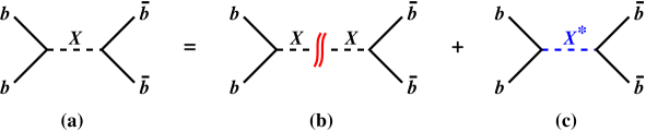
Figure 6: A depiction of (a) the process $bb\to X\to\bar{b}\bar{b}$ separated into contributions (b) where the $X$ is on-shell plus (c) the rest. The wavy double-line cut in the middle of (b) is used to indicate that the intermediate particle $X$ is on-shell.

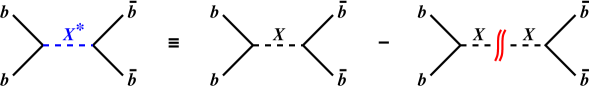
Figure 7: Reorganization of fig. 6 to show the subtracted quantity that should be used in the collision term of a kinetic theory analysis.

We now give a kinetic theory example that is somewhat more analogous to the current problem. Ignore the LPM effect, but consider a kinetic theory description of a QED plasma that includes the leading-order, $2{\to}3$ process for bremsstrahlung, depicted by fig. 8. What if we now want to systematically include higher-order processes in the collision term? Consider in particular the $3{\to}5$ process depicted in fig. 9a. Just like fig. 6, this process contains two types of contributions. Including the contribution with an on-shell intermediate line, depicted by fig. 9b, would be double counting. Instead, one should only add to the collision term the remaining piece, fig. 9c, which is defined as the difference between figs. 9a and 9b. Here, figs. 9a, b, and c are analogous to our problem’s $d\Gamma/dx\kern 1.0ptdy$, $[d\Gamma/dx\kern 1.0ptdy]_{\rm IMC}$, and $\Delta\,d\Gamma/dx\kern 1.0ptdy$ respectively.

Figure 8: A depiction of the leading-order bremsstrahlung process that could be used in the collision term for a kinetic theory description of a QED plasma, in cases where the LPM effect can be ignored. (There are other Feynman diagrams that contribute to this process at this order, but we just show the one for simplicity.)

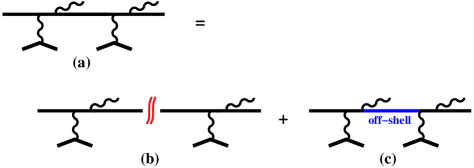
Figure 9: A depiction of (a) double bremsstrahlung in the kinetic theory example of fig. 8, separated into contributions (b) where the intermediate particle is on-shell plus (c) the rest.

These are not perfect analogies (they do not involve the LPM effect), but we hope they help illuminate the importance of the subtraction (1).

I.2 What we compute (and what we do not)

The preceding work 2brem developed most of the formalism we will need for carrying out calculations and then (in approximations reviewed below) computed the subset of contributions to the double-bremsstrahlung rate depicted in fig. 10. It is very convenient to alternatively represent these contributions as in fig. 11, where the upper (blue) part of the diagrams depict a contribution to the amplitude and the lower (red) part depict a contribution to the conjugate amplitude. Ref. 2brem referred to these as the “crossed” contributions to the rate because the interior lines are crossed in the representations of fig. 11. In both figs. 10 and 11, we explicitly show only the high-energy particles; the (many) interactions of those high-energy particles with the medium are implicit. (See the introduction of ref. 2brem for more description.)

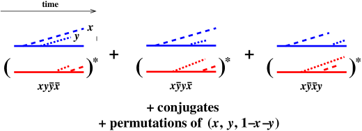
Figure 10: The subset of interference contributions to double splitting previously evaluated in ref. 2brem : the “crossed” diagrams. To simplify the drawing, all particles, including bremsstrahlung gluons, are indicated by straight lines. The long-dashed and short-dashed lines are the daughters with momentum fractions $x$ and $y$ respectively. The naming of the diagrams indicates the time order in which emissions occur in the amplitude and conjugate amplitude. For instance, $x\bar{y}y\bar{x}$ means first (i) $x$ emission in the amplitude, then (ii) $y$ emission in the conjugate amplitude, then (iii) $y$ emission in the amplitude, and then (iv) $x$ emission in the conjugate amplitude.

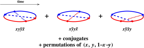
Figure 11: An alternative depiction of fig. 10, with amplitudes (blue) and conjugate amplitudes (red) sewn together. The dashed lines are colored according to whether they were first emitted in the amplitude or conjugate amplitude.

In this paper, we will now evaluate the diagrams of figs. 12 and 13, which we refer to as “sequential” contributions because the two bremsstrahlung emissions happen in the same order in both the amplitude and conjugate amplitude. To compute the desired correction $\Delta\,d\Gamma/dx\,dy$ to double bremsstrahlung due to overlapping formation times, we will need to subtract from our results the naive calculation of double bremsstrahlung as two consecutive, quantum-mechanically independent splitting processes, as in (1). In the last two diagrams ($x\bar{x}y\bar{y}$ and $x\bar{x}\bar{y}y$) of figs. 12 and 13, the $x$ and $y$ bremsstrahlung processes do not overlap in time. We will see later that these diagrams roughly, but not quite, match up with the idealized Monte Carlo calculation. Figuring out how to correctly compute the difference will be the main new technical development required for this paper.

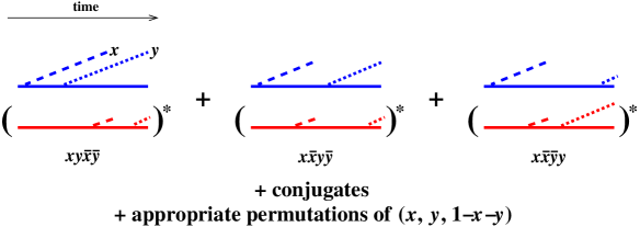
Figure 12: The interference contributions evaluated in this paper: the “sequential” diagrams.

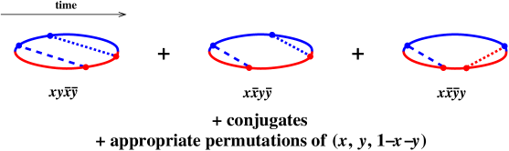
Figure 13: An equivalent representation of fig. 12.

As discussed in the preceding work 2brem , it is possible to set up the formalism in a quite general way that would require both highly non-trivial numerics and a non-trivial treatment of color dynamics to implement, but one can proceed much further analytically by making a few additional approximations. Though the methods we will discuss in this paper can be applied more generally, it behooves us to keep things simple in this first treatment. So we will follow ref. 2brem when it comes to explicit calculations, by making the following approximations.

• We will assume that the medium is static, uniform and infinite (which in physical terms means approximately uniform over the formation time and corresponding formation length).

• We take the large-$N_{\rm c}$ limit of QCD to simplify the color dynamics. [The specialization of our general result for $\Delta\,d\Gamma/dx\,dy$ to the soft limiting case $y\ll x\ll 1$ will not depend on this assumption.]

• We make the multiple-scattering approximation to interactions with the medium, appropriate for very high energies and also known as the harmonic oscillator or $\hat{q}$ approximation.

Also as in ref. 2brem , we will focus on the case where the initial high-energy particle is a gluon (and so, in large-$N_{\rm c}$, the final high-energy particles are also all gluons), as the resulting final-state permutation symmetries make for fewer diagrams to consider so far. However, there is a downside. In the case of gluons, one must also consider the 4-gluon interaction, which gives rise to additional interference contributions. Examples are given in fig. 14. Because the calculation of these additional diagrams would distract from the main point of this paper, which is how to treat the sequential diagrams in the calculation of $\Delta d\Gamma/dx\,dy$, we will leave fig. 14 for future work 4point . It turns out that these contributions are small whenever at least one of the three final gluons is soft, so the still-incomplete results that we derive here will have some range of applicability. But we will need fig. 14 for a complete calculation for the case of arbitrary $x$ and $y$.

Figure 14: Examples of interference contributions involving 4-gluon vertices. Such contributions are not evaluated in this paper but will be needed for a complete calculation of double bremsstrahlung from an initial gluon for arbitrary $x$ and $y$.

Another problem that we defer for another time is the change in the single-bremsstrahlung rate due to virtual corrections, such as the one shown in fig. 15. This has been worked out in the limiting case $y\ll x\ll 1$ in the context of leading parton average energy loss in refs. Blaizot ; Iancu ; Wu and is related to anomalous scaling of the effective medium parameter $\hat{q}$ with energy.

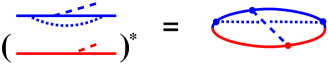
Figure 15: An example of a virtual loop correction to single splitting.

Finally, we should mention that the relative transverse momentum of daughters immediately following a double-splitting has been integrated in our results. Though we will make some qualitative comments regarding transverse momenta later on, we have not calculated transverse momentum distributions. (If we did not integrate the double-splitting rate over transverse momenta, the calculation would be much harder, including the necessity of accounting for decaying color coherence effects Blaizot0 occurring after the last splitting time in, for example, each of the diagrams of fig. 10. See appendix F for a brief discussion.)

I.3 Preview of Results

Numerical results are given in fig. 16 for the sum of the crossed and sequential contributions to the correction $\Delta\,\Gamma/dx\,dy$ for real double gluon bremsstrahlung from an initial gluon. As mentioned above, the effects of 4-gluon vertices (such as in fig. 14) have not yet been included. We do not expect these to be important when one of the final gluons is soft, and so we can already draw the conclusion from fig. 16 that sometimes the correction $\Delta\,\Gamma/dx\,dy$ is positive and sometimes it is negative, with the corresponding implications for the relative ease or difficulty of Monte Carlo implementation discussed earlier at the end of section I.1. However, as a pragmatic matter, note from the figure that one final gluon has to have about 10 times smaller energy than the other two in order to get a negative correction. So, if one did implement a correction to real double bremsstrahlung in Monte Carlo, the most important effects for shower development (that are not simply absorbable into the running of $\hat{q}$ from soft emissions as discussed in Blaizot ; Iancu ; Wu ) may correspond to the cases of positive correction, which is the more straightforward case to implement. However, the most interesting region is where all three final gluons carry substantial momentum fractions, and for that case we will need those 4-gluon vertex contributions, which we have left for later work.

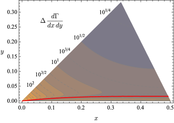
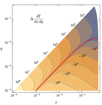
Figure 16: Results for $\Delta\,d\Gamma/dx\,dy$ in units of $C_{\rm A}^{2}\alpha_{\rm s}^{2}(\hat{q}_{\rm A}/E)^{1/2}$, including both crossed and sequential contributions (but not yet the 4-gluon vertex contributions such as fig. 14). Since all three final state particles are gluons and so are identical particles, we only show results for the region $y<x<z\equiv 1{-}x{-}y$. (All other orderings are equivalent by permutation.) The red line shows where the result vanishes, dividing the sub-region of positive corrections from the sub-region of negative corrections.

In the special limiting case of $y\lll x\ll 1$, the numerical results approach

$$\Delta\,\frac{d\Gamma}{dx\,dy}\simeq-0.895\,\frac{C_{\rm A}^{2}\alpha_{\rm s}^{2}}{\pi^{2}xy^{3/2}}\sqrt{\frac{\hat{q}_{\rm A}}{E}}\,.$$ (2)

This result is negative, as in the corresponding region of fig. 16. In a moment, we will give a simple general argument about why $\Delta\,d\Gamma/dx\,dy$ could be expected to scale parametrically like $1/xy^{3/2}$, as above. This scaling suggests that a smoother way to plot our final results, even outside of the $y\ll x\ll 1$ limit, is to pull out a factor of $1/\pi^{2}xy^{3/2}$ from the answer. Fig. 17 presents our results that way. One needs to see a larger range of $y$ to verify the (somewhat slow) approach to the limit (2), which is shown in fig. 18 for a particular, small fixed value of $x$.

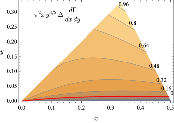
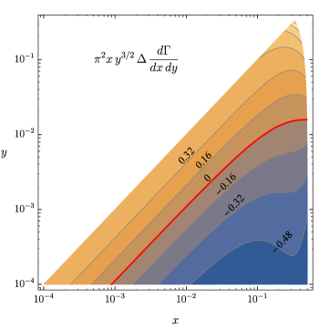
Figure 17: As fig. 16 but removing a factor of $1/(\pi^{2}xy^{3/2})$ from the answer. The apex $(x,y)=(\frac{1}{3},\frac{1}{3})$ of the triangular region above corresponds to $\pi^{2}xy^{3/2}\Delta\,d\Gamma/dx\,dy=1.05$ [in units of $C_{\rm A}^{2}\alpha_{\rm s}^{2}(\hat{q}_{\rm A}/E)^{1/2}$].

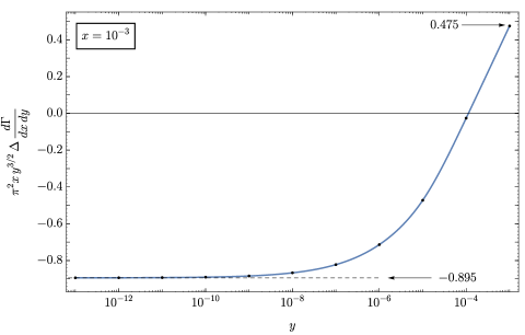
Figure 18: The same result as fig. 17 but showing the $y$ dependence for fixed $x=10^{-3}$.

We should note that the soft limit (2) for the correction $\Delta\,d\Gamma/dx\,dy$ to the double real gluon bremsstrahlung rate cannot be extracted from early work Blaizot ; Iancu ; Wu on soft multiple bremsstrahlung because that work used approximations that are only valid for the sum of (i) real double gluon emission with (ii) virtual corrections to single gluon emission and are not valid for (i) and (ii) individually. Also, our result (2) depends on diagrams that were not evaluated in refs. Blaizot ; Iancu ; Wu , such as the $x\bar{y}\bar{x}y$ diagram of figs. 10 and 11.

The integral formula we will derive for $\Delta\,d\Gamma/dx\,dy$ in the general case is a complicated expression that is painstaking to implement. In Appendix A, we provide, as an alternative, a relatively simple analytic formula that has been fitted to approximate fig. 17 very well.

I.4 Why $1/xy^{3/2}$?

Before moving on to the details of calculations, we give one crude but simple explanation of why the rate for overlapping emissions has parametric dependence $(d\Gamma/dx\,dy)_{\rm overlap}\sim 1/xy^{3/2}$ when $y<x<z\equiv 1{-}x{-}y$.

First, let’s review some features of the LPM effect for the usual case of single bremsstrahlung, with $x$ representing the less energetic of the two daughters. In the QCD case, the formation time for this bremsstrahlung process is (for thick media) parametrically

$$t_{{\rm form},x}\sim\sqrt{\frac{xE}{\hat{q}}}\,.$$ (3)

Each formation time offers one opportunity for splitting, with probability of order $\alpha_{\rm s}$. So the rate for emission of a daughter with momentum fraction of order $x$ is

$$\Gamma_{x}\sim\frac{\alpha_{\rm s}}{t_{{\rm form},x}}\sim\alpha_{\rm s}\sqrt{\frac{\hat{q}}{xE}}\,,$$ (4)

corresponding to

$$\frac{d\Gamma_{x}}{dx}\sim\frac{\alpha_{\rm s}}{xt_{{\rm form},x}}\sim\frac{\alpha_{\rm s}}{x}\,\sqrt{\frac{\hat{q}}{xE}}\,.$$ (5)

Now consider double bremsstrahlung with $y<x$. From (3), the $y$ formation time will be shorter than the $x$ formation time. The probability that an emission with momentum fraction of order $y$ happens during the $x$ formation time $t_{{\rm form},x}$ is then given by

$$\Gamma_{y}\,t_{{\rm form},x}\sim\frac{\alpha_{\rm s}}{t_{{\rm form},y}}\,t_{{\rm form},x},$$ (6)

corresponding to

$$\frac{d\Gamma_{y}}{dy}\,t_{{\rm form},x}\sim\frac{\alpha_{\rm s}}{yt_{{\rm form},y}}\,t_{{\rm form},x}.$$ (7)

Multiplying (5) and (7) gives the rate for overlapping $x$ and $y$ emissions:

$$\left[\frac{d\Gamma}{dx\,dy}\right]_{\rm overlap}\sim\frac{d\Gamma_{x}}{dx}\times\frac{d\Gamma_{y}}{dy}\,t_{{\rm form},x}\sim\frac{\alpha_{\rm s}^{2}}{xyt_{{\rm form},y}}\sim\frac{\alpha_{\rm s}^{2}}{xy^{3/2}}\sqrt{\frac{\hat{q}}{E}}\,.$$ (8)

If the presence of the $y$ emission has a significant effect on the $x$ emission (or vice versa), then the correction $\Delta\,d\Gamma/dx\,dy$ defined by (1) would then also be

$$\Delta\,\frac{d\Gamma}{dx\,dy}\sim\frac{\alpha_{\rm s}^{2}}{xy^{3/2}}\sqrt{\frac{\hat{q}}{E}}\,.$$ (9)

This is indeed the parametric behavior (2) of our result in this paper. It turns out that, separately, the crossed and sequential diagrams are each logarithmically enhanced,

$$\left[\frac{d\Gamma}{dx\,dy}\right]_{\rm crossed}\sim\left[\Delta\frac{d\Gamma}{dx\,dy}\right]_{\rm sequential}\sim\frac{\alpha_{\rm s}^{2}}{xy^{3/2}}\sqrt{\frac{\hat{q}}{E}}\,\ln\left(\frac{x}{y}\right)$$ (10)

for $y\ll x\ll 1$, but the logarithmically-enhanced contributions cancel each other in the total (9). Appendix B discusses how the logarithmic enhancement of various individual contributions can be related to collinear logarithms from DGLAP evolution and fragmentation, and how there is a Gunion-Bertsch-like GB cancellation of those logarithms in the total result. This is not to say that collinear logarithms are never relevant, just that they do not appear at the order $\alpha_{\rm s}^{2}/xy^{3/2}$ of (9). They do appear, notably, in calculations Blaizot ; Iancu ; Wu of energy loss. In that case, the effect of the leading contribution (9) to energy loss from double bremsstrahlung is canceled by the leading contribution from virtual corrections to the single bremsstrahlung rate, and so it is the sub-leading behavior of each which becomes important.

Finally, note using (3) that the total probability (6) of emitting a $y$ during the formation time of $x$ is of order

$$\Gamma_{y}\,t_{{\rm form},x}\sim\alpha_{\rm s}\sqrt{\frac{x}{y}}.$$ (11)

So one would need to deal with resumming multiple $O(y)$ emissions during the $x$ formation time if interested in $y\lesssim\alpha_{\rm s}^{2}x$. We will not treat that case in this paper. (When discussing the mathematical behavior of our results, we will nonetheless discuss some absurdly small values of $y$, such as in fig. 18. Our results for such small $y$ directly apply only to the formal limit that the $\alpha_{\rm s}$ associated with splitting is arbitrarily small.)

II The Calculation

In this section, we turn to the specifics of calculating the sequential diagrams of fig. 13. The first interference diagram in the figure, $xy\bar{x}\bar{y}$, can be evaluated by mostly-straightforward application of the methods of the preceding work 2brem . We will leave the details for later, in section II.2 and appendix E. The only new subtlety of this diagram, as opposed to the crossed diagrams evaluated in ref. 2brem , is that there are two inequivalent ways that color can be routed in the large-$N_{\rm c}$ approximation, which must be accounted for appropriately.

To begin, we will instead focus on the other explicit diagrams of fig. 13, $x\bar{x}y\bar{y}+x\bar{x}\bar{y}y$, as these are the diagrams that involve the most significant new issue: careful attention to the subtraction of $(d\Gamma/dx\,dy)_{\rm IMC}$ from $d\Gamma/dx\,dy$.

II.1 $2\operatorname{Re}(x\bar{x}y\bar{y}+x\bar{x}\bar{y}y)$ vs. idealized Monte Carlo

Start by considering $x\bar{x}y\bar{y}$. Our convention for labeling time in this diagram is shown in fig. 19. Following the philosophy of the preceding paper 2brem , we may interpret the evolution between vertex times to be described by 2-dimensional non-relativistic non-Hermitian quantum mechanics, with the appropriate number of particles. In the case of fig. 19, it is a (i) 3-particle problem for $t_{\rm x}<t<t_{\bar{\rm x}}$, (ii) 2-particle problem for $t_{\bar{\rm x}}<t<t_{\rm y}$, and (iii) 3-particle problem for $t_{\rm y}<t<t_{\bar{\rm y}}$. Also following ref. 2brem , we may use symmetry to reduce the $N$ particle problems to $(N{-}2)$ particle problems, leaving us with (i) 1-particle, (ii) 0-particle, and (iii) 1-particle problems respectively.

Figure 19: The $x\bar{x}y\bar{y}$ interference, showing longitudinal momentum fractions $x_{i}$ and our notation for the vertex times.

At this point, we could implement the methods of the preceding paper 2brem to turn fig. 19 into explicit equations and then start turning the crank. We do this in appendix C for the sake of concreteness. However, many of these details can be sidestepped if we take a slightly looser approach, which is how we will proceed here in the main text.

The important point is that, for the $x\bar{x}y\bar{y}$ diagram of fig. 19 (and similarly for the $x\bar{x}\bar{y}y$ diagram in fig. 13), the time interval $(t_{\rm x},t_{\bar{\rm x}})$ of the $x$ emission does not overlap with the time interval $(t_{\rm y},t_{\bar{\rm y}})$ of the $y$ emission. So the times of these events are unrelated—there is no reason the $y$ emission cannot occur a very long time after the $x$ emission. In the formalism, this is because evolution during the intermediate time interval $t_{\bar{\rm x}}<t<t_{\rm y}$ corresponds to a problem with effectively zero particles and so does not have any time dependence: the $x\bar{x}y\bar{y}$ interference contribution does not care how far apart $t_{\bar{\rm x}}$ and $t_{\rm y}$ are. This is consistent with interpreting this diagram as representing two consecutive splittings that are completely independent from each other, as in an idealized Monte Carlo calculation.

II.1.1 A crude correspondence

In particular, the $x\bar{x}y\bar{y}+x\bar{x}\bar{y}y$ cases (plus conjugates) in figs. 12 and 13 are related to the idealized Monte Carlo contribution of fig. 20, where a first splitting, $E\to(1{-}x)E$ and $xE$, is followed later by an independent second splitting, $(1{-}x)E\to zE$ and $yE$. In what follows, it will be convenient to introduce the longitudinal momentum fraction ${\mathfrak{y}}$ of the $y$ daughter with respect to its immediate parent in the second splitting,

$${\mathfrak{y}}\equiv\frac{y}{1-x}\,.$$ (12)

That is, the $y$ daughter has energy $yE={\mathfrak{y}}(1-x)E$. In the language that we use for labeling diagrams, single-splitting rates are given by $2\operatorname{Re}(x\bar{x})=x\bar{x}+\bar{x}x$, with $x\bar{x}$ depicted in fig. 21. The correspondence here between double-splitting diagrams and Monte Carlo is, crudely speaking,

$$\left[\frac{d\Gamma}{dx\,d{\mathfrak{y}}}\right]_{\begin{subarray}x\bar{x}y\bar{y}+x\bar{x}\bar{y}y\\ +\bar{x}x\bar{y}y+\bar{x}xy\bar{y}\end{subarray}}\approx\left[\frac{d\Gamma}{dx\,d{\mathfrak{y}}}\right]_{\rm corresponding~{}IMC}=\left[\frac{d\Gamma}{dx}\right]_{E}\times\mathbb{T}\,\left[\frac{d\Gamma}{d{\mathfrak{y}}}\right]_{(1-x)E},$$ (13)

where $\mathbb{T}$ formally represents the amount of time between the first splitting and the end of eternity (a regularization that we will soon have to treat more carefully). The right-hand side of (13) is the single-splitting rate $[d\Gamma/dx]_{E}$ for the first splitting (the $x$ emission) times the single-splitting probability $\mathbb{T}\,[d\Gamma/d{\mathfrak{y}}]_{(1-x)E}$ for the second splitting ($y$ emission). The subscripts $E$ and $(1-x)E$ on the single-splitting rates indicate the energy of the parent. Using (12), the rate (13) can be recast in the form

$$\left[\frac{d\Gamma}{dx\,dy}\right]_{\begin{subarray}x\bar{x}y\bar{y}+x\bar{x}\bar{y}y\\ +\bar{x}x\bar{y}y+\bar{x}xy\bar{y}\end{subarray}}\approx\left[\frac{d\Gamma}{dx\,dy}\right]_{\rm corresponding~{}IMC}=\frac{\mathbb{T}}{1-x}\,\left[\frac{d\Gamma}{dx}\right]_{E}\,\left[\frac{d\Gamma}{d{\mathfrak{y}}}\right]_{(1-x)E}.$$ (14)

As in the earlier discussion in section I.1, the infinite quantity $\mathbb{T}$ will only make a temporary appearance along the way towards finding the correction $\Delta\,d\Gamma/dx\,dy$ to idealized Monte Carlo.

Figure 20: Idealized Monte Carlo contribution related to $x\bar{x}y\bar{y}+x\bar{x}\bar{y}y+\bar{x}x\bar{y}y+\bar{x}xy\bar{y}=2\operatorname{Re}(x\bar{x}y\bar{y}+x\bar{x}\bar{y}y)$.

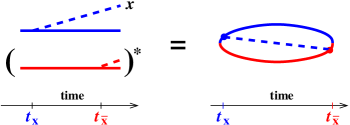
Figure 21: The $x\bar{x}$ interference contribution to single splitting.

Let’s now use some more explicit formulas for the single-splitting rates appearing on the right-hand side of (14). In notation similar to that of the preceding paper 2brem ,

$$\left[\frac{d\Gamma}{dx}\right]_{E}=\frac{\alpha P(x)}{[x(1-x)E]^{2}}\operatorname{Re}\int_{0}^{\infty}d(\Delta t)\>{\bm{\nabla}}_{{\bm{B}}^{\bar{\rm x}}}\cdot{\bm{\nabla}}_{{\bm{B}}^{\rm x}}\langle{\bm{B}}^{\bar{\rm x}},\Delta t|{\bm{B}}^{\rm x},0\rangle_{E,x}\Bigr{|}_{{\bm{B}}^{\bar{\rm x}}={\bm{B}}^{\rm x}=0},$$ (15)

corresponding to twice the real part of the $x\bar{x}$ diagram for single splitting, shown in fig. 21. The $x\bar{x}$ contribution alone is

$$\left[\frac{d\Gamma}{dx}\right]_{x\bar{x},E}=\frac{\alpha P(x)}{2[x(1-x)E]^{2}}\int_{0}^{\infty}d(\Delta t)\>{\bm{\nabla}}_{{\bm{B}}^{\bar{\rm x}}}\cdot{\bm{\nabla}}_{{\bm{B}}^{\rm x}}\langle{\bm{B}}^{\bar{\rm x}},\Delta t|{\bm{B}}^{\rm x},0\rangle_{E,x}\Bigr{|}_{{\bm{B}}^{\bar{\rm x}}={\bm{B}}^{\rm x}=0}.$$ (16)

Here, $P(x)$ is the relevant (helicity-averaged) DGLAP splitting function. ${\bm{B}}$ is the single transverse position associated with the “effectively 1-particle” description of this process. The subscripts at the end of $\langle{\bm{B}}^{\bar{\rm x}},\Delta t|{\bm{B}}^{\rm x},0\rangle_{E,x}$ are a reminder (which will be useful in a moment) of what energy and branching fraction should be used in the calculation of the propagator for ${\bm{B}}$. The integration variable $\Delta t$ in (15) represents the time difference $t_{\bar{\rm x}}-t_{\rm x}$ in fig. 21. We will later give more explicit formulas for (15) in the multiple scattering ($\hat{q}$) approximation, but for the moment there is no reason not to be general. To simplify notation in what follows, we will rewrite (15) generically as

$$\left[\frac{d\Gamma}{dx}\right]_{E}=\operatorname{Re}\int_{0}^{\infty}d(\Delta t)\>\left[\frac{d\Gamma}{dx\,d(\Delta t)}\right]_{E}\,,$$ (17)

where the complex-valued $d\Gamma/dx\,d(\Delta t)$ is defined by

$$\left[\frac{d\Gamma}{dx\,d(\Delta t)}\right]_{E}\equiv\frac{\alpha P(x)}{[x(1-x)E]^{2}}{\bm{\nabla}}_{{\bm{B}}^{\bar{\rm x}}}\cdot{\bm{\nabla}}_{{\bm{B}}^{\rm x}}\langle{\bm{B}}^{\bar{\rm x}},\Delta t|{\bm{B}}^{\rm x},0\rangle_{E,x}\Bigr{|}_{{\bm{B}}^{\bar{\rm x}}={\bm{B}}^{\rm x}=0}.$$ (18)

Putting the integral form (17) of the single bremsstrahlung rate into the right-hand side of (14), we can write the idealized Monte Carlo result for double bremsstrahlung as

$$\left[\frac{d\Gamma}{dx\,dy}\right]_{\rm corresponding~{}IMC}=\frac{\mathbb{T}}{(1-x)} \int_{0}^{\infty}d(\Delta t_{\rm x})\int_{0}^{\infty}d(\Delta t_{\rm y})$$

$$\times\operatorname{Re}\left[\frac{d\Gamma}{dx\,d(\Delta t_{\rm x})}\right]_{E}\,\operatorname{Re}\left[\frac{d\Gamma}{d{\mathfrak{y}}\,d(\Delta t_{\rm y})}\right]_{(1-x)E}$$ (19)

with the interpretations

$$\Delta t_{\rm x}\equiv|t_{\bar{\rm x}}-t_{\rm x}|\quad\mbox{and}\quad\Delta t_{\rm y}\equiv|t_{\bar{\rm y}}-t_{\rm y}|.$$ (20)

As we verify explicitly in appendix C, the above idealized Monte Carlo contribution corresponds to the result for the diagrams $x\bar{x}y\bar{y}+x\bar{x}\bar{y}y+\bar{x}x\bar{y}y+\bar{x}xy\bar{y}=2\operatorname{Re}(x\bar{x}y\bar{y}+x\bar{x}\bar{y}y)$, with one critically important difference. To explain that difference, look at the piece of (19) corresponding just to $x\bar{x}$ followed by $y\bar{y}$ [as opposed to the full $2\operatorname{Re}(x\bar{x})=x\bar{x}+\bar{x}x$ followed by $2\operatorname{Re}(y\bar{y})=y\bar{y}+\bar{y}y$]:

$$\left[\frac{d\Gamma}{dx\,dy}\right]_{\begin{subarray}\rm IMC~{}corresponding\\ to~{}x\bar{x}y\bar{y}\ \end{subarray}}=\frac{\mathbb{T}}{1-x} \int_{0}^{\infty}d(\Delta t_{\rm x})\int_{0}^{\infty}d(\Delta t_{\rm y})$$

$$\times\frac{1}{2}\left[\frac{d\Gamma}{dx\,d(\Delta t_{\rm x})}\right]_{E}\,\frac{1}{2}\left[\frac{d\Gamma}{d{\mathfrak{y}}\,d(\Delta t_{\rm y})}\right]_{(1-x)E}.$$ (21)

The actual result from the $x\bar{x}y\bar{y}$ diagram is the same except for the constraints on the time integration in fig. 19:

$$\mathbb{T}\int_{0}^{\infty}\!d(\Delta t_{\rm x})\int_{0}^{\infty}\!d(\Delta t_{\rm y})\>\cdots\qquad$$ in (21)

$$\longrightarrow\quad\int_{t_{\rm x}<t_{\bar{\rm x}}<t_{\rm y}<t_{\bar{\rm y}}}\!dt_{\bar{\rm x}}\,dt_{\rm y}\,dt_{\bar{\rm y}}\>\cdots\qquad x\bar{x}y\bar{y}$$ in (fig. 19). (22)

(There are only three time integrals on the right-hand side because of our focus on computing rates rather than probabilities in this paper, and our associated assumption of time translation invariance over relevant time scales.)

If we are sloppy, we might be tempted to conclude that these two types of time integrations are the same by (i) rewriting the right-hand side of (22) as

$$\int_{0}^{\infty}\!d(t_{\bar{\rm x}}-t_{\rm x})\int_{0}^{\infty}\!d(t_{\rm y}-t_{\bar{\rm x}})\int_{0}^{\infty}\!d(t_{\bar{\rm y}}-t_{\rm y})\>\cdots;$$ (23)

(ii) noticing that the integrand in (21) does not depend on $t_{\rm y}-t_{\bar{\rm x}}$, just as previously discussed concerning the propagation of the effectively 0-particle intermediate state in the diagram for $x\bar{x}y\bar{y}$; and so (iii) replacing the $\int d(t_{\rm y}-t_{\bar{\rm x}})$ in (23) by $\mathbb{T}$ to get the left-hand side of (22). The last step is not quite correct, however, because the maximum allowed duration of the intermediate time interval $(t_{\bar{\rm x}},t_{\rm y})$ in fig. 19 will depend, for example, on how much of the available time $\mathbb{T}$ is being used up by the following time interval $(t_{\rm y},t_{\bar{\rm y}})$, since $t_{\bar{\rm y}}$ must also occur before the end of eternity. The integrand in (21) will fall off exponentially when the duration $t_{\bar{\rm y}}-t_{\rm y}$ of the last interval becomes large compared to the $y$ emission formation time, and so that interval’s effect on the sloppy result

$$\int_{0}^{\infty}\!d(t_{\rm y}-t_{\bar{\rm x}})\approx\mathbb{T}$$ (24)

is only an edge effect, changing the right-hand side by subtracting an amount of order $\mathbb{T}^{0}$. Such an edge effect would be negligible (relatively speaking) as $\mathbb{T}\to\infty$ were we interested only individually in the formal result for $x\bar{x}y\bar{y}$ or the corresponding idealized Monte Carlo contribution (results which are individually physically nonsensical as $\mathbb{T}\to\infty$). However, we are instead interested in the difference $\Delta\,d\Gamma/dx\,dy$, for which the leading $O(\mathbb{T})$ pieces cancel, leaving behind the $O(\mathbb{T}^{0})$ corrections, which then have a sensible $\mathbb{T}\to\infty$ limit.

We could attempt to proceed by figuring out how to somehow consistently carry through the calculation with a sharp cut-off on time, as we were sloppily considering above. This introduces many headaches. The path of least confusion is to introduce a smooth and physically-realizable cut-off. One regularization method is to imagine a situation where the strength $\hat{q}$ of medium interactions very slowly falls off at large times to reach the vacuum. For example, take

$$\hat{q}(t)=\hat{q}_{0}\,e^{-t^{2}/\mathbb{T}^{2}}.$$ (25)

The prescription that then arises in the $\mathbb{T}\to\infty$ limit turns out to be reasonably intuitive and straightforward to implement.

II.1.2 The prescription

Here, we will state the prescription and use it to find $\Delta\,d\Gamma/dx\,dy$. We leave to appendix D a more thorough justification, based on slowly-varying choices of $\hat{q}(t)$ like (25).

Let $\tau_{x}$ and $\tau_{y}$ be the (instantaneous) times of the $x$ and $y$ emission in the idealized Monte Carlo treatment of fig. 20. When comparing to the the calculation of $2\operatorname{Re}(x\bar{x}y\bar{y}+x\bar{x}\bar{y}y)$, the prescription is to identify these Monte Carlo times with the midpoints of the corresponding time intervals $(t_{\rm x},t_{\bar{\rm x}})$ and $(t_{\rm y},t_{\bar{\rm y}})$ of the emissions. That is,

$$\tau_{x}=\frac{t_{\rm x}+t_{\bar{\rm x}}}{2}\,,\qquad\tau_{y}=\frac{t_{\rm y}+t_{\bar{\rm y}}}{2}\,.$$ (26)

Now remember that the $\mathbb{T}$ in the idealized Monte Carlo formula (13) was just an attempt to regularize the integral

$$\int_{0}^{\infty}d(\tau_{\rm y}-\tau_{\rm x})\approx\mathbb{T}.$$ (27)

Instead of giving that integral a name $\mathbb{T}$, let’s just step back and write this integral in place of $\mathbb{T}$. We can then combine it with the $\Delta t$ integrals in the more explicit idealized Monte Carlo result (21) to recast (21) as

$$\left[\frac{d\Gamma}{dx\,dy}\right]_{\begin{subarray}\rm IMC~{}corresponding\\ to~{}x\bar{x}y\bar{y}\ \end{subarray}}=\frac{1}{1-x} \int_{\tau_{\rm x}<\tau_{\rm y}}\!dt_{\bar{\rm x}}\,dt_{\rm y}\,dt_{\bar{\rm y}}$$

$$\times\frac{1}{2}\left[\frac{d\Gamma}{dx\,d(\Delta t_{\rm x})}\right]_{E}\,\frac{1}{2}\left[\frac{d\Gamma}{d{\mathfrak{y}}\,d(\Delta t_{\rm y})}\right]_{(1-x)E}$$ (28)

with the $\Delta t$’s and $\tau$’s defined here by (20) and (26). In contrast, the result of the $x\bar{x}y\bar{y}$ diagram is given using the integral on the right-hand side of (22),

$$\left[\frac{d\Gamma}{dx\,dy}\right]_{x\bar{x}y\bar{y}}=\frac{1}{1-x} \int_{t_{\rm x}<t_{\bar{\rm x}}<t_{\rm y}<t_{\bar{\rm y}}}\!dt_{\bar{\rm x}}\,dt_{\rm y}\,dt_{\bar{\rm y}}$$

$$\times\frac{1}{2}\left[\frac{d\Gamma}{dx\,d(\Delta t_{\rm x})}\right]_{E}\,\frac{1}{2}\left[\frac{d\Gamma}{d{\mathfrak{y}}\,d(\Delta t_{\rm y})}\right]_{(1-x)E}.$$ (29)

The difference, which contributes to $\Delta\,d\Gamma/dx\,dy$, corresponds to

$$\int_{t_{\rm x}<t_{\bar{\rm x}}<t_{\rm y}<t_{\bar{\rm y}}}\!dt_{\bar{\rm x}}\,dt_{\rm y}\,dt_{\bar{\rm y}}\>\cdots-\int_{\tau_{\rm x}<\tau_{\rm y}}\!dt_{\bar{\rm x}}\,dt_{\rm y}\,dt_{\bar{\rm y}}\>\cdots$$ (30)

which may be reorganized as

$$-\int_{0}^{\infty}\!d(\Delta t_{\rm x})\int_{0}^{\infty}\!d(\Delta t_{\rm y})\int_{\tau_{\rm x}}^{\tau_{\rm x}+\frac{1}{2}(\Delta t_{\rm x}+\Delta t_{y})}\!d\tau_{\rm y}\>\cdots.$$ (31)

The integrand in (28), however, depends only on the $\Delta t$’s and not separately on $\tau_{\rm y}$, so the $d\tau_{\rm y}$ integration in (31) is trivial and leaves

$$-\int_{0}^{\infty}\!d(\Delta t_{\rm x})\int_{0}^{\infty}\!d(\Delta t_{\rm y})\>\tfrac{1}{2}(\Delta t_{\rm x}+\Delta t_{y})\>\cdots.$$ (32)

Letting the notation $[\Delta\,d\Gamma/dx\,dy]_{x\bar{x}y\bar{y}}$ represent the difference between $x\bar{x}y\bar{y}$ and the corresponding piece of the idealized Monte Carlo calculation, (28) becomes

$$\left[\Delta\frac{d\Gamma}{dx\,dy}\right]_{x\bar{x}y\bar{y}}=-\frac{1}{1-x} \int_{0}^{\infty}\!d(\Delta t_{\rm x})\int_{0}^{\infty}\!d(\Delta t_{\rm y})\>\tfrac{1}{2}(\Delta t_{\rm x}+\Delta t_{y})$$

$$\times\frac{1}{2}\left[\frac{d\Gamma}{dx\,d(\Delta t_{\rm x})}\right]_{E}\,\frac{1}{2}\left[\frac{d\Gamma}{d{\mathfrak{y}}\,d(\Delta t_{\rm y})}\right]_{(1-x)E}.$$ (33)

Treating $x\bar{x}\bar{y}y$ similarly (as well as the conjugates $\bar{x}x\bar{y}y+\bar{x}xy\bar{y}$),

$$\left[\Delta\frac{d\Gamma}{dx\,dy}\right]_{\begin{subarray}x\bar{x}y\bar{y}+x\bar{x}\bar{y}y\\ +\bar{x}x\bar{y}y+\bar{x}xy\bar{y}\end{subarray}}=-\frac{1}{1-x} \int_{0}^{\infty}\!d(\Delta t_{\rm x})\int_{0}^{\infty}\!d(\Delta t_{\rm y})\>\tfrac{1}{2}(\Delta t_{\rm x}+\Delta t_{y})$$

$$\times\operatorname{Re}\left[\frac{d\Gamma}{dx\,d(\Delta t_{\rm x})}\right]_{E}\,\operatorname{Re}\left[\frac{d\Gamma}{d{\mathfrak{y}}\,d(\Delta t_{\rm y})}\right]_{(1-x)E}.$$ (34)

The important thing about these integrals is that there are no large-time issues because $\Delta\,d\Gamma/dx\,dy$ cares only about the cases where the formation times overlap. The integrals above are infrared ($\Delta t\to\infty$) convergent. The ultraviolet ($\Delta t\to 0$) is another issue, which we will address later, similar to the small-$\Delta t$ divergences encountered for the crossed diagrams in the preceding paper 2brem .

II.1.3 Multiple scattering ($\hat{q}$) approximation

Now specialize to the multiple scattering approximation, where the quantum mechanics problems are harmonic oscillator problems. As reviewed in our notation in the preceding paper 2brem , the single-splitting result is then specifically

$$\left[\frac{d\Gamma}{dx}\right]_{E}=-\frac{\alpha P(x)}{\pi}\,\operatorname{Re}\int_{0}^{\infty}d(\Delta t)\>\Omega_{E,x}^{2}\csc^{2}(\Omega_{E,x}\,\Delta t)=\frac{\alpha P(x)}{\pi}\,\operatorname{Re}(i\Omega_{E,x}).$$ (35)

For simplicity of notation, we specialize now to the specific case treated in this paper, where all of the high-energy particles are gluons. In that case, the complex harmonic oscillator frequency appearing above is

$$\Omega_{E,x}=\sqrt{-\frac{i\hat{q}_{\rm A}}{2E}\left(-1+\frac{1}{1{-}x}+\frac{1}{x}\right)}.$$ (36)

The earlier result (34) is then

$$\left[\Delta\frac{d\Gamma}{dx\,dy}\right]_{\begin{subarray}x\bar{x}y\bar{y}+x\bar{x}\bar{y}y\\ +\bar{x}x\bar{y}y+\bar{x}xy\bar{y}\end{subarray}} =\frac{\alpha_{\rm s}^{2}\,P(x)\,P({\mathfrak{y}})}{2\pi^{2}(1-x)}$$

$$\quad\times\Bigl{[}\operatorname{Re}(i\Omega_{E,x})\operatorname{Re}\int_{0}^{\infty}\!d(\Delta t_{\rm y})\>\Omega_{(1-x)E,{\mathfrak{y}}}^{2}\,\Delta t_{\rm y}\csc^{2}(\Omega_{(1-x)E,{\mathfrak{y}}}\,\Delta t_{\rm y})$$

$$\quad\qquad+\operatorname{Re}(i\Omega_{(1-x)E,{\mathfrak{y}}})\operatorname{Re}\int_{0}^{\infty}\!d(\Delta t_{\rm x})\>\Omega_{E,x}^{2}\,\Delta t_{\rm x}\csc^{2}(\Omega_{E,x}\,\Delta t_{\rm x})\Bigr{]},$$ (37)

where

$$\Omega_{(1-x)E,{\mathfrak{y}}}=\sqrt{-\frac{i\hat{q}_{\rm A}}{2(1{-}x)E}\left(-1+\frac{1}{1{-}{\mathfrak{y}}}+\frac{1}{{\mathfrak{y}}}\right)}=\sqrt{-\frac{i\hat{q}_{\rm A}}{2E}\left(-\frac{1}{1{-}x}+\frac{1}{1{-}x{-}y}+\frac{1}{y}\right)}.$$ (38)

II.1.4 Small-$\Delta t$ divergence

The integrals in the result (37) have logarithmic divergences associated with $\Delta t\to 0$:

$$\left[\Delta\frac{d\Gamma}{dx\,dy}\right]_{\begin{subarray}x\bar{x}y\bar{y}+x\bar{x}\bar{y}y\\ +\bar{x}x\bar{y}y+\bar{x}xy\bar{y}\end{subarray}} =\frac{\alpha_{\rm s}^{2}\,P(x)\,P({\mathfrak{y}})}{2\pi^{2}(1-x)}\,\operatorname{Re}(i\Omega_{E,x}+i\Omega_{(1-x)E,{\mathfrak{y}}})\operatorname{Re}\int_{0}\frac{d(\Delta t)}{\Delta t}$$

$$\quad\qquad+{\rm UV~{}convergent}.$$ (39)

We will see in section II.2 that this divergence cancels a similar small-time divergence of the first diagram in fig. 13, $xy\bar{x}\bar{y}$ (plus its conjugate).

As discussed in the preceding paper 2brem , one must be careful about pole contributions from $\Delta t=0$ even when $1/\Delta t$ divergences cancel. We will defer these pole contributions to section II.3.

II.1.5 Permutations

So far, we have only talked about subtracting away one contribution to the idealized Monte Carlo result—the one shown in fig. 20. What about the others? A complete summary of the ways that Monte Carlo can produce three daughters $(x,y,z)$ is shown in fig. 22. Let’s focus on the case where all high-energy particles are gluons. Then all the idealized Monte Carlo contributions in fig. 22 are related by permutations of $(x,y,z)$, and they will be subtracted in the corresponding permutations of (37). The first Monte Carlo contribution in fig. 22 is subtracted from $2\operatorname{Re}(x\bar{x}y\bar{y}+x\bar{x}\bar{y}y)$, as we have been discussing. The second is subtracted from the $x\leftrightarrow z$ permutation $2\operatorname{Re}(z\bar{z}y\bar{y}+z\bar{z}\bar{y}y)$. The third is subtracted from the $x\leftrightarrow y$ permutation $2\operatorname{Re}(y\bar{y}x\bar{x}+y\bar{y}\bar{x}x)$.

Figure 22: All idealized Monte Carlo contributions producing three daughters $(x,y,z)$.

Note that the $x\bar{x}y\bar{y}$ diagram of fig. 19 maps into itself under $y\leftrightarrow z$, given the identity of our final state particles. So we should not include this permutation when we sum up all the diagrams. Later, though, it will be slightly convenient if we arrange our notation to pretend that $y\leftrightarrow z$ is a distinct permutation. So, looking ahead, define $\Phi(x,y,z)$ by

$$2\Phi(x,y,z)\equiv\left[\Delta\frac{d\Gamma}{dx\,dy}\right]_{\begin{subarray}x\bar{x}y\bar{y}+x\bar{x}\bar{y}y\\ +\bar{x}x\bar{y}y+\bar{x}xy\bar{y}\end{subarray}},$$ (40)

which is given by (37). Then we can write the desired sum of permutations not only as

$$2\Phi(x,y,z)+2\Phi(z,y,x)+2\Phi(y,x,z)$$ (41)

but also as

$$\Phi(x,y,z)+\Phi(y,z,x)+\Phi(z,x,y)+\Phi(y,x,z)+\Phi(x,z,y)+\Phi(z,y,x).$$ (42)

II.2 Discussion of $xy\bar{x}\bar{y}$

We now turn to the remaining sequential diagram: the first diagram ($xy\bar{x}\bar{y}$) of figs. 12 and 13. Evaluating this diagram is mostly an exercise in applying the methods of the previous paper 2brem , and we leave most of the details to appendix E. However, there is one new issue that we touch on here in the main text: the different ways one may route color in the $xy\bar{x}\bar{y}$ diagram in the large-$N_{\rm c}$ limit.

II.2.1 Color routings

Like our discussion of $x\bar{x}y\bar{y}$ above, the $xy\bar{x}\bar{y}$ diagram of fig. 13 technically remains the same if one permutes $y\leftrightarrow z$. However, in this paper we are working in the large-$N_{\rm c}$ limit, and, in that limit, there are two distinct color routings of the $xy\bar{x}\bar{y}$ diagram which are not individually $y\leftrightarrow z$ symmetric. We show these two large-$N_{\rm c}$ color routings in figs. 23 and 24, which we will refer to as $xy\bar{x}\bar{y}_{1}$ and $xy\bar{x}\bar{y}_{2}$ respectively. In the figures, we follow the convention of the preceding paper 2brem of drawing our large-$N_{\rm c}$, time-ordered diagrams on a cylinder. In large $N_{\rm c}$, correlations of high-energy particles’ interactions with the plasma only exist between high-energy particles that are neighbors as one goes around the cylinder, which is why in this context the diagrams of figs. 23a and 24a represent different diagrams. Note that $xy\bar{x}\bar{y}_{1}$ and $xy\bar{x}\bar{y}_{2}$ are related by $y\leftrightarrow z$, and so we could also call them $xz\bar{x}\bar{z}_{2}$ and $xz\bar{x}\bar{z}_{1}$ respectively.

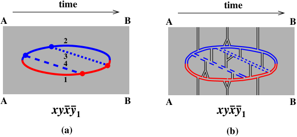
Figure 23: One of the two distinct large-$N_{\rm c}$ color routings of the $xy\bar{x}\bar{y}$ interference diagram drawn on a cylinder. The top edge AB of the shaded region is to be identified with the bottom edge AB. (b) explicitly shows the corresponding color flow for an example of medium background field correlations (black) that gives a planar diagram (and so leading-order in $1/N_{\rm c}$). In our notation, this interference contribution could be referred to as either $xy\bar{x}\bar{y}_{1}$ or $xz\bar{x}\bar{z}_{2}$.

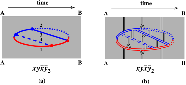
Figure 24: As fig. 23 but showing the other distinct color routing of $xy\bar{x}\bar{y}$. In our notation, this interference contribution could be referred to as either $xy\bar{x}\bar{y}_{2}$ or $xz\bar{x}\bar{z}_{1}$.

The distinguishing difference between the calculations of the two color routings will, in the language of the preceding paper 2brem , be the assignments of the longitudinal momentum fractions $x_{i}$ for the 4-particle part of the evolution $t_{\rm y}<t<t_{\bar{\rm x}}$. Going around the cylinder, the first routing $xy\bar{x}\bar{y}_{1}$ has (as labeled in fig. 23)

$$(x_{1},x_{2},x_{3},x_{4})=(-1,1{-}x{-}y,y,x),$$ (43)

whereas the second routing $xy\bar{x}\bar{y}_{2}$ has (as labeled in fig. 24),

$$(x_{1},x_{2},x_{3},x_{4})=(-1,y,1{-}x{-}y,x)\equiv(\hat{x}_{1},\hat{x}_{2},\hat{x}_{3},\hat{x}_{4}).$$ (44)

Because this last assignment is identical to the one used for the canonical diagram analyzed in ref. 2brem , we will focus on the evaluation of $xy\bar{x}\bar{y}_{2}$ to simplify comparison with previous work. Then, if we define

$$\Psi(x,y,z)\equiv 2\operatorname{Re}\left[\Delta\frac{d\Gamma}{dx\,dy}\right]_{xy\bar{x}\bar{y}_{2}},$$ (45)

the full result that we want from $xy\bar{x}\bar{y}$ plus its distinct permutations, including all distinct color routings, is

$$\Psi(x,y,z)+\Psi(y,z,x)+\Psi(z,x,y)+\Psi(y,x,z)+\Psi(x,z,y)+\Psi(z,y,x).$$ (46)

We mention in passing that the reason we could sidestep discussion of color routings for the $x\bar{x}y\bar{y}$ diagram analyzed in section II.1 is because in that case there was no interval of 4-particle evolution and so no distinction like (43) vs. (44). Unlike 4-particle evolution, the choice of ordering of the $x_{i}$ for 3-particle evolution makes no difference to the calculation since 3 high-energy particles are all neighbors when drawn on our time-ordered cylinder.

II.2.2 Result and small-$\Delta t$ behavior

In notation similar to that used in the preceding paper 2brem , the final result for $xy\bar{x}\bar{y}_{2}$ is

$$\left[\frac{d\Gamma}{dx\,dy}\right]_{xy\bar{x}\bar{y}_{2}}=\int_{0}^{\infty} d(\Delta t)\>\frac{C_{\rm A}^{2}\alpha_{\rm s}^{2}M_{\rm i}M_{\rm f}^{\rm seq}}{32\pi^{4}E^{2}}\,({-}\hat{x}_{1}\hat{x}_{2}\hat{x}_{3}\hat{x}_{4})\Omega_{+}\Omega_{-}\csc(\Omega_{+}\Delta t)\csc(\Omega_{-}\Delta t)$$

$$\times\Bigl{\{}(\bar{\beta}Y_{\rm y}^{\rm seq}Y_{\bar{\rm x}}^{\rm seq}+\bar{\alpha}\overline{Y}_{{\rm y}{\bar{\rm x}}}^{\,{\rm seq}}Y_{{\rm y}{\bar{\rm x}}}^{\rm seq})I_{0}^{\rm seq}+(\bar{\alpha}+\bar{\beta}+2\bar{\gamma})Z_{{\rm y}{\bar{\rm x}}}^{\rm seq}I_{1}^{\rm seq}$$

$$\quad+\bigl{[}(\bar{\alpha}+\bar{\gamma})Y_{\rm y}^{\rm seq}Y_{\bar{\rm x}}^{\rm seq}+(\bar{\beta}+\bar{\gamma})\overline{Y}_{{\rm y}{\bar{\rm x}}}^{\,{\rm seq}}Y_{{\rm y}{\bar{\rm x}}}^{\rm seq}\bigr{]}I_{2}^{\rm seq}$$

$$\quad-(\bar{\alpha}+\bar{\beta}+\bar{\gamma})(\overline{Y}_{{\rm y}{\bar{\rm x}}}^{\,{\rm seq}}Y_{\bar{\rm x}}^{\rm seq}I_{3}^{\rm seq}+Y_{\rm y}^{\rm seq}Y_{{\rm y}{\bar{\rm x}}}^{\rm seq}I_{4}^{\rm seq})\Bigl{\}}$$ (47)

where formulas for the various symbols are given in appendix E and $\Delta t$ represents the intermediate time interval $t_{\bar{\rm x}}-t_{\rm y}$. This formula is identical to that for $xy\bar{y}\bar{x}$ in ref. 2brem except for the addition of a superscript “seq” on some symbols (standing for “sequential” interference diagram as opposed to crossed), the bars on $(\bar{\alpha},\bar{\beta},\bar{\gamma})$, and subscript labels $\bar{y}$ there replaced by $\bar{x}$ here. These modifications are explained in the appendix.

The small $\Delta t$ limit of the integrand is also discussed in the appendix, with result

$$\left[\frac{d\Gamma}{dx\,dy}\right]_{xy\bar{x}\bar{y}_{2}} =\frac{\alpha_{\rm s}^{2}\,P(x)\,P({\mathfrak{y}})}{8\pi^{2}(1-x)}\,\int_{0}d(\Delta t)\left(\frac{1}{(\Delta t)^{2}}-\frac{i(\Omega_{E,x}+\Omega_{(1-x)E,{\mathfrak{y}}})}{\Delta t}\right)$$

$$\quad\qquad+{\rm UV~{}convergent}.$$ (48)

As in ref. 2brem , the $1/(\Delta t)^{2}$ divergence may be eliminated by subtracting out the vacuum calculation (which must total to zero when summed over all interference processes). If we now add in the conjugate diagram $\bar{x}\bar{y}xy_{2}$, that leaves

$$2\operatorname{Re}\left[\frac{d\Gamma}{dx\,dy}\right]_{xy\bar{x}\bar{y}_{2}} \to-\frac{\alpha_{\rm s}^{2}\,P(x)\,P({\mathfrak{y}})}{4\pi^{2}(1-x)}\,\operatorname{Re}\Bigl{[}(i\Omega_{E,x}+i\Omega_{(1-x)E,{\mathfrak{y}}})\int_{0}\frac{d(\Delta t)}{\Delta t}\Bigr{]}$$

$$\quad\qquad+{\rm UV~{}convergent}.$$ (49)

This result is invariant under $y\leftrightarrow z$ and so will be the same for the other color routing $xy\bar{x}\bar{y}_{1}$. In total, then

$$2\operatorname{Re}\left[\frac{d\Gamma}{dx\,dy}\right]_{xy\bar{x}\bar{y}} \to-\frac{\alpha_{\rm s}^{2}\,P(x)\,P({\mathfrak{y}})}{2\pi^{2}(1-x)}\,\operatorname{Re}\Bigl{[}(i\Omega_{E,x}+i\Omega_{(1-x)E,{\mathfrak{y}}})\int_{0}\frac{d(\Delta t)}{\Delta t}\Bigr{]}$$

$$\quad\qquad+{\rm UV~{}convergent}.$$ (50)

For real $\Delta t$, this indeed cancels the small-$\Delta t$ behavior of (39), as promised. So our final $\Delta t$ integrals for the sum of all sequential diagrams (fig. 13) will be convergent.

II.3 Pole Contributions

As mentioned earlier and as discussed in the previous paper 2brem , one needs to be careful about the cancellation of $1/\Delta t$ divergences between different diagrams, such as for the sum of (39) and (50) in the present case. The problem is that there can be contributions coming from the pole at $\Delta t{=}0$ that need to be accounted for. The previous paper 2brem attempted to isolate these pole contributions by appropriate replacements of the form

$$\int_{0}^{\infty}\frac{d(\Delta t)}{\Delta t}\,\cdots~{}\to~{}\int_{0}^{\infty}\frac{d(\Delta t)}{\Delta t\pm i\epsilon}\,\cdots$$ (51)

for each $\Delta t$ integral. The same method applied to the sequential diagrams would give a pole contribution to $\Phi+\Psi\equiv\frac{1}{2}[2\operatorname{Re}(x\bar{x}y\bar{y}+x\bar{x}\bar{y}y)-{\rm IMC}]+2\operatorname{Re}(xy\bar{x}\bar{y}_{2})$ of

$$\frac{\alpha_{\rm s}^{2}\,P(x)\,P({\mathfrak{y}})}{8\pi(1-x)}\,\operatorname{Re}(\Omega_{E,x}+\Omega_{(1-x)E,{\mathfrak{y}}}).$$ (52)

We will refer to this as a “$1/\pi$” contribution because of the single factor of $\pi$ in the denominator. It turns out that both this result for the pole contribution to the sequential diagrams and the previous result 2brem for the pole contribution to the crossed diagrams are incomplete: They miss some additional terms that involve $1/\pi^{2}$. The proper calculation of the pole terms is a lengthy enough issue that it would distract from our focus in this paper, and so here we will just quote results. The full discussion of why the previous analysis was incomplete, and of how to compute the full pole pieces (using dimensional regularization), is left to ref. dimreg .

With regard to sequential diagrams, the result is that (52) should be supplemented by the additional contribution

$$-\frac{\alpha_{\rm s}^{2}\,P(x)\,P({\mathfrak{y}})}{4\pi^{2}(1-x)}\operatorname{Re}(i\Omega_{E,x}+i\Omega_{(1-x)E,{\mathfrak{y}}}).$$ (53)

For crossed diagrams, which are also needed for our total results of figs. 16 and 17, the corrected pole contribution will be given in section III.2 below. This correction is, in fact, critical to the Gunion-Bertsch-like cancellation of logarithms (10) discussed in Appendix B.

III Summary of Formula

III.1 Sequential Diagrams

We now give a summary of our final formulas for the sequential diagrams of fig. 13, in the same style as the summary of the crossed-diagram contribution in section VIII of the preceding paper 2brem . The two should be added together (along with the contributions involving 4-gluon vertices, like fig. 14, which we have left for the future).

The main result of this paper is

$$\left[\Delta\frac{d\Gamma}{dx\>dy}\right]_{\rm sequential}=\quad {\cal A}_{\rm seq}(x,y)+{\cal A}_{\rm seq}(1{-}x{-}y,y)+{\cal A}_{\rm seq}(x,1{-}x{-}y)$$

$$+~{} {\cal A}_{\rm seq}(y,x)+{\cal A}_{\rm seq}(y,1{-}x{-}y)+{\cal A}_{\rm seq}(1{-}x{-}y,x)$$ (54)

where ${\cal A}_{\rm seq}(x,y)$ is the result for (i) $2\operatorname{Re}(xy\bar{x}\bar{y}_{2})$, for the large-$N_{\rm c}$ color routing of fig. 24, plus half of (ii) $2\operatorname{Re}(x\bar{x}y\bar{y}+x\bar{x}\bar{y}y)$ minus the corresponding idealized Monte Carlo result. That is, ${\cal A}_{\rm seq}$ corresponds to $\Psi+\Phi$ in the notation of (42) and (46). We will write this as

$${\cal A}_{\rm seq}(x,y)={\cal A}^{\rm pole}_{\rm seq}(x,y)+\int_{0}^{\infty}d(\Delta t)\>\Bigl{[}2\operatorname{Re}\bigl{(}B_{\rm seq}(x,y,\Delta t)\bigr{)}+F_{\rm seq}(x,y,\Delta t)\bigr{]},$$ (55)

where

$$B_{\rm seq}(x,y,\Delta t) =C_{\rm seq}(\{\hat{x}_{i}\},\bar{\alpha},\bar{\beta},\bar{\gamma},\Delta t)$$

$$=C_{\rm seq}({-}1,y,1{-}x{-}y,x,\bar{\alpha},\bar{\beta},\bar{\gamma},\Delta t)$$ (56)

corresponds to $xy\bar{x}\bar{y}_{2}$. The other term, $F_{\rm seq}$, corresponds to half of $2\operatorname{Re}(x\bar{x}y\bar{y}+x\bar{x}\bar{y}y)$ minus the corresponding idealized Monte Carlo result. $C$ is defined to have the vacuum result subtracted, so write

$$C_{\rm seq}=D_{\rm seq}-\lim_{\hat{q}\to 0}D_{\rm seq}.$$ (57)

$D_{\rm seq}$, defined as the integrand for $xy\bar{x}\bar{y}_{2}$, is given by

$$D_{\rm seq}(x_{1}, x_{2},x_{3},x_{4},\bar{\alpha},\bar{\beta},\bar{\gamma},\Delta t)=$$

$$\frac{C_{\rm A}^{2}\alpha_{\rm s}^{2}M_{\rm i}M_{\rm f}^{\rm seq}}{32\pi^{4}E^{2}}\,({-}x_{1}x_{2}x_{3}x_{4})\Omega_{+}\Omega_{-}\csc(\Omega_{+}\Delta t)\csc(\Omega_{-}\Delta t)$$

$$\times\Bigl{\{}(\bar{\beta}Y_{\rm y}^{\rm seq}Y_{\bar{\rm x}}^{\rm seq}+\bar{\alpha}\overline{Y}_{{\rm y}{\bar{\rm x}}}^{\,{\rm seq}}Y_{{\rm y}{\bar{\rm x}}}^{\rm seq})I_{0}^{\rm seq}+(\bar{\alpha}+\bar{\beta}+2\bar{\gamma})Z_{{\rm y}{\bar{\rm x}}}^{\rm seq}I_{1}^{\rm seq}$$

$$\quad+\bigl{[}(\bar{\alpha}+\bar{\gamma})Y_{\rm y}^{\rm seq}Y_{\bar{\rm x}}^{\rm seq}+(\bar{\beta}+\bar{\gamma})\overline{Y}_{{\rm y}{\bar{\rm x}}}^{\,{\rm seq}}Y_{{\rm y}{\bar{\rm x}}}^{\rm seq}\bigr{]}I_{2}^{\rm seq}$$

$$\quad-(\bar{\alpha}+\bar{\beta}+\bar{\gamma})(\overline{Y}_{{\rm y}{\bar{\rm x}}}^{\,{\rm seq}}Y_{\bar{\rm x}}^{\rm seq}I_{3}^{\rm seq}+Y_{\rm y}^{\rm seq}Y_{{\rm y}{\bar{\rm x}}}^{\rm seq}I_{4}^{\rm seq})\Bigl{\}}.$$ (58)

$(\bar{\alpha},\bar{\beta},\bar{\gamma})$, the $(X^{\rm seq},Y^{\rm seq},Z^{\rm seq})$ and the $I^{\rm seq}$ are given in appendix E by (117), (125), and (126) respectively. The 4-particle evolution frequencies $\Omega_{\pm}$ are given by eq. (5.21) of ref. 2brem . The $M$ and other $\Omega$ here are

$$M_{\rm i}=x_{1}x_{4}(x_{1}{+}x_{4})E,\qquad M_{\rm f}^{\rm seq}=x_{2}x_{3}(x_{2}{+}x_{3})E$$ (59)

and

$$\Omega_{\rm i}=\sqrt{-\frac{i\hat{q}_{\rm A}}{2E}\left(\frac{1}{x_{1}}+\frac{1}{x_{4}}-\frac{1}{x_{1}{+}x_{4}}\right)},\qquad\Omega_{\rm f}^{\rm seq}=\sqrt{-\frac{i\hat{q}_{\rm A}}{2E}\left(\frac{1}{x_{2}}+\frac{1}{x_{3}}-\frac{1}{x_{2}+x_{3}}\right)}$$ (60)

[which equal $\Omega_{E,x}$ (36) and $\Omega_{(1-x)E,{\mathfrak{y}}}$ (38) when $\{x_{i}\}=\{\hat{x}_{i}\}$]. Next,

$$F_{\rm seq}(x,y,\Delta t)=\frac{\alpha_{\rm s}^{2}P(x)P(\frac{y}{1-x})}{4\pi^{2}(1-x)}\Bigl{[} \operatorname{Re}(i\Omega_{\rm i})\,\operatorname{Re}\bigl{(}\Delta t\,(\Omega_{\rm f}^{\rm seq})^{2}\csc^{2}(\Omega_{\rm f}^{\rm seq}\,\Delta t)\bigr{)}$$

$$+ \operatorname{Re}(i\Omega_{\rm f}^{\rm seq})\,\operatorname{Re}\bigl{(}\Delta t\,\Omega_{\rm i}^{2}\csc^{2}(\Omega_{\rm i}\,\Delta t)\bigr{)}\Bigr{]}.$$ (61)

Finally, the pole piece is

$${\cal A}_{\rm seq}^{\rm pole}(x,y)=\frac{\alpha_{\rm s}^{2}\,P(x)\,P({\mathfrak{y}})}{2\pi^{2}(1-x)}\biggl{(}-\tfrac{1}{2}\operatorname{Re}(i\Omega_{E,x}+i\Omega_{(1-x)E,{\mathfrak{y}}})+\tfrac{\pi}{4}\operatorname{Re}(\Omega_{E,x}+\Omega_{(1-x)E,{\mathfrak{y}}})\biggr{)}.$$ (62)

In the last formulas, $P(x)$ refers to the spin-averaged $g{\to}gg$ DGLAP splitting function

$$P_{g\to gg}(x)=C_{\rm A}\,\frac{[1+x^{4}+(1{-}x)^{4}]}{x(1{-}x)}\,.$$ (63)

III.2 Crossed Diagrams

The formulas for crossed diagrams are summarized in section VIII of ref. 2brem , except that the pole contribution there needs to be corrected dimreg by replacing the term

$$2\operatorname{Re}\left[\frac{d\Gamma}{dx\,dy}\right]_{\rm fig.~{}23}^{\rm pole}$$ (64)

in the formula (8.2) for $A(x,y)$ in ref. 2brem by

$$A^{\rm pole}(x,y) \equiv 2\operatorname{Re}\Biggl{[}\frac{C_{\rm A}^{2}\alpha_{\rm s}^{2}}{16\pi^{2}}\,xy(1{-}x)^{2}(1{-}y)^{2}(1{-}x{-}y)^{2}$$

$$\qquad~{}\times\biggl{\{}-i[\Omega_{-1,1-x,x}+\Omega_{-(1-y),1-x-y,x}-\Omega_{-1,1-y,y}^{*}-\Omega_{-(1-x),1-x-y,y}^{*}]$$

$$\qquad~{}\qquad\times\biggl{[}\left((\alpha+\beta)+\frac{(\alpha+\gamma)xy}{(1{-}x)(1{-}y)}\right)\ln\left(\frac{1{-}x{-}y}{(1{-}x)(1{-}y)}\right)+\frac{2(\alpha+\beta+\gamma)xy}{(1{-}x)(1{-}y)}\biggr{]}$$

$$\qquad~{}\quad-\pi[\Omega_{-1,1-x,x}+\Omega_{-(1-y),1-x-y,x}+\Omega_{-1,1-y,y}^{*}+\Omega_{-(1-x),1-x-y,y}^{*}]$$

$$\qquad~{}\qquad\times\left((\alpha+\beta)+\frac{(\alpha+\gamma)xy}{(1{-}x)(1{-}y)}\right)\biggr{\}}\Biggr{]}.$$ (65)

The $\pi/\pi^{2}$ terms above are the same as in ref. 2brem but are corrected by the addition of the $1/\pi^{2}$ terms also included above.

IV Conclusion

We have still not computed contributions from 4-gluon vertices such as fig. 14, which we expect will be important when no final gluon is soft, i.e. when $y\sim x\sim z$. (Conversely, we believe that these contributions will not be important when at least one final gluon is soft.) To use our results for energy loss calculations, we will also need to consider virtual corrections to single gluon bremsstrahlung. Both of these calculations have been left for future work.

One of the interesting aspects of our results in fig. 17 is the sign of the correction $\Delta\,d\Gamma/dx\,dy$ due to overlapping formation times. We finish below with a qualitative picture of why the correction should be negative for $y\ll x,z$. Unfortunately, we do not have any simple, compelling, qualitative argument for the other, more important case: How can we simply understand why the correction should be positive for $y\sim x\ll z$ (and possibly also for $y\sim x\sim z$, depending on the size and sign of 4-gluon vertex contributions)?

A picture of why $\Delta\,d\Gamma/dx\,dy$ is negative for $y\ll x,z$

Consider $y\ll x<z$. As reviewed earlier, QCD formation times for softer emissions are smaller than formation times for harder emissions; so the formation time for emitting $y$ is small compared to the formation time for emitting $x$. Now consider the case where these formation times overlap, as shown in fig. 25a. We’ve chosen to look at a case where the $y$ emission happens some time $\delta$ after the midpoint of the $x$ emission. The analogous contribution in the idealized Monte Carlo calculation is shown in fig. 25b. In the idealized Monte Carlo calculation, which ignores formation times, we have treated the “time” of the $x$ and $y$ emissions to be the midpoints of the corresponding formation times in fig. 25a. (This is the natural choice. Remember that it is also the choice we used in section II.1.2 and technically justify in appendix D.)

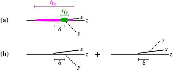
Figure 25: (a) A double-bremsstrahlung process with $y\ll x$ and overlapping formation times. $t_{\rm fx}$ and $t_{\rm fy}$ indicate the scale of the formation times for $x$ and $y$ emission respectively. (b) The corresponding idealized Monte Carlo contributions. $\delta$ is the time separation between the $x$ emission and the $y$ emission, defined in (a) as the separation between the midpoint times $\tau_{x}$ and $\tau_{y}$ of (26). As usual, transverse separations are highly exaggerated in the drawing. [There is no significance to (i) $y$ being drawn angled up rather than down in the last term or (ii) the slightly exaggerated transverse separation of $x$ in the drawing of (b) compared to (a). Both were done just to make the diagram clearer and less crowded.]

In the idealized Monte Carlo calculation, the chance of $y$ emission from the $x$ daughter is treated as completely independent from the chance of $y$ emission from the $z$ daughter, and these two probabilities are added together. But the separation of the $x$ and $z$ daughters is actually so small on these time scales that the $y$ emission cannot resolve them as distinct particles when $y\ll x$.

Specifically, $x$ emission is associated with transverse momenta of order $Q_{\perp,x}\sim\sqrt{\hat{q}t_{\rm form,x}}$. Using the formation time (3), the corresponding scale of transverse separation of $x$ from $z$ during that formation time is $b_{x}\sim 1/Q_{\perp,x}\sim(xE\hat{q})^{-1/4}$. When $y\ll x$, this is indeed very small compared to the similar transverse scale characterizing the $y$ emission during its formation time: $b_{y}\sim(yE\hat{q})^{-1/4}$.

So, instead of seeing two daughter gluons ($x$ and $z$), the $y$ emission effectively sees a single adjoint-charge particle. (This resolution issue is similar to work by Mehtar-Tani, Salgado, and Konrad resolution .) On these time scales, there is therefore effectively only one particle providing a chance for initiating $y$ emission rather than the two particles in the idealized Monte Carlo calculation associated with fig. 25b. That is, idealized Monte Carlo overcounts the probability for the $y$ emission, and so the correction to idealized Monte Carlo should be negative for $y\ll x$.

Appendix A Approximate analytic formula fitted to result

The following approximation reproduces the results of fig. 17 with a maximum absolute error of 0.017 for all $y>10^{-4}$ (assuming one permutes the final state gluons to choose $y<x<z$, just as in fig. 17):

$$\pi^{2}\,x\,y^{\frac{3}{2}}\,\Delta\,\frac{d\Gamma}{dxdy}=\sum^{3}_{m=0}\sum^{4}_{n=0}\left(a_{mn}+b_{mn}\Big{(}\frac{y}{x}\Big{)}^{\frac{1}{3}}\right)s^{m}t^{n},$$ (66)

where the parameters

$$s\equiv\frac{2(x-y)}{t},\qquad t\equiv 2x+y$$ (67)

each vary independently from 0 to 1. The numerical coefficients $a_{mn}$ and $b_{mn}$ are given in tables 1 and 2. We have made no effort to make the approximation work well for $y<10^{-4}$.

	0	1	2	3	4
0	-4.98232	40.5485	-198.390	351.600	-202.365
1	6.33241	-81.4351	409.898	-730.480	419.607
2	-2.31929	49.1060	-251.070	448.653	-257.366
3	0.0211282	-7.27248	38.4361	-68.9343	39.6011

Table 1: The coefficients $a_{mn}$ in eq. (66).

	0	1	2	3	4
0	5.46263	-40.7646	199.438	-353.153	203.648
1	-3.79756	61.5337	-312.829	558.682	-321.248
2	0.227523	-19.0923	100.471	-180.559	103.988
3	0.399152	-3.44293	16.6646	-29.2812	16.5223

Table 2: The coefficients $b_{mn}$ in eq. (66).

Appendix B Logarithms and their cancellation

In this appendix, we discuss the behavior of individual contributions to $\Delta\,d\Gamma/dx\,dy$ in the $y\ll x\ll 1$ limit. The individual contributions are logarithmically enhanced compared to the total, as in (10). In more detail,

$$\left[\frac{d\Gamma}{dx\,dy}\right]_{\rm crossed} \approx-\frac{3}{2}\,\frac{C_{\rm A}^{2}\alpha_{\rm s}^{2}}{\pi^{2}xy^{3/2}}\sqrt{\frac{\hat{q}}{E}}\,\ln\left(\frac{x}{y}\right),$$ (68a)

$$\left[\Delta\frac{d\Gamma}{dx\,dy}\right]_{\rm seq\phantom{ssed}} \approx+\frac{3}{2}\,\frac{C_{\rm A}^{2}\alpha_{\rm s}^{2}}{\pi^{2}xy^{3/2}}\sqrt{\frac{\hat{q}}{E}}\,\ln\left(\frac{x}{y}\right),$$ (68b)

where $\approx$ indicates that we are only showing the leading logarithm. We can break the contributions down somewhat further, as shown in Table 3. (One way to extract the coefficients in this table is from numerical extrapolation, as shown in fig. 26.)

$2\operatorname{Re}(xy\bar{y}\bar{x}+x\bar{y}y\bar{x})$	$A(x,y)$	$-\tfrac{1}{2}$
$2\operatorname{Re}(zy\bar{y}\bar{z}+z\bar{y}y\bar{z})$	$A(z,y)$	$-\tfrac{1}{2}$
$2\operatorname{Re}(x\bar{z}z\bar{x}+x\bar{z}\bar{x}z+z\bar{x}x\bar{z}+z\bar{x}\bar{z}x)$	$A(x,z)$	$-\tfrac{1}{2}$
$2\operatorname{Re}(x\bar{x}y\bar{y}+x\bar{x}\bar{y}y)-{\rm IMC}$	${\cal A}_{\rm seq}(x,y)+{\cal A}_{\rm seq}(x,z)$	$+\tfrac{1}{2}$
$2\operatorname{Re}(z\bar{z}y\bar{y}+z\bar{z}\bar{y}y)-{\rm IMC}$	${\cal A}_{\rm seq}(z,y)+{\cal A}_{\rm seq}(z,x)$	$+\tfrac{1}{2}$
$2\operatorname{Re}(y\bar{y}x\bar{x}+y\bar{y}\bar{x}x)-{\rm IMC}$	${\cal A}_{\rm seq}(y,x)+{\cal A}_{\rm seq}(y,z)$	$+\tfrac{1}{2}$

Table 3: Coefficients of logarithms. The first column lists the subset of diagrams that are responsible for generating logarithms, using the notation of figs. 10–13 (to include permutations of $x$, $y$, and $z$). The second column identifies the UV-safe combinations that contain those diagrams, with ${\cal A}_{\rm seq}$ given by (55) of this paper. $A$ is given by eq. (8.2) of ref. 2brem , as corrected by section III.2 of this paper. The last column is the corresponding leading-log contribution to $\Delta\,d\Gamma/dx\,dy$ in units of $\frac{C_{\rm A}^{2}\alpha_{\rm s}^{2}}{\pi^{2}xy^{3/2}}\bigl{(}\frac{\hat{q}}{E}\bigr{)}^{1/2}\,\ln\bigl{(}\frac{x}{y}\bigr{)}$.

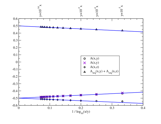
Figure 26: Various pieces of $\Delta\,d\Gamma/dx\,dy$ (corresponding to Table 3), in units of $\frac{C_{\rm A}^{2}\alpha_{\rm s}^{2}}{\pi^{2}xy^{3/2}}\bigl{(}\frac{\hat{q}}{E}\bigr{)}^{1/2}\,\ln\bigl{(}\frac{x}{y}\bigr{)}$. The results are plotted against $1/\log_{10}(x/y)$, which allows for a simple linear extrapolation of the $y\to 0$ limit for fixed $x$. Data points were calculated for $x=10^{-3}$, and we checked that results for $x=10^{-4}$ would be indistinguishable to the eye. Note that the $\times$ and $\circ$ data points are hard to distinguish because they are almost on top of each other. We have not shown points for ${\cal A}_{\rm seq}(y,x)+{\cal A}_{\rm seq}(y,z)$ and ${\cal A}_{\rm seq}(z,y)+{\cal A}_{\rm seq}(z,x)$: these would both lie right on top of the ${\cal A}_{\rm seq}(x,y)+{\cal A}_{\rm seq}(x,z)$ points.

B.1 DGLAP

There is a relatively simple way to understand some of these logarithms. Let’s consider the $2\operatorname{Re}(x\bar{x}y\bar{y}+x\bar{x}\bar{y}y)$ entry of Table 3, which corresponds to the second and third diagrams of figs. 12 and 13. Since $y$ is the softest high-energy particle in the process, it is the one most affected by the medium (which is, recall, why its formation time is the shortest). So focus attention on the contributions to this process where the only interaction with the medium occurs during the $y$ emission. That is, consider fig. 27. In this picture, the $x$ emission looks like an initial-state radiation correction to the underlying process of the $y$ emission. Initial-state radiation generates a factorizable logarithm associated with DGLAP evolution. Let’s calculate it. For the sake of familiarity, we’ll start from the usual leading-order DGLAP evolution equation (though that is a somewhat backwards way to start given how DGLAP evolution is derived in the first place).

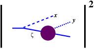
Figure 27: Magnitude squared of a Feynman diagram, representing $2\operatorname{Re}(x\bar{x}y\bar{y}+x\bar{x}\bar{y}y)$ if interactions with the medium are only considered for the $y$ emission. The blob represents those medium interactions, and everything preceding the blob is approximated as effectively in vacuum.

Consider the (vacuum) DGLAP evolution of an initial parton distribution function $f(\zeta,Q^{2})$ for a parton of energy $\zeta E$. (We use the symbol $\zeta$ for momentum fraction here instead of the more traditional $x$ or $z$ just to avoid confusion with the specific use of $x$, $y$, and $z\equiv 1{-}x{-}y$ in this paper as the momentum fractions of the three final-state gluons.) The basic DGLAP evolution equation takes the form

$$\frac{df(\zeta,Q^{2})}{d\ln(Q^{2})}=\frac{\alpha_{\rm s}}{2\pi}\int_{\zeta}^{1}\frac{d\xi}{\xi}\>P(\xi)\,f\bigl{(}\frac{\zeta}{\xi},Q^{2}\bigr{)},$$ (69)

where $P$ is the relevant DGLAP splitting function. Now formally solve perturbatively by iteration, writing $f=f_{0}+f_{1}+\cdots$ with $f_{0}(\zeta)=\delta(1-\zeta)$ representing the case of no initial radiation. Then $f_{1}$ (corresponding to a single DGLAP emission from the initial state) is given by

$$\frac{df_{1}(\zeta,Q^{2})}{d\ln(Q^{2})}=\frac{\alpha_{\rm s}}{2\pi}\int_{\zeta}^{1}\frac{d\xi}{\xi}\>P(\xi)\,f_{0}\bigl{(}\frac{\zeta}{\xi},Q^{2}\bigr{)}=\frac{\alpha_{\rm s}}{2\pi}\,P(\zeta).$$ (70)

The solution is

$$f_{1}(\zeta,Q^{2})=\frac{\alpha_{\rm s}}{2\pi}\,P(\zeta)\,\ln\frac{Q^{2}}{Q_{0}^{2}}\,,$$ (71)

where we’ll discuss what the reference momentum $Q_{0}^{2}$ should be in a moment. The result we want combines this probabilistic description of the initial $x$ emission with the rate for the sub-process associated with the blob in fig. 27. That sub-process represents the rate of $y$ emission in the medium, and so the leading-log estimate of the contribution to $d\Gamma/dx\,dy$ associated with fig. 27 should be

$$\left[\frac{d\Gamma}{dx\,dy}\right]_{{\rm initial}~{}x}\approx f_{1}(1{-}x,Q^{2})\,\frac{d\Gamma}{dy}=\frac{\alpha_{\rm s}}{2\pi}\,P(1{-}x)\,\ln\Bigl{(}\frac{Q^{2}}{Q_{0}^{2}}\Bigr{)}\,\frac{d\Gamma}{dy}.$$ (72)

In the main text and in the preceding paper 2brem , our convention has usually been to identify the argument of the DGLAP splitting function with the momentum fraction $x$ of the emitted gluon instead of with $\zeta=1{-}x$ in fig. 27. Since the relevant splitting $g\to gg$ for this paper is symmetric, it doesn’t matter in any case. So we’ll henceforth rewrite $P(1{-}x)$ above as $P(x)$.

The remaining job is to figure out the scales of the relevant upper and lower kinematic bounds on DGLAP virtuality $Q^{2}$ as applies to our problem, in order to know what ratio appears in the logarithm in (72). In the high-energy, nearly-collinear limit, virtuality is related to off-shellness $\Delta E$ of energy by $Q^{2}\sim E_{Q}\,\Delta E$. In the case of fig. 27, $E_{Q}\simeq E$ for small $x$, where $E$ is the initial parton energy. $\Delta E$ is related to time by the uncertainty principle, and so $Q^{2}\sim E/\Delta t_{x}$, where $\Delta t_{x}$ is the time scale associated with the $x$ emission. So, (72) can be translated to

$$\left[\frac{d\Gamma}{dx\,dy}\right]_{{\rm initial}~{}x}\approx\frac{\alpha_{\rm s}}{2\pi}\,P(x)\,\ln\Bigl{(}\frac{\Delta t_{x}^{\rm max}}{\Delta t_{x}^{\rm min}}\Bigr{)}\,\frac{d\Gamma}{dy}.$$ (73)

The time scale $\Delta t_{y}$ of the underlying $y$ emission is the formation time $t_{{\rm form},y}$, which provides the lower limit on the time scale $\Delta t_{x}$ for generating a DGLAP logarithm.

In the above DGLAP analysis based on fig. 27, we assumed that medium effects on the $x$ emission could be ignored. This assumption is only valid for time scale small compared to the formation time $t_{{\rm form},x}$ for $x$ emission. Another way to explain this infrared cut-off is to note that the logarithm in (72) is a collinear logarithm. In vacuum, the $x$ and $\zeta$ particle trajectories can be arbitrarily collinear, and there is no small-angle cut-off for collinear logarithms if we ignore the masses of particles. In medium, however, particles constantly change their direction over time, and so the $x$ and $\zeta$ trajectories cannot remain collinear over arbitrarily large times. Formation times tell you how long you can wait before such changes destroy quantum coherence. The upshot is that the relevant range of $\Delta t$ for which a vacuum DGLAP analysis applies is

$$t_{{\rm form},y}\lesssim\Delta t_{x}\lesssim t_{{\rm form},x}.$$ (74)

Correspondingly the logarithm in (72) is $\ln(t_{{\rm form},x}/t_{{\rm form},y})$. Combining $t_{{\rm form},x}\propto\sqrt{x}$ from (3) with the soft limits $P(x)\simeq 2C_{\rm A}/x$ from (63) and

$$\frac{d\Gamma}{dy}\simeq\frac{C_{\rm A}\alpha_{\rm s}}{\pi y^{3/2}}\sqrt{\frac{\hat{q}_{\rm A}}{E}}$$ (75)

from (35) and (36) then gives

$$\left[\frac{d\Gamma}{dx\,dy}\right]_{{\rm initial}~{}x}\approx\frac{C_{\rm A}^{2}\alpha_{\rm s}^{2}}{2\pi^{2}xy^{3/2}}\,\ln\Bigl{(}\frac{x}{y}\Bigr{)}.$$ (76)

As promised, this agrees with the $2\operatorname{Re}(x\bar{x}y\bar{y}+x\bar{x}\bar{y}y)$ entry of Table 3.

Readers may wonder why, in our discussion above (and especially in our discussion of Gunion-Bertsch cancellation below), we have focused on (i) vacuum $x$ radiation from an underlying medium-induced soft $y$-emission process, rather than (ii) soft, vacuum $y$ radiation from an underlying medium-induced $x$-emission process. The reason is that the latter contribution to real double bremsstrahlung $d\Gamma/dx\,dy$ is sub-leading compared to the former by a factor of $\sqrt{y/x}$. To understand this, consider the $x{\leftrightarrow}y$ analog of (73), which would contribute to $d\Gamma/dx\,dy$ something of order $\alpha_{\rm s}\,P(y)\,\frac{d\Gamma}{dx}\times\log$. Since $d\Gamma/dx\sim\alpha_{\rm s}/x^{3/2}$ in units of $\sqrt{\hat{q}/E}$, this gives a contribution to $d\Gamma/dx\,dy$ of order $(\alpha_{\rm s}^{2}/x^{3/2}y)\times\log$, which is sub-leading compared to (68) and (9).

B.2 Gunion-Bertsch

If we carry further the model we used in drawing fig. 27, we might expect the logarithmic corrections to the total rate to be similarly related to fig. 28. If we now abstract the $y$ emission process and its attendant medium interaction as a net injection of momentum, then Fig. 28 looks perhaps analogous to the process of fig. 29. The latter figure shows the type of non-Abelian radiation process long ago considered by Gunion and Bertsch GB in the context of 2-particle collisions in vacuum. In the high-energy, nearly-collinear limit, the amplitude takes the form

$$-gT^{b}T^{a}\frac{{\bm{k}}_{\perp}\cdot{\bm{\varepsilon}}_{\perp}(1-x)}{{\bm{k}}_{\perp}^{2}}+gT^{a}T^{b}\,\frac{({\bm{k}}_{\perp}-x{\bm{l}}_{\perp})\cdot{\bm{\varepsilon}}_{\perp}(1-x)}{|{\bm{k}}_{\perp}-x{\bm{l}}_{\perp}|^{2}}-g[T^{a},T^{b}]\,\frac{({\bm{k}}_{\perp}-{\bm{l}}_{\perp})\cdot{\bm{\varepsilon}}_{\perp}(1-x)}{|{\bm{k}}_{\perp}-{\bm{l}}_{\perp}|^{2}},$$ (77)

where $\perp$ is defined relative to the initial particle direction, ${\bm{l}}_{\perp}$ and $a$ characterize the transverse momentum transfer and adjoint color index associated with the collision, and ${\bm{k}}_{\perp}$ and $b$ characterize the transverse momentum and adjoint color index of the final bremsstrahlung gluon. In the $k_{\perp}\gg l_{\perp}$ limit, if we keep only the leading behavior of each individual diagram, the corresponding rate is proportional to

$$\int d^{2}k_{\perp}\sum_{a,b}\operatorname{tr}\left|-gT^{b}T^{a}\frac{{\bm{k}}_{\perp}\cdot{\bm{\varepsilon}}_{\perp}(1-x)}{{\bm{k}}_{\perp}^{2}}+gT^{a}T^{b}\,\frac{{\bm{k}}_{\perp}\cdot{\bm{\varepsilon}}_{\perp}(1-x)}{{\bm{k}}_{\perp}^{2}}-g[T^{a},T^{b}]\,\frac{{\bm{k}}_{\perp}\cdot{\bm{\varepsilon}}_{\perp}(1-x)}{{\bm{k}}_{\perp}^{2}}\right|^{2}.$$ (78)

Any individual term, such as

$$\int d^{2}k_{\perp}\sum_{a,b}\operatorname{tr}\left|-gT^{b}T^{a}\,\frac{{\bm{k}}_{\perp}\cdot{\bm{\varepsilon}}_{\perp}(1-x)}{{\bm{k}}_{\perp}^{2}}\right|^{2},$$ (79)

generates a factor proportional to $g^{2}\ln(k_{\perp}^{\rm max}/k_{\perp}^{\rm min})$, which is the same sort of logarithmic factor found in (72). However, all the terms in the amplitude in (78) cancel each other, and so all of these logarithmic factors coming from $k_{\perp}\gg l_{\perp}$ cancel each other in the total rate. Moreover, if the initial particle is a gluon, so that the generators $T$ above are adjoint-representation generators, then the squares of each of the individual three terms in (78) are respectively proportional to

$$\operatorname{tr}\bigl{(}(T^{b}T^{a})^{\dagger}T^{b}T^{a}\bigr{)},\qquad\operatorname{tr}\bigl{(}(T^{a}T^{b})^{\dagger}T^{a}T^{b}\bigr{)},\qquad\operatorname{tr}\bigl{(}[T^{a},T^{b}]^{\dagger}[T^{a},T^{b}]\bigr{)},$$ (80)

which (for the adjoint representation) are all the same! In our analogy, this corresponds to the equality of the last three rows of Table 3. Similarly, the cross-terms are proportional to

$$-2\operatorname{Re}\operatorname{tr}\bigl{(}(T^{a}T^{b})^{\dagger}T^{b}T^{a}\bigr{)},\quad-2\operatorname{Re}\operatorname{tr}\bigl{(}[T^{a},T^{b}]^{\dagger}T^{a}T^{b}\bigr{)},\quad 2\operatorname{Re}\operatorname{tr}\bigl{(}[T^{a},T^{b}]^{\dagger}T^{b}T^{a}\bigr{)},$$ (81)

which all equal the negative of (80), analogous to the first three rows of Table 3. So the cancellation of the logarithms in Table 3 appears to be of the Gunion-Bertsch type.

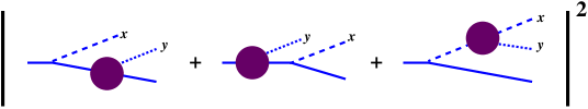
Figure 28: Generalization of Fig. 27 to the total rate.

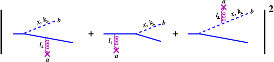
Figure 29: An analogy to Fig. 28: radiation during a high energy, small angle, 2-body collision, where the collision is mediated by exchanging a virtual gauge boson with transverse momentum $l_{\perp}$. The crosses indicate the interaction with the other particle in the 2-body collision, the details of which will not be important here.

What about the condition $k_{\perp}\gg l_{\perp}$ for Gunion-Bertsch cancellation? First consider that for $k_{\perp}\gg l_{\perp}$ and small $x$, the off-shellness $\Delta E$ of energy associated with the intermediate lines in fig. 28 are all of order $k_{\perp}^{2}/xE$, which corresponds to a time scale $\Delta t_{x}\sim xE/k_{\perp}^{2}$. The condition $k_{\perp}\gg l_{\perp}$ is therefore equivalent to the condition $\Delta t_{x}\ll xE/l_{\perp}^{2}$. In the context of fig. 28, $l_{\perp}$ consists of the combination of the transverse momentum carried away by the $y$ bremsstrahlung and the transverse momentum $\sim\sqrt{\hat{q}t_{{\rm form},y}}$ injected by the medium during the $y$ formation, which are parametrically the same and give $l_{\perp}\sim\sqrt{\hat{q}t_{{\rm form},y}}$. So the condition $k_{\perp}\gg l_{\perp}$ is equivalent to

$$\Delta t_{x}\ll\frac{xE}{\hat{q}t_{{\rm form},y}}.$$ (82)

Using the formation time (3), this may be recast as

$$\Delta t_{x}\ll t_{{\rm form},x}\sqrt{\frac{x}{y}}.$$ (83)

Given our original assumption that $y\ll x$, the above condition is automatically satisfied for the range (74) of values that generated the logarithm in our case. The moral of this story is that the logarithms characterized by Table 3 arise from a kinematic regime that is analogous to the cancellation of $k_{\perp}\gg l_{\perp}$ logarithms in Gunion-Bertsch.

B.3 Independent emission model

There is an alternative picture for understanding and interpreting two of the entries in Table 3, which we offer here as a complement to the previous discussion.

B.3.1 The approximation

Imagine that we tried to estimate double bremsstrahlung in the $y\ll x\ll 1$ limit by assuming that the $x$ and $y$ bremsstrahlung amplitudes were completely independent from each other and both given simply by single-bremsstrahlung formulas. This approximation would be somewhat similar to the small $x$ and $y$ limit of the idealized Monte Carlo approximation (19) except that we don’t care about the ordering of $\tau_{x}$ and $\tau_{y}$:

$$\left[\frac{d\Gamma}{dx\,dy}\right]^{\rm independent}\simeq\int_{-\infty}^{\infty}d(\tau_{y}{-}\tau_{x}) \int_{0}^{\infty}d(\Delta t_{\rm x})\int_{0}^{\infty}d(\Delta t_{\rm y})$$

$$\times\operatorname{Re}\left[\frac{d\Gamma}{dx\,d(\Delta t_{\rm x})}\right]_{E}\,\operatorname{Re}\left[\frac{d\Gamma}{dy\,d(\Delta t_{\rm y})}\right]_{E}.$$ (84)

We will find that this is a useful approximation for the processes indicated in the first two rows of Table 3, for which the time integrations above must be correspondingly restricted. (We’ll discuss what happens with the third row of the table later.) In those processes, the $y$ emissions (one in the amplitude and one in the conjugate amplitude) are restricted to occur between the $x$ emissions. This time ordering modifies (84) to

$$\left[\frac{d\Gamma}{dx\,dy}\right]^{\rm independent}_{2\operatorname{Re}(\bullet y\bar{y}\bar{\bullet}+\bullet\bar{y}y\bar{\bullet})}\simeq \int_{0}^{\infty}d(\Delta t_{x})\int_{0}^{\Delta t_{x}}d(\Delta t_{y})\int_{-(\Delta t_{x}-\Delta t_{y})/2}^{+(\Delta t_{x}-\Delta t_{y})/2}d(\tau_{y}{-}\tau_{x})$$

$$\qquad\qquad\times\operatorname{Re}\left[\frac{d\Gamma}{dx\,d(\Delta t_{x})}\right]_{E}\,\operatorname{Re}\left[\frac{d\Gamma}{dy\,d(\Delta t_{y})}\right]_{E}$$

$$= \int_{0}^{\infty}d(\Delta t_{x})\int_{0}^{\Delta t_{x}}d(\Delta t_{y})\>(\Delta t_{x}-\Delta t_{y})$$

$$\qquad\qquad\times\operatorname{Re}\left[\frac{d\Gamma}{dx\,d(\Delta t_{x})}\right]_{E}\,\operatorname{Re}\left[\frac{d\Gamma}{dy\,d(\Delta t_{y})}\right]_{E}.$$ (85)

Why have we written $\bullet y\bar{y}\bar{\bullet}+\bullet\bar{y}y\bar{\bullet}$ in the subscript above instead of, say, $xy\bar{y}\bar{x}+x\bar{y}y\bar{x}$? In our limit $y\ll x\ll 1$, we have $z\equiv 1{-}x{-}y\simeq 1{-}x$. For single bremsstrahlung, there is no difference between referring to the corresponding diagram (fig. 21) as $x\bar{x}$ or $z\bar{z}$ (with $z\equiv 1{-}x$ in the single bremsstrahlung context). We could use either notation to describe the $x$ emission in the independent bremsstrahlung approximation we have outlined above. When we talk about actual double bremsstrahlung diagrams, however, there is a difference. Let’s look at those diagrams: The interference processes listed in the first two rows of Table 3 can be drawn in the form of fig. 30. However, for the reasons given in section IV, we expect that the $y$ emission cannot resolve the two daughters ($x$ and $1{-}x$) of the $x$ emission process when $y\ll x\ll 1$. So $y$ emission from those two daughters is approximately equivalent to $y$ emission from a single particle of energy $E$ (and so is similar to the cases where $y$ emission occurs instead from the initial particle of energy $E$). That is, we can redraw the sum of diagrams in fig. 30 as fig. 31, and it is this sum that should correspond to the independent approximation given by the right-hand side of (85). The subscript notation on the left-hand side of (85) means that this approximation corresponds to the diagrams of fig. 30 with “$\bullet$” summed over the cases $\bullet=x$ and $\bullet=z$.

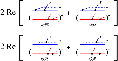
Figure 30: The processes in the first two rows of Table 3, drawn in a way that sets us up for fig. 31. Above, the black dots denote vertices; there is no vertex where lines cross without a dot.

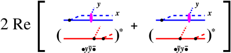
Figure 31: Equivalent to fig. 30 in the limit $y\ll x\ll 1$ where the $y$ emission cannot resolve the $x$ and $1{-}x$ daughters of the $x$ emission process and couples to them (magenta ovals) as to a single adjoint-representation particle.

B.3.2 Evaluation and Comparison

Comparison of (17) and (35) identifies

$$\left[\frac{d\Gamma}{dx\,d(\Delta t)}\right]_{E}=-\frac{\alpha P(x)}{\pi}\,\Omega_{E,x}^{2}\csc^{2}(\Omega_{E,x}\,\Delta t).$$ (86)

Using (63), the independent emission contribution (85) for $y\ll x\ll 1$ is then

$$\left[\frac{d\Gamma}{dx\,dy}\right]^{\rm independent}_{2\operatorname{Re}(\bullet y\bar{y}\bar{\bullet}+\bullet\bar{y}y\bar{\bullet})} \simeq\frac{4C_{\rm A}^{2}\alpha_{\rm s}^{2}}{\pi^{2}xy}\int_{0}^{\infty}d(\Delta t_{y})\>\operatorname{Re}\bigl{[}\Omega_{y}^{2}\csc^{2}(\Omega_{y}\,\Delta t_{y})\bigr{]}$$

$$\qquad\qquad\qquad\times\int_{\Delta t_{y}}^{\infty}d(\Delta t_{x})\>\operatorname{Re}\bigl{[}\Omega_{x}^{2}\csc^{2}(\Omega_{x}\,\Delta t_{x})\bigr{]}\,(\Delta t_{x}-\Delta t_{y})$$

$$=\frac{4C_{\rm A}^{2}\alpha_{\rm s}^{2}}{\pi^{2}xy}\int_{0}^{\infty}d(\Delta t_{y})\>\operatorname{Re}\bigl{[}\Omega_{y}^{2}\csc^{2}(\Omega_{y}\,\Delta t_{y})\bigr{]}\,\operatorname{Re}\ln\left(\frac{1}{1-e^{-2i\Omega_{x}\Delta t_{y}}}\right),$$ (87)

where we define the small $x,y$ expressions

$$\Omega_{x}\equiv\sqrt{-\frac{i\hat{q}_{\rm A}}{2xE}},\qquad\Omega_{y}\equiv\sqrt{-\frac{i\hat{q}_{\rm A}}{2yE}}.$$ (88)

The integrand falls exponentially for $\Delta t_{y}\gg\Omega_{y}^{-1}$, and so $\Omega_{x}\,\Delta t_{y}\ll 1$ in the $y\ll x\ll 1$ limit, giving

$$\left[\frac{d\Gamma}{dx\,dy}\right]^{\rm independent}_{2\operatorname{Re}(\bullet y\bar{y}\bar{\bullet}+\bullet\bar{y}y\bar{\bullet})} \simeq\frac{4C_{\rm A}^{2}\alpha_{\rm s}^{2}}{\pi^{2}xy}\int_{0}^{\infty}d(\Delta t_{y})\>\operatorname{Re}\bigl{[}\Omega_{y}^{2}\csc^{2}(\Omega_{y}\,\Delta t_{y})\bigr{]}\,\operatorname{Re}\ln\left(\frac{1}{2i\Omega_{x}\Delta t_{y}}\right)$$

$$=\frac{4C_{\rm A}^{2}\alpha_{\rm s}^{2}}{\pi^{2}xy}\operatorname{Re}\int_{0}^{\infty}d(\Delta t_{y})\>\Omega_{y}^{2}\csc^{2}(\Omega_{y}\,\Delta t_{y})\,\ln\left(\frac{1}{2|\Omega_{x}|\Delta t_{y}}\right).$$ (89)

This integral has a $\Delta t{\to}0$ divergence. In order to regulate divergences of individual diagrams, we have routinely subtracted out the vacuum contribution to those diagrams. Here, we will subtract out the vacuum contribution to the independent $y$ emission, replacing (89) by

$$\left[\frac{d\Gamma}{dx\,dy}\right]^{\rm independent}_{2\operatorname{Re}(\bullet y\bar{y}\bar{\bullet}+\bullet\bar{y}y\bar{\bullet})} \simeq\frac{4C_{\rm A}^{2}\alpha_{\rm s}^{2}}{\pi^{2}xy}\operatorname{Re}\int_{0}^{\infty}d(\Delta t_{y})\>\left[\Omega_{y}^{2}\csc^{2}(\Omega_{y}\,\Delta t_{y})-\frac{1}{(\Delta t)^{2}}\right]\ln\left(\frac{1}{2|\Omega_{x}|\Delta t_{y}}\right)$$

$$=\frac{4C_{\rm A}^{2}\alpha_{\rm s}^{2}}{\pi^{2}xy}\operatorname{Re}\left\{-i\Omega_{y}\left[\ln\Bigl{(}\frac{i\Omega_{y}}{2\pi|\Omega_{x}|}\Bigr{)}+\gamma_{\rm\scriptscriptstyle E},\right]\right\}$$ (90)

where $\gamma_{\rm\scriptscriptstyle E}$ is the Euler-Mascheroni constant. (We leave a more careful and convincing treatment of the $\Delta t{\to}0$ regularization to other work dimreg .) Using (88), the above result can be recast as

$$\left[\frac{d\Gamma}{dx\,dy}\right]^{\rm independent}_{2\operatorname{Re}(\bullet y\bar{y}\bar{\bullet}+\bullet\bar{y}y\bar{\bullet})}\simeq\frac{C_{\rm A}^{2}\alpha_{\rm s}^{2}}{\pi^{2}xy^{3/2}}\sqrt{\frac{\hat{q}_{\rm A}}{E}}\left[-\ln\Bigl{(}\frac{x}{y}\Bigr{)}+2\ln(2\pi)-2\gamma_{\rm\scriptscriptstyle E}+\frac{\pi}{2}\right].$$ (91)

The coefficient $-1$ of the logarithm indeed matches up with the sum of the first two rows in Table 3, as promised.

We should mention that it is also possible to extract the integral expression in (90) not just from the simple independent bremsstrahlung approximation above but also from the full integral expressions for the general result for $2\operatorname{Re}(xy\bar{y}\bar{x}+x\bar{y}y\bar{x})$ and $2\operatorname{Re}(zy\bar{y}\bar{z}+z\bar{y}y\bar{z})$ given in the preceding work 2brem . This can be done by analytically extracting the behavior of those expressions in the limit $y\ll x\ll 1$ while formally treating the integration variable $\Delta t_{y}\sim\Omega_{y}^{-1}\propto\sqrt{y}$. We will not give details here. Individually, $2\operatorname{Re}(xy\bar{y}\bar{x}+x\bar{y}y\bar{x})$ and $2\operatorname{Re}(zy\bar{y}\bar{z}+z\bar{y}y\bar{z})$ each contribute half of the limiting result (91) in this analysis.

In the first row of Table 3, we did not explicitly list the $2\operatorname{Re}(x\bar{y}\bar{x}y)$ contribution to the group of diagrams represented by $A(x,y)$. To understand this omission, note that the origin of the logarithm in (90) can be traced back to the $\Delta t_{x}-\Delta t_{y}\simeq\Delta t_{x}$ factor inside the last integral in (85). This factor arises because, for $\bullet y\bar{y}\bar{\bullet}+\bullet\bar{y}y\bar{\bullet}$, the short-duration $y$ emission can happen at any time in the middle of the longer-duration $x$ emission. For the $x\bar{y}\bar{x}y$ process shown in fig. 10, however, (and similarly for $z\bar{y}\bar{z}y$) the short-duration $y$ emission is forced by the time-ordering of the diagram to occur only at the very end of the $x$ emission interval, and so there is no comparable factor and so no logarithmic enhancement.

B.3.3 Other processes

One may investigate similar approximations of other processes in Table 3. However, we do not know of any sensible way to apply the independent bremsstrahlung approximation to the third row of the table, which refers to $2\operatorname{Re}(x\bar{z}z\bar{x}+x\bar{z}\bar{x}z+z\bar{x}x\bar{z}+z\bar{x}\bar{z}x)$. These diagrams are depicted in fig. 32 in a fashion similar to fig. 30. These are interference diagrams that combine with the Monte Carlo related diagrams of fig. 33 to partly suppress the result along the lines discussed in section IV. Roughly speaking, the $y$ emission’s inability to individually resolve the $x$ and $1{-}x$ daughters in the $y\ll x$ limit partly suppresses the rate. This combined effect is depicted in fig. 34. The problem with applying an independent bremsstrahlung approximation to the picture in fig. 34, however, is that there is nothing in that approximation that would constrain how large could be the separation of the $y$ emission from the $x$ emission. Consider the two daughters of the $x$ emission. The issue of how $y$ emission from one daughter decoheres with $y$ emission from the other, for times $\gg t_{{\rm form},x}$ after the last $x$ emission, is a complicated matter that is simply not captured by the independent bremsstrahlung approximation that was used so successfully above for fig. 32.

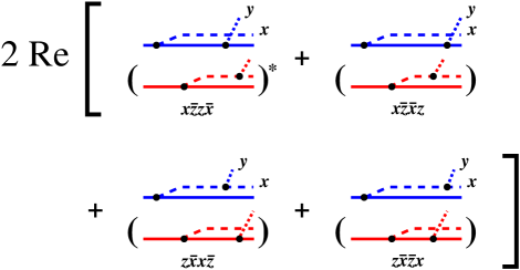
Figure 32: The processes in the third row of Table 3, drawn in a way similar to fig. 30.

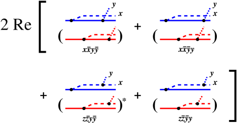
Figure 33: The idealized Monte Carlo related processes associated with the fourth and fifth rows of Table 3, drawn in a way for easy comparison with fig. 32.

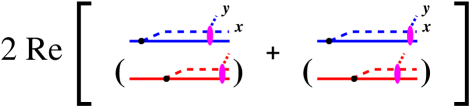
Figure 34: The (problematic) independent bremsstrahlung approximation inspired by the sum of figs. 32 and 33, analogous to fig. 31.

Appendix C More explicit derivation of $x\bar{x}y\bar{y}$

In this appendix, we show how to start with the methods and diagrammatic rules of the preceding paper 2brem and obtain the result for the $x\bar{x}y\bar{y}$ interference given by (29).

Using the notation of ref. 2brem , the $x\bar{x}y\bar{y}$ interference of fig. 35 gives

$$\left[\frac{dI}{dx\,dy}\right]_{x\bar{x}y\bar{y}}=\left(\frac{E}{2\pi}\right)^{2}\int_{t_{\rm x}<t_{\bar{\rm x}}<t_{\rm y}<t_{\bar{\rm y}}}\sum_{\rm pol.}\langle|i\,\overline{\delta H}|{\bm{B}}^{\bar{\rm y}}\rangle\langle{\bm{B}}^{\bar{\rm y}},t_{\bar{\rm y}}|{\bm{B}}^{\rm y},t_{\rm y}\rangle\langle{\bm{B}}^{\rm y}|{-}i\,\delta H|\rangle\\ \times\langle|\rangle^{-1}\langle|i\,\overline{\delta H}|{\bm{B}}^{\bar{\rm x}}\rangle\langle{\bm{B}}^{\bar{\rm x}},t_{\bar{\rm x}}|{\bm{B}}^{\rm x},t_{\rm x}\rangle\langle{\bm{B}}^{\rm x}|{-}i\,\delta H|\rangle$$ (92)

for the differential probability. Here, all transverse positions (${\bm{B}}^{\rm x}$, ${\bm{B}}^{\bar{\rm x}}$, ${\bm{B}}^{\rm y}$, ${\bm{B}}^{\bar{\rm y}}$) are implicitly integrated over, and $\delta H$ is the part of the full Hamiltonian of the theory that contains the splitting vertices for high-energy particles.

Figure 35: Our labeling conventions for times $t_{i}$, longitudinal momenta $x_{i}$ and helicities $h_{i}$ for the $x\bar{x}y\bar{y}$ interference diagram.

One non-trivial normalization factor above has to do with the intermediate 2-particle (effectively 0-particle) state $|\rangle$ for $t_{\bar{\rm x}}<t<t_{\rm y}$. This state was normalized in the preceding paper 2brem as

$$\langle|\rangle=x_{1}^{2}=x_{2}^{2},$$ (93)

where, in this context, $(x_{1},x_{2})=(x_{1},-x_{1})$ are the longitudinal momentum fractions of the two particles in the 2-particle state. This normalization was both natural and convenient in the discussion of ref. 2brem , and it is similarly convenient here, for the normalization of the initial and final states in (92). However, having a non-trivial normalization means that the correct way to project out the 2-particle (effectively 0-particle) intermediate state, appropriate to fig. 35, is with

$$\frac{|\rangle\langle|}{\langle|\rangle}\,,$$ (94)

as in (92).

The effectively 0-particle intermediate state $|\rangle$ does not have any time dependence in our formalism, and so the integrand in (92) does not care how far apart in time $t_{\bar{\rm x}}$ and $t_{\rm y}$ are. That is, we have not bothered to write a factor of 1 in (92) representing the time evolution of this intermediate state:

$$\frac{\langle t_{\rm y}|t_{\bar{\rm x}}\rangle}{\langle|\rangle}=1.$$ (95)

This time independence is consistent with interpreting this diagram as representing two consecutive splittings that are completely independent from each other.

Using the rules developed in the preceding paper 2brem , fig. 35 and (92) become

$$\left[\frac{dI}{dx\,dy}\right]_{x\bar{x}y\bar{y}} =\frac{C_{R}^{2}\alpha_{\rm s}^{2}}{4E^{4}}\,(1-x)^{-2}\int_{t_{\rm x}<t_{\bar{\rm x}}<t_{\rm y}<t_{\bar{\rm y}}}\sum_{h_{\rm x},h_{\rm y},h_{\rm z}}$$

$$\times\Bigl{[}\sum_{\bar{h}}{\cal P}^{\bar{n}}_{\bar{h}\to h_{\rm z},h_{\rm y}}\bigl{(}1{-}x\to 1{-}x{-}y,y\bigr{)}\,{\cal P}^{\bar{m}}_{h_{\rm i}\to\bar{h},h_{\rm x}}\bigl{(}1\to 1{-}x,x\bigr{)}\Bigr{]}^{*}$$

$$\times\Bigl{[}\sum_{h}{\cal P}^{n}_{h\to h_{\rm z},h_{\rm y}}\bigl{(}1{-}x\to 1{-}x{-}y,y\bigr{)}\,{\cal P}^{m}_{h_{\rm i}\to h,h_{\rm x}}\bigl{(}1\to 1{-}x,x\bigr{)}\Bigr{]}$$

$$\times\nabla^{\bar{n}}_{{\bm{B}}^{\bar{\rm y}}}\nabla^{n}_{{\bm{B}}^{\rm y}}\langle{\bm{B}}^{\bar{\rm y}},t_{\bar{\rm y}}|{\bm{B}}^{\rm y},t_{\rm y}\rangle\Bigr{|}_{{\bm{B}}^{\bar{\rm y}}=0={\bm{B}}^{\rm y}}\nabla^{\bar{m}}_{{\bm{B}}^{\bar{\rm x}}}\nabla^{m}_{{\bm{B}}^{\rm x}}\langle{\bm{B}}^{\bar{\rm x}},t_{\bar{\rm x}}|{\bm{B}}^{\rm x},t_{\rm x}\rangle\Bigr{|}_{{\bm{B}}^{\bar{\rm x}}=0={\bm{B}}^{\rm x}},$$ (96)

where ${\cal P}$ is defined in terms of DGLAP splitting functions in section IV.E of ref. 2brem . The overall $(1-x)^{-2}$ factor above is the intermediate-state normalization factor $\langle|\rangle^{-1}$ from (92). In the application in this paper, the color representation $R$ of the solid line in fig. 35 will be adjoint, and so $C_{R}$ above is $C_{\rm A}$.

Now turn to the helicity sums, which we will relate to spin-averaged DGLAP splitting functions. To this end, it is useful to first use rotational invariance in the transverse plane to write

$$\nabla^{\bar{m}}_{{\bm{B}}^{\bar{\rm x}}}\nabla^{m}_{{\bm{B}}^{\rm x}}\langle{\bm{B}}^{\bar{\rm x}},t_{\bar{\rm x}}|{\bm{B}}^{\rm x},t_{\rm x}\rangle\Bigr{|}_{{\bm{B}}^{\bar{\rm x}}=0={\bm{B}}^{\rm x}}=\tfrac{1}{2}\,\delta^{m\bar{m}}{\bm{\nabla}}_{{\bm{B}}^{\bar{\rm x}}}\cdot{\bm{\nabla}}_{{\bm{B}}^{\rm x}}\langle{\bm{B}}^{\bar{\rm x}},t_{\bar{\rm x}}|{\bm{B}}^{\rm x},t_{\rm x}\rangle\Bigr{|}_{{\bm{B}}^{\bar{\rm x}}=0={\bm{B}}^{\rm x}},$$ (97)

and so

$$\left[\frac{dI}{dx\,dy}\right]_{x\bar{x}y\bar{y}} =\frac{C_{R}^{2}\alpha_{\rm s}^{2}}{4E^{4}}\,(1-x)^{-2}\int_{t_{\rm x}<t_{\bar{\rm x}}<t_{\rm y}<t_{\bar{\rm y}}}\tfrac{1}{4}\sum_{h_{\rm x},h_{\rm y},h_{\rm z}}$$

$$\times\Bigl{[}\sum_{\bar{h}}{\cal P}^{n}_{\bar{h}\to h_{\rm z},h_{\rm y}}\bigl{(}1{-}x\to 1{-}x{-}y,y\bigr{)}\,{\cal P}^{m}_{h_{\rm i}\to\bar{h},h_{\rm x}}\bigl{(}1\to 1{-}x,x\bigr{)}\Bigr{]}^{*}$$

$$\times\Bigl{[}\sum_{h}{\cal P}^{n}_{h\to h_{\rm z},h_{\rm y}}\bigl{(}1{-}x\to 1{-}x{-}y,y\bigr{)}\,{\cal P}^{m}_{h_{\rm i}\to h,h_{\rm x}}\bigl{(}1\to 1{-}x,x\bigr{)}\Bigr{]}$$

$$\times{\bm{\nabla}}_{{\bm{B}}^{\bar{\rm y}}}\cdot{\bm{\nabla}}_{{\bm{B}}^{\rm y}}\langle{\bm{B}}^{\bar{\rm y}},t_{\bar{\rm y}}|{\bm{B}}^{\rm y},t_{\rm y}\rangle\Bigr{|}_{{\bm{B}}^{\bar{\rm y}}=0={\bm{B}}^{\rm y}}{\bm{\nabla}}_{{\bm{B}}^{\bar{\rm x}}}\cdot{\bm{\nabla}}_{{\bm{B}}^{\rm x}}\langle{\bm{B}}^{\bar{\rm x}},t_{\bar{\rm x}}|{\bm{B}}^{\rm x},t_{\rm x}\rangle\Bigr{|}_{{\bm{B}}^{\bar{\rm x}}=0={\bm{B}}^{\rm x}}.$$ (98)

By reflection invariance of the problem in the transverse plane, we are free to average over initial helicities $h_{\rm i}$. The factor

$$\sum_{h_{\rm x},h_{\rm y},h_{\rm z}}\Bigl{[}\sum_{\bar{h}}{\cal P}^{n}_{\bar{h}\to h_{\rm z},h_{\rm y}}{\cal P}^{m}_{h_{\rm i}\to\bar{h},h_{\rm x}}\Bigr{]}^{*}\Bigl{[}\sum_{h}{\cal P}^{n}_{h\to h_{\rm z},h_{\rm y}}{\cal P}^{m}_{h_{\rm i}\to h,h_{\rm x}}\Bigr{]}$$ (99)

(where we’ve suppressed the other arguments of ${\cal P}$ for brevity) then becomes

$$\tfrac{1}{2}\sum_{h,\bar{h}}\Bigl{[}\sum_{h_{\rm y},h_{\rm z}}{\bm{\mathcal{P}}}_{\bar{h}\to h_{\rm z},h_{\rm y}}^{*}\cdot{\bm{\mathcal{P}}}_{h\to h_{\rm z},h_{\rm y}}\sum_{h_{\rm i},h_{\rm x}}{\bm{\mathcal{P}}}_{h_{\rm i}\to\bar{h},h_{\rm x}}^{*}\cdot{\bm{\mathcal{P}}}_{h_{\rm i}\to h,h_{\rm x}}\Bigr{]}.$$ (100)

By rotational invariance, $\sum_{h_{\rm y},h_{\rm z}}{\bm{\mathcal{P}}}_{\bar{h}\to h_{\rm z},h_{\rm y}}^{*}\cdot{\bm{\mathcal{P}}}_{h\to h_{\rm z},h_{\rm y}}=\tfrac{1}{2}\delta_{h,\bar{h}}\sum_{h^{\prime},h_{\rm y},h_{\rm z}}{\bm{\mathcal{P}}}_{h^{\prime}\to h_{\rm z},h_{\rm y}}^{*}\cdot{\bm{\mathcal{P}}}_{h^{\prime}\to h_{\rm z},h_{\rm y}}$, and (100) becomes

$$\tfrac{1}{2}\sum_{h^{\prime},h_{\rm y},h_{\rm z}}{\bm{\mathcal{P}}}_{h^{\prime}\to h_{\rm z},h_{\rm y}}^{*}\cdot{\bm{\mathcal{P}}}_{h^{\prime}\to h_{\rm z},h_{\rm y}}\times\tfrac{1}{2}\sum_{h_{\rm i},h,h_{\rm x}}{\bm{\mathcal{P}}}_{h_{\rm i}\to h,h_{\rm x}}^{*}\cdot{\bm{\mathcal{P}}}_{h_{\rm i}\to h,h_{\rm x}}.$$ (101)

Up to normalization factors in the definition of ${\bm{\mathcal{P}}}$, the two factors above each represent a spin-averaged DGLAP splitting function. Taking the precise definition of ${\bm{\mathcal{P}}}$ from the preceding paper 2brem , we specifically obtain

$$\frac{2\,P\bigl{(}-(1{-}x),1{-}x{-}y,y\bigr{)}}{C_{R}(1{-}x)^{2}y^{2}(1{-}x{-}y)^{2}}\times\frac{2\,P(-1,1{-}x,x)}{C_{R}x^{2}(1{-}x)^{2}}=\frac{2\,P({\mathfrak{y}})}{C_{R}(1{-}x)y^{2}(1{-}x{-}y)^{2}}\times\frac{2\,P(x)}{C_{R}x^{2}(1{-}x)^{2}}\,.$$ (102)

Substituting (102) for (99) in (98) then yields

$$\left[\frac{dI}{dx\,dy}\right]_{x\bar{x}y\bar{y}} =(1-x)^{-1}\int_{t_{\rm x}<t_{\bar{\rm x}}<t_{\rm y}<t_{\bar{\rm y}}}$$

$$\times\frac{\alpha_{\rm s}P({\mathfrak{y}})}{2[(1-x)y(1-x-y)E]^{2}}\,{\bm{\nabla}}_{{\bm{B}}^{\bar{\rm y}}}\cdot{\bm{\nabla}}_{{\bm{B}}^{\rm y}}\langle{\bm{B}}^{\bar{\rm y}},t_{\bar{\rm y}}|{\bm{B}}^{\rm y},t_{\rm y}\rangle\Bigr{|}_{{\bm{B}}^{\bar{\rm y}}=0={\bm{B}}^{\rm y}}$$

$$\times\frac{\alpha_{\rm s}P(x)}{2[x(1-x)E]^{2}}\,{\bm{\nabla}}_{{\bm{B}}^{\bar{\rm x}}}\cdot{\bm{\nabla}}_{{\bm{B}}^{\rm x}}\langle{\bm{B}}^{\bar{\rm x}},t_{\bar{\rm x}}|{\bm{B}}^{\rm x},t_{\rm x}\rangle\Bigr{|}_{{\bm{B}}^{\bar{\rm x}}=0={\bm{B}}^{\rm x}}$$ (103)

with ${\mathfrak{y}}$ defined by (12).

Now using the definition (18) of $d\Gamma/dx\,d\Delta t$, (103) will give (once we clarify below some issues about normalization)

$$\left[\frac{dI}{dx\,dy}\right]_{x\bar{x}y\bar{y}}=(1-x)^{-1} \int_{t_{\rm x}<t_{\bar{\rm x}}<t_{\rm y}<t_{\bar{\rm y}}}dt_{\rm x}\,dt_{\bar{\rm x}}\,dt_{\rm y}\,dt_{\bar{\rm y}}$$

$$\times\frac{1}{2}\left[\frac{d\Gamma}{d{\mathfrak{y}}\,d(\Delta t_{\rm y})}\right]_{(1-x)E}\,\frac{1}{2}\left[\frac{d\Gamma}{dx\,d(\Delta t_{\rm x})}\right]_{E},$$ (104)

which is the result claimed in (29) in the main text (after using time translation invariance to eliminate one of the time integrals and so change probability distribution $dI/dx\,dy$ to rate distribution $d\Gamma/dx\,dy$).

Let’s now address the normalization issue, since (103) and (104) may not look like they exactly match up. In particular, one might think that the formula for $[d\Gamma/d{\mathfrak{y}}\,\Delta t]_{(1-x)E}$ is obtained from the definition (18) of $[d\Gamma/dx\,d\Delta t]_{E}$ by simply substituting $\bigl{(}(1-x)E,{\mathfrak{y}}\bigr{)}$ for $(E,x)$. But this overlooks the fact that the effective 1-particle quantum mechanics variables ${\bm{B}}$ here and in the previous paper 2brem are defined using the longitudinal momentum fractions defined with respect to the initial parent $E$ of the full double-splitting process. In the case of the $t_{\rm y}<t<t_{\bar{\rm y}}$ evolution in fig. 35 and (96),

$${\bm{B}}=\frac{{\bm{b}}_{z}-{\bm{b}}_{y}}{z+y}=\frac{{\bm{b}}_{z}-{\bm{b}}_{y}}{1{-}x},$$ (105)

where ${\bm{b}}_{z}$ and ${\bm{b}}_{y}$ are the transverse positions of the $z$ and $y$ daughters. In contrast, the ${\bm{B}}$ in the corresponding single-splitting calculation would be

$${\mathfrak{B}}\equiv\frac{{\bm{b}}_{1-{\mathfrak{y}}}-{\bm{b}}_{\mathfrak{y}}}{(1{-}{\mathfrak{y}})+{\mathfrak{y}}}={\bm{b}}_{1-{\mathfrak{y}}}-{\bm{b}}_{\mathfrak{y}},$$ (106)

which is (other than the choice of notation) the same thing as ${\bm{b}}_{z}-{\bm{b}}_{y}$. The correct translation of (18) is then

$$\left[\frac{d\Gamma}{d{\mathfrak{y}}\,d(\Delta t)}\right]_{(1-x)E}=\frac{\alpha_{\rm s}P({\mathfrak{y}})}{[{\mathfrak{y}}(1-{\mathfrak{y}})(1-x)E]^{2}}{\bm{\nabla}}_{{\mathfrak{B}}^{\bar{\rm y}}}\cdot{\bm{\nabla}}_{{\mathfrak{B}}^{\rm y}}\langle{\mathfrak{B}}^{\bar{\rm y}},\Delta t|{\mathfrak{B}}^{\rm y},0\rangle_{E,x}\Bigr{|}_{{\mathfrak{B}}^{\bar{\rm y}}=0={\mathfrak{B}}^{\rm y}}.$$ (107)

Recalling that the states $|{\bm{B}}\rangle$ are normalized so that $\langle{\bm{B}}|{\bm{B}}^{\prime}\rangle=\delta^{(2)}({\bm{B}}-{\bm{B}}^{\prime})$ [and so correspondingly $\langle{\mathfrak{B}}|{\mathfrak{B}}^{\prime}\rangle=\delta^{(2)}({\mathfrak{B}}-{\mathfrak{B}}^{\prime})$], the relationship ${\mathfrak{B}}=(1-x){\bm{B}}$ between (105) and (106) lets us rewrite (107) as

$$\left[\frac{d\Gamma}{d{\mathfrak{y}}\,d(\Delta t)}\right]_{(1-x)E}=\frac{\alpha_{\rm s}P({\mathfrak{y}})}{[(1-x)y(1-x-y)E]^{2}}\,{\bm{\nabla}}_{{\bm{B}}^{\bar{\rm y}}}\cdot{\bm{\nabla}}_{{\bm{B}}^{\rm y}}\langle{\bm{B}}^{\bar{\rm y}},t_{\bar{\rm y}}|{\bm{B}}^{\rm y},t_{\rm y}\rangle\Bigr{|}_{{\bm{B}}^{\bar{\rm y}}=0={\bm{B}}^{\rm y}}.$$ (108)

This indeed matches up with the corresponding factor in (103) to give (104).

Appendix D Justification of the prescription (26)

We now outline how to justify the midpoint prescription (26). As discussed in the main text, the starting point is to imagine a medium with, for example,

$$\hat{q}(t)=\hat{q}_{0}\,e^{-t^{2}/\mathbb{T}^{2}}.$$ (109)

In the limit of large $\mathbb{T}$, $\hat{q}$ is approximately constant over any formation time, and so we may still analyze the effects of overlapping formation times in the constant-$\hat{q}$ approximation used for detailed calculations in this paper. But, at the same time, (109) helps by providing a consistent large-time regulator for independent splittings that are far separated in time.

There is a subtlety, however, to approximating $\hat{q}$ as constant over formation times. Consider, formally, the contribution of $x\bar{x}y\bar{y}$ to the total probability $I$ for double splitting:

$$\left[\frac{dI}{dx\,dy}\right]_{x\bar{x}y\bar{y}}=\frac{1}{1-x} \int_{t_{\rm x}<t_{\bar{\rm x}}<t_{\rm y}<t_{\bar{\rm y}}}\!dt_{\rm x}\,dt_{\bar{\rm x}}\,dt_{\rm y}\,dt_{\bar{\rm y}}$$

$$\times\tfrac{1}{2}\left[\frac{d\Gamma}{dx\,d(\Delta t_{\rm x})}\right]_{E}\,\tfrac{1}{2}\left[\frac{d\Gamma}{d{\mathfrak{y}}\,d(\Delta t_{\rm y})}\right]_{(1-x)E}.$$ (110)

When evaluating $d\Gamma/d{\mathfrak{y}}\,d\Delta t_{\rm y}$ in the integrand, should we take $\hat{q}$ to be $\hat{q}(t_{\rm y})$ or $\hat{q}(t_{\bar{\rm y}})$ or pick some other time in between? [A similar question arises for $d\Gamma/dx\,d\Delta t_{\rm x}$.] This may at first sound unimportant because the integrand falls off exponentially when $\Delta t_{\rm y}$ exceeds the formation time, and so (except for negligible corrections) $t_{\rm y}$ and $t_{\bar{\rm y}}$ can be at most roughly a formation time apart. That means $\hat{q}(t_{\rm y})\to\hat{q}(t_{\bar{\rm y}})$ as $\mathbb{T}\to\infty$. The difference between $\hat{q}(t_{\rm y})$ and $\hat{q}(t_{\bar{\rm y}})$, and so the different values we might get for $d\Gamma/d{\mathfrak{y}}\,d\Delta t_{\rm y}$, scale at worst like $\mathbb{T}^{-1}$. The problem is that this correction can accumulate additively when we integrate over time. For simplicity of argument, let’s focus on the integral over $t_{\rm y}$ while holding $t_{\rm x}$, $t_{\bar{\rm x}}$, and $\Delta t_{\rm y}\equiv t_{\bar{\rm y}}-t_{\rm y}$ fixed. If we choose to evaluate $\hat{q}$ at $t_{\rm y}$, then the $dt_{\rm y}$ integral has the functional form

$$\int_{t_{\bar{\rm x}}}^{\infty}dt_{\rm y}\>f\bigl{(}\hat{q}(t_{\rm y})\bigr{)}$$ (111)

for some function $f(\hat{q})$. If we instead take $\hat{q}(t_{\bar{\rm y}})$, it is

$$\int_{t_{\bar{\rm x}}}^{\infty}dt_{\rm y}\>f\bigl{(}\hat{q}(t_{\rm y}+\Delta t_{\rm y})\bigr{)}=\int_{t_{\bar{\rm x}}+\Delta t_{\rm y}}^{\infty}dt_{\bar{\rm y}}f\bigl{(}\hat{q}(t_{\bar{\rm y}})\bigr{)}.$$ (112)

The difference between these two prescriptions is

$$\int_{t_{\bar{\rm x}}}^{t_{\bar{\rm x}}+\Delta t_{\rm y}}dt\>f\bigl{(}\hat{q}(t)\bigr{)},$$ (113)

which does not vanish as $\mathbb{T}\to\infty$, and so the difference of the prescriptions for $\hat{q}$ cannot be ignored.

So which choice is correct? We could avoid this question by computing $d\Gamma/d{\mathfrak{y}}\,d\Delta t_{\rm y}$ [and similarly $d\Gamma/dx\,d\Delta t_{\rm x}$] without making the approximation that $\hat{q}$ is constant over $\Delta t$, but that makes the calculation unnecessarily difficult. Instead, consider the following. For simplicity of argument, focus on a region of time where $\hat{q}(t)$ is monotonically decreasing, i.e. $t>0$ in (109). The problem with the choice $\hat{q}(t_{\rm y})$ for the time interval $(t_{\rm y},t_{\bar{\rm y}})$ is then that it overestimates $\hat{q}(t)$ for the entire interval. The problem with the choice $\hat{q}(t_{\bar{\rm y}})$ is that it underestimates $\hat{q}(t)$ for the entire interval. However, if we choose the mid-point, $\hat{q}(\tau_{\rm y})$ with $\tau_{\rm y}\equiv(t_{\rm y}+t_{\bar{\rm y}})/2$, we will in almost equal measure overestimate $\hat{q}$ in the first half of the interval and underestimate it in the second half. That is, the error we make in $d\Gamma/d{\mathfrak{y}}\,d\Delta t_{\rm y}$ will be $O(\mathbb{T}^{-2})$ instead of $O(\mathbb{T}^{-1})$. This is small enough that the accumulated error after integrating $t_{\rm y}$ over time will not affect our final results in the $\mathbb{T}\to\infty$ limit.

The upshot is that, in the $x\bar{x}y\bar{y}$ calculation, $\hat{q}$ should be evaluated at the midpoint times $\tau_{\rm x}$ and $\tau_{\rm y}$. In the single-splitting calculation, it should also be evaluated at the midpoint time, and so the formula used for the idealized Monte Carlo calculation also corresponds to using $\hat{q}(\tau_{\rm x})$ and $\hat{q}(\tau_{\rm y})$, where $\tau_{\rm x}$ and $\tau_{\rm y}$ are the emission times in the idealized Monte Carlo. We could now go through all the steps from (28) to (34) explicitly specifying the use of $\hat{q}(\tau_{\rm x})$ and $\hat{q}(\tau_{\rm y})$. However, once we get to the final result (34), which is finite as $\mathbb{T}\to\infty$, we no longer have to worry about this distinction. We can then simply take $\mathbb{T}\to\infty$ and call $\hat{q}$ a constant.

Appendix E Derivation of $xy\bar{x}\bar{y}_{2}$

E.1 Basics

In this appendix, we step through the derivation of the result (47) for the $xy\bar{x}\bar{y}_{2}$ interference contribution of fig. 24. Our notation is given in fig. 36.

Figure 36: Our labeling conventions for the $xy\bar{x}\bar{y}_{2}$ interference diagram. (The only difference between $xy\bar{x}\bar{y}_{2}$ and $xy\bar{x}\bar{y}_{1}$ is the order $(x_{1},x_{2},x_{3},x_{4})$ we have chosen for labeling the particles during the 4-particle evolution $t_{\rm y}<t<t_{\bar{\rm x}}$.)

A direct application of the methods of the preceding paper 2brem gives (remembering that $\hat{x}_{1}+\hat{x}_{4}=-\hat{x}_{2}-\hat{x}_{3}$)

$$\left[\frac{dI}{dx\,dy}\right]_{xy\bar{x}\bar{y}_{2}} =\tfrac{1}{2}C_{\rm A}^{2}\,\frac{\alpha_{\rm s}^{2}}{4E^{4}}\,(\hat{x}_{1}+\hat{x}_{4})^{-2}\int_{t_{\rm x}<t_{\rm y}<t_{\bar{\rm x}}<t_{\bar{\rm y}}}\int_{{\bm{B}}^{\rm y},{\bm{B}}^{\bar{\rm x}}}\sum_{h_{\rm x},h_{\rm y},h_{\rm z}}$$

$$\times\Bigl{[}\sum_{\bar{h}}{\cal P}^{\bar{n}}_{\bar{h}\to h_{\rm z},h_{\rm y}}\bigl{(}1{-}x\to 1{-}x{-}y,y\bigr{)}\,{\cal P}^{\bar{m}}_{h_{\rm i}\to\bar{h},h_{\rm x}}\bigl{(}1\to 1{-}x,x\bigr{)}\Bigr{]}^{*}$$

$$\times\Bigl{[}\sum_{h}{\cal P}^{n}_{h\to h_{\rm z},h_{\rm y}}\bigl{(}1{-}x\to 1{-}x{-}y,y\bigr{)}\,{\cal P}^{m}_{h_{\rm i}\to h,h_{\rm x}}\bigl{(}1\to 1{-}x,x\bigr{)}\Bigr{]}$$

$$\times\nabla^{\bar{n}}_{{\bm{B}}^{\bar{\rm y}}}\langle{\bm{B}}^{\bar{\rm y}},t_{\bar{\rm y}}|{\bm{B}}^{\bar{\rm x}},t_{\bar{\rm x}}\rangle\Bigr{|}_{{\bm{B}}^{\bar{\rm y}}=0}$$

$$\times\nabla^{\bar{m}}_{{\bm{C}}_{41}^{\bar{\rm x}}}\nabla^{n}_{{\bm{C}}_{23}^{\rm y}}\langle{\bm{C}}_{41}^{\bar{\rm x}},{\bm{C}}_{23}^{\bar{\rm x}},t_{\bar{\rm x}}|{\bm{C}}_{41}^{\rm y},{\bm{C}}_{23}^{\rm y},t_{\rm y}\rangle\Bigr{|}_{{\bm{C}}_{41}^{\bar{\rm x}}=0={\bm{C}}_{23}^{\rm y};~{}{\bm{C}}_{23}^{\bar{\rm x}}={\bm{B}}^{\bar{\rm x}};~{}{\bm{C}}_{41}^{\rm y}={\bm{B}}^{\rm y}}$$

$$\times\nabla^{m}_{{\bm{B}}^{\rm x}}\langle{\bm{B}}^{\rm y},t_{\rm y}|{\bm{B}}^{\rm x},t_{\rm x}\rangle\Bigr{|}_{{\bm{B}}^{\rm x}=0}.$$ (114)

The color factor $\frac{1}{2}C_{\rm A}^{2}$ in front is half of the naive color factor $d_{\rm A}^{-1}\operatorname{tr}(T^{a}_{\rm A}T^{a}_{\rm A}T^{b}_{\rm A}T^{b}_{\rm A})=C_{\rm A}^{2}$ from the drawing of fig. 36 because $xy\bar{x}\bar{y}_{2}$ given by (114) represents the contribution from only one of the two large-$N_{\rm c}$ color routings of $xy\bar{x}\bar{y}$.

The helicity sums are not as simple as in the $x\bar{x}y\bar{y}$ case of appendix C because we do not have any useful analog of (97) to start the simplification. However, we may again average over the initial helicity $h_{\rm i}$, and rotational symmetry in the transverse plane implies that the initial helicity average of

$$\sum_{h_{\rm x},h_{\rm y},h_{\rm z}} \Bigl{[}\sum_{\bar{h}}{\cal P}^{\bar{n}}_{\bar{h}\to h_{\rm z},h_{\rm y}}\bigl{(}1{-}x\to 1{-}x{-}y,y\bigr{)}\,{\cal P}^{\bar{m}}_{h_{\rm i}\to\bar{h},h_{\rm x}}\bigl{(}1\to 1{-}x,x\bigr{)}\Bigr{]}^{*}$$

$$\times \Bigl{[}\sum_{h}{\cal P}^{n}_{h\to h_{\rm z},h_{\rm y}}\bigl{(}1{-}x\to 1{-}x{-}y,y\bigr{)}\,{\cal P}^{m}_{h_{\rm i}\to h,h_{\rm x}}\bigl{(}1\to 1{-}x,x\bigr{)}\Bigr{]}$$ (115)

above must have the form

$$\bar{\alpha}(x,y)\,\delta^{\bar{n}n}\delta^{\bar{m}m}+\bar{\beta}(x,y)\,\delta^{\bar{n}\bar{m}}\delta^{nm}+\bar{\gamma}(x,y)\,\delta^{\bar{n}m}\delta^{n\bar{m}},$$ (116)

for some functions $\bar{\alpha}$, $\bar{\beta}$, and $\bar{\gamma}$, analogous to eq. (4.38) of ref. 2brem . Using the explicit formulas for the ${\cal P}$’s for the case where all high-energy particles are gluons, we find

$$\begin{pmatrix}\bar{\alpha}\\ \bar{\beta}\\ \bar{\gamma}\end{pmatrix}_{x\bar{y}\bar{x}y}=\phantom{+} \begin{pmatrix}-\\ +\\ +\end{pmatrix}\frac{4}{xy(1{-}x)^{6}(1{-}x{-}y)}$$

$$+ \begin{pmatrix}+\\ -\\ +\end{pmatrix}\Biggl{[}\frac{1}{x^{3}y^{3}(1{-}x)^{2}(1{-}x{-}y)^{3}}+\frac{1{-}x{-}y}{x^{3}y^{3}(1{-}x)^{2}}$$

$$\qquad\qquad+\frac{x}{y^{3}(1{-}x)^{2}(1{-}x{-}y)^{3}}+\frac{y}{x^{3}(1{-}x)^{2}(1{-}x{-}y)^{3}}\Biggr{]}$$

$$+ \begin{pmatrix}+\\ +\\ -\end{pmatrix}\Biggl{[}\frac{(1{-}x)^{2}}{x^{3}y^{3}(1{-}x{-}y)^{3}}+\frac{(1{-}x{-}y)}{x^{3}y^{3}(1{-}x)^{6}}+\frac{x(1{-}x{-}y)}{y^{3}(1{-}x)^{6}}$$

$$\qquad\qquad+\frac{y}{x^{3}(1{-}x)^{6}(1{-}x{-}y)^{3}}+\frac{xy}{(1{-}x)^{6}(1{-}x{-}y)^{3}}\Biggr{]}.$$ (117)

It will be useful to note for future reference that a certain combination of $(\bar{\alpha},\bar{\beta},\bar{\gamma})$ can be written in terms of spin-averaged DGLAP splitting functions:

$$\bar{\alpha}+\tfrac{1}{2}\bar{\beta}+\tfrac{1}{2}\bar{\gamma} =\frac{[1+x^{4}+(1{-}x)^{4}]}{x^{3}(1{-}x)^{3}}\,\frac{[(1{-}x)^{4}+y^{4}+(1{-}x{-}y)^{4}]}{(1{-}x)^{3}y^{3}(1{-}x{-}y)^{3}}$$

$$=\frac{P(x)}{C_{\rm A}x^{2}(1{-}x)^{2}}\,\,\frac{P\bigl{(}\frac{y}{1{-}x}\bigr{)}}{C_{\rm A}(1{-}x)y^{2}(1{-}x{-}y)^{2}}\,.$$ (118)

Replacing (115) by (116) in (114) gives

$$\left[\frac{dI}{dx\,dy}\right]_{xy\bar{x}\bar{y}_{2}} =\frac{C_{\rm A}^{2}\alpha_{\rm s}^{2}}{8E^{4}}\,\frac{(\bar{\alpha}\delta^{\bar{n}n}\delta^{\bar{m}m}{+}\bar{\beta}\delta^{\bar{n}\bar{m}}\delta^{nm}{+}\bar{\gamma}\delta^{\bar{n}m}\delta^{n\bar{m}})}{|\hat{x}_{1}+\hat{x}_{4}|^{2}}\int_{t_{\rm x}<t_{\rm y}<t_{\bar{\rm x}}<t_{\bar{\rm y}}}\int_{{\bm{B}}^{\rm y},{\bm{B}}^{\bar{\rm x}}}$$

$$\times\nabla^{\bar{n}}_{{\bm{B}}^{\bar{\rm y}}}\langle{\bm{B}}^{\bar{\rm y}},t_{\bar{\rm y}}|{\bm{B}}^{\bar{\rm x}},t_{\bar{\rm x}}\rangle\Bigr{|}_{{\bm{B}}^{\bar{\rm y}}=0}$$

$$\times\nabla^{\bar{m}}_{{\bm{C}}_{41}^{\bar{\rm x}}}\nabla^{n}_{{\bm{C}}_{23}^{\rm y}}\langle{\bm{C}}_{41}^{\bar{\rm x}},{\bm{C}}_{23}^{\bar{\rm x}},t_{\bar{\rm x}}|{\bm{C}}_{41}^{\rm y},{\bm{C}}_{23}^{\rm y},t_{\rm y}\rangle\Bigr{|}_{{\bm{C}}_{41}^{\bar{\rm x}}=0={\bm{C}}_{23}^{\rm y};~{}{\bm{C}}_{23}^{\bar{\rm x}}={\bm{B}}^{\bar{\rm x}};~{}{\bm{C}}_{41}^{\rm y}={\bm{B}}^{\rm y}}$$

$$\times\nabla^{m}_{{\bm{B}}^{\rm x}}\langle{\bm{B}}^{\rm y},t_{\rm y}|{\bm{B}}^{\rm x},t_{\rm x}\rangle\Bigr{|}_{{\bm{B}}^{\rm x}=0}.$$ (119)

E.2 Multiple scattering ($\hat{q}$) approximation

In the harmonic oscillator approximation, we may do the first and last time integrals ($t_{\bm{x}}$ and $t_{\bar{\rm y}}$) as in section V.A of ref. 2brem , with result

$$\left[\frac{d\Gamma}{dx\,dy}\right]_{xy\bar{x}\bar{y}_{2}} =-\frac{C_{\rm A}^{2}\alpha_{\rm s}^{2}M_{\rm i}M_{\rm f}^{\rm seq}}{8\pi^{2}E^{4}}\,\frac{(\bar{\alpha}\delta^{\bar{n}n}\delta^{\bar{m}m}{+}\bar{\beta}\delta^{\bar{n}\bar{m}}\delta^{nm}{+}\bar{\gamma}\delta^{\bar{n}m}\delta^{n\bar{m}})}{|\hat{x}_{1}+\hat{x}_{4}|^{2}}$$

$$\quad\times\int_{0}^{\infty}d(\Delta t)\int_{{\bm{B}}^{\rm y},{\bm{B}}^{\bar{\rm x}}}\frac{B^{{\bar{\rm x}}}_{\bar{n}}}{(B^{\bar{\rm x}})^{2}}\,\frac{B^{{\rm y}}_{m}}{(B^{\rm y})^{2}}\,\exp\bigl{(}-\tfrac{1}{2}|M_{\rm f}^{\rm seq}|\Omega_{\rm f}^{\rm seq}(B^{\bar{\rm x}})^{2}-\tfrac{1}{2}|M_{\rm i}|\Omega_{\rm i}(B^{\rm y})^{2}\bigr{)}$$

$$\qquad\times\nabla^{\bar{m}}_{{\bm{C}}_{41}^{\bar{\rm x}}}\nabla^{n}_{{\bm{C}}_{23}^{\rm y}}\langle{\bm{C}}_{41}^{\bar{\rm x}},{\bm{C}}_{23}^{\bar{\rm x}},t_{\bar{\rm x}}|{\bm{C}}_{41}^{\rm y},{\bm{C}}_{23}^{\rm y},t_{\rm y}\rangle\Bigr{|}_{{\bm{C}}_{41}^{\bar{\rm x}}=0={\bm{C}}_{23}^{\rm y};~{}{\bm{C}}_{23}^{\bar{\rm x}}={\bm{B}}^{\bar{\rm x}};~{}{\bm{C}}_{41}^{\rm y}={\bm{B}}^{\rm y}},$$ (120)

where $\Delta t\equiv t_{\bar{\rm x}}-t_{\rm y}$ and

$$M_{\rm i}=\hat{x}_{1}\hat{x}_{4}(\hat{x}_{1}{+}\hat{x}_{4})E,\qquad M_{\rm f}^{\rm seq}=\hat{x}_{2}\hat{x}_{3}(\hat{x}_{2}{+}\hat{x}_{3})E.$$ (121)

$\Omega_{\rm i}$ and $\Omega_{\rm f}^{\rm seq}$ are respectively the $\Omega_{E,x}$ and $\Omega_{(1-x)E,{\mathfrak{y}}}$ of (36) and (38). We put the superscript “seq” on $M_{\rm f}^{\rm seq}$ and $\Omega_{\rm f}^{\rm seq}$ to indicate that they are different than the corresponding $M_{\rm f}$ and $\Omega_{\rm f}$ in the calculation of the canonical diagram $xy\bar{y}\bar{x}$ in ref. 2brem .

Unlike in the $xy\bar{y}\bar{x}$ analysis of the preceding paper 2brem , the relevant variables $({\bm{C}}_{41},{\bm{C}}_{23})$ are the same on both sides of $\langle{\bm{C}}_{41}^{\bar{\rm x}},{\bm{C}}_{23}^{\bar{\rm x}},t_{\bar{\rm x}}|{\bm{C}}_{41}^{\rm y},{\bm{C}}_{23}^{\rm y},t_{\rm y}\rangle$ above. In order to keep the notation similar to that of the preceding paper, it is useful to consider the variables ordered on the two ends as

$$\begin{pmatrix}{\bm{C}}^{\bar{\rm x}}_{23}\\ {\bm{C}}^{\bar{\rm x}}_{41}\end{pmatrix}\qquad\mbox{and}\qquad\begin{pmatrix}{\bm{C}}^{\rm y}_{41}\\ {\bm{C}}^{\rm y}_{23}\end{pmatrix}$$ (122)

so that the derivatives in (120) hit the lower element of each pair (as in that paper). The appropriate transformation matrix between these variables and the normal modes for the 4-particle evolution is

$$a_{\rm y}\equiv\begin{pmatrix}C^{+}_{41}&C^{-}_{41}\\ C^{+}_{23}&C^{-}_{23}\end{pmatrix}$$ (123)

at $t_{\rm y}$, in the notation of the preceding paper. The explicit formula is given by eqs. (5.24,5.28,5.33) of that paper. Given the choice (122), the corresponding transformation at $t_{\bar{\rm x}}$ is simply

$$a_{\bar{\rm x}}^{\rm seq}\equiv\begin{pmatrix}0&1\\ 1&0\end{pmatrix}a_{\rm y}.$$ (124)

The rest of the analysis proceeds as in section V.C of ref. 2brem but using

$$\begin{pmatrix}X_{\rm y}^{\rm seq}&Y_{\rm y}^{\rm seq}\\ Y_{\rm y}^{\rm seq}&Z_{\rm y}^{\rm seq}\end{pmatrix} \equiv\begin{pmatrix}|M_{\rm i}|\Omega_{\rm i}&0\\ 0&0\end{pmatrix}-ia_{\rm y}^{-1\top}\underline{\Omega}\cot(\underline{\Omega}\,\Delta t)\,a_{\rm y}^{-1}=\begin{pmatrix}X_{\rm y}&Y_{\rm y}\\ Y_{\rm y}&Z_{\rm y}\end{pmatrix},$$ (125a)

$$\begin{pmatrix}X_{\bar{\rm x}}^{\rm seq}&Y_{\bar{\rm x}}^{\rm seq}\\ Y_{\bar{\rm x}}^{\rm seq}&Z_{\bar{\rm x}}^{\rm seq}\end{pmatrix} \equiv\begin{pmatrix}|M_{\rm f}^{\rm seq}|\Omega_{\rm f}^{\rm seq}&0\\ 0&0\end{pmatrix}-i(a_{\bar{\rm x}}^{\rm seq})^{-1\top}\underline{\Omega}\cot(\underline{\Omega}\,\Delta t)\,(a_{\bar{\rm x}}^{\rm seq})^{-1},$$ (125b)

$$\begin{pmatrix}X_{{\rm y}{\bar{\rm x}}}^{\rm seq}&Y_{{\rm y}{\bar{\rm x}}}^{\rm seq}\\ \overline{Y}_{{\rm y}{\bar{\rm x}}}^{\rm seq}&Z_{{\rm y}{\bar{\rm x}}}^{\rm seq}\end{pmatrix} \equiv-ia_{\rm y}^{-1\top}\underline{\Omega}\csc(\underline{\Omega}\,\Delta t)\,(a_{\bar{\rm x}}^{\rm seq})^{-1}$$ (125c)

in result (47) of this paper. The $I^{\rm seq}$’s in (47) are defined the same way as the $I$’s of ref. 2brem but using the appropriate $(X^{\rm seq},Y^{\rm seq},Z^{\rm seq})$ here instead of $(X,Y,Z)$ there:

$$I_{0}^{\rm seq} =\frac{4\pi^{2}}{[X_{\rm y}^{\rm seq}X_{\bar{\rm x}}^{\rm seq}-(X_{{\rm y}{\bar{\rm x}}}^{\rm seq})^{2}]}\,,$$ (126a)

$$I_{1}^{\rm seq} =-\frac{2\pi^{2}}{X_{{\rm y}{\bar{\rm x}}}^{\rm seq}}\ln\left(1-\frac{(X_{{\rm y}{\bar{\rm x}}}^{\rm seq})^{2}}{X_{\rm y}^{\rm seq}X_{\bar{\rm x}}^{\rm seq}}\right),$$ (126b)

$$I_{2}^{\rm seq} =\frac{2\pi^{2}}{(X_{{\rm y}{\bar{\rm x}}}^{\rm seq})^{2}}\ln\left(1-\frac{(X_{{\rm y}{\bar{\rm x}}}^{\rm seq})^{2}}{X_{\rm y}^{\rm seq}X_{\bar{\rm x}}^{\rm seq}}\right)+\frac{4\pi^{2}}{[X_{\rm y}^{\rm seq}X_{\bar{\rm x}}^{\rm seq}-(X_{{\rm y}{\bar{\rm x}}}^{\rm seq})^{2}]}\,,$$ (126c)

$$I_{3}^{\rm seq} =\frac{4\pi^{2}X_{{\rm y}{\bar{\rm x}}}^{\rm seq}}{X_{\bar{\rm x}}^{\rm seq}[X_{\rm y}^{\rm seq}X_{\bar{\rm x}}^{\rm seq}-(X_{{\rm y}{\bar{\rm x}}}^{\rm seq})^{2}]}\,,$$ (126d)

$$I_{4}^{\rm seq} =\frac{4\pi^{2}X_{{\rm y}{\bar{\rm x}}}^{\rm seq}}{X_{\rm y}^{\rm seq}[X_{\rm y}^{\rm seq}X_{\bar{\rm x}}^{\rm seq}-(X_{{\rm y}{\bar{\rm x}}}^{\rm seq})^{2}]}\,.$$ (126e)

The 4-particle evolution frequencies $\Omega_{\pm}$ appearing in (47) are given by eq. (5.21) of ref. 2brem .

E.3 Small $\Delta t$ limit

The extraction of the small-$\Delta t$ limit (48) follows the procedure of appendix D1 of ref. 2brem . In our case here,

$$\begin{pmatrix}X_{\rm y}^{\rm seq}&Y_{\rm y}^{\rm seq}\\ Y_{\rm y}^{\rm seq}&Z_{\rm y}^{\rm seq}\end{pmatrix} =-\frac{i}{\Delta t}\,a_{\rm y}^{-1\top}a_{\rm y}^{-1}+\begin{pmatrix}|M_{\rm i}|\Omega_{\rm i}&0\\ 0&0\end{pmatrix}+O(\Delta t),$$ (127a)

$$\begin{pmatrix}X_{\bar{\rm x}}^{\rm seq}&Y_{\bar{\rm x}}^{\rm seq}\\ Y_{\bar{\rm x}}^{\rm seq}&Z_{\bar{\rm x}}^{\rm seq}\end{pmatrix} =-\frac{i}{\Delta t}\,(a_{\bar{\rm x}}^{\rm seq})^{-1\top}(a_{\bar{\rm x}}^{\rm seq})^{-1}+\begin{pmatrix}|M_{\rm f}^{\rm seq}|\Omega_{\rm f}^{\rm seq}&0\\ 0&0\end{pmatrix}+O(\Delta t),$$ (127b)

$$\begin{pmatrix}X_{{\rm y}{\bar{\rm x}}}^{\rm seq}&Y_{{\rm y}{\bar{\rm x}}}^{\rm seq}\\ \overline{Y}_{{\rm y}{\bar{\rm x}}}^{\rm seq}&Z_{{\rm y}{\bar{\rm x}}}^{\rm seq}\end{pmatrix} =-\frac{i}{\Delta t}\,a_{\rm y}^{-1\top}(a_{\bar{\rm x}}^{\rm seq})^{-1}+O(\Delta t),$$ (127c)

which gives

$$\begin{pmatrix}X_{\rm y}^{\rm seq}&Y_{\rm y}^{\rm seq}\\ Y_{\rm y}^{\rm seq}&Z_{\rm y}^{\rm seq}\end{pmatrix} =-\frac{i}{\Delta t}\begin{pmatrix}M_{\rm i}&0\\ 0&M_{\rm f}^{\rm seq}\end{pmatrix}+\begin{pmatrix}|M_{\rm i}|\Omega_{\rm i}&0\\ 0&0\end{pmatrix}+O(\Delta t),$$ (128a)

$$\begin{pmatrix}X_{\bar{\rm x}}^{\rm seq}&Y_{\bar{\rm x}}^{\rm seq}\\ Y_{\bar{\rm x}}^{\rm seq}&Z_{\bar{\rm x}}^{\rm seq}\end{pmatrix} =-\frac{i}{\Delta t}\begin{pmatrix}M_{\rm f}^{\rm seq}&0\\ 0&M_{\rm i}\end{pmatrix}+\begin{pmatrix}|M_{\rm f}^{\rm seq}|\Omega_{\rm f}^{\rm seq}&0\\ 0&0\end{pmatrix}+O(\Delta t),$$ (128b)

$$\begin{pmatrix}X_{{\rm y}{\bar{\rm x}}}^{\rm seq}&Y_{{\rm y}{\bar{\rm x}}}^{\rm seq}\\ \overline{Y}_{{\rm y}{\bar{\rm x}}}^{\rm seq}&Z_{{\rm y}{\bar{\rm x}}}^{\rm seq}\end{pmatrix} =-\frac{i}{\Delta t}\begin{pmatrix}0&M_{\rm i}\\ M_{\rm f}^{\rm seq}&0\end{pmatrix}+O(\Delta t).$$ (128c)

Then

$$X_{\rm y}^{\rm seq}X_{\bar{\rm x}}^{\rm seq}-(X_{{\rm y}{\bar{\rm x}}}^{\rm seq})^{2}=-\frac{M_{\rm i}M_{\rm f}^{\rm seq}}{(\Delta t)^{2}}\left[1+i(\Omega_{\rm i}\operatorname{sgn}M_{\rm i}+\Omega_{\rm f}^{\rm seq}\operatorname{sgn}M_{\rm f}^{\rm seq})\Delta t\right]+O\bigl{(}(\Delta t)^{0}\bigr{)}.$$ (129)

In the current context, $\operatorname{sgn}M_{\rm i}=+1$ and $\operatorname{sgn}M_{\rm f}^{\rm seq}=+1$. We will not need to make use of this result in any other context, and so we will drop these signs. Using the above expansions in (47) and (126) then gives

$$\left[\frac{d\bar{\Gamma}}{dx\,dy}\right]_{xy\bar{x}\bar{y}_{2}} =\frac{C_{\rm A}^{2}\alpha_{\rm s}^{2}M_{\rm i}M_{\rm f}^{\rm seq}}{8\pi^{2}E^{2}}(-\hat{x}_{1}\hat{x}_{2}\hat{x}_{3}\hat{x}_{4})\bigl{(}\bar{\alpha}+\tfrac{1}{2}\bar{\beta}+\tfrac{1}{2}\bar{\gamma}\bigr{)}\int_{0}d(\Delta t)\left(\frac{1}{(\Delta t)^{2}}-\frac{i(\Omega_{\rm i}+\Omega_{\rm f}^{\rm seq})}{\Delta t}\right)$$

$$\quad\qquad+{\rm UV~{}convergent},$$ (130)

which may be recast into the form (48) with the aid of (44), (118) and (121).

Appendix F Transverse momentum integration vs. Ref. Blaizot0

Consider the case of independent single-splitting processes—what we’ve called the idealized Monte Carlo (IMC) picture. For democratic branchings (no daughter soft), there is a simple qualitative argument for the IMC picture: The chance of bremsstrahlung is roughly $\alpha_{\rm s}$ per formation time $t_{\rm form}$, and so the typical time between (non-soft) splittings is $\tau_{\rm rad}\sim t_{\rm form}/\alpha_{\rm s}$, which is parametrically large compared to the formation time $t_{\rm form}$ when $\alpha_{\rm s}$ at the relevant energy scale is small. For the LPM effect, the formation time represents the time over which the splitting process is quantum mechanically coherent, and so events which are separated by more than that time should be quantum mechanically independent. The effects we calculate in this paper, in contrast, are suppressed by a factor of $t_{\rm form}/\tau_{\rm rad}\sim\alpha_{\rm s}$, which is the chance for two consecutive splittings to overlap.

In the context of QCD, the basic scales described above have been known since the pioneering work of Baier et al. BDMPS and Zakharov Zakharov (BDMPS-Z). There have been many works on extending (in various limits) the BDMPS-Z analysis to include transverse momentum distributions, but the issue we want to mention here arises in the work of Blaizot et al. Blaizot0 . One of the issues that concerned them was how long color coherence between the daughters might survive after a splitting, and how formally to show that it does not interfere with the quantum-mechanical independence of splittings. They found that color decoherence occurs over a time of order $t_{\rm form}$ after the time that we call $t_{\bar{\rm x}}$ in our fig. 21, and so all is well qualitatively concerning the separation of scales justifying the leading-order approximation that splittings are independent. The analysis of this decoherence was somewhat complicated, even in large $N_{\rm c}$.

However, as we’ll now discuss, this late-time color decoherence issue (and so our need to calculate it) disappears completely if one integrates the splitting rate over the transverse momenta of the daughters after the splitting, which means that we can avoid calculating the details of late-time color decoherence.

Let’s start by discussing the issue in the language used by ref. 2brem , which developed many of the methods used in our paper here. The issue is treated in section IV.A of ref. 2brem in the context of double splitting, where it is shown using a unitarity argument that, provided one integrates over the final transverse momenta of the daughters, then one may ignore what happens to a daughter after it has been emitted in both the amplitude and the conjugate amplitude. So, for instance, consider the $xy\bar{y}\bar{x}$ diagram of figs. 10 and 11. For this diagram, one may ignore what happens to the $y$ daughter after the corresponding splitting time ($t_{\bar{\rm y}}$) in the conjugate amplitude, and one may additionally ignore what happens to the other two daughters after the corresponding splitting time ($t_{\bar{\rm x}}$) in the conjugate amplitude. The same arguments apply to single splitting, and one may ignore what happens to the two daughters after the time $t_{\bar{\rm x}}$ in the $x\bar{x}$ diagram of fig. 21.

If we did not integrate over transverse momenta, then we would have to worry about later interactions, such as shown in fig. 37 for the case of single splitting, which represents the same interactions as fig. 9 of Blaizot et al. Blaizot0 . The development of the system for times later than $t_{\bar{\rm x}}$ in our figure is what Blaizot et al. refer to as “Region III” in their discussion, and the tricky color coherence issues are associated with the time interval $t_{\bar{\rm x}}<t<t_{3}$, which they refer to as the “non-factorizable” piece of the calculation.

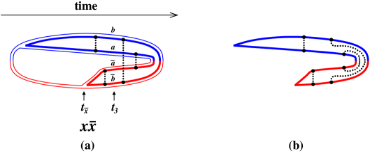
Figure 37: (a) An example of non-trivial color interaction in single splitting after the last emission time $t_{\bar{\rm x}}$. This figure uses a combination of our notation and that of Blaizot et al. Blaizot0 . The high-energy gluons are drawn with the double line notation of large $N_{\rm c}$. Correlations representing interactions with the medium are show as black dotted lines and correspond to the same sorts of correlations as depicted by black double lines in fig. 23. The thick-curve fundamental-representation loop plus the particular example of dotted correlation lines shown is equivalent to fig. 9 of ref. Blaizot0 . The time $t_{3}$ indicated above is the same as the time $t_{3}$ in their figure, and our labels $a,b,\bar{a},\bar{b}$ here correspond to theirs. (b) The same fundamental-representation loop, with the correlations drawn in a topologically equivalent way just to make it clear that this example represents a planar diagram bounded by the loop and so leading order in large $N_{\rm c}$.

In the formalism of Blaizot et al., what happens when we do integrate over final transverse momenta? Integrating over final transverse momenta ${\bm{k}}_{a}$ and ${\bm{k}}_{b}$ in their differential cross-section (3.13) is equivalent, in the transverse position space used in their (4.1), to equating $(\bar{\bm{y}}_{a},\bar{\bm{y}}_{b})=({\bm{y}}_{a},{\bm{y}}_{b})$ and then integrating over $({\bm{y}}_{a},{\bm{y}}_{b})$. In their formula (4.15) for the effects of late-time correlations such as shown in our fig. 37, the factor $({\bm{y}}_{a};\bar{\bm{y}}_{a}|S^{(2)}(t_{L},t_{3})|{\bm{z}}_{a};\bar{\bm{z}}_{a})$ then forces ${\bm{z}}_{a}=\bar{\bm{z}}_{a}$. (Similarly, ${\bm{z}}_{b}=\bar{\bm{z}}_{b}$.) This makes the $T(Z)$ of their (4.16) vanish, which means that their (4.15) vanishes: what they call the “non-factorizable” contributions vanish when integrated over final transverse momenta.

References

- (1) L. D. Landau and I. Pomeranchuk, “Limits of applicability of the theory of bremsstrahlung electrons and pair production at high-energies,” Dokl. Akad. Nauk Ser. Fiz. 92 (1953) 535; “Electron cascade process at very high energies,” ibid. 735.
- (2) A. B. Migdal, “Bremsstrahlung and pair production in condensed media at high-energies,” Phys. Rev. 103, 1811 (1956);
- (3) L. Landau, The Collected Papers of L.D. Landau (Pergamon Press, New York, 1965).
- (4) J. P. Blaizot and Y. Mehtar-Tani, “Renormalization of the jet-quenching parameter,” Nucl. Phys. A 929, 202 (2014) [arXiv:1403.2323 [hep-ph]].
- (5) E. Iancu, “The non-linear evolution of jet quenching,” JHEP 1410, 95 (2014) [arXiv:1403.1996 [hep-ph]].
- (6) B. Wu, “Radiative energy loss and radiative -broadening of high-energy partons in QCD matter,” JHEP 1412, 081 (2014) [arXiv:1408.5459 [hep-ph]].
- (7) P. Arnold and S. Iqbal, “The LPM effect in sequential bremsstrahlung,” JHEP 1504, 070 (2015) [erratum JHEP 1609, 072 (2016)] [arXiv:1501.04964 [hep-ph]].
- (8) K. M. Burke et al. [JET Collaboration], “Extracting the jet transport coefficient from jet quenching in high-energy heavy-ion collisions,” Phys. Rev. C 90, no. 1, 014909 (2014) [arXiv:1312.5003 [nucl-th]].
- (9) M. Gyulassy et al., “Quantitative Jet and Electromagnetic Tomography (JET) of Extreme Phases of Matter in Heavy-ion Collisions,” doi:10.2172/1242882.
- (10) A. Majumder, “Hard Probes: After the dust has settled!,” arXiv:1510.01581 [nucl-th].
- (11) S. Jeon and G. D. Moore, “Energy loss of leading partons in a thermal QCD medium,” Phys. Rev. C 71, 034901 (2005) [arXiv: hep-ph/0309332].
- (12) P. B. Arnold, S. Cantrell and W. Xiao, “Stopping distance for high energy jets in weakly-coupled quark-gluon plasmas,” Phys. Rev. D 81, 045017 (2010) [arXiv:0912.3862 [hep-ph]].
- (13) J. P. Blaizot, E. Iancu and Y. Mehtar-Tani, “Medium-induced QCD cascade: democratic branching and wave turbulence,” Phys. Rev. Lett. 111, 052001 (2013) [arXiv:1301.6102 [hep-ph]].
- (14) J. P. Blaizot and Y. Mehtar-Tani, “Jet Structure in Heavy Ion Collisions,” Int. J. Mod. Phys. E 24, no. 11, 1530012 (2015) [arXiv:1503.05958 [hep-ph]].
- (15) E. W. Kolb and S. Wolfram, “Baryon Number Generation in the Early Universe,” Nucl. Phys. B 172, 224 (1980) [erratum Nucl. Phys. B 195, 542 (1982)].
- (16) K. C. Zapp, J. Stachel and U. A. Wiedemann, “A local Monte Carlo framework for coherent QCD parton energy loss,” JHEP 1107, 118 (2011) [arXiv:1103.6252 [hep-ph]]; K. C. Zapp, F. Krauss and U. A. Wiedemann, “A perturbative framework for jet quenching,” JHEP 1303, 080 (2013) [arXiv:1212.1599 [hep-ph]].
- (17) C. Shen, C. Park, J. F. Paquet, G. S. Denicol, S. Jeon and C. Gale, “Direct photon production and jet energy-loss in small systems,” arXiv:1601.03070 [hep-ph]; Chanwook Park, “Jet energy loss with finite-size effects and running coupling in MARTINI,” MSc thesis, McGill University, 2015 (McGill PID # 139184).
- (18) P. Nason, “A New method for combining NLO QCD with shower Monte Carlo algorithms,” JHEP 0411, 040 (2004) [hep-ph/0409146]; S. Frixione, P. Nason and C. Oleari, “Matching NLO QCD computations with Parton Shower simulations: the POWHEG method,” JHEP 0711, 070 (2007) [arXiv:0709.2092 [hep-ph]].
- (19) M. Fickinger, G. Ovanesyan and I. Vitev, “Angular distributions of higher order splitting functions in the vacuum and in dense QCD matter,” JHEP 1307, 059 (2013) [arXiv:1304.3497 [hep-ph]].
- (20) J. Casalderrey-Solana, D. Pablos and K. Tywoniuk, “Jet formation and interference in a thin QCD medium,” arXiv:1512.07561 [hep-ph].
- (21) P. Arnold, H. C. Chang and S. Iqbal, “The LPM effect in sequential bremsstrahlung: 4-gluon vertices,” to appear in JHEP, arXiv:1608.05718 [hep-ph].
- (22) J. P. Blaizot, F. Dominguez, E. Iancu and Y. Mehtar-Tani, “Medium-induced gluon branching,” JHEP 1301, 143 (2013) [arXiv:1209.4585 [hep-ph]].
- (23) R. Baier, “Jet quenching,” Nucl. Phys. A 715, 209 (2003) [hep-ph/0209038].
- (24) S. Peigne and A. V. Smilga, “Energy losses in a hot plasma revisited,” Phys. Usp. 52, 659 (2009) [Usp. Fiz. Nauk 179, 697 (2009)] [arXiv:0810.5702 [hep-ph]].
- (25) J. F. Gunion and G. Bertsch, “Hadronization By Color Bremsstrahlung,” Phys. Rev. D 25, 746 (1982).
- (26) T. Liou, A. H. Mueller and B. Wu, “Radiative -broadening of high-energy quarks and gluons in QCD matter,” Nucl. Phys. A 916, 102 (2013) [arXiv:1304.7677 [hep-ph]].
- (27) J. P. Blaizot, F. Dominguez, E. Iancu and Y. Mehtar-Tani, “Probabilistic picture for medium-induced jet evolution,” JHEP 1406, 075 (2014) [arXiv:1311.5823 [hep-ph]].
- (28) E. Iancu and D. N. Triantafyllopoulos, “Running coupling effects in the evolution of jet quenching,” Phys. Rev. D 90, 074002 (2014) [arXiv:1405.3525 [hep-ph]].
- (29) P. Arnold, H. C. Chang and S. Iqbal, “The LPM effect in sequential bremsstrahlung: dimensional regularization,” to appear in JHEP, arXiv:1606.08853 [hep-ph].
- (30) Y. Mehtar-Tani, C. A. Salgado and K. Tywoniuk, “The Radiation pattern of a QCD antenna in a dense medium,” JHEP 1210, 197 (2012) [arXiv:1205.5739 [hep-ph]].
- (31) R. Baier, Y. L. Dokshitzer, A. H. Mueller, S. Peigne and D. Schiff, “The Landau-Pomeranchuk-Migdal effect in QED,” Nucl. Phys. B 478, 577 (1996) [arXiv:hep-ph/9604327]; “Radiative energy loss of high-energy quarks and gluons in a finite volume quark - gluon plasma,” ibid. 483, 291 (1997) [arXiv:hep-ph/9607355]; R. Baier, Y. L. Dokshitzer, A. H. Mueller, S. Peigne and D. Schiff, “Radiative energy loss and -broadening of high energy partons in nuclei,” ibid. 484 (1997) [arXiv:hep-ph/9608322].
- (32) B. G. Zakharov, “Fully quantum treatment of the Landau-Pomeranchuk-Migdal effect in QED and QCD,” JETP Lett. 63, 952 (1996) [arXiv:hep-ph/9607440]; “Radiative energy loss of high-energy quarks in finite size nuclear matter an quark - gluon plasma,” ibid. 65, 615 (1997) [Pisma Zh. Eksp. Teor. Fiz. 63, 952 (1996)] [arXiv:hep-ph/9607440].
- (33) P. B. Arnold, “Simple Formula for High-Energy Gluon Bremsstrahlung in a Finite, Expanding Medium,” Phys. Rev. D 79, 065025 (2009) [arXiv:0808.2767 [hep-ph]].