A cautionary note about composite Galactic star formation relations

Abstract

We explore the pitfalls which affect the comparison of the star formation relation for nearby molecular clouds with that for distant compact molecular clumps. We show that both relations behave differently in the ($\Sigma_{\rm gas}$, $\Sigma_{\rm SFR}$) space, where $\Sigma_{\rm gas}$ and $\Sigma_{\rm SFR}$ are, respectively, the gas and star formation rate surface densities, even when the physics of star formation is the same. This is because the star formation relation of nearby clouds relates gas and star surface densities measured locally, that is, within a given interval of gas surface density, or at a given protostar location. We refer to such measurements as local measurements, and the corresponding star formation relation as the local relation. In contrast, the stellar content of a distant molecular clump remains unresolved. Only the mean star formation rate can be obtained from e.g. the clump infrared luminosity. One clump therefore provides one single point to the ($\Sigma_{\rm gas}$, $\Sigma_{\rm SFR}$) space, that is, its mean gas surface density and star formation rate surface density. We refer to this star formation relation as a global relation since it builds on the global properties of molecular clumps. Its definition therefore requires an ensemble of cluster-forming clumps. We show that, although the local and global relations have different slopes, this per se cannot be taken as evidence for a change in the physics of star formation with gas surface density. It therefore appears that great caution should be taken when physically interpreting a composite star formation relation, that is, a relation combining together local and global relations.

1. Introduction

The star formation rate of a galaxy is a crucial driver of its evolution (Fritze-von Alvensleben & Gerhard, 1994). Its dependence on the gas density and/or galaxy type is often embodied by star formation relations, namely, power-law relations between the surface density of the gas, $\Sigma_{\rm gas}$, and the surface density of the star formation rate, $\Sigma_{\rm SFR}$:

$$\Sigma_{\rm SFR}\propto\Sigma_{\rm gas}^{N}\;.$$ (1)

Based on a combined sample of spiral and starburst galaxies, Kennicutt (1998a) derive a super-linear relation ($N\simeq 1.4$; his fig. 6) between the disk-averaged surface densities of the star formation rate ($\Sigma_{\rm SFR}$) and of the total gas mass ($\Sigma_{\rm gas}$), where the latter accounts for the atomic and molecular hydrogen (obtained via H I and CO measurements, respectively). Equation 1 with $N\simeq 1.4$ is often referred to as the Schmidt - Kennicutt law. Schmidt (1959) was the first to postulate a power-law scaling for the neutral hydrogen and Population I stars of the Galactic disc, for which he found $N\simeq 2$. He also suggested that Eq. 1 could be valid for galaxies.

In addition to surface-density measurements, star formation relations can also be defined based on global measurements, i.e. as the total star formation rate as a function of gas mass. In that respect, Gao & Solomon (2004) investigate how the star formation activity of a sample of spiral, luminous and ultraluminous infrared galaxies scales with their total and dense molecular gas contents. They find a super-linear (slope $\simeq 1.4$) relation between the total star formation rate (as traced by the galaxy far-infrared luminosity, $L_{IR}$) and the total molecular gas mass (as traced by CO luminosity, $L_{CO}$), i.e. $L_{IR}\propto L_{CO}^{1.4}$. That is, the slope is reminiscent of that of Kennicutt (1998a). In contrast, the relation between the star formation rate of galaxies and their dense molecular gas mass (as traced by the HCN line luminosity) is linear, i.e. $L_{IR}\propto L_{HCN}$. This direct proportionality between the star formation rate and the dense gas mass thus differs from the Schmidt - Kennicutt relation. According to Gao & Solomon (2004), the linear scaling $L_{IR}\propto L_{HCN}$ stems from the high-mass star-forming sites being the dense regions of giant molecular clouds, rather than their envelopes which are the main CO-emitters. This is the combination of spiral and starburst galaxies in one single sample which yields $N\simeq 1.4$ in the Schmidt - Kennicutt relation and in the $L_{\rm CO}-L_{\rm IR}$ relation of Gao & Solomon (2004). In starburst, luminous and ultraluminous infrared galaxies, the dense gas mass fraction is higher than in spiral galaxies, thereby promoting a higher star formation activity for a given $L_{\rm CO}$ luminosity.

This interpretation has been strengthened by Wu et al. (2005) who find that the linear correlation between $L_{\rm HCN}$ and $L_{\rm IR}$ established by Gao & Solomon (2004) for entire galaxies also holds for individual molecular clumps of the Galactic disk. Following Gao & Solomon (2004), Wu et al. (2005) therefore also argue that the most relevant parameter for the star formation rate is the amount of dense molecular gas traced by HCN emission, that is, gas with a mean density of $\simeq 3\cdot 10^{4}cm^{-3}$. Further support to this picture has been added by Lada et al. (2012) who find that the total star formation rate of nearby molecular clouds is linearly proportional to their dense gas content (see also Lada, Lombardi & Alves, 2010), and that this relation for molecular clouds might extend that already established for galaxies. In fact, regardless of whether one considers their total gas mass or their dense gas mass, nearby clouds do not show any super-linear star formation relation. That is, the data for the nearby clouds (Lada et al., 2012) and for spiral galaxies (Gao & Solomon, 2004) are incompatible with the classical Schmidt - Kennicutt relation. Lada et al. (2012) show that the star formation relation is linear, from individual clouds to entire galaxies, as long as their dense gas fraction is the same.

In addition to the global measurements for galaxies and molecular clouds quoted above, star formation relations have also been established for the interiors of molecular clouds of the Solar neighborhood (e.g., Heiderman et al., 2010; Gutermuth et al., 2011; Lombardi, Lada & Alves, 2013; Lada et al., 2013):

$$\Sigma_{\star}\propto\Sigma_{\rm gas}^{N^{\prime}}\,,$$ (2)

where $\Sigma_{\rm gas}$ and $\Sigma_{\star}$ are the surface densities of gas and young stellar objects (YSOs) measured in a particular region of a molecular cloud, rather than averaged over the entire cloud. The spatial scale of these star formation relations is therefore the pc-scale, and the measured slope ranges from $N^{\prime}\simeq 2$ (Gutermuth et al., 2011; Lombardi, Lada & Alves, 2013; Lada et al., 2013) to $N^{\prime}\simeq 3$ (Heiderman et al., 2010; Lada et al., 2013). By assigning a duration to the star formation episode, $t_{SF}$, one obtains the surface density of the star formation rate:

$$\Sigma_{\rm SFR}=\frac{\Sigma_{\star}}{t_{SF}}\propto\Sigma_{\rm gas}^{N^{\prime}}\,,$$ (3)

an equation analogous to Eq. 1 although, given the local nature of its measurements, Eq. 3 cannot be directly compared to Eq. 1.

Nearby molecular clouds are exquisite targets when it comes to resolving their stellar content on a YSO-by-YSO basis, but they are devoid of massive stars. To learn about massive-star formation, we must look at compact molecular clumps with distances of, typically, several kpc. At such distances, their embedded stellar content remains unresolved (although ALMA is now changing that). Their star formation activity must thus be traced by a global property such as the clump total infrared luminosity, $24\,\mu m$ emission, or radio continuum emission (Vutisalchavakul & Evans, 2013).

Wu et al. (2010) obtain the total ($8-1000\,\mu m$) infrared luminosity, $L_{IR}$, and the mean gas surface density of about 50 molecular clumps of the Galactic disk. In a comprehensive study aimed at comparing the star formation relations of nearby molecular clouds, distant molecular clumps and galaxies, Heiderman et al. (2010) compare the gas and star formation rate surface densities of these clumps to the star formation relation they have derived for molecular clouds of the Solar neighborhood. To obtain the star formation rate surface density of the clumps, they assume the conversion between the total infrared luminosity and star formation rate established for galaxies by Kennicutt (1998b).

They find that the star formation relation for molecular clumps is shallower than that for molecular clouds (see Figure 9 in Heiderman et al., 2010). Also, at gas surface densities of $\Sigma_{\rm gas}\simeq 300\,M_{\odot}\cdot pc^{-2}$, an increase of the clump star formation rate by a factor of 3-to-10 is needed to bring it in agreement with the values obtained for nearby molecular clouds. Heiderman et al. (2010) quote two possibilities to explain this difference: (i) star-forming regions behave differently in the ($\Sigma_{\rm gas}$, $\Sigma_{\rm SFR}$)-space depending on whether they form massive stars (as for distant clumps), or not (as for nearby molecular clouds); (ii) the $L_{IR}-SFR$ calibration of Kennicutt (1998b) requires an upward correction.

In this contribution, we discuss a third reason as to why there is a shift between the star formation relations for distant clumps and nearby clouds. This effect is the following. While the gas and star formation rate surface densities of distant clumps are averaged over the entire clump extent, in nearby clouds, they can be measured at a given location of the cloud. In what follows we will refer these measurements as global and local, respectively. A local meaurement in a nearby cloud can be done at a given extinction level (e.g. Heiderman et al., 2010), or at a given YSO location (e.g. Gutermuth et al., 2011). In that respect, we stress that the term ‘local’ does not refer to the distance of the clouds (although due to the resolving power needed to identify individual YSOs, local measurements have so far been performed in nearby molecular clouds only). We will show that measuring the gas and star surface densities globally or locally inevitably leads to different star formation relations, in terms of both normalization and slope, even when the underlying physics of star formation is the same. Displaying together the local and global star formation relations yields a broken power-law whose composite nature hinders the physical interpretation. In particular, the steepening of the composite slope at low gas surface densities does not constitute an evidence of a star-formation threshold, at least not a threshold defined in a Heaviside manner in the ($\Sigma_{\rm gas}$, $\Sigma_{\rm SFR}$)-space. That local and global measurements lead to distinct star formation relations have already been highlighted by Lada et al. (2013) who show that there is a difference between the local and global star formation relations of nearby molecular clouds. That is, there is a Schmidt relation within molecular clouds, but not between molecular clouds given that Galactic clouds have a similar averaged surface density.

The paper is organized as follows. In Section 2, we show how global and local star formation relations differ from each other. We also show how the mass-radius relation of molecular clumps drives the slope of their global star formation relation. Section 3 compares models and observations of the local relation. In Section 4, we emphasize that the difference in slope between the local and global relations per se does not indicate a change in the physics of star formation with gas surface density. We also discuss the implications in terms of star formation density threshold. In Section 5, we discuss the difficulties inherent to estimating the star formation efficiency per free-fall time from the global and local relations. Finally, we present our conclusions in Section 6.

2. Global vs. Local Star Formation relations

Molecular clumps are individual regions of massive-star and star-cluster formation. Their size is often quantified with the full-width at half-maximum (FWHM) of a given molecular tracer. As an example, Wu et al. (2010) map molecular clumps in the ${\rm HCN}\,\,J=1-0$ transition, and define their radius, $R_{HCN}$, as half the FWHM of the corresponding radial intensity profile, i.e., $R_{HCN}=0.5\,FWHM_{\rm HCN}$. The gas surface density, $\Sigma_{\rm gas}$, is then averaged over a disk of radius $R_{HCN}$:

$$\Sigma_{\rm gas}=\frac{M_{gas}}{\pi R_{HCN}^{2}}\,,$$ (4)

with $M_{gas}$ the gas mass enclosed within the half-peak intensity contour (see Table 11 in Wu et al., 2010).

To estimate the star formation rate, $SFR$, of a clump, Heiderman et al. (2010) use the clump total infrared luminosity, $L_{IR}$ (8-1000 $\mu$m) (see Table 7 in Wu et al., 2010), and assume the conversion of Kennicutt (1998b):

$$SFR_{IR}(M_{\odot}\cdot yr^{-1})\simeq 2\times 10^{-10}L_{IR}(L_{\odot})\;.$$ (5)

Note that this relation was introduced for optically-thick starburst galaxies, whose bolometric stellar luminosity is reprocessed in the infrared. We will further discuss Eq. 5 in section 5.2.

The clump star formation rate surface density, $\Sigma_{\rm SFR_{IR}}$, is also averaged over a disk of radius $R_{HCN}$:

$$\Sigma_{\rm SFR_{IR}}=\frac{\rm SFR_{IR}}{\pi R_{HCN}^{2}}$$ (6)

(see Eq. 16 and Table 6 in Heiderman et al., 2010).

We refer to $\Sigma_{\rm gas}$ and $\Sigma_{\rm SFR_{IR}}$ as global surface densities since they are averaged over the whole FWHM-extent of the clump.

For nearby star-forming regions, however, it is possible to measure the surface densities of gas and YSOs in successive intervals of visual extinction nested inside a given molecular cloud. That is, clouds are divided into contour levels of gas surface density, and the gas mass, YSO number and surface area are measured for each interval (see Fig. 2 in Heiderman et al., 2010). We refer the corresponding surface densities as local surface densities.

The difference in how both measurements are carried out is illustrated in Fig. 1 for the case of a spherical reservoir of gas. It should be noted that in case of global measurements (left panel of Fig. 1), to define a star formation relation requires a population of molecular clumps (since each clump provides one point in the ($\Sigma_{\rm gas}$, $\Sigma_{\rm SFR}$)-space). In case of local measurements (right panel of Fig. 1), a molecular cloud or, even, one only of its embedded clusters, is enough to define a star formation relation. In what follows, we will refer to the star formation relation of Heiderman et al. (2010) as a local relation, and the star formation relation of an ensemble of dense clumps as its global counterpart.

We note that the star formation relations obtained by Gutermuth et al. (2011) for a sample of nearby molecular clouds is also a local relation since the gas and YSO surface densities are measured in the vicinity of each YSO based on a nearest-neighbor scheme.

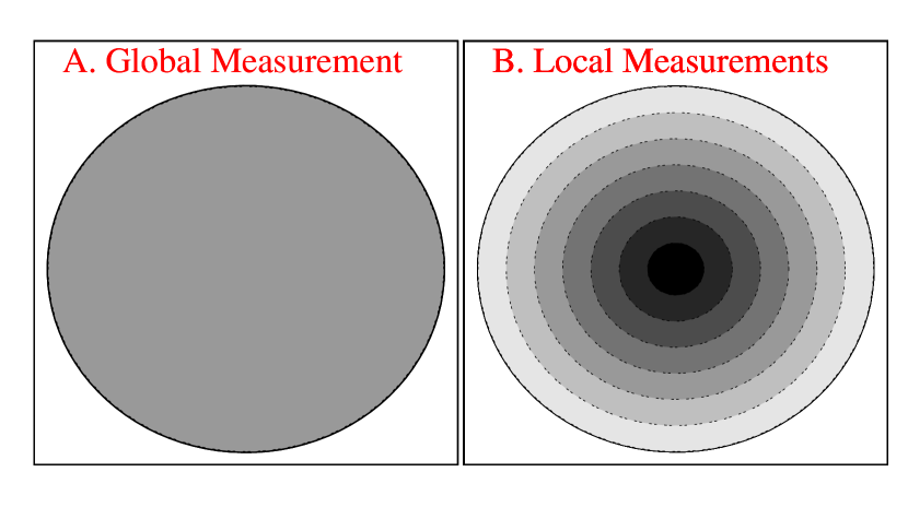
Figure 1.— Illustration of global and local measures of surface densities. In a global measure (left panel), the surface densities of the gas and stars (or of the star formation rate) are averaged over the whole molecular clump. In a local measure (right panel), the surface densities are averaged within given contour intervals of the gas surface density. Whether the surface densities are measured locally or globally leads to different star formation relations (see Section 2).

In the next section, we build on the concept of star formation efficiency per free-fall time to obtain the global star formation relation of molecular clumps as a function of their mass-radius relation. We will assume that the star formation efficiency per free-fall time is a constant. This seems to be a reasonable hypothesis on the spatial scale of a forming-cluster (i.e. a few pc) since the slope of the local relation predicted by the model of Parmentier & Pfalzner (2013) ($N^{\prime}\simeq 2$) matches the observed one (Gutermuth et al., 2011; Lombardi, Lada & Alves, 2013; Lada et al., 2013) when the star formation efficiency per free-fall time is constant. If it were to increase with gas density, the local star formation relation would be steeper, a possibility we discuss in Section 3.

2.1. The Global Star Formation Relation

Consider a molecular clump with a gas mass $M_{g}$ enclosed within a radius $R$. Here, we remind that molecular clumps lack a neat outer boundary. Their radius is often defined as half the FWHM of a given gas-tracer, with the clump mass the gas mass enclosed inside the half-peak intensity contour. The mean surface densities of the gas and star formation rate of the clump are, respectively:

$$\Sigma_{\rm gas}^{glob}(t)=\frac{M_{g}(t)}{\pi R^{2}}$$ (7)

and

$$\Sigma_{\rm SFR}^{glob}(t)=\frac{{\rm SFR}(t)}{\pi R^{2}}\,,$$ (8)

where $t$ is the time elapsed since the onset of star formation. We assume that a clump is an isolated system (i.e. no inflows or outflows) and that it is in static equilibrium. As a result, the surface densities of the gas and star formation rate decrease with time as a result of gas-feeding to star formation (see Parmentier, Pfalzner & Grebel, 2014, for a discussion about the evolution of the star formation rate).

The global star formation rate of the clump obeys:

$$SFR(t)\simeq\epsilon_{\rm ff}\frac{M_{g}(t)}{\tau_{\rm ff}(t)}\,,$$ (9)

with $\epsilon_{\rm ff}$ the star formation efficiency per free-fall time and $M_{g}(t)$ the gas mass not yet processed into stars at time $t$. $\tau_{\rm ff}$ is the free-fall time at the mean volume density of the clump gas, i.e.:

$$\tau_{\rm ff}(t)=\sqrt{\frac{3\pi}{32G\rho_{g}(t)}}\,,$$ (10)

with $\rho_{g}(t)=3M_{g}(t)/(4\pi R^{3})$ and $G$ the gravitational constant. As we shall see later, Equation (9) slightly underestimates the actual star formation rate of centrally-concentrated molecular clumps.

The surface density of the clump star formation rate is then simply:

$$\Sigma_{SFR}^{glob}(t)=\frac{SFR(t)}{\pi R^{2}}=\frac{\epsilon_{\rm ff}}{\tau_{\rm ff}(t)}\cdot\frac{M_{g}(t)}{\pi R^{2}}=\frac{\epsilon_{\rm ff}}{\tau_{\rm ff}(t)}\cdot\Sigma_{\rm gas}^{glob}(t)\;.$$ (11)

To define a star formation relation based on Eq. 11, one needs to consider an ensemble of molecular clumps. Let us first consider clumps with a common mean volume density and, therefore, the same free-fall time. Equation 11 shows that, with $\epsilon_{\rm ff}$/$\tau_{\rm ff}$ a constant among the clump population, the slope of the global star formation relation is unity ($N=1$). Its normalization depends on the clump volume density and on the star formation efficiency per free-fall time. The denser the clump and/or the higher the star formation efficiency per free-fall time, the higher the star formation rate surface density. [We will look into the time evolution later in this section]

Now let us consider a population of clumps with identical radii, rather than identical volume densities. Equation (11) can be rewritten as:

$$\Sigma_{SFR}^{glob}(t)=2\epsilon_{\rm ff}\sqrt{\frac{2G}{\pi R}}\cdot[\Sigma_{g}(t)]^{3/2}\;.$$ (12)

The star formation relation is now steeper ($N=1.5$) than found for a common mean volume density ($N=1$). That is, the slope of the global star formation relation depends on the assumed clump mass-radius relation. At constant radius, the volume density of the gas increases along with its surface density, which speeds up star formation as $\Sigma_{\rm gas}$ increases.

If the star-forming molecular clumps are characterized by a common mean surface density, then the star formation relation becomes a vertical in the ($\Sigma_{\rm gas}$, $\Sigma_{\rm SFR}$) space. The same pattern holds for giant molecular clouds, given their common mean surface density, as already highlighted by Lada et al. (2013) (see their fig. 8). We therefore note that to define a global star formation relation for molecular clumps is an ambiguous task, as the slope depends on the clump mass-radius relation.

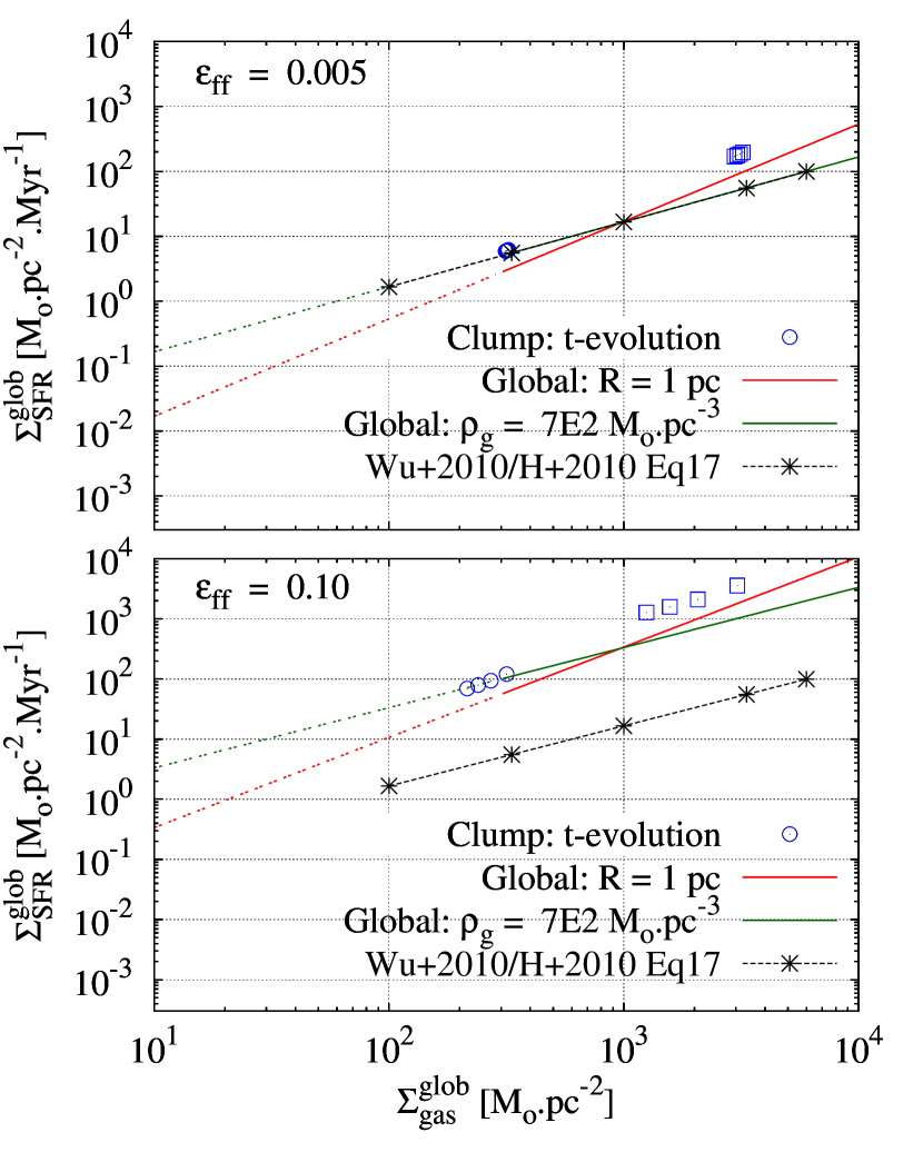
Figure 2.— Global star formation relations for two populations of molecular clumps, one with a given mean volume density of 700$M_{\odot}\cdot pc^{-3}$ (Eq. 11, green line) and one with a given radius of 1 pc (Eq. 12, red line). The black line with asterisks is Equation 17 of Heiderman et al. (2010), which shows the region of the diagram where the clumps mapped in HCN 1-0 by Wu et al. (2010) are located. The blue open symbols show how the surface densities evolve with time for clumps with a radius of 1 pc, and masses of $10^{3}M_{\odot}$ (circles) and $10^{4}M_{\odot}$ (squares). The time-evolution is from right to left and the displayed time-span is 2 Myr. The star formation efficiency per free-fall time is $\epsilon_{\rm ff}=0.005$ and $\epsilon_{\rm ff}=0.10$ in the top and bottom panels, respectively (see Section 2.1 for details).

Equations (11) and (12) are shown in both panels of Fig. 2 as the green and red lines, respectively. Equation (11) uses a free-fall time of 0.3 Myr, which corresponds to a mean volume density of $700\,M_{\odot}\cdot pc^{-3}$, or a number density of $n_{H2}\simeq 10^{4}\,cm^{-3}$. This is the median number density of the clumps mapped in HCN 1-0 by Wu et al. (2010). An order of magnitude for the radius of these clumps is 1 pc, and we therefore adopt $R=1\,pc$ in Equation (12).

In the top panel of Fig. 2, a star formation efficiency per free-fall time of $\epsilon_{\rm ff}=0.005$ is adopted so that Equation (11) (the green line) matches Equation 17 of Heiderman et al. (2010) (black line with asterisks). That equation, which we reproduce here for the sake of clarity,

$$\Sigma_{\rm SFR}\simeq 1.66\times 10^{-2}\left(\frac{\Sigma_{{\rm HCN}(1-0)}}{1M_{\odot}\cdot pc^{-2}}\right)(M_{\odot}\cdot Myr^{-1}\cdot pc^{-2})\,,$$ (13)

provides a good match to the locus of the HCN 1-0 clumps of Wu et al. (2010) (see also the middle panel of Fig. 5 where Eq. 17 of Heiderman et al. (2010) is shown along with the data of Wu et al. (2010)).

In the bottom panel of Fig.  2, the star formation efficiency per free-fall time is $\epsilon_{\rm ff}=0.10$, which increases the intercept of Eqs 11 and 12 by a factor of 20 compared to the top panel. $\epsilon_{\rm ff}=0.10$ is the star formation efficiency per free-fall time used by Parmentier & Pfalzner (2013) to match their model onto the observed local star formation relation of Gutermuth et al. (2011).

It is puzzling that there is such a difference in the star formation efficiency per free-fall time needed to match the global surface densities of distant dense clumps on the one hand (top panel), and the local surface densities of nearby clouds on the other (see fig. 3 in Parmentier & Pfalzner, 2013). The discrepancy may stem from either observed clump stellar surface densities being underestimated, or observed cloud stellar surface densities being overestimated, or a combination of both. We will further discuss this issue in Section 5.

The blue open circles and squares indicate how an isolated clump in static equilibrium evolves with time in the ($\Sigma_{\rm gas}^{glob}$, $\Sigma_{\rm SFR}^{glob}$) parameter space according to the semi-analytical model of Parmentier & Pfalzner (2013). In Fig. 2, the star formation rate of these model clumps is averaged over time. That is, it is defined as the total stellar mass built at time $t$, $M_{\star}^{glob}(t)$, divided by $t$. The star formation rate surface density thus obeys:

$$\Sigma_{SFR}^{glob}(t)=\frac{M_{\star}^{glob}(t)}{\pi R^{2}\cdot t}=\frac{\Sigma_{\star}^{glob}(t)}{t}\;.$$ (14)

As part of the gas is used for star formation, the star formation efficiency per free-fall time is applied to an ever lower gas mass over an ever longer free-fall time. As a result, the clump location moves toward smaller surface densities of both the gas and star formation rate. The adopted clump radius is 1 pc, the initial gas masses are $10^{3}M_{\odot}$ (circles) and $10^{4}M_{\odot}$ (squares), and the physical time-span is 2 Myr.

As expected, the amount of evolution is larger for higher $\epsilon_{\rm ff}$ and/or higher densities. That is, the span in surface densities is larger in the bottom panel ($\epsilon_{\rm ff}=0.10$) than in the top panel ($\epsilon_{\rm ff}=0.005$), and is also larger for the squares than for the circles. The length of the sequence also depends on the adopted time-span. Here it is assumed that cluster-forming clumps retain their gas during at least 2 Myr. This time-span remains uncertain, however. The time-scale needed for an embedded cluster to expel its residual star-forming gas depends on an array of parameters, ranging from the depth of the forming-cluster gravitational potential (hence the clump mass and radius; Parmentier et al., 2008), to the kinetic energy released into the intra-cluster medium by the newly formed massive stars (Dib et al., 2011). The kinetic energy itself depends on the clump mass, star formation efficiency, the stellar initial mass function and how-well it is sampled in the high-mass regime. Another factor at work is the duration of the pre-main sequence phase as a function of stellar mass. Star-forming regions of the Solar neighborhood contains Class II and Class III YSOs. Given that the life-time of a Class II object is $\simeq 2$ Myr (Evans et al., 2009), this means that these regions have been experiencing star formation for at least 2 Myr (but see Bell et al., 2013, for a longer estimate). Dense and massive molecular clumps, however, contain intermediate-mass and massive pre-main-sequence stars which settle on the main sequence within significantly less than 2 Myr. Stellar winds, and stellar feedback in general, may thus terminate the cluster embedded stage at an earlier time than in the Solar neighborhood. Our adopted time-span of 2 Myr may thus be an upper limit in the case of dense and massive clumps, as may be the length of the sequence of blue open symbols in Fig. 2.

Given that the model clump radius is 1 pc, one would expect to find the starting point of each blue sequence on the red line, which depicts the global star formation relation for a population of clumps with $R=$1 pc (Equation 12). The shift between the red lines and the blue-sequence starting points arises because the latter accounts for the concentrated nature of molecular clumps. Star formation proceeds faster in clumps with volume-density gradients than in clumps with a flat density profile. The initial gas volume density profile adopted for the open blue symbols of Fig. 2 is an isothermal sphere (i.e. $\rho_{gas}(r,t=0)\propto r^{-2}$ with $r$ the distance to the clump center). For such a density profile, the global star formation efficiency achieved within one free-fall time is not $\epsilon_{\rm ff}$, as may be naively expected, but $1.6\epsilon_{\rm ff}$ (see Parmentier, 2014). The clump density profile cannot be taken into account by the simple Eq. 9, from which Equation 12 is derived. Shifting upwards the analytical solution given by Equation 12 (red line) by a factor 1.6 brings it in agreement with the numerical solution illustrated by the blue open symbols.

A point worth being emphasized in this section is that even if star formation operates on a given star formation efficiency per free-fall time, the slope of the star formation relation is not necessarily $N=1.5$. The Kennicutt-Schmidt relation (for galaxies) has an index $N=1.4$ (Kennicutt, 1998a). This is often taken as an evidence that star formation proceeds with a given star formation efficiency per free-fall time since the star formation rate then scales as the gas mass divided by the gas free-fall time (Eq. 9). Expressed in terms of the volume densities of gas, $\rho_{gas}$, and star formation rate, $\rho_{SFR}$, this gives:

$$\rho_{SFR}\propto\frac{\rho_{gas}}{(G\rho_{gas})^{-0.5}}\propto(\rho_{gas})^{1.5}\,,$$ (15)

and, if the gas scale-height does not vary strongly from galaxy-to-galaxy:

$$\Sigma_{SFR}\propto(\Sigma_{gas})^{1.5}\,,$$ (16)

in agreement with the observed Kennicutt-Schmidt relation (see e.g. Wong & Blitz, 2002; Krumholz & Thompson, 2007).

This line-of-reasoning, however, implies that the star formation relation spans a range of volume densities. As we have seen above, when considering star-forming units with a limited range of mean volume densities (e.g. clumps mapped in HCN $J=1-0$), the star formation relation is as given by Eq. 11 with $\tau_{\rm ff}$ roughly constant and, thus, $N=1$. Therefore, an observed global star formation relation with $N\neq 1.5$ does not necessarily disprove the hypothesis that star formation proceeds with a given star formation efficiency per free-fall time.

2.2. The Local Star Formation Relation

Having dealt with the global properties of clumps, we next investigate how the stars and gas are distributed inside them. That is, for a given clump, we now focus on the radial profiles of the gas and star surface densities, $\Sigma_{\rm gas}^{loc}(s,t)$ and $\Sigma_{\star}^{loc}(s,t)$, and we obtain the corresponding star formation relation. $t$ is the time elapsed since the onset of star formation, and $s$ is the projected distance from the clump center (while we denote $r$ its three-dimensional counterpart). The clump can be a compact high-density one, or a larger and more diffuse one (e.g. a concentration of embedded YSOs in a nearby molecular cloud). Spherical symmetry is assumed in any case.

To obtain $\Sigma_{\star}^{loc}(s,t)$ and $\Sigma_{\rm gas}^{loc}(s,t)$, we build on the model of Parmentier & Pfalzner (2013) which predicts the star formation history of isolated spheres of gas in static equilibrium. The principle of this model is to associate a given star formation efficiency per free-fall time, $\epsilon_{\rm ff}$, to an initial gas density profile, $\rho_{0}(r)$. The volume density profile of the gas not yet turned into stars at time $t$, $\rho_{g}(t,r)$, and the volume density profile of the forming cluster, $\rho_{\star}(t,r)$, are given by Equations (19) and (20) in Parmentier & Pfalzner (2013), respectively. We reproduce them below for the sake of clarity:

$$\rho_{g}(r,t)=\left(\rho_{0}(r)^{-1/2}+\sqrt{\frac{8G}{3\pi}}\cdot\epsilon_{\rm ff}\cdot t\right)^{-2}\,,$$ (17)

and

$$\rho_{\star}(r,t)=\rho_{0}(r)-\left(\rho_{0}(r)^{-1/2}+\sqrt{\frac{8G}{3\pi}}\cdot\epsilon_{\rm ff}\cdot t\right)^{-2}\;.$$ (18)

We emphasize that the model is purely volumetric, i.e. the star formation efficiency per free-fall time is applied to the volume density, with the conversion to surface density being performed for the sole purpose of comparing the model to observations. The projection in two dimensions of Equations (17)-(18) provides the relation between $\Sigma_{\star}^{loc}(s,t)$ and $\Sigma_{\rm gas}^{loc}(s,t)$ (see Fig. 3 in Parmentier & Pfalzner, 2013). This is the local star formation relation, that is, the star formation relation defined all through a clump, as opposed to the global star formation relation defined for a population of clumps.

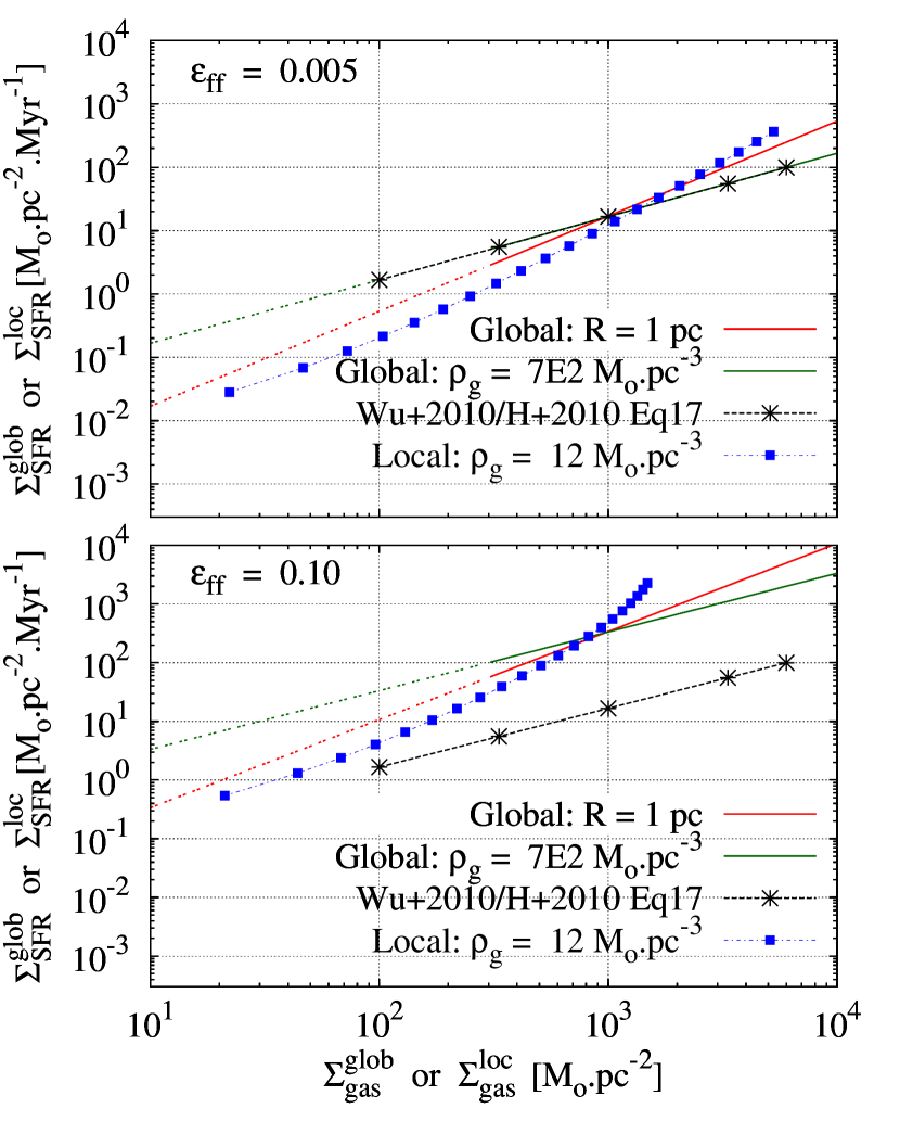
Figure 3.— Same as Figure 2, but completed with the local star formation relation for a molecular clump of radius 6 pc and total mass $10^{4}\,M_{\odot}$ (blue line with plain squares).

At this stage, we still need to obtain the surface density of the star formation rate. We therefore divide $\Sigma_{\star}^{loc}(s,t)$ by the time-span $t$ since star formation onset so as to convert the local surface density in YSOs, $\Sigma_{\star}^{loc}(s,t)$, into the local surface density of the star formation rate, $\Sigma_{\rm SFR}^{loc}(s,t)$:

$$\Sigma_{\rm SFR}^{loc}(s,t)=\frac{\Sigma_{\star}^{loc}(s,t)}{t}\;.$$ (19)

We note that Eq. 19 does not define an instantaneous value, but a time-averaged one. This is the star formation rate surface density which would be inferred by observers based on the YSO number, YSO mean mass, star formation duration, and the cloud surface area where YSOs have been counted. An estimate of the instantaneous star formation rate surface density can be obtained based on the number of protostars and duration of the Class 0+Class I phases (Heiderman et al., 2010; Lada et al., 2013).

How $\Sigma_{\rm gas}^{loc}(s,t)$ and $\Sigma_{\rm SFR}^{loc}(s,t)$ relate to each other is shown in Fig. 3 as the (blue) line with plain squares. The model star-forming region is a clump with a radius of 6 pc and a total mass of $10^{4}\,M_{\odot}$, thus a mean volume density of $12\,M_{\odot}\cdot pc^{-3}$. This is about 60 times less dense than the median HCN 1-0 clump of Wu et al. (2010). This low-density star-forming region is representative of the highest concentration of YSOs in the MonR2 molecular cloud, one of the nearby clouds surveyed by Gutermuth et al. (2011). $t=2$ Myr is adopted and the initial gas density profile is an isothermal sphere. The top and bottom panels of Fig. 3 are identical to those of Fig. 2 except that the open symbols (time evolution of high-density clumps) have been removed for the sake of clarity. Figure 3 shows clearly that the global and local star formation relations have different slopes. The local relation has a slope of about two ($N^{\prime}\simeq 2$; Gutermuth et al., 2011; Parmentier & Pfalzner, 2013), which is steeper than the global star formation relations given by Equations 11 ($N=1$) and 12 ($N=1.5$).

2.3. Global vs. Local

We can now understand the issues set in the introduction. That is, why the observations of Wu et al. (2010) and Heiderman et al. (2010) have different slopes, and why, at a given gas surface density, they do not necessarily provide the same star formation rate surface density. This may simply be the result of the intrinsic differences between the global and local star formation relations, with the former represented by the dense-clump data of Wu et al. (2010), and the latter by the nearby-cloud data of Heiderman et al. (2010). As already stated by Heiderman et al. (2010), this is not necessarily the result of star formation depending on the presence of massive stars. We also note that, at this stage, this does not necessarily call for a change in the calibration between the star formation rate and infrared luminosity of molecular clumps (Eq. 5). Even for a given physics of star formation – e.g. volume-density driven star formation with a given star formation efficiency per free-fall time –, different slopes and different normalizations are expected when measuring the surface densities locally or globally (see Fig. 3). For instance, when $\epsilon_{\rm ff}=0.005$ (top panel of Figure 3), the global star formation relation at constant mean volume density (green line) predicts a star formation rate surface density five times smaller than its local counterpart (blue line with plain squares) at $\Sigma_{\rm gas}\simeq 5000M_{\odot}\cdot pc^{-2}$. It is therefore worth emphasizing that fitting locally-obtained data with a global model could result in the erroneous conclusion that the star formation efficiency per free-fall time is an increasing function of the gas surface density.

Our result that the local and global star formation relations have different slopes is reminiscent of that of Lada et al. (2013). They note that nearby molecular clouds present a power-law local star formation relation (with a slope of 2), but no global star formation relation given that their mean surface density is about constant, at $\Sigma_{gas}\simeq 40\,M_{\odot}\cdot pc^{-2}$. Lada et al. (2013) therefore argue against the classical Schmidt-Kennicutt law (i.e. Eq. 1), which extends down to $\simeq 1\,M_{\odot}\cdot pc^{-2}$, representing a physical relation between the star formation rate and a physical property of the cloud gas. Instead, it results from the unresolved measurements of giant molecular clouds in the disks of galaxies, and from the corresponding beam dilution of the CO observations (see Lada et al., 2013, for a discussion).

3. On the slope of the local star formation relation

Parmentier & Pfalzner (2013) model the relation between the local surface densities in gas and YSOs by applying a constant star formation efficiency per free-fall time to a centrally-concentrated gas sphere. They find a slope steeper than unity, which reflects the fact that the volume density profile of the forming cluster is steeper than that of the gas (their Figs. 1 and 3). The model slope is $N^{\prime}\simeq 2$, in good agreement with the averaged star formation relation found by Gutermuth et al. (2011) for a sample of molecular clouds of the Solar neighborhood. We remind it here for the sake of clarity:

$$\frac{\Sigma_{\star}}{1M_{\odot}\cdot pc^{-2}}\simeq 10^{-3}\frac{\Sigma_{\rm gas}^{2}}{1M_{\odot}\cdot pc^{-2}}\;.$$ (20)

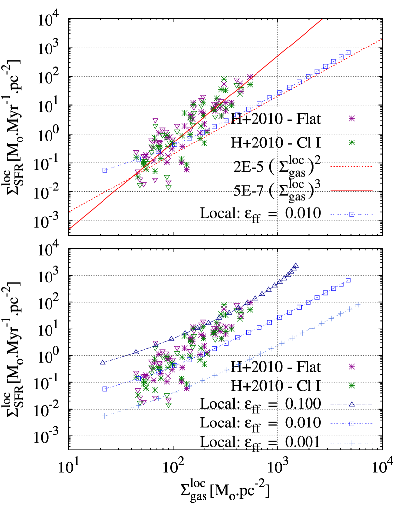
Figure 4.— Top panel: The asterisks and inverted triangles represent the observed local star formation relation of Heiderman et al. (2010) (with symbol- and color-codings similar to their Fig. 9; green and indigo symbols depict Class I and Flat SED YSOs). The two (red) symbol-free straightlines have slopes of two and three, respectively. The (blue) line with open squares shows the model star formation relation for a constant star formation efficiency per free-fall time ($\epsilon_{\rm ff}=0.01$) applied to a sphere of gas with a mass of $10^{4}M_{\odot}$, a radius of 6 pc and a power-law initial gas density profile with a slope of $-2$. While the data follow a slope of about three, the model with a constant $\epsilon_{\rm ff}$ has a slope of two. Bottom panel: data of Heiderman et al. (2010) shown along with three models, each with its own star formation efficiency per free-fall time, from $\epsilon_{\rm ff}=10^{-3}$ (bottom line with plus-signs) up to $\epsilon_{\rm ff}=10^{-1}$ (top line with open triangles).

The data of Heiderman et al. (2010), shown in Figure 4 (color- and symbol-codings similar to their Figure 9), reveal a different picture, however. The top panel shows that these data follow a local star formation relation with a slope of $N^{\prime}\simeq 3$, rather than $N^{\prime}\simeq 2$. That is, the observations are steeper than the prediction for a constant star formation efficiency per free-fall time (shown as the blue line with open squares). We point out that, in Figure 4, both the observations and the model describe a local star formation relation. Therefore, the mismatch between both slopes cannot be ascribed to an inconsistent comparison between a global model and local observations, or vice-versa.

Here, we speculate about two possibilities which may explain this slope difference.

(i) The observations of Heiderman et al. (2010) may suggest that the star formation efficiency per free-fall time increases with the gas density. This is illustrated in the bottom panel of Figure 4, where three models with distinct star formation efficiencies per free-fall time are shown along with the observations.

An increase with gas density of the star formation efficiency per free-fall time would hasten star formation in the clump inner regions. In turn, this would yield a star formation relation steeper than $N^{\prime}\simeq 2$, although it remains to be seen whether this effect is strong enough to explain the observations of Heiderman et al. (2010). Additional consequences would include density profiles of forming clusters steeper than what is predicted by the model of Parmentier & Pfalzner (2013) (see their figs 1 and 2) and, presumably, a greater ability of their inner regions to survive the expulsion of the residual star formation gas. We stress, however, that a proper calibration of the star formation efficiency per free-fall time requires additional parameters such as the mass and volume density of the star-forming region (the cloud mass and radius adopted here are $10^{4}\,M_{\odot}$ and 6 pc, as in Section 2.2). In addition, the data of Heiderman et al. (2010) describe entire molecular clouds, i.e. complexes of cluster-forming clumps. Ideally, one would like to have the data as per molecular clump and to match them with models of the same mass and radius. Therefore, the simple exercise of the bottom panel of Fig. 4 alone does not allow one to quantify the range of $\epsilon_{\rm ff}$ at work in nearby molecular clouds, assuming there is one. It should also be noted that the star formation relation inferred by Gutermuth et al. (2011) presents a range of slopes, from 1.9 (Ophiuchus molecular cloud) to 2.7 (MonR2 molecular cloud), with Eq. 20 providing only a mean trend for their whole cloud sample. The slope and universality of the local star formation relation for molecular clouds of the Solar neighborhood remain therefore debated.

(ii) Lombardi, Lada & Alves (2013) derive, based on a likelihood analysis, a slope of $N^{\prime}\simeq 2$ for the Orion-A molecular cloud (note that their $\beta$-parameter is our $N^{\prime}$ slope). This is in agreement with the model prediction for a constant star formation efficiency per free-fall time. They also generate a synthetic population of protostars obeying a given star formation relation, and investigate how well it is recovered, using either a likelihood analysis or a simple least-squares fit of binned data. Interestingly, the slope they recover with the least-squares fit is significantly steeper than the intrinsic one. For an input/intrinsic slope of $\beta=1.8$, the recovered one is steeper by almost one dex, i.e. $\beta\simeq 2.7$. A maximum-likelihood analysis is needed to recover the input slope accurately. They ascribe the poor accuracy of the standard fit to its inability to account for the Poisson statistics of the bins, and to the loss of information inherent to data binning. Given that the data of Heiderman et al. (2010) correspond to bins in visual extinction, hence gas surface density, it would be interesting to see whether there is a statistical bias responsible for their fairly steep slope of $N^{\prime}\simeq 3$. Such an investigation is beyond the scope of this contribution, however.

An observed local star formation relation steeper than $N^{\prime}\simeq 2$ can therefore result from either a statistical bias, or variations of the star formation efficiency per free-fall time with the gas density (or from any other so far overlooked parameter). This example demonstrates the need and importance of a reliable processing of the data before interpreting them physically.

4. From global to local: On the interpretation of the slope change

4.1. A composite star formation relation

That the local star formation relation is steeper than its global counterpart (see Fig. 3) can lead to the erroneous conclusion that star formation becomes less efficient at gas surface densities lower than the ‘break-point’, that is, the point where both relations cross. This is illustrated in the top panel of Fig. 5 where the adopted models are as in the bottom panel of Fig. 3, that is, a low-density clump (mean volume density of 12 $M_{\odot}\cdot pc^{-3}$) for the local relation, and an ensemble of high-density clumps (mean volume density of 700 $M_{\odot}\cdot pc^{-3}$) for the global relation. In both cases, the star formation efficiency per free-fall time is $\epsilon_{\rm ff}=0.10$. At a gas surface density of $\Sigma_{\rm gas}=\Sigma_{cross}\simeq 600M_{\odot}\cdot pc^{-2}$, the local relation (blue line with plain squares) crosses the global one (green line).

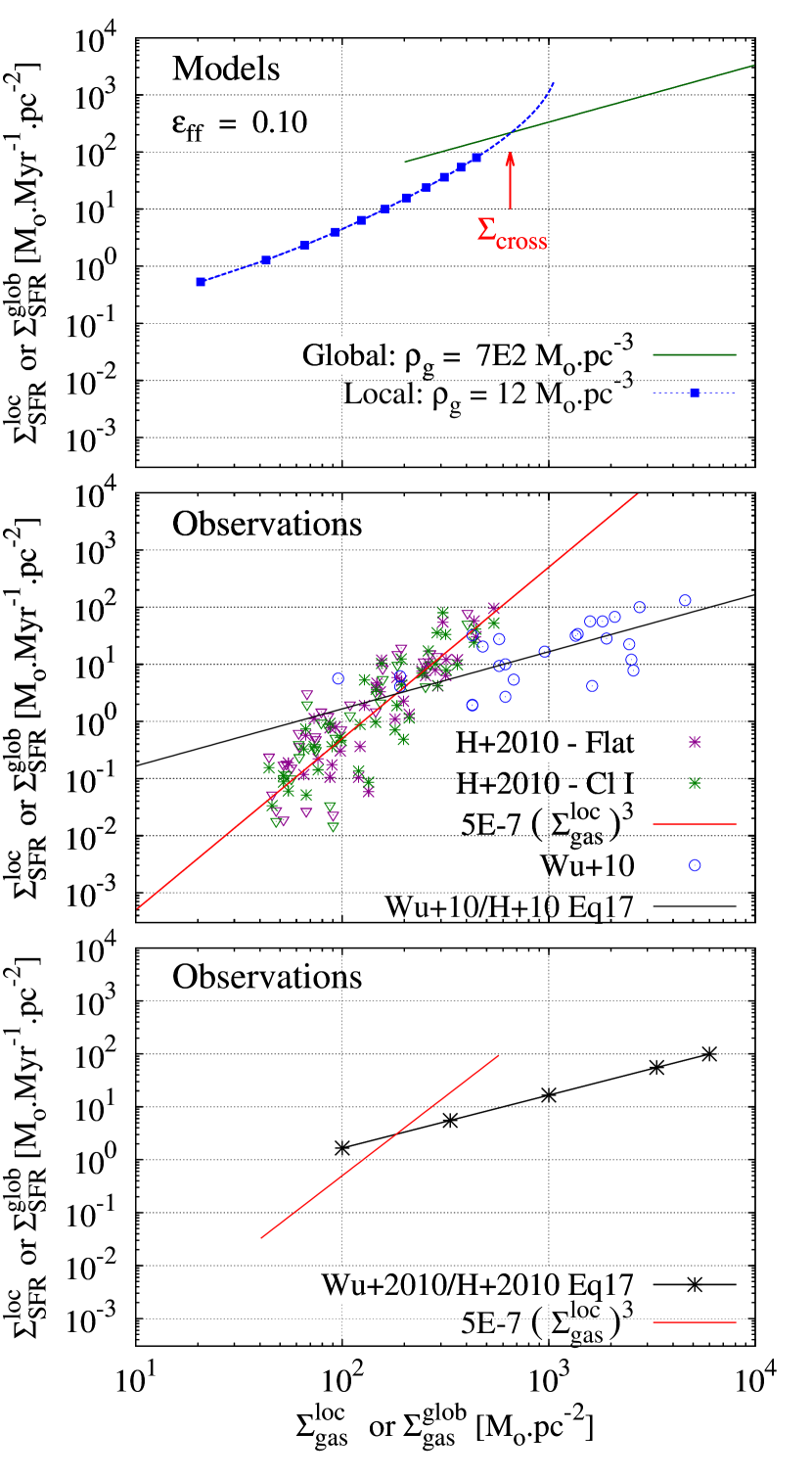
Figure 5.— Top panel: Model local and global relations for the mean volume densities quoted in the key. The vertical arrow indicates the gas surface density, $\Sigma_{cross}$, at which the two star formation relations cross each other. Middle panel: data of Heiderman et al. (2010) for a sample of nearby molecular clouds along with the data of Wu et al. (2010) for a sample of distant molecular clumps. The blue open circles and the black line define a global star formation relation, while the asterisks/inverted triangles and the red line define a local relation. Bottom panel: locus of the two data sets are shown so as to highlight that the change of slope in the star formation relation around $\Sigma_{\rm gas}\simeq 200\,M_{\odot}\cdot pc^{-2}$ stems from swapping a local quantification of star formation for a global one.

An observed local relation is expected to present an upper limit caused by the inability of the observing facility to resolve regions of too high stellar densities. The highest surface density of the star formation rate in Heiderman et al. (2010) is $\Sigma_{SFR,lim}\simeq 100\,M_{\odot}\cdot pc^{-2}\cdot Myr^{-1}$. Model surface densities higher than that limit are represented as a (blue) symbol-free dashed line in the top panel of Fig. 5. As for the observed global relation, it presents a lower limit due to the scarcity of HCN 1-0 clumps whose surface density is lower than $\Sigma_{gas,lim}\simeq 200\,M_{\odot}\cdot pc^{-2}$. We impose the corresponding lower limit to the global relation (solid green line). The combination of both aspects, namely, the change of slope from the global relation to the local one, and their respective ranges in gas and star surface densities, may at first glance suggest that star formation becomes less efficient at $\Sigma_{\rm gas}<\Sigma_{cross}$. Yet, as we have seen, this conclusion would be erroneous. The change in slope stems from modifying how the gas and star surface densities are measured, that is, through a succession of shells in the local relation, while it is averaged over the whole clump extent in the global relation (see Fig. 1). If, additionally, the observed local relation is artificially steepened, as described by Lombardi, Lada & Alves (2013), then the impression of star formation becoming less efficient towards lower gas surface densities is strengthened even more.

The middle panel of Fig. 5 shows the data of Heiderman et al. (2010) (local relation) and of Wu et al. (2010) (global relation). Their respective slopes are $\simeq 3$ (red line) and $\simeq 1$ (black line; Eq. 17 in Heiderman et al. (2010) reproduced as Eq. 13 in this paper). The locus of the observations is further sketched in the bottom panel of Fig. 5 for the sake of clarity, where the broken power-law of the composite star formation relation is clearly highlighted.

The top (models) and bottom (locus of the observations) panels of Fig. 5 present a similar pattern, that is, an apparent decrease in star formation activity below a break-point. This decrease is apparent only: it is driven by the swap of the global star formation relation for a local one towards lower gas surface densities. This also explains why a double power-law yields a better fit to the combined data set of the middle panel than does a single power-law (see section 3.2.1 in Heiderman et al., 2010). We remind again that in the top panel of Fig. 5, the underlying physics of star formation is the same in both the local and global relations. That is, the change of slope from the global relation to the local one does not per se indicate that star formation becomes less efficient with decreasing gas surface density.

We note that the models and observations occupy different locii in the ($\Sigma_{\rm gas}$, $\Sigma_{\rm SFR}$) parameter space, an aspect we will discuss in section 5.

4.2. A threshold for star formation?

Heiderman et al. (2010) observe in their data a steep decline in $\Sigma_{\rm SFR}$ and $\Sigma_{\rm SFR}/\Sigma_{\rm gas}$ at a gas surface density of $\simeq 100-200M_{\odot}\cdot pc^{-2}$. They identify that steep decline as a star formation threshold in gas surface density. While their local measurements alone may already suggest a slope change, the effect is strengthened by the combination of the local and global star formation relations all-together. As we saw in Section 4.1, this leads to a composite star formation relation whose physical interpretation can be spurious.

In the disk of our Galaxy, observational evidence of a Heaviside threshold for star formation in the ($\Sigma_{\rm gas}$, $\Sigma_{\rm SFR}$) space remains ambiguous. Gutermuth et al. (2011) detect none in their local measurements of nearby molecular clouds, consistent with the result of Lada et al. (2013) for the Orion A and Taurus clouds. However, two other clouds in the sample of Lada et al. (2013), Orion B and California, show evidence for such a threshold, the result for Orion B being somewhat less constrained than for California (see eq. 3 and table 1 in Lada et al., 2013).

Although there is no clearly-established Heaviside threshold in the ($\Sigma_{\rm gas}$, $\Sigma_{\rm SFR}$) space, Lada et al. (2013) find evidence for a threshold in the cumulative protostellar fraction, that is, in the evolution of the number of protostars enclosed within a given extinction level as a function of extinction. In the case of Orion A, the bulk of star formation is confined to the high ($\Sigma_{gas}\gtrsim 160M_{\odot}\cdot pc^{-2}$) column-density regions of the cloud. Despite the similar values of the surface density threshold of Heiderman et al. (2010) and Lada et al. (2013), it is important to underline their different physical natures. That is, a threshold in the cumulative protostellar fraction does not equate with a threshold in the local star formation relation. This is best understood by comparing the left and right panels of fig. 5 in Lada et al. (2013). They depict, respectively, the local star formation relation and the variation of the cumulative protostellar fraction with extinction of the Orion A molecular cloud. The star formation threshold identified in their right panel at $\Sigma_{gas}\simeq 160M_{\odot}\cdot pc^{-2}$ ($A_{K}\simeq 0.8\,mag$) does not translate into a threshold in the left panel. It should be noted that no star formation threshold is required by the model of Parmentier & Pfalzner (2013), with the exception of the minimum gas surface density required for the phase transition from an atomic to a molecular interstellar medium, i.e. $\Sigma_{gas}\simeq 9M_{\odot}\cdot pc^{-2}$ (Bigiel et al., 2008).

5. The value of the star formation efficiency per free-fall time

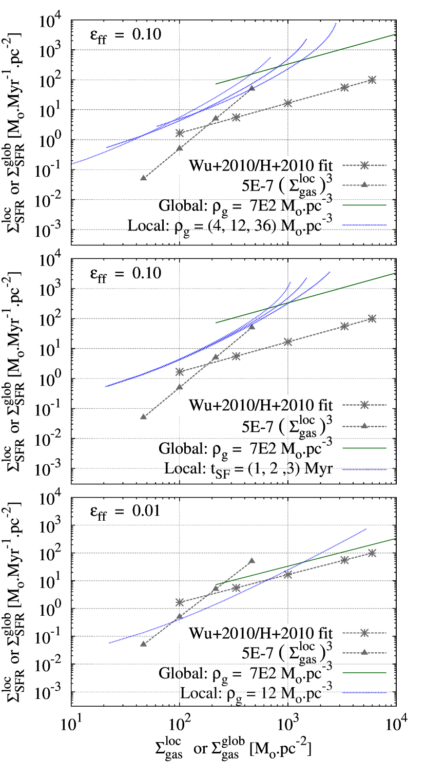
Figure 6.— Comparison between the locii of the data (dashed grey lines with asterisks and triangles) and model predictions (solid green line and dotted blue lines). Top panel: variation of the mean volume density of the low-density clump, 4, 12, and 36 $M_{\odot}\cdot pc^{-3}$ (dotted blue lines from left to right). Middle panel: variation of the time-span elapsed since star formation onset, $t_{SF}=3,2,1$ Myr (blue dotted lines from left to right). Bottom panel: the star formation efficiency per free-fall time is decreased by an order of magnitude, i.e. $\epsilon_{\rm ff}=0.01$.

While the top and bottom panels of Fig. 5 are qualitatively similar, they nevertheless present quantitative differences. These include: a predicted slope shallower than that observed for the local star formation relation, and different normalizations for both the global and local relations.

In Fig. 6, we vary the model parameters to see whether the match between model and observations can be improved. Dashed (grey) lines with asterisks and triangles show the locii of the diagram occupied by the observations. The global and local models are depicted as the (solid) green and (dotted) blue lines, respectively. In the top panel, the mean volume density of the low-density clump is varied by almost an order of magnitude, from 4 to 36 $M_{\odot}\cdot pc^{-3}$. With a higher volume density, the local star formation relation reaches higher surface densities, but without changing its slope or normalization markedly. In the middle panel, the local relation is presented for various time-spans since star formation onset, i.e. $t_{SF}=1,2$ and 3 Myr. A difference is noticeable in the high-density regime, which corresponds to the clump central regions where the free-fall time is shorter hence gas depletion quicker: longer time-spans yield smaller gas surface densities, as expected, but do not affect the overall trend. In the bottom panel, we decrease the star formation efficiency per free-fall time by an order of magnitude, i.e. $\epsilon_{\rm ff}=0.01$ instead of $\epsilon_{\rm ff}=0.1$ in the top and middle panels. The models and the data now occupy similar locii in the ($\Sigma_{\rm gas}$, $\Sigma_{\rm SFR}$) diagram, although the discrepancy in the slope of the local relation remains. As we saw in Section 3, steepening the model slope could be obtained by increasing the star formation efficiency per free-fall time with the gas density. Another possibility is that the local relation inferred by Heiderman et al. (2010) is artificially steepened as a consequence of binning the data in visual extinction hence gas surface density (Lombardi, Lada & Alves, 2013). If this is the case, their observed local relation cannot be used to estimate the star formation efficiency per free-fall time.

Using the mean star formation relation of Gutermuth et al. (2011) (see Eq. 20 in this paper), Parmentier, Pfalzner & Grebel (2014) estimate the star formation efficiency per free-fall time to be between 3 and 10 %, depending on the adopted duration of the Class II phase (see also Parmentier & Pfalzner, 2013). In contrast, the bottom panel of Fig. 6 shows that $\epsilon_{\rm ff}=0.01$ is still slightly too large for the high-density model (solid green line) to match the location of the HCN 1-0 clumps of Wu et al. (2010) (dashed line with asterisks). We indeed saw in the top panel of Fig. 2 that the high-density clump data suggest $\epsilon_{\rm ff}=0.5$ %. How can that value be reconciled with the significantly higher estimate of Parmentier, Pfalzner & Grebel (2014)? There might be different explanations.

5.1. Underestimated clump infrared luminosity

The total infrared luminosity of the clumps in Wu et al. (2010) is underestimated as a result of being derived from the four $IRAS$ bands (see Eq. 3 in Wu et al., 2010). Vutisalchavakul & Evans (2013) note that most clumps are extended sources, i.e. the average source size is larger than the $IRAS$ beam. They therefore re-estimate the infrared fluxes by performing aperture photometry of the clumps, instead of adopting the data from the $IRAS$ point-source catalog. Vutisalchavakul & Evans (2013) note that their $L_{IR}$ estimate is higher than what is obtained from the $IRAS$ point-source catalog by a factor of two on average. We illustrate this in Fig. 7 which compares the infrared luminosities of dense molecular clumps as obtained by Wu et al. (2010) and Vutisalchavakul & Evans (2013). Doubling the clump infrared luminosity raises the global star formation relation by a factor of two in the ($\Sigma_{\rm gas}$, $\Sigma_{\rm SFR}$) parameter space and yields therefore twice as high an estimate of the $\epsilon_{\rm ff}$, i.e. $\epsilon_{\rm ff}=0.01$ rather than $\epsilon_{\rm ff}=0.005$.

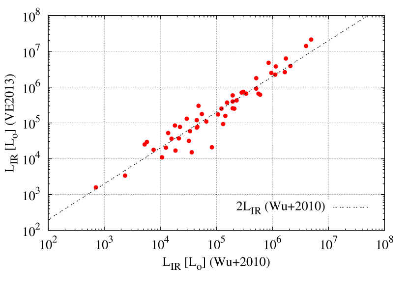
Figure 7.— Comparison between the infrared luminosities of dense molecular clumps as obtained by Wu et al. (2010) and Vutisalchavakul & Evans (2013) ($x$- and $y$-axis, respectively). The luminosities derived by Vutisalchavakul & Evans (2013) are a factor of about two higher than those derived by Wu et al. (2010) because their adopted aperture is larger than the $IRAS$ beam size

5.2. Overestimated $L_{IR}$ - $SFR$ ratio

Although most of the stellar light is reprocessed into the infrared for both starburst galaxies and dense molecular clumps, Krumholz & Tan (2007) point out that Eq. 5 is not appropriate to recover the star formation rate of individual clumps from their infrared luminosity. This issue is also discussed by Heiderman et al. (2010) who quote that the $L_{IR}-SFR$ calibration of Kennicutt (1998b) is likely to underestimate the star formation rate of an individual molecular clump. This is because during the first few Myr of star formation inside a clump, the ratio between its infrared luminosity and star formation rate is lower than given by Eq. 5, even when the stellar initial mass function is evenly populated up to its upper mass limit. Figure 1 in Krumholz & Tan (2007) shows that the ratio between the luminosity and star formation rate of a stellar population is lower than the Kennicutt (1998b) relation by a factor of 5 at $t_{SF}\simeq 1$ Myr and by a factor of 10 at $t_{SF}\simeq 0.5$ Myr (see also Urban, Martel & Evans (2010) and section 3.2 of Heiderman et al. (2010) for a discussion). The situation is even worse for forming-clusters not massive enough to sample the full mass range of the stellar IMF. In the case of the Orion A and Orion B clouds, Lada et al. (2012) show that the star formation rate obtained from the FIR-luminosity underestimates that obtained from direct-YSO counting by a factor of 8.

These two factors – time-evolving infrared luminosity and under-sampling of the stellar IMF – therefore yield luminosity-to-star formation rate ratios significantly lower than what is given by Eq. 5. Thus the observed star formation relation of dense clumps (grey line with asterisks in Fig. 6), obtained from Eq. 5, may underestimate the actual star formation rate surface density. Accordingly, the clump $\epsilon_{\rm ff}$ may be higher than the 1 %-estimate inferred in Section 5.1. That is, if Eq. 5 is higher than the actual luminosity-to-star formation rate ratio by a factor of 5, the clump star formation rate derived from Eq. 5 will be underestimated by a factor of 5, and so will be the estimated star formation efficiency per free-fall time. Therefore, the dense-clump data of Wu et al. (2010) do not exclude $\epsilon_{\rm ff}$ estimates of a few percent. We also note that the majority of the clumps studied by Wu et al. (2010) have masses smaller than 3000 $M_{\odot}$ (their fig. 30). They will therefore produce stellar populations where the high-mass tail of the stellar IMF is not, or poorly, sampled (although a fraction of star formation may occur at densities lower than $\simeq 700\,M_{\odot}\cdot pc^{-3}$, i.e. beyond the HCN $1-0$ half-peak contour; see figs. 1 and 7 in Parmentier & Pfalzner, 2013). The small cluster mass would strengthen the discrepancy between Eq. 5 and the actual luminosity-to-star formation rate ratio of the clumps, leading to even greater upward corrections of their star formation efficiency per free-fall time.

And there is yet another source of uncertainty in deriving the star formation rate of a clump from its infrared luminosity. This additional uncertainty is related to the clump star formation history. Figure 1 in Krumholz & Tan (2007) builds on a constant rate of star formation. Yet, indications of a star formation activity declining with time have been obtained for some star-forming regions, e.g. Chamaeleon I (Luhman, 2007; Belloche et al., 2011). For molecular clumps in near-equilibrium, a decrease with time of their star formation rate is expected as a result of gas depletion as stars form, and of the corresponding increase of the clump free-fall time (see Parmentier, Pfalzner & Grebel, 2014, for an in-depth discussion). An additional requirement to convert the clump infrared luminosity into their star formation rate is therefore a model accounting for the actual star formation history, which may not be one of a constant star formation rate.

Finally, we note that, even on a galaxy scale, Chomiuk & Povik (2011) recommend an upward revision of extragalactic star formation rates.

5.3. Overestimated local star formation relation?

It may also be that Parmentier & Pfalzner (2013) overestimated the star formation efficiency per free-fall time because the star formation relation of Gutermuth et al. (2011) is itself overestimated.

Lombardi, Lada & Alves (2013) find that, for the Orion-A molecular cloud, the surface density of protostars (in number counts) is:

$$\Sigma_{proto}\simeq 1.65\left(\frac{A_{K}}{mag}\right)^{2.03}[{\rm stars}\cdot pc^{-2}]\,,$$ (21)

with $A_{K}$ the extinction in the $K$-band. Adopting a mean YSO mass of $0.5M_{\odot}$ and the conversion $\frac{\Sigma_{\rm gas}}{M_{\odot}\cdot pc^{-2}}=197\frac{A_{k}}{mag}$ gives (in mass counts):

$$\Sigma_{\star}=2\cdot 10^{-5}\Sigma_{\rm gas}^{2.03}\,,$$ (22)

with $\Sigma_{\star}$ and $\Sigma_{\rm gas}$ in units of $M_{\odot}\cdot pc^{-2}$.

This is a factor of 50 less than found by Gutermuth et al. (2011). It is important to realize, however, that the star formation relation of Gutermuth et al. (2011) covers Class I and Class II objects, while Lombardi, Lada & Alves (2013) include only Class I protostars. Given that in nearby star-forming regions the total number of Class I and Class II objects is higher than the number of Class I objects by a factor of 3-to-10 (see Table 1 in Gutermuth et al., 2011), the actual discrepancy between Eq. 20 and Eq. 22 is probably no higher than a factor of 10. One might speculate that the lower normalization found by Lombardi, Lada & Alves (2013) is conducive to a $\epsilon_{\rm ff}$-estimate lower than the 10 % found by Parmentier & Pfalzner (2013) (see also Lada et al., 2013, for a detailed discussion of the Orion A and B data, and of the role played by the resolution of the extinction maps).

In summary, there are various possibilities to bridge the gap between the $\epsilon_{\rm ff}$ as estimated for individual molecular clumps ($\epsilon_{\rm ff}\simeq 0.5$ %, top panel of Fig. 2) and for star-forming clouds of the Solar Neighbourhood ($\epsilon_{\rm ff}\simeq 3-10$ %, Parmentier, Pfalzner & Grebel, 2014). (i) The $\epsilon_{\rm ff}$ derived for molecular clumps is underestimated because of an underestimated clump infrared luminosity (Section 5.1). (ii) The star formation rate of clumps may be underestimated when using the Kennicutt (1998b) relation (Eq. 5) as this one was established for galaxies, and is not suitable for molecular clumps whose hosted cluster is not fully developed yet (Section 5.2). (iii) On the other hand, the $\epsilon_{\rm ff}$ obtained by Parmentier & Pfalzner (2013) may be too high because the local star formation relation of Gutermuth et al. (2011) overestimates the surface density of YSOs at a given gas surface density (Section 5.3). A detailed comparison of the various star formation relations for nearby molecular clouds is beyond the scope of our paper, however.

6. Conclusions

The key-points to be taken from our paper are the following:

- The change of slope between the local and global star formation relations results from two different ways of measuring the gas and star formation rate surface densities of molecular clumps. The global relation describes how the clump mean surface densities relate to each other. To define it observationally therefore requires a population of clumps. In contrast, the local relation relates the gas and star formation rate surface densities measured in a set of nested intervals inside a given clump. As such, a local relation can be obtained for one single clump already (see Fig. 1). Whether the gas and star surface densities are measured globally or locally leads to different star formation relations even when the underlying physics of star formation is the same. We refer the combined local and global star formation relations as a composite star formation relation.

- As a result of the above definitions, the local star formation relation has so far been measured in nearby molecular clouds only, since their YSOs can be detected on a one-by-one basis. A global star formation relation can be obtained for both nearby molecular clouds, and distant compact molecular clumps (see Heiderman et al., 2010; Lada et al., 2013). In this paper, we have considered the global relation of distant high-density clumps.

- That the slope of the local relation for nearby molecular clouds is steeper than that of the global relation for distant compact clumps does not necessarily imply that star formation becomes less efficient with decreasing gas surface densities. Actually, the slope of the star formation relation also depends on how measurements are performed, i.e., on a global or local scale. A similar conclusion is reached by Lada et al. (2013) about giant molecular clouds: there is a local star formation relation within them, but no global star formation relation between them.

- Contrary to distant molecular clumps, nearby molecular clouds are devoid of massive stars. Again, that difference is not necessarily the reason as to why the global and local star formation relations differ.

- That nearby-cloud regions and distant compact clumps show different star formation rate surface densities at a given gas surface density can be explained by the different nature of the local and global relations. It does not necessarily require the $SFR-L_{IR}$ relation to be re-calibrated.

- It is crucial not to apply a global star formation relation to locally-made measurements as one would otherwise wrongly infer that the star formation efficiency per free-fall time increases with gas density.

- A power-law index $N$ for the global star formation relation different from $1.5$ does not necessarily preclude that a fixed fraction of gas is converted into stars every free-fall time. The slope of the global relation is driven by the mode of star formation (i.e. is the star formation efficiency per free-fall time constant, or is it gas-density dependent?), and by the clump mass-radius relation.

References

- Belloche et al. (2011) Belloche, A., Schuller, F., Parise, B., et al. 2011, A&A 527, 145
- Bigiel et al. (2008) Bigiel, F., Leroy, A., Walter, F., et al. 2008, AJ 136, 2846
- Bell et al. (2013) Bell, C.P.M., Naylor, T., Mayne, N.J., Jeffries, R.D., Littlefair, S.P. 2013, MNRAS 434, 806
- Chomiuk & Povik (2011) Chomiuk, L., Povich, M.S. 2011, AJ 142, 197
- Dib et al. (2011) Dib, S., Piau, L., Mohanty, S., Braine, J. 2013, MNRAS 436, 3727
- Evans et al. (2009) Evans, N.J., Dunham, M.M., Jorgensen, J.K., et al. 2009, ApJS, 181, 321
- Evans, Heiderman & Vutisalchavakul (2014) Evans, N.J., II; Heiderman, A. & Vutisalchavakul, N. 2014, ApJ 782, 114
- Fritze-von Alvensleben & Gerhard (1994) Fritze-v. Alvensleben, U., Gerhard, O. E., 1994, A&A, 285, 751-774
- Gao & Solomon (2004) Gao, Y.; Solomon, P.M., 2004, ApJ, 606, 271
- Gutermuth et al. (2011) Gutermuth, R.A., Pipher, J.L., Megeath, S.T., et al. 2011, ApJ, 739, 84
- Heiderman et al. (2010) Heiderman, A.; Evans, N.J., II; Allen, L.E.; Huard, T.; Heyer, M. 2010, ApJ 723, 1019
- Kennicutt (1998a) Kennicutt, R.C., Jr. 1998a, ApJ, 498, 541
- Kennicutt (1998b) Kennicutt, R.C., Jr. 1998b, ARA&A, 36, 189
- Kennicutt (2007) Kennicutt, R.C., Calzetti, D., Walter, F., et al. 2007, ApJ, 671, 333
- Krumholz & Tan (2007) Krumholz, M.R., Tan, J.C. 2007, ApJ, 654, 304
- Krumholz & Thompson (2007) Krumholz, M.R., Thompson, T.A. 2007, ApJ, 669, 289
- Krumholz, Deckel & McKee (2012) Krumholz, M.R., Deckel, A. & McKee, C.F. 2012, ApJ, 745, 69
- Lada, Lombardi & Alves (2010) Lada, C.J.; Lombardi, M.; Alves, J.F. 2010, ApJ 724, 867
- Lada et al. (2012) Lada, C.J.; Forbrich, J.; Lombardi, M.; Alves, J.F. 2012, ApJ 745, 190
- Lada et al. (2013) Lada, C.J.; Lombardi, M.; Roman-Zuniga, C.; Forbrich, J.; Alves, J.F. 2013, ApJ 778, 133