Symmetry-broken local-density approximation for one-dimensional systems

Abstract

Within density-functional theory, the local-density approximation (LDA) correlation functional is typically built by fitting the difference between the near-exact and Hartree-Fock (HF) energies of the uniform electron gas (UEG), together with analytic perturbative results from the high- and low-density regimes. Near-exact energies are obtained by performing accurate diffusion Monte Carlo calculations, while HF energies are usually assumed to be the Fermi fluid HF energy. However, it has been known since the seminal work of Overhauser that one can obtain lower, symmetry-broken (SB) HF energies at any density. Here, we have computed the SBHF energies of the one-dimensional UEG and constructed a SB version of the LDA (SBLDA) from the results. We compare the performance of the LDA and SBLDA functionals when applied to one-dimensional systems, including atoms and molecules. Generalization to higher dimensions is also discussed.

I Introduction

In 1965, Kohn and Sham Kohn and Sham (1965) showed that the knowledge of an analytical parametrization of the uniform electron gas (UEG) correlation energy Loos and Gill (2016) allows one to perform approximate calculations for atoms, molecules and solids. Parr and Yang (1989) This led to the development of various local-density approximation (LDA) correlation functionals (VWN, Vosko et al. (1980) PZ, Perdew et al. (1981) PW92, Perdew and Wang (1992) etc.), all of which require information on the high- and low-density regimes of the UEG, Loos and Gill (2013); Loos (2013); Loos et al. (2014); Loos (2014); Zia (1973); Isihara and Toyoda (1977); Rajagopal and Kimball (1977); Glasser (1977); Isihara and Ioriatti (1980); Glasser (1984); Seidl (2004); Chesi and Giuliani (2007); Loos and Gill (2011a); Macke (1950); Bohm and Pines (1953); Pines (1953); Gell-Mann and Brueckner (1957); DuBois (1959); Carr and Maradudin (1964); Misawa (1965); Onsager et al. (1966); Wang and Perdew (1991); Hoffman (1992); Endo et al. (1999); Ziesche and Cioslowski (2005); Sun et al. (2010); Loos and Gill (2011b, 2012a, c) and are parametrized using results from near-exact diffusion Monte Carlo (DMC) calculations. Lee and Drummond (2011); Tanatar and Ceperley (1989); Kwon et al. (1993); Rapisarda and Senatore (1996); Attaccalite et al. (2002, 2003); Gori-Giorgi et al. (2003); Drummond and Needs (2009); Ceperley and Alder (1980); Ballone et al. (1992); Ortiz and Ballone (1994, 1997); Kwon et al. (1998); Ortiz et al. (1999); Zong et al. (2002); Drummond et al. (2004); Spink et al. (2013)

The LDA is the simplest approximation within density-functional theory (DFT). Parr and Yang (1989) It assumes that a real, non-uniform system (such as a molecule or a solid) may be treated as a collection of infinitesimally-small UEGs of electronic density $\rho$. In principle, if one knows the reduced (i.e. per electron) correlation energy $e_{\text{c}}^{\text{FF}}(\rho)$ of the UEG for any density $\rho$, by summing the individual contributions over all space, it is therefore possible to obtain the LDA correlation energy

$$E_{\text{c}}^{\text{LDA}}=\int\rho(\bm{r})\,e_{\text{c}}^{\text{FF}}[\rho(\bm{r})]\,d\bm{r}.$$ (1)

Although it describes molecular bonding reasonably well compared to the Thomas-Fermi (TF) model Thomas (1927); Fermi (1927) (which approximates the kinetic energy using the TF functional and ignores the exchange interaction between same-spin electrons), this rather crude approximation has managed only mixed success. Tong and Sham (1966) In particular, the functional consistently overestimates correlation energies, giving rise to errors up to some factor of two. Parr and Yang (1989) Fortunately, errors in the exchange and correlation energies approximately compensate each other, thus generating a total energy that is usually in good agreement with experimental results. Ernzerhof et al. (1997)

Since the emergent days of DFT, the UEG correlation energy $e_{\text{c}}^{\text{FF}}(\rho)$ has always been defined as the difference between the exact energy $e(\rho)$ and the Fermi fluid Hartree-Fock (FFHF) energy $e_{\text{HF}}^{\text{FF}}(\rho)$. However, in the early sixties, Overhauser Overhauser (1959, 1962) showed that the FF state is never the Hartree-Fock (HF) ground state due to spin- and charge-density instabilities. Giuliani and Vignale (2005) Therefore, for any density, one can find a symmetry-broken HF (SBHF) solution which has a lower energy than the FFHF solution. Unfortunately, the exact character of this SBHF solution is not given, nor is it necessary for it to remain the same over the full density range.

Zhang and Ceperley Zhang and Ceperley (2008) have recently presented a computational “proof” of this statement. Performing unrestricted HF (UHF) calculations on the paramagnetic state of finite-size three-dimensional UEGs, they have succeeded in finding a ground state with broken spin-symmetry in the high-density region. For lower densities, Trail et al. discovered that the Wigner crystal (WC) is more stable than the FF state for $r_{s}>1.44$ in 2D and $r_{s}>4.5$ in 3D, Trail et al. (2003) where the Wigner-Seitz radius $r_{s}$ is the average distance between electrons. These calculations were recently refined by Holzmann and coworkers. Delyon et al. (2008); Bernu et al. (2008, 2011); Baguet et al. (2013, 2014); Delyon et al. (2015)

Physically, a WC represents a state whose energy is dominated by the potential energy term, resulting in the electrons localizing on lattice points. This situation typically occurs at low densities, where the WC becomes the ground state. At high densities the kinetic energy dominates and the delocalized FF is the ground state. In addition to the usual FF and WC phases, they have also considered incommensurate crystals (a state in which the number of the charge density maxima is higher than the number of electrons), showing that such a phase is always favored over the FF; independently of the imposed polarization and crystal symmetry and in agreement with the earlier prediction of Overhauser. Overhauser (1959, 1962)

Here, we propose to construct a symmetry-broken version of the LDA, taking the one-dimensional (1D) UEG as an example, and using SBHF energies instead of the usual FFHF expression. From an experimental point of view, 1D systems have recently attracted much attention due to their practical realization in carbon nanotubes, Saito et al. (1998); Egger and Gogolin (1998); Bockrath et al. (1999); Ishii et al. (2003); Shiraishi and Ata (2003) organic conductors, Schwartz et al. (1998); Vescoli et al. (2000); Lorenz et al. (2002); Dressel et al. (2005); Ito et al. (2005) transition metal oxides, Hu et al. (2002) edge states in quantum Hall liquids, Milliken et al. (1996); Mandal and Jain (2001); Chang (2003) semiconductor heterostructures, Gonï et al. (1991); Auslaender et al. (2000); Zaitsev-Zotov et al. (2000); Liu et al. (2005); Steinberg et al. (2006) confined atomic gases, Monien et al. (1998); Recati et al. (2003); Moritz et al. (2005) and atomic or semiconducting nanowires. Schäfer et al. (2008); Huang et al. (2001)

This article is organized as follows. In Sec. II, we introduce the paradigm we have used to create a strict 1D UEG. Section III covers the acquisition of accurate SBHF energies at various densities, followed by the definition of the two correlation functionals in Sec. IV. These are compared in Sec. V for 1D systems, including atoms and molecules. Unless otherwise stated, atomic units are used throughout.

Table 1: $\Delta e_{\text{HF}}^{\text{SB}}$ (in millihartree) for various $n$ and $r_{s}$. $r_{s}^{\text{SB}}$ is the lowest value of $r_{s}$ for which one can find a SBHF solution.

		Wigner-Seitz radius $r_{s}=1/(2\rho)$
$n$	$r_{s}^{\text{SB}}$	0.5	1	2	5	10	15	20	50	75	100
9	1.22	$0$	$0$	$2.685$	$6.852$	$6.226$	$5.187$	$4.392$	$2.267$	$1.628$	$1.273$
19	0.79	$0$	$0.666$	$5.042$	$7.695$	$6.621$	$5.445$	$4.583$	$2.346$	$1.678$	$1.311$
29	0.64	$0$	$1.576$	$5.525$	$7.860$	$6.698$	$5.496$	$4.621$	$2.361$	$1.688$	$1.319$
39	0.55	$0$	$1.985$	$5.700$	$7.920$	$6.727$	$5.515$	$4.635$	$2.366$	$1.692$	$1.321$
49	0.50	$0$	$2.188$	$5.784$	$7.949$	$6.741$	$5.524$	$4.642$	$2.369$	$1.694$	$1.323$
59	0.46	$0.000$	$2.302$	$5.830$	$7.965$	$6.749$	$5.529$	$4.646$	$2.370$	$1.695$	$1.324$
69	0.43	$0.008$	$2.371$	$5.859$	$7.975$	$6.754$	$5.532$	$4.648$	$2.371$	$1.695$	$1.324$
79	0.41	$0.143$	$2.418$	$5.878$	$7.982$	$6.757$	$5.534$	$4.650$	$2.372$	$1.695$	—
89	0.40	$0.198$	$2.450$	$5.891$	$7.986$	$6.759$	$5.535$	$4.651$	$2.372$	—	—
99	0.38	$0.244$	$2.473$	$5.901$	$7.989$	$6.760$	$5.536$	$4.652$	—	—	—
109	0.36	$0.281$	$2.490$	—	—	—	—	—	—	—	—
119	0.35	$0.312$	$2.503$	—	—	—	—	—	—	—	—
129	0.35	$0.337$	—	—	—	—	—	—	—	—	—
$\vdots$	$\vdots$	$\vdots$	$\vdots$	$\vdots$	$\vdots$	$\vdots$	$\vdots$	$\vdots$	$\vdots$	$\vdots$	$\vdots$
$\infty$	0	$0.476$	$2.570$	$5.938$	$8.002$	$6.767$	$5.540$	$4.655$	$2.372$	$1.695$	$1.324$

II One-dimensional uniform electron gas

A 1D UEG is constructed by confining a number $n$ of interacting electrons to a ring of radius $R$ of electronic density Loos and Gill (2012b, 2013); Loos et al. (2014); Tognetti and Loos (2016)

$$\rho=\frac{n}{2\pi R}=\frac{1}{2r_{s}}.$$ (2)

where $r_{s}$ is the so-called Wigner-Seitz radius. Giuliani and Vignale (2005); Parr and Yang (1989) We refer the readers to Ref. Loos and Gill, 2013 for more details about this paradigm, which has been shown to be equivalent to the more conventional “electrons-in-a-periodic-box” model in the thermodynamic limit (i.e. $n\to\infty$), Loos and Gill (2011c, 2013); Loos (2013, 2014) but mathematically simpler. Loos and Gill (2011c) This can be qualitatively explained by the “short-sightedness” of the electronic matter. Kohn (1996); Prodan and Kohn (2005) Because the paramagnetic and ferromagnetic states are degenerate in strict 1D systems, we will consider only the spin-polarized electron gas. Astrakharchik and Girardeau (2011); Lee and Drummond (2011); Loos and Gill (2012b, 2013); Loos (2013); Loos et al. (2014); Loos (2014); Loos et al. (2015)

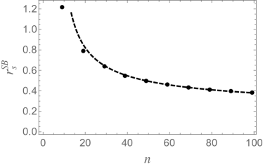
Figure 1: $r_{s}^{\text{SB}}$ as a function of $n$. The dashed curve represents the fit defined by Eq. (11)

The expression of the (non-symmetry-broken) FFHF energy is Loos and Gill (2013)

$$e_{\text{HF}}^{\text{FF}}(r_{s},n)=\frac{t_{\text{HF}}(n)}{r_{s}^{2}}+\frac{v_{\text{HF}}(n)}{r_{s}},$$ (3)

with

$$t_{\text{HF}}(n) =\frac{\pi^{2}}{24}\frac{n^{2}-1}{n^{2}},$$ (4a)

$$v_{\text{HF}}(n) =\left(\frac{1}{2}-\frac{1}{8n^{2}}\right)\left[\psi\left(n+\frac{1}{2}\right)-\psi\left(\frac{1}{2}\right)\right]-\frac{1}{4},$$ (4b)

where $\psi(x)$ is the digamma function. Olver et al. (2010) This corresponds to occupying the $n$ lowest plane waves

$$\phi_{m}(\theta)=\frac{\exp\left(im\theta\right)}{\sqrt{2\pi R}},$$ (5)

where $\theta$ is the angle of the electron around the ring and $m\in\mathbb{Z}$. The FFHF energy (3) diverges logarithmically for large numbers of electrons, Schulz (1993); Fogler (2005); Fogler and Pivovarov (2005); Loos and Gill (2013)

$$e_{\text{HF}}^{\text{FF}}(r_{s},n)\sim\frac{\ln\sqrt{n}}{r_{s}}+O(1),$$ (6)

but an identical divergence in the exact energy $e(r_{s},n)$ results in a finite correlation energy

$$e_{\text{c}}^{\text{FF}}(r_{s},n)=e(r_{s},n)-e_{\text{HF}}^{\text{FF}}(r_{s},n).$$ (7)

As stated in Sec. I, our goal here is to determine the SB correlation energy in the thermodynamic limit

$$e_{\text{c}}^{\text{SB}}(r_{s})=\lim_{n\to\infty}e_{\text{c}}^{\text{SB}}(r_{s},n)$$ (8)

via extrapolation, where

$$\begin{split}e_{\text{c}}^{\text{SB}}(r_{s},n)&=e(r_{s},n)-e_{\text{HF}}^{\text{SB}}(r_{s},n)\\ &=e(r_{s},n)-e_{\text{HF}}^{\text{FF}}(r_{s},n)+\Delta e_{\text{HF}}^{\text{SB}}(r_{s},n)\\ &=e_{\text{c}}^{\text{FF}}(r_{s},n)+\Delta e_{\text{HF}}^{\text{SB}}(r_{s},n).\end{split}$$ (9)

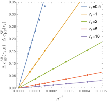
Figure 2: $\Delta e_{\text{HF}}^{\text{SB}}(r_{s},n)$ as a function of $n^{-2}$ for various $r_{s}$.

III Symmetry-broken Hartree-Fock calculations

In order to obtain SBHF energies, we have written a self-consistent field program Szabo and Ostlund (1989) using plane waves of the form (5) with

$$m=-\frac{M-1}{2},\ldots,\frac{M-1}{2},$$ (10)

where we have used up to $M=399$ to ensure that our energies are always converged within microhartree accuracy. As expected, large $r_{s}$ values require larger basis sets in order to converge the energy to the same accuracy due to the local character of the WC. Loos and Gill (2009a) The required one- and two-electron integrals can be found in Ref. Loos and Gill, 2013. The results are reported in Table 1, where we have also reported $r_{s}^{\text{SB}}$, the lowest $r_{s}$ value for which one can find a SBHF solution. It is interesting to note that $r_{s}^{\text{SB}}$ converges extremely slowly with respect to $n$, as shown in Fig. 1. We have found that the following function (see Appendix A)

$$r_{s}^{\text{SB}}(n)=\frac{a}{\ln n+b}$$ (11)

(with $a=1.13535$ and $b=-1.61346$) fits our data well. Equation (11) reveals that, in order to observe a SBHF solution below $r_{s}=0.2$, one needs at least 1500 electrons.

We have obtained the thermodynamic values by extrapolation via the following asymptotic form:

$$\Delta e_{\text{HF}}^{\text{SB}}(r_{s},n)=\Delta e_{\text{HF}}^{\text{SB}}(r_{s})+A\,n^{-2}.$$ (12)

For each $r_{s}$ value we have used the six largest $n$ values of Table 1, except for $r_{s}=0.5$ where only the last three terms were considered. The quality of the fit is demonstrated in Fig. 2. A similar expression to (12) has been used by Lee and Drummond to extrapolate DMC calculations to the thermodynamic limit. Lee and Drummond (2011)

Physically, the appearance of the SBHF solution is characterized by the formation of a WC, i.e. where the electrons have “crystallized” such that they are separated by an angle of $2\pi/n$. Schulz (1993); Fogler (2005); Fogler and Pivovarov (2005); Loos and Gill (2013) This phenomenon is easily understood in terms of the behaviour of the kinetic and potential energies with respect to $r_{s}$, which scale as $r_{s}^{-2}$ and $r_{s}^{-1}$ respectively (see Eq. (3)). Therefore, at small $r_{s}$, occupying the $n$ lowest plane waves is energetically favorable, as it minimizes the dominant kinetic energy contribution. However, there exists a critical density $r_{s}^{\text{SB}}$ for which it becomes compelling to break the spatial symmetry, (by populating higher plane waves) albeit at the expense of a meagre increase in the kinetic energy. This has the effect of lowering the potential energy by localizing the electrons, and in doing so, effectively reducing the interelectronic interaction.

The formation of a Wigner crystal is illustrated in Fig. 3 where we have represented the HF and SBHF densities for 19 electrons at $r_{s}=5$. One can see that, when the WC forms, a gap opens at the Fermi surface between the occupied and vacant orbitals. As shown in Table 2, the symmetry-breaking stabilization has a very significant effect on the values of the correlation energy, especially at intermediate and low densities where it represents a large fraction of the total correlation energy. These results confirm Overhauser’s prediction that in the thermodynamic limit, it is always favorable to break the spatial symmetry (see Appendix A). We have, however, observed that the stabilization becomes extremely small at high density.

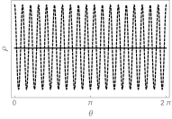
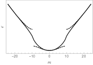
Figure 3: Electronic density $\rho$ as a function of $\theta$ (left) and orbital energies $\epsilon$ as a function of $m$ (right) for the HF (solid line) and SBHF (dashed line) solutions for $n=19$ at $r_{s}=5$.

Table 2: Correlation energies (in millihartree) in the thermodynamic limit for various $r_{s}$.

$r_{s}$	$-e_{\text{c}}^{\text{FF}}$	$-e_{\text{c}}^{\text{SB}}$	$1-e_{\text{c}}^{\text{SB}}/e_{\text{c}}^{\text{FF}}$
0	$27.416$	$27.416$	0%
0.5	$23.962$	$23.486$	2%
1	$21.444$	$18.874$	12%
2	$17.922$	$11.984$	33%
5	$12.318$	$4.316$	65%
10	$8.292$	$1.525$	82%
15	$6.319$	$0.779$	88%
20	$5.133$	$0.478$	91%
50	$2.476$	$0.104$	96%
100	$1.358$	$0.034$	97%

IV Correlation functionals

IV.1 Local-density approximation

In this study, we used the LDA functional developed in Ref. Loos, 2013, which has been constructed using the “robust” interpolation proposed by Cioslowski Cioslowski et al. (2012)

$$e_{\text{c}}^{\text{LDA}}(r_{s}) =t^{2}\sum_{j=0}^{3}c_{j}t^{j}(1-t)^{3-j},$$ (13)

$$t =\frac{\sqrt{1+4\,k\,r_{s}}-1}{2\,k\,r_{s}},$$ (14)

with

$$c_{0} =k\,\eta_{0}, c_{1} =4\,k\,\eta_{0}+k^{3/2}\eta_{1},$$

$$c_{2} =5\,\varepsilon_{0}+\varepsilon_{1}/k, c_{3} =\varepsilon_{0},$$

and the high- and low-density expansions, Loos (2013)

$$e_{\text{c}}(r_{s})=\varepsilon_{0}+\varepsilon_{1}\,r_{s}+O(r_{s}^{2}),\qquad r_{s}\ll 1,$$ (15a)

$$e_{\text{c}}(r_{s})=\frac{\eta_{0}}{r_{s}}+\frac{\eta_{1}}{r_{s}^{3/2}},+O(r_{s}^{-2}),\qquad r_{s}\gg 1,$$ (15b)

where

$$\varepsilon_{0} =-\frac{\pi^{2}}{360}, \varepsilon_{1} =+0.00845,$$

$$\eta_{0} =-\ln(\sqrt{2\pi})+3/4, \eta_{1} =+0.359933,$$

and $k=0.418268$ is a scaling factor, determined by a least-squares fit of the DMC data given in Refs. Lee and Drummond, 2011 and Loos and Gill, 2013. As reported in Ref. Loos, 2013, the LDA and DMC correlation energies agree to within 0.1 millihartree.

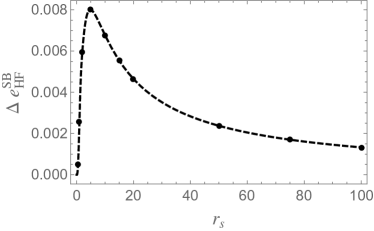
Figure 4: $\Delta e_{\text{HF}}^{\text{SB}}$ as a function of $r_{s}$ in the thermodynamic limit. The dashed curve represents the fit defined by Eq. (17)

IV.2 Symmetry-broken local-density approximation

We define the SBLDA functional as

$$e_{\text{c}}^{\text{SBLDA}}(r_{s})=e_{\text{c}}^{\text{LDA}}(r_{s})+\Delta e_{\text{HF}}^{\text{SB}}(r_{s}),$$ (16)

where $e_{\text{c}}^{\text{LDA}}(r_{s})$ is given by (13). We propose to use the following expression for the symmetry-breaking stabilization:

$$\Delta e_{\text{HF}}^{\text{SB}}(r_{s})=r_{s}^{2}\frac{a_{0}+a_{1}r_{s}+a_{2}r_{s}^{2}-\eta_{0}r_{s}^{3}}{b_{0}+b_{1}r_{s}^{5}+b_{2}r_{s}^{11/2}+r_{s}^{6}}$$ (17)

where

$$a_{0} =-0.0646228, a_{1} =0.535062, a_{2} =-0.490719,$$

$$b_{0} =53.1171, b_{1} =1.53114, b_{2} =2.19606.$$

The expression (17) is illustrated in Fig. 4 alongside the corresponding data of Table 2. The quality of (17) is excellent with a maximum error of 7 microhartrees compared to the values reported in Table 1.

In the low-density limit, Eq. (17) behaves as

$$\Delta e_{\text{HF}}^{\text{SB}}(r_{s})=-\frac{\eta_{0}}{r_{s}}+O(r_{s}^{-3/2}),{\color[rgb]{0,0,0}\qquad r_{s}\gg 1,}$$ (18)

which, when combined with Eqs. (15b) and (16), gives

$$e_{\text{c}}^{\text{SBLDA}}(r_{s})=O(r_{s}^{-3/2}),\qquad r_{s}\gg 1.$$ (19)

This behaviour is a direct consequence of the SBHF treatment allowing the electrons to localize at low densities, unlike the FFHF solution. It is therefore able to correctly identify the appearance of the WC phase, which results in the low-density expansion of the SBHF solution matching that of the exact energy up to $O(r_{s}^{-3/2})$. This difference in low-density behaviour creates an important distinction between $e_{\text{c}}^{\text{LDA}}$ and $e_{\text{c}}^{\text{SBLDA}}$. For small $r_{s}$, we have imposed $\Delta e_{\text{HF}}^{\text{SB}}(r_{s})$ to be quadratic in $r_{s}$, as shown in Appendix A.

Table 3: Ionization energy and electron affinity (in eV) of 1D atoms calculated with various methods.

	Ionization energy			Electron affinity
Atom	A -¿ A+ + e-			A + e- -¿ A-
	MP3	LDA	SBLDA	MP3	LDA	SBLDA
H	13.606	14.125	14.013	3.893	4.327	4.154
He	33.895	34.393	34.325	—	—	0
Li	4.522	4.895	4.712	1.395	1.717	1.512
Be	10.408	10.822	10.669	—	—	0
B	2.099	2.386	2.190	0.638	0.875	0.688
C	4.730	5.056	4.865	—	—	0
N	1.14	1.38	1.20	0.34	0.51	0.37
O	2.56	2.83	2.63	—	—	—
F	0.68	0.87	0.72	0.2	0.3	0.2
Ne	1.5	1.7	1.5	—	—	—

V Correlation energy in one-dimensional systems

In this Section, we test the LDA and SBLDA functionals defined in Secs. IV.1 and IV.2, respectively. The LDA and SBLDA correlation energies are obtained via

$$E_{\text{c}}^{\text{LDA/SBLDA}}=\int\rho(x)e_{\text{c}}^{\text{LDA/SBLDA}}[\rho(x)]dx.$$ (20)

which is computed by numerical quadrature. These quantities are calculated with the HF density, i.e. they are not calculated self-consistently. Pople et al. (1992) However, as expected, Johnson et al. (1993) we have observed that the differences between self- and non-self-consistent densities are extremely small. Loos et al. (2014); Loos (2014) In some cases, we have also reported the exact, MP2 and MP3 energies. Szabo and Ostlund (1989); Helgaker et al. (2000) For additional information about these calculations, we refer the readers to Refs. Loos et al., 2014 and Loos et al., 2015 where theoretical and computational details are provided.

Table 4: Equilibrium bond length $R_{\text{eq}}$, transition structure bond length $R_{\text{ts}}$, dissociation energy $E_{\text{disso}}$ and transition barrier $\Delta E_{\text{ts}}$ of 1D molecules calculated with various methods.

Method		Molecules
		H2+	HeH^2+	He2^3+	H2
Exact	$R_{\text{eq}}$	2.581	2.182	1.793	2.639
	$R_{\text{ts}}$	—	3.296	4.630	—
	$E_{\text{disso}}$	$-0.3307$	$+0.1697$	$+0.0131$	$-0.1859$
	$\Delta E_{\text{ts}}$	—	$+0.0209$	$+0.2924$	—-
HF	$R_{\text{eq}}$	2.581	2.182	1.793	2.636
	$R_{\text{ts}}$	—	3.296	4.630	—
	$E_{\text{disso}}$	$-0.3307$	$+0.1697$	$+0.0131$	$-0.1846$
	$\Delta E_{\text{ts}}$	—	$+0.0209$	$+0.2924$	—-
MP2	$R_{\text{eq}}$	2.581	2.182	1.793	2.637
	$R_{\text{ts}}$	—	3.296	4.630	—
	$E_{\text{disso}}$	$-0.3307$	$+0.1697$	$+0.0131$	$-0.1854$
	$\Delta E_{\text{ts}}$	—	$+0.0209$	$+0.2924$	—-
MP3	$R_{\text{eq}}$	2.581	2.182	1.793	2.638
	$R_{\text{ts}}$	—	3.296	4.630	—
	$E_{\text{disso}}$	$-0.3307$	$+0.1697$	$+0.0131$	$-0.1857$
	$\Delta E_{\text{ts}}$	—	$+0.0209$	$+0.2924$	—-
LDA	$R_{\text{eq}}$	2.573	2.176	1.790	2.627
	$R_{\text{ts}}$	—	3.291	4.630	—
	$E_{\text{disso}}$	$-0.3328$	$+0.1696$	$+0.0126$	$-0.1857$
	$\Delta E_{\text{ts}}$	—	$+0.0214$	$+0.2964$	—-
SBLDA	$R_{\text{eq}}$	2.564	2.172	1.788	2.619
	$R_{\text{ts}}$	—	3.285	4.619	—
	$E_{\text{disso}}$	$-0.3341$	$+0.1697$	$+0.0124$	$-0.1864$
	$\Delta E_{\text{ts}}$	—	$+0.0216$	$+0.2995$	—-

V.1 Two electrons in a box

As a simple example to illustrate the performance of the SBLDA functional, we have thoroughly studied the well-known system composed by two electrons in a box of length $L$. In particular, we report variations in the correlation energy as a function of $L$ obtained using the MP2, MP3, LDA and SBLDA methods. In the interest of completion, we have also calculated the exact correlation energy of this system using a Hylleraas-type (Hy) expansion. Hylleraas (1928, 1929, 1930, 1964); Loos and Gill (2010a) The results of this investigation are illustrated in Fig. 5, where the error in the correlation energy $\Delta E_{\text{c}}=E_{\text{c}}-E_{\text{c}}^{\text{Hy}}$ is resolved as a function of $L$. As expected, MP2 and MP3 yields reliable estimates of the correlation energy for this system. On the other hand, LDA returns a poor estimate of this energy. This discrepancy is especially clear in the high-density region (i.e. small $L$). By construction, LDA and SBLDA have similar performances at high densities. However, SBLDA is much more accurate than LDA at low densities, where stabilization returned from breaking the symmetry is most significant. Similar results are expected for different external potentials. Loos and Gill (2009b, 2010b, 2010c)

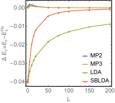
Figure 5: Error in correlation energy $\Delta E_{\text{c}}$ for two electrons in a box of length $L$ with MP2, LDA and SBLDA.

V.2 Atoms

We have calculated the ionization energies and electron affinities of 1D atoms Loos et al. (2015) using the Chem1D software developed by one of the authors. Ball and Gill (2015) The values obtained with the LDA and SBLDA functionals are compared to the MP3 values in Table 3, which has been observed to be an exceptionally accurate method in such systems.Loos et al. (2015) Overall, LDA and SBLDA overestimate the ionization energies and electron affinities for these systems. It is interesting to note that, although the performance of the LDA and SBLDA functionals are quite poor compared to MP3 for small atoms, the results become rapidly more accurate for larger atoms. In particular, we observe that the accuracy of SBLDA improves faster than LDA. For example, although the deviation between MP3 and SBLDA is only 0.04 eV for the ionization energy of the F atom, the LDA is still 0.19 eV off. This effect is most easily by acknowledging that larger atoms have more diffuse orbitals which possess lower density regions. Loos et al. (2015)

V.3 One-electron diatomics

As commonly reported, LDA-type functionals suffer from the self-interaction error (SIE), Merkle et al. (1992); Savin (1996); Perdew and Levy (1997); Zhang and Yang (1998); Tsuneda and Hirao (2014) i.e. the unphysical interaction of an electron with itself. This phenomenon is also known as the delocalization error and can be understood as the tendency of approximate functionals to artificially spread the electron density. Cohen et al. (2008a, b); Mori-Sánchez et al. (2008); Cohen et al. (2012) In Fig. 6, we have reported the SIE in the one-electron diatomic molecules H2+, HeH^2+ and He2^3+ as a function of the bond length. Although the SIE is obviously still present in SBLDA, one can see that it is less pronounced than it is in LDA. This statement is true at any bond length for the three molecules considered here. As an illustration, we have computed the energy of the H atom to be $-0.5$, $-0.519054$ and $-0.514971$ for HF, LDA and SBLDA, respectively.

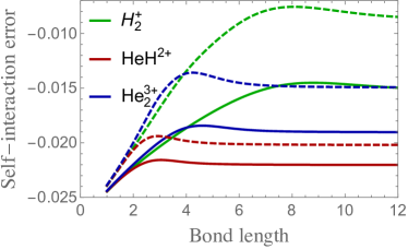
Figure 6: Self-interaction error in H2+ (green), HeH^2+ (red) and He2^3+ (blue) calculated with LDA (solid) and SBLDA (dashed) as a function of the bond length.

As reported in Table 4, the dissociation energy of H2+ is $-0.3307$, $-0.3328$ and $-0.3341$ for HF, LDA and SBLDA, respectively. Like in three dimensions, LDA and SBLDA slightly overestimate the binding energy of H2+. The equilibrium bond lengths are $2.581$, $2.573$ and $2.564$, showing that LDA and SBLDA predict bond lengths that are slightly too short.

As reported in Ref. Loos et al., 2015, HeH^2+ and He2^3+ are metastable, and it is instructive to know if LDA and SBLDA can predict this peculiar feature properly. Table 4 reports the equilibrium bond length of these molecules as well as the transition structure bond lengths and the height of the barrier. As we have observed in H2+, the bond lengths predicted by LDA and SBLDA are slightly too short while the transition state barriers are overestimated. It is interesting to note that both LDA and SBLDA predict (correctly) HeH^2+ and He2^3+ as being metastable species.

V.4 Dissociating H₂

The apparently simple problem of stretching H2 has been widely studied within DFT, as it reveals a common pitfall of approximate density functionals known as the static correlation error. Cohen et al. (2008a, c, 2012) Figure 7 displays the error in the correlation energy ($\Delta E_{\text{c}}$) of H2, as computed by the LDA and SBLDA functionals, as a function of the bond length. The exact results have been obtained with a James-Coolidge-type (JC) expansion. James and Coolidge (1933); Loos et al. (2015) Although the error in the SBLDA correlation energy is still significant, we observe a clear improvement for all bond lengths compared to LDA. This result is encouraging given the simplicity of the SBLDA functional.

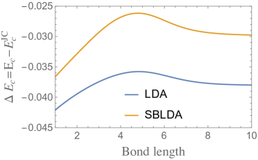
Figure 7: Error in correlation energy $\Delta E_{\text{c}}$ in H2 calculated with LDA and SBLDA as a function of the bond length.

Table 4 reports the equilibrium bond length of H2 as well as its dissociation energy obtained with HF, MP2, MP3, LDA and SBLDA. Compared to the exact results we observe, as previously reported, Loos et al. (2015) that MP2 and MP3 are extremely accurate in 1D. In contrast to the observations of Sec. V.3, the LDA slightly underestimates the dissociation energy here (agreeing with MP3), while the SBLDA continues to overestimate the same value. Both functionals, however, continue to yield a shorter bond length.

VI Discussion and concluding remarks

Inspired by Overhauser’s forecasts made some fifty years ago, we have constructed a symmetry-broken (SB) version of the commonly-used local-density approximation (LDA) for one-dimensional systems. The newly designed functional, which we have named SBLDA, has shown to surpass the performance of its LDA parent in providing better estimates of the correlation energy. More importantly, we believe that this functional could be potentially useful as a superior starting point for more accurate approximations within density-functional theory (DFT), such as generalized gradient approximations (GGAs) or hybrid functionals. Becke (2014) The methodology presented here is completely general and can be applied to higher-dimensional systems, where SB Hartree-Fock calculations have already been performed. Trail et al. (2003); Bernu et al. (2011); Baguet et al. (2013, 2014) The design of new exchange and correlation functionals for two- and three-dimensional systems based on the idea developed here is currently under progress in our group.

Appendix A Behavior of $\Delta e_{\text{HF}}^{\text{SB}}$ near $r_{s}^{\text{SB}}$

Near the critical density $r_{s}^{\text{SB}}$, it is possible to use a simple two-orbital model to study the symmetry-breaking process. When the symmetry breaking occurs, a small energy gap appears at the Fermi surface thanks to the mixing of the HOMO $\phi_{\pm\frac{n-1}{2}}(\theta)$ and LUMO $\phi_{\pm\frac{n+1}{2}}(\theta)$. Therefore, to study the behavior of $\Delta e_{\text{HF}}^{\text{SB}}$ near $r_{s}^{\text{SB}}$ (see Sec. IV.2), we consider the two orthonormalized molecular orbitals

$$\varphi_{1}(\theta) =\frac{\phi_{\frac{n-1}{2}}(\theta)+c\,\phi_{-\frac{n+1}{2}}(\theta)}{\sqrt{1+c^{2}}},$$ (21a)

$$\varphi_{2}(\theta) =\frac{\phi_{-\frac{n-1}{2}}(\theta)+c\,\phi_{\frac{n+1}{2}}(\theta)}{\sqrt{1+c^{2}}}.$$ (21b)

This two-orbital model teaches us that there exists a critical density

$$r_{s}^{\text{SB}}(n)=\frac{\pi^{2}/4}{\psi(n-1/2)+\frac{1}{2n-1}+\gamma+2(\ln 2-1)}$$ (22)

(where $\gamma$ is the Euler-Mascheroni constant Olver et al. (2010)) after which it is energetically favourable to mix these two orbitals, and the value

$$c^{2}=\frac{1-r_{s}^{\text{SB}}/r_{s}}{1+r_{s}^{\text{SB}}/r_{s}+\frac{4}{\pi^{2}}(\frac{1}{2n+1}+\frac{1}{2n-1})r_{s}^{\text{SB}}}$$ (23)

minimizes the energy for $r_{s}>r_{s}^{\text{SB}}$. Before $r_{s}^{\text{SB}}$, the solution is the usual FF state of energy

$$e_{\text{HF}}^{\text{FF}}(r_{s},n)=\frac{t_{\text{HF}}^{\text{FF}}(n)}{r_{s}^{2}}+\frac{v_{\text{HF}}^{\text{FF}}(n)}{r_{s}},$$ (24)

where

$$t_{\text{HF}}^{\text{FF}}(n) =\frac{\pi^{2}(n-1)^{2}}{4n^{2}},$$ (25a)

$$v_{\text{HF}}^{\text{FF}}(n) =\frac{\psi(n-1/2)+\gamma+2\ln 2}{n},$$ (25b)

minimizes the kinetic energy. However, for $r_{s}>r_{s}^{\text{SB}}$, this is outweighed by negative contributions in the potential term that drive the symmetry-breaking process. The kinetic and potential parts of the symmetry-breaking stabilization are given by

$$e_{\text{HF}}^{\text{SB}}(r_{s},n) =e_{\text{HF}}^{\text{FF}}(r_{s},n)-\Delta e_{\text{HF}}^{\text{SB}}(r_{s},n),$$ (26a)

$$\Delta e_{\text{HF}}^{\text{SB}}(r_{s},n) =\Delta t_{\text{HF}}^{\text{SB}}(r_{s},n)+\Delta v_{\text{HF}}^{\text{SB}}(r_{s},n),$$ (26b)

with

$$\Delta t_{\text{HF}}^{\text{SB}}(r_{s},n)=-\frac{\pi^{2}c^{2}}{(1+c^{2})nr_{s}^{2}},$$ (27)

$$\Delta v_{\text{HF}}^{\text{SB}}(r_{s},n)=\frac{4c^{2}}{(1+c^{2})^{2}nr_{s}}$$

$$\qquad\qquad\times\left[\frac{\pi^{2}/4}{r_{s}^{\text{SB}}(n)}-nc^{2}\left(\frac{1}{2n-1}-\frac{1}{2n+1}\right)\right].$$ (28)

In the thermodynamic limit, Eq. (22) yields

$$r_{s}^{\text{SB}}\sim\frac{\pi^{2}/4}{\ln n+\gamma+2(\ln 2-1)},$$ (29)

which has motivated our use of a similar expression in Eq. (11). Because $\lim_{n\to\infty}r_{s}^{\text{SB}}(n)=0$, it also proves that, in the thermodynamic limit, there must exist a SBHF solution for any $r_{s}>0$ in agreement with Overhauser’s results. Overhauser (1959, 1962) Expanding $\Delta e_{\text{HF}}^{\text{SB}}$ at $r_{s}\sim r_{s}^{\text{SB}}$ yields

$$\Delta e_{\text{HF}}^{\text{SB}}(r_{s},n)=\frac{\pi^{2}/4}{n\left[\frac{r_{s}^{\text{SB}}}{\pi^{2}/2}\left(\frac{1}{2n-1}+\frac{1}{2n+1}\right)+1\right]}\frac{\left(r_{s}-r_{s}^{\text{SB}}\right)^{2}}{(r_{s}^{\text{SB}})^{4}}\\ +O\left[\left(r_{s}-r_{s}^{\text{SB}}\right)^{3}\right],$$ (30)

showing that the behavior of $\Delta e_{\text{HF}}^{\text{SB}}$ is quadratic near $r_{s}^{\text{SB}}$.

References

- Kohn and Sham (1965) W. Kohn and L. J. Sham, Phys. Rev. 140, A1133 (1965).
- Loos and Gill (2016) P. F. Loos and P. M. W. Gill, WIREs Comput. Mol. Sci. , doi: 10.1002/wcms.1257 (2016).
- Parr and Yang (1989) R. G. Parr and W. Yang, Density-functional theory of atoms and molecules (Oxford, Clarendon Press, 1989).
- Vosko et al. (1980) S. H. Vosko, L. Wilk, and M. Nusair, Can. J. Phys. 58, 1200 (1980).
- Perdew et al. (1981) J. P. Perdew, E. R. McMullen, and A. Zunger, Phys. Rev. A 23, 2785 (1981).
- Perdew and Wang (1992) J. P. Perdew and Y. Wang, Phys. Rev. B 45, 13244 (1992).
- Loos and Gill (2013) P. F. Loos and P. M. W. Gill, J. Chem. Phys. 138, 164124 (2013).
- Loos (2013) P. F. Loos, J. Chem. Phys. 138, 064108 (2013).
- Loos et al. (2014) P. F. Loos, C. J. Ball, and P. M. W. Gill, J. Chem. Phys. 140, 18A524 (2014).
- Loos (2014) P. F. Loos, Phys. Rev. A 89, 052523 (2014).
- Zia (1973) R. K. P. Zia, J. Phys. C 6, 3121 (1973).
- Isihara and Toyoda (1977) A. Isihara and T. Toyoda, Ann. Phys. 106, 394 (1977).
- Rajagopal and Kimball (1977) A. K. Rajagopal and J. C. Kimball, Phys. Rev. B 15, 2819 (1977).
- Glasser (1977) M. L. Glasser, J. Phys. C: Solid State Phys. 10, L121 (1977).
- Isihara and Ioriatti (1980) A. Isihara and L. Ioriatti, Phys. Rev. B 22, 214 (1980).
- Glasser (1984) M. L. Glasser, J. Comp. App. Math. 10, 293 (1984).
- Seidl (2004) M. Seidl, Phys. Rev. B 70, 073101 (2004).
- Chesi and Giuliani (2007) S. Chesi and G. F. Giuliani, Phys. Rev. B 75, 153306 (2007).
- Loos and Gill (2011a) P. F. Loos and P. M. W. Gill, Phys. Rev. B 83, 233102 (2011a).
- Macke (1950) W. Macke, Z. Naturforsch. A 5a, 192 (1950).
- Bohm and Pines (1953) D. Bohm and D. Pines, Phys. Rev. 92, 609 (1953).
- Pines (1953) D. Pines, Phys. Rev. 92, 626 (1953).
- Gell-Mann and Brueckner (1957) M. Gell-Mann and K. A. Brueckner, Phys. Rev. 106, 364 (1957).
- DuBois (1959) D. F. DuBois, Ann. Phys. 7, 174 (1959).
- Carr and Maradudin (1964) W. J. Carr and A. A. Maradudin, Phys. Rev. 133, A371 (1964).
- Misawa (1965) S. Misawa, Phys. Rev. 140, A1645 (1965).
- Onsager et al. (1966) L. Onsager, L. Mittag, and M. J. Stephen, Ann. Phys. 18, 71 (1966).
- Wang and Perdew (1991) Y. Wang and J. P. Perdew, Phys. Rev. B 43, 8911 (1991).
- Hoffman (1992) G. G. Hoffman, Phys. Rev. B 45, 8730 (1992).
- Endo et al. (1999) T. Endo, M. Horiuchi, Y. Takada, and H. Yasuhara, Phys. Rev. B 59, 7367 (1999).
- Ziesche and Cioslowski (2005) P. Ziesche and J. Cioslowski, Physica A 356, 598 (2005).
- Sun et al. (2010) J. Sun, J. P. Perdew, and M. Seidl, Phys. Rev. B 81, 085123 (2010).
- Loos and Gill (2011b) P. F. Loos and P. M. W. Gill, Phys. Rev. B 84, 033103 (2011b).
- Loos and Gill (2012a) P. F. Loos and P. M. W. Gill, Int. J. Quantum Chem. 112, 1712 (2012a).
- Loos and Gill (2011c) P.-F. Loos and P. M. W. Gill, J. Chem. Phys. 135, 214111 (2011c).
- Lee and Drummond (2011) R. M. Lee and N. D. Drummond, Phys. Rev. B 83, 245114 (2011).
- Tanatar and Ceperley (1989) B. Tanatar and D. M. Ceperley, Phys. Rev. B 39, 5005 (1989).
- Kwon et al. (1993) Y. Kwon, D. M. Ceperley, and R. M. Martin, Phys. Rev. B 48 (1993).
- Rapisarda and Senatore (1996) F. Rapisarda and G. Senatore, Aust. J. Phys. 49, 161 (1996).
- Attaccalite et al. (2002) C. Attaccalite, S. Moroni, P. Gori-Giorgi, and G. B. Bachelet, Phys. Rev. Lett. 88, 256601 (2002).
- Attaccalite et al. (2003) C. Attaccalite, S. Moroni, P. Gori-Giorgi, and G. B. Bachelet, Phys. Rev. Lett. 91, 109902 (2003).
- Gori-Giorgi et al. (2003) P. Gori-Giorgi, C. Attaccalite, S. Moroni, and G. B. Bachelet, Int. J. Quantum Chem. 91, 126 (2003).
- Drummond and Needs (2009) N. D. Drummond and R. J. Needs, Phys. Rev. Lett. 102, 126402 (2009).
- Ceperley and Alder (1980) D. M. Ceperley and B. J. Alder, Phys. Rev. Lett. 45, 566 (1980).
- Ballone et al. (1992) P. Ballone, C. J. Umrigar, and P. Delaly, Phys. Rev. B 45, 6293 (1992).
- Ortiz and Ballone (1994) G. Ortiz and P. Ballone, Phys. Rev. B 50, 1391 (1994).
- Ortiz and Ballone (1997) G. Ortiz and P. Ballone, Phys. Rev. B 56, 9970 (1997).
- Kwon et al. (1998) Y. Kwon, D. M. Ceperley, and R. M. Martin, Phys. Rev. B 58, 6800 (1998).
- Ortiz et al. (1999) G. Ortiz, M. Harris, and P. Ballone, Phys. Rev. Lett. 82, 5317 (1999).
- Zong et al. (2002) F. H. Zong, C. Lin, and D. M. Ceperley, Phys. Rev. E 66, 036703 (2002).
- Drummond et al. (2004) N. D. Drummond, M. D. Towler, and R. J. Needs, Phys. Rev. B 70, 235119 (2004).
- Spink et al. (2013) G. G. Spink, R. J. Needs, and N. D. Drummond, Phys. Rev. B 88, 085121 (2013).
- Thomas (1927) L. H. Thomas, Proc. Cam. Phil. Soc. 23, 542 (1927).
- Fermi (1927) E. Fermi, Rend. Accad. Naz. Lincei 6, 602 (1927).
- Tong and Sham (1966) B. Y. Tong and L. J. Sham, Phys. Rev. 144, 1 (1966).
- Ernzerhof et al. (1997) M. Ernzerhof, K. Burke, and J. P. Perdew, “Recent developments in density functional theory,” (Elsevier, Amsterdam, 1997).
- Overhauser (1959) A. W. Overhauser, Phys. Rev. Lett. 3, 414 (1959).
- Overhauser (1962) A. W. Overhauser, Phys. Rev. 128, 1437 (1962).
- Giuliani and Vignale (2005) G. F. Giuliani and G. Vignale, Quantum theory of the electron liquid (Cambridge University Press, Cambridge, 2005).
- Zhang and Ceperley (2008) S. Zhang and D. M. Ceperley, Phys. Rev. Lett. 100, 236404 (2008).
- Trail et al. (2003) J. R. Trail, M. D. Towler, and R. J. Needs, Phys. Rev. B 68, 045107 (2003).
- Delyon et al. (2008) F. Delyon, M. Duneau, B. Bernu, and M. Holzmann, , arXiv:0807.0770v1 (2008).
- Bernu et al. (2008) B. Bernu, F. Delyon, M. Duneau, and M. Holzmann, Phys. Rev. B 78, 245110 (2008).
- Bernu et al. (2011) B. Bernu, F. Delyon, M. Holzmann, and L. Baguet, Phys. Rev. B 84, 115115 (2011).
- Baguet et al. (2013) L. Baguet, F. Delyon, B. Bernu, and M. Holzmann, Phys. Rev. Lett. 111, 166402 (2013).
- Baguet et al. (2014) L. Baguet, F. Delyon, B. Bernu, and M. Holzmann, Phys. Rev. B 90, 165131 (2014).
- Delyon et al. (2015) F. Delyon, B. Bernu, L. Baguet, and M. Holzmann, Phys. Rev. B 92, 235124 (2015).
- Saito et al. (1998) R. Saito, G. Dresselhauss, and M. S. Dresselhaus, Properties of Carbon Nanotubes (Imperial College Press, London, 1998).
- Egger and Gogolin (1998) R. Egger and A. O. Gogolin, Eur. Phys. J. B 3, 281 (1998).
- Bockrath et al. (1999) M. Bockrath, D. H. Cobden, J. Lu, A. G. Rinzler, R. E. Smalley, L. Balents, and P. L. McEuen, Nature 397, 598 (1999).
- Ishii et al. (2003) H. Ishii, H. Kataura, H. Shiozawa, H. Yoshioka, H. Otsubo, Y. Takayama, T. Miyahara, S. Suzuki, Y. Achiba, M. Nakatake, T. Narimura, M. Higashiguchi, K. Shimada, H. Namatame, and M. Taniguchi, Nature 426, 540 (2003).
- Shiraishi and Ata (2003) M. Shiraishi and M. Ata, Sol. State Commun. 127, 215 (2003).
- Schwartz et al. (1998) A. Schwartz, M. Dressel, G. Grüner, V. Vescoli, L. Degiorgi, and T. Giamarchi, Phys. Rev. B 58, 1261 (1998).
- Vescoli et al. (2000) V. Vescoli, F. Zwick, W. Henderson, L. Degiorgi, M. Grioni, G. Gruner, and L. K. Montgomery, Eur. Phys. J. B 13, 503 (2000).
- Lorenz et al. (2002) T. Lorenz, M. Hofmann, M. Grüninger, A. Freimuth, G. S. Uhrig, M. Dumm, and M. Dressel, Nature 418, 614 (2002).
- Dressel et al. (2005) M. Dressel, K. Petukhov, B. Salameh, P. Zornoza, and T. Giamarchi, Phys. Rev. B 71, 075104 (2005).
- Ito et al. (2005) T. Ito, A. Chainani, T. Haruna, K. Kanai, T. Yokoya, S. Shin, and R. Kato, Phys. Rev. Lett. 95, 246402 (2005).
- Hu et al. (2002) Z. Hu, M. Knupfer, M. Kielwein, U. K. Rol̈er, M. S. Golden, J. Fink, F. M. F. de Groot, T. Ito, K. Oka, and G. Kaindl, Eur. Phys. J. B 26, 449 (2002).
- Milliken et al. (1996) F. P. Milliken, C. P. Umbach, and R. A. Webb, Sol. State Commun. 97, 309 (1996).
- Mandal and Jain (2001) S. S. Mandal and J. K. Jain, Sol. State Commun. 118, 503 (2001).
- Chang (2003) A. M. Chang, Rev. Mod. Phys. 75, 1449 (2003).
- Gonï et al. (1991) A. R. Gonï, A. Pinczuk, J. S. Weiner, J. M. Calleja, B. S. Dennis, L. N. Pfeiffer, and K. W. West, Phys. Rev. Lett. 67, 3298 (1991).
- Auslaender et al. (2000) O. M. Auslaender, A. Yacoby, R. dePicciotto, K. W. Baldwin, L. N. Pfeiffer, and K. W. West, Phys. Rev. Lett. 84, 1764 (2000).
- Zaitsev-Zotov et al. (2000) S. V. Zaitsev-Zotov, Y. A. Kumzerov, Y. A. Firsov, and P. Monceau, J. Phys.: Condens. Matter 12, L303 (2000).
- Liu et al. (2005) F. Liu, M. Bao, K. L. Wang, C. Li, B. Lei, and C. Zhou, Appl. Phys. Lett. 86, 213101 (2005).
- Steinberg et al. (2006) H. Steinberg, O. M. Auslaender, A. Yacoby, J. Qian, G. A. Fiete, Y. Tserkovnyak, B. I. Halperin, K. W. Baldwin, L. N. Pfeiffer, and K. W. West, Phys. Rev. B 73, 113307 (2006).
- Monien et al. (1998) H. Monien, M. Linn, and N. Elstner, Phys. Rev. A 58, R3395 (1998).
- Recati et al. (2003) A. Recati, P. O. Fedichev, W. Zwerger, and P. Zoller, J. Opt. B: Quantum Semiclass. Opt. 5, S55 (2003).
- Moritz et al. (2005) H. Moritz, T. Stoferle, K. Guenter, M. Kohl, and T. Esslinger, Phys. Rev. Lett. 94, 210401 (2005).
- Schäfer et al. (2008) J. Schäfer, C. Blumenstein, S. Meyer, M. Wisniewski, and R. Claessen, Phys. Rev. Lett. 101, 236802 (2008).
- Huang et al. (2001) Y. Huang, X. Duan, Y. Cui, L. J. Lauhon, K.-H. Kim, and C. M. Lieber, Science 294, 1313 (2001).
- Loos and Gill (2012b) P. F. Loos and P. M. W. Gill, Phys. Rev. Lett. 108, 083002 (2012b).
- Tognetti and Loos (2016) V. Tognetti and P. F. Loos, J. Chem. Phys. 144, 054108 (2016).
- Kohn (1996) W. Kohn, Phys. Rev. Lett. 76, 3168 (1996).
- Prodan and Kohn (2005) E. Prodan and W. Kohn, Proc. Natl. Acad. Sci. USA 102, 11635 (2005).
- Astrakharchik and Girardeau (2011) G. E. Astrakharchik and M. D. Girardeau, Phys. Rev. B 83, 153303 (2011).
- Loos et al. (2015) P. F. Loos, C. J. Ball, and P. M. W. Gill, Phys. Chem. Chem. Phys. 17, 3196 (2015).
- Olver et al. (2010) F. W. J. Olver, D. W. Lozier, R. F. Boisvert, and C. W. Clark, eds., NIST Handbook of Mathematical Functions (Cambridge University Press, New York, 2010).
- Schulz (1993) H. J. Schulz, Phys. Rev. Lett. 71, 1864 (1993).
- Fogler (2005) M. M. Fogler, Phys. Rev. Lett. 94, 056405 (2005).
- Fogler and Pivovarov (2005) M. M. Fogler and E. Pivovarov, Phys. Rev. B 72, 195344 (2005).
- Szabo and Ostlund (1989) A. Szabo and N. S. Ostlund, Modern quantum chemistry (McGraw-Hill, New York, 1989).
- Loos and Gill (2009a) P. F. Loos and P. M. W. Gill, Phys. Rev. A 79, 062517 (2009a).
- Note (1) We have used the values for – from Table 1 to obtain the values of and in Eq. (11\@@italiccorr).
- Cioslowski et al. (2012) J. Cioslowski, K. Strasburger, and E. Matito, J. Chem. Phys. 136, 194112 (2012).
- Pople et al. (1992) J. A. Pople, P. M. W. Gill, and B. G. Johnson, Chem. Phys. Lett. 199, 557 (1992).
- Johnson et al. (1993) B. G. Johnson, P. M. W. Gill, and J. A. Pople, J. Chem. Phys. 98, 5612 (1993).
- Helgaker et al. (2000) T. Helgaker, P. Jørgensen, and J. Olsen, Molecular Electronic-Structure Theory (John Wiley & Sons, Ltd., 2000).
- Hylleraas (1928) E. A. Hylleraas, Z. Phys. 48, 469 (1928).
- Hylleraas (1929) E. A. Hylleraas, Z. Phys. 54, 347 (1929).
- Hylleraas (1930) E. A. Hylleraas, Z. Phys. 65, 209 (1930).
- Hylleraas (1964) E. A. Hylleraas, Adv. Quantum Chem. 1, 1 (1964).
- Loos and Gill (2010a) P. F. Loos and P. M. W. Gill, J. Chem. Phys. 132, 234111 (2010a).
- Loos and Gill (2009b) P. F. Loos and P. M. W. Gill, J. Chem. Phys. 131, 241101 (2009b).
- Loos and Gill (2010b) P.-F. Loos and P. M. W. Gill, Phys. Rev. Lett. 105, 113001 (2010b).
- Loos and Gill (2010c) P. F. Loos and P. M. W. Gill, Chem. Phys. Lett. 500, 1 (2010c).
- Ball and Gill (2015) C. J. Ball and P. M. W. Gill, Mol. Phys. 113, 1843 (2015).
- Merkle et al. (1992) R. Merkle, A. Savin, and H. Preuss, J. Chem. Phys. 97, 9216 (1992).
- Savin (1996) A. Savin, “Recent developments and applications of modern density functional theory,” (Elsevier, Amsterdam, 1996) p. 327.
- Perdew and Levy (1997) J. P. Perdew and M. Levy, Phys. Rev. B 56, 16021 (1997).
- Zhang and Yang (1998) Y. K. Zhang and W. T. Yang, J. Chem. Phys. 109, 2604 (1998).
- Tsuneda and Hirao (2014) T. Tsuneda and K. Hirao, J. Chem. Phys. 140, 18A513 (2014).
- Cohen et al. (2008a) A. J. Cohen, P. Mori-Sanchez, and W. Yang, Science 321, 792 (2008a).
- Cohen et al. (2008b) A. J. Cohen, P. Mori-Sánchez, and W. Yang, Phys. Rev. B 77, 115123 (2008b).
- Mori-Sánchez et al. (2008) P. Mori-Sánchez, A. J. Cohen, and W. Yang, Phys. Rev. Lett. 100, 146401 (2008).
- Cohen et al. (2012) A. J. Cohen, P. Mori-Sanchez, and W. Yang, Chem. Rev. 112, 289 (2012).
- Cohen et al. (2008c) A. J. Cohen, P. Mori-Sanchez, and W. Yang, J. Chem. Phys. 129, 121104 (2008c).
- James and Coolidge (1933) H. M. James and A. S. Coolidge, J. Chem. Phys. 1, 825 (1933).
- Becke (2014) A. D. Becke, J. Chem. Phys. 140, 18A301 (2014).