Subordination of trees and the Brownian map

Abstract

We discuss subordination of random compact ${\mathbb{R}}$-trees. We focus on the case of the Brownian tree, where the subordination function is given by the past maximum process of Brownian motion indexed by the tree. In that particular case, the subordinate tree is identified as a stable Lévy tree with index $3/2$. As a more precise alternative formulation, we show that the maximum process of the Brownian snake is a time change of the height process coding the Lévy tree. We then apply our results to properties of the Brownian map. In particular, we recover, in a more precise form, a recent result of Miller and Sheffield identifying the metric net associated with the Brownian map.

1 Introduction

Subordination is a powerful tool in the study of random processes. In the present work, we investigate subordination of random trees, and we apply our results to properties of the random metric space called the Brownian map, which has been proved to be the universal scaling limit of many different classes of random planar maps (see in particular [2, 16, 18]). These applications have been motivated by the work of Miller and Sheffield [19], which is part of a program aiming at the construction of a conformal structure on the Brownian map (see [20, 21] for recent developments in this direction).

To explain our starting point, let us consider a compact ${\mathbb{R}}$-tree ${\mathcal{T}}$. This means that ${\mathcal{T}}$ is a compact metric space such that, for every $a,b\in{\mathcal{T}}$, there exists a unique (continuous injective) path from $a$ to $b$, up to reparameterization, and the range of this path, which is called the geodesic segment between $a$ and $b$ and denoted by $[[a,b]]$, is isometric to a compact interval of the real line. We assume that ${\mathcal{T}}$ is rooted, so that there is a distinguished point $\rho$ in ${\mathcal{T}}$. This allows us to define a generalogical order on ${\mathcal{T}}$, by saying that $a\prec b$ if and only if $a\in[[\rho,b]]$. Consider then a continuous function $g:{\mathcal{T}}\longrightarrow{\mathbb{R}}_{+}$, such that $g(\rho)=0$ and $g$ is nondecreasing for the genealogical order. The basic idea of subordination is to identify $a$ and $b$ if $g$ is constant on the geodesic segment $[[a,b]]$. So, for every $a\in{\mathcal{T}}$, the set of all points that are identified with $a$ is a closed connected subset of ${\mathcal{T}}$. This glueing operation yields another compact ${\mathbb{R}}$-tree $\widetilde{\mathcal{T}}$, which is equipped with a metric such that the distance between $\rho$ and $a$ is $g(a)$ and is called the subordinate tree of ${\mathcal{T}}$ with respect to $g$ (see Fig.1 for an illustration). Furthermore, if our initial tree ${\mathcal{T}}$ was given as the tree coded by a continuous function $h:[0,\sigma]\longrightarrow{\mathbb{R}}_{+}$ (see [8] or Section 2 below), the subordinate tree $\widetilde{\mathcal{T}}$ is coded by $g\circ p_{h}$, where $p_{h}$ is the canonical projection from $[0,\sigma]$ onto ${\mathcal{T}}$.

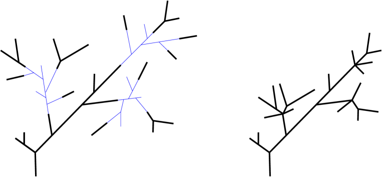
Figure 1: On the left side, the tree ${\mathcal{T}}$, with segments where $g$ is constant pictured in thin blue lines. On the right side, the subordinate tree, where each connected component of ${\mathcal{T}}$ made of thin segments has been glued into a single point.

Our main interest is in the case where ${\mathcal{T}}$ is random, and more precisely ${\mathcal{T}}={\mathcal{T}}_{\zeta}$ is the “Brownian tree” coded by a positive Brownian excursion $\zeta=(\zeta_{s})_{0\leq s\leq\sigma}$ under the Itô excursion measure. One may view ${\mathcal{T}}_{\zeta}$ as a variant of Aldous’ Brownian CRT, for which the total mass is not finite, but is distributed according to an infinite measure on $(0,\infty)$. As previously, we write $p_{\zeta}$ for the canonical projection from $[0,\sigma]$ onto ${\mathcal{T}}_{\zeta}$. Next, to define the subordination function, we let $(Z_{a})_{a\in{\mathcal{T}}_{\zeta}}$ be (linear) Brownian motion indexed by ${\mathcal{T}}_{\zeta}$, starting from $0$ at the root $\rho$. A simple way to construct this process is to use the Brownian snake approach, letting $Z_{a}=\widehat{W}_{s}$ if $a=p_{\zeta}(s)$, where $\widehat{W}_{s}$ is the “tip” of the random path $W_{s}$, which is the value at time $s$ of the Brownian snake driven by $\zeta$. Since $\zeta$ is distributed according to the Itô measure, $W$ follows the Brownian snake excursion measure away from $0$, which we denote by ${\mathbb{N}}_{0}$ (see [13, Chapter IV]). We then set $\overline{Z}_{a}=\max\{Z_{b}:b\in[[\rho,a]]\}$. In terms of the Brownian snake, we have $\overline{Z}_{a}=\overline{W}_{s}:=\max\{W_{s}(t):0\leq t\leq\zeta_{s}\}$ whenever $a=p_{\zeta}(s)$. We also use the notation $\underline{W}_{s}:=\min\{W_{s}(t):0\leq t\leq\zeta_{s}\}$.

Theorem 1.

Let $\widetilde{\mathcal{T}}_{\zeta}$ stand for the subordinate tree of ${\mathcal{T}}_{\zeta}$ with respect to the (continuous nondecreasing) function $a\mapsto\overline{Z}_{a}$. Under the Brownian snake excursion measure ${\mathbb{N}}_{0}$, the tree $\widetilde{\mathcal{T}}_{\zeta}$ is a Lévy tree with branching mechanism

$$\psi_{0}(r)=\sqrt{\frac{8}{3}}\,r^{3/2}.$$

Recall that Lévy trees represent the genealogy of continuous-state branching processes [8], and can be characterized by a regenerative property analogous to the branching property of Galton–Watson trees [23]. Our identification of the distribution of $\widetilde{\mathcal{T}}_{\zeta}$ is reminiscent of the classical result stating that the right-continuous inverse of the maximum process of a standard linear Brownian motion is a stable subordinator with index $1/2$.

In view of our applications, it turns out that it is important to have more information than the mere identification of $\widetilde{\mathcal{T}}_{\zeta}$ as a random compact ${\mathbb{R}}$-tree. As mentioned above, $\widetilde{\mathcal{T}}_{\zeta}$ can be viewed as the tree coded by the random function $s\mapsto\overline{Z}_{p_{\zeta}(s)}=\overline{W}_{s}$. This coding induces a “lexicographical” order structure on ${\mathcal{T}}_{\zeta}$ (see [6] for a thorough discussion of order structures on ${\mathbb{R}}$-trees). Somewhat surprisingly, it is not immediately clear that the order structure on $\widetilde{\mathcal{T}}_{\zeta}$ induced by the coding from the function $s\mapsto\overline{W}_{s}$ coincides with the usual order structure on Lévy trees, corresponding to the uniform random shuffling at every node in the terminology of [6]. To obtain this property, we relate the function $s\mapsto\overline{W}_{s}$ to the height process of [7, 8]. We recall that, from a Lévy process with Laplace exponent $\psi_{0}$, we can construct a continuous random process $(H_{t})_{t\geq 0}$ called the height process, which codes the $\psi_{0}$-Lévy tree (here and below we say $\psi_{0}$-Lévy tree rather than Lévy tree with branching mechanism $\psi_{0}$ for simplicity). See Section 3 below for more details.

Theorem 2.

There exists a process $H$, which is distributed under ${\mathbb{N}}_{0}$ as the height process of a Lévy tree with branching mechanism $\psi_{0}(r)=\sqrt{8/3}\,r^{3/2}$, and a continuous random process $\Gamma$ with nondecreasing sample paths, such that we have, ${\mathbb{N}}_{0}$ a.e. for every $s\geq 0$,

$$\overline{W}_{s}=H_{\Gamma_{s}}.$$

Both $H$ and $\Gamma$ will be constructed in the proof of Theorem 2, and are measurable functions of $(W_{s})_{s\geq 0}$. It is possible to identify the random process $\Gamma$ as a continuous additive functional of the Brownian snake, but we do not need this fact in the subsequent applications, and we do not discuss this matter in the present work.

Theorem 2 implies that the tree coded by $\overline{W}_{s}$ is isometric to the tree coded by $H_{s}$, and we recover Theorem 1. But Theorem 2 gives much more, namely that the order structure induced by the coding via $s\to\overline{W}_{s}$ is the same as the order structure induced by the usual height function of the Lévy tree. Order structures are crucial for our applications to the Brownian map. Similarly as in [19], we deal with a version of the Brownian map with randomized volume, which is constructed as a quotient space of the tree ${\mathcal{T}}_{\zeta}$: Two points $a$ and $b$ of ${\mathcal{T}}_{\zeta}$ are identified if $Z_{a}=Z_{b}$ and if $Z_{c}\geq Z_{a}$ for every $c\in[a,b]$, where $[a,b]$ is the set of all points that are visited when going from $a$ to $b$ around the tree in “clockwise” order (for this to make sense, it is essential that ${\mathcal{T}}_{\zeta}$ has been equipped with a lexicographical order structure). We write ${\bf m}$ for the resulting quotient space (the Brownian map) and $D^{*}$ for the metric on the Brownian map (see [15, 16] for more details). The space ${\bf m}$ comes with two distinguished points, namely the root $\rho$ of ${\mathcal{T}}_{\zeta}$ and the unique point $\rho_{*}$ where $Z$ attains its minimal value – in a sense that can be made precise, these two points are independent and uniformly distributed over ${\bf m}$. Let $B(r)$ be the closed ball of radius $r$ centered at $\rho_{*}$ in ${\bf m}$. For every $r\in(0,D(\rho^{*},\rho))$, define the hull $B^{\bullet}(r)$ as the complement of the connected component of the complement of $B(r)$ that contains $\rho$ (informally, $B^{\bullet}(r)$ is obtained by filling in all holes of $B(r)$ except for the one containing $\rho$). Following [19], we define the metric net $\mathcal{M}$ as the closure of

$$\bigcup_{0\leq r<D(\rho^{*},\rho)}\partial B^{\bullet}(r).$$

(This definition is in fact a little different from [19] which does not take the closure of the union in the last display.) We can equip the set $\mathcal{M}$ with an “intrinsic” metric $\Delta^{*}$ derived from the Brownian map metric $D^{*}$.

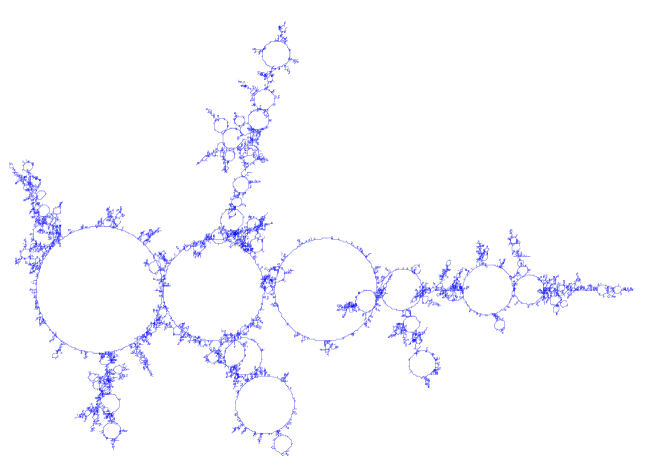
Figure 3: A simulation of a looptree (simulation by Igor Kortchemski). For technical reasons, some of the trees branching off a loop are pictured inside this loop, but, from the point of view of the present work, it is better to think of these trees as growing outside the loop, so that the space inside the loop may be “filled in” appropriately.

It is not hard to verify that, in the construction of ${\bf m}$ as a quotient space of ${\mathcal{T}}_{\zeta}$, points of $\mathcal{M}$ exactly correspond to vertices $a$ of ${\mathcal{T}}_{\zeta}$ such that $Z_{a}=\underline{Z}_{a}:=\min\{Z_{b}:b\in[[\rho,a]]\}$ (Proposition 10). This suggests that the metric net $\mathcal{M}$ is closely related to the subordinate tree of ${\mathcal{T}}_{\zeta}$ with respect to the function $a\mapsto-\underline{Z}_{a}$, which is a $\psi_{0}$-Lévy tree by the preceding results. To make this relation precise, we need the notion of the looptree introduced by Curien and Kortchemski [4] in a more general setting. Informally, the looptree associated with a Lévy tree is constructed by replacing each point $a$ of infinite multiplicity by a loop of “length” equal to the “weight” of $a$, in such a way that the subtrees that are the connected components of the complement of $a$ branch along this loop in an order determined by the coding function (see Fig.3 below for an illustration). To give a more precise definition, first note that Theorem 2 and an obvious symmetry argument allow us to find a process $(H^{\prime}_{s})_{s\geq 0}$ distributed as the height process of a $\psi_{0}$-Lévy tree, and a continuous random process $(\Gamma^{\prime}_{s})_{s\geq 0}$ with nondecreasing sample paths such that $-\underline{W}_{s}=H^{\prime}_{\Gamma^{\prime}_{s}}$. Then let $\chi:=\sup\{s\geq 0:H^{\prime}_{s}>0\}$, and let $\sim$ be the equivalence relation on $[0,\chi]$ whose graph is the smallest closed symmetric subset of $[0,\chi]^{2}$ that contains all pairs $(s,t)$ with $s\leq t$, $H^{\prime}_{s}=H^{\prime}_{t}$ and $H^{\prime}_{r}>H^{\prime}_{s}$ for every $r\in(s,t)$. The looptree ${\mathcal{L}}$ is defined as the quotient space $[0,\chi]/\sim$ equipped with an appropriate metric (see [4]). Clearly, $H^{\prime}_{\alpha}$ makes sense for any $\alpha\in{\mathcal{L}}$ and is interpreted as the height of $\alpha$. The metric on ${\mathcal{L}}$ is in fact not relevant for us, since we consider instead the pseudo-metric $\mathcal{D}^{\circ}$ defined for $\alpha,\beta\in{\mathcal{L}}$ by

$$\mathcal{D}^{\circ}(\alpha,\beta)=2\min\Bigg{(}\max_{\gamma\in[\alpha,\beta]}H^{\prime}_{\gamma},\max_{\gamma\in[\beta,\alpha]}H^{\prime}_{\gamma}\Bigg{)}-H^{\prime}_{\alpha}-H^{\prime}_{\beta},$$

where $[\alpha,\beta]$ corresponds to the subset of ${\mathcal{L}}$ visited when going from $\alpha$ to $\beta$ “around” ${\mathcal{L}}$ in “clockwise order” (see Section 7 for a more formal definition). We write $\alpha\simeq\beta$ if $\mathcal{D}^{\circ}(\alpha,\beta)=0$ (informally this means that $\alpha$ and $\beta$ “face each other” in the tree, in the sense that they are at the same height, and that points “between” $\alpha$ and $\beta$ are at a smaller height). It turns out that this defines an equivalence relation on ${\mathcal{L}}$. Finally, we let $\mathcal{D}^{*}$ be the largest symmetric function on ${\mathcal{L}}\times{\mathcal{L}}$ that is bounded above by $\mathcal{D}^{\circ}$ and satisfies the triangle inequality.

Theorem 3.

The metric net $(\mathcal{M},\Delta^{*})$ is a.s. isometric to the quotient space ${\mathcal{L}}/\!\simeq$ equipped with the metric induced by $\mathcal{D}^{*}$.

See Theorem 12 in Section 7 for a more precise formulation. Theorem 3 is closely related to Proposition 4.4 in [19], where, however, the metric net is not identified as a metric space. The description of the metric net is an important ingredient of the axiomatic characterization of the Brownian map discussed in [19].

Let us briefly comment on the motivations for studying the metric net. Roughly speaking, the Brownian map ${\bf m}$ can be recovered from the metric net $\mathcal{M}$ by filling in the “holes”. To make this precise, we observe that the connected components of ${\bf m}\backslash\mathcal{M}$ are bounded by Jordan curves (Proposition 14) and that these components are in one-to-one correspondence with connected components of ${\mathcal{T}}_{\zeta}\backslash\Theta$, where $\Theta:=\{a\in{\mathcal{T}}_{\zeta}:Z_{a}=\underline{Z}_{a}\}$. Each of the latter components is associated with an excursion of the Brownian snake above its minimum, in the terminology of [1], and the distribution of such an excursion only depends on its boundary size as defined in [1] (this boundary size can be interpreted as a generalized length of the Jordan curve bounding the corresponding component of ${\bf m}\backslash\mathcal{M}$). Theorem 40 in [1] shows that, conditionally on their boundary sizes, these excursions are independent and distributed according to a certain “excursion measure”. In the Brownian map setting, this means that the holes in the metric net are filled in independently, conditionally on the lengths of their boundaries.

The paper is organized as follows. Section 2 gives a brief discussion of subordination for deterministic trees, and Section 3 recalls the basic facts about Lévy trees that we need. After a short presentation of the Brownian snake, Section 4 gives the distribution of the subordinate tree $\widetilde{\mathcal{T}}_{\zeta}$ (Theorem 1). In view of identifying the order structure of this subordinate tree, Section 5 provides a technical result showing that the height process coding a Lévy tree is the limit in a strong sense of the discrete height functions coding embedded Galton–Watson trees. This result is related to the general limit theorems of [7, Chapter 2] proving that Lévy trees are weak limits of Galton–Watson trees, but the fact that we get a strong approximation is crucial for our applications. In Section 6, we prove that the Brownian snake maximum process $s\mapsto\overline{W}_{s}$ is a time change of the height process associated with a $\psi_{0}$-Lévy tree (Theorem 2). This result is a key ingredient of the developments of Section 7, where we identify the metric net of the Brownian map (Theorem 3). Section 8 discusses the connected components of the complement of the metric net, showing in particular that they are in one-to-one correspondence with the points of infinite multiplicity of the associated Lévy tree, and that the boundary of each component is a Jordan curve. Section 9, which is mostly independent of the preceding sections, discusses more general subordinations of the Brownian tree ${\mathcal{T}}_{\zeta}$, which lead to stable Lévy trees with an arbirary index. This section is related to our previous article [3], which dealt with subordination for spatial branching processes, but the latter work did not consider the associated genealogical structures as we do here, and the subordination method, based on the so-called residual lifetime process, was also different. Finally, the appendix presents a more general and more precise version of the special Markov property of the Brownian snake (first established in [12]), which plays an important role in several proofs.

2 Subordination of deterministic trees

In this short section, we present a few elementary considerations about deterministic ${\mathbb{R}}$-trees. We refer to [10] for the basic facts about ${\mathbb{R}}$-trees that we will need, and to [6] for a thorough study of the coding of compact ${\mathbb{R}}$-trees by functions.

Let us consider a compact ${\mathbb{R}}$-tree $({\mathcal{T}},d)$ rooted at $\rho$. If $a,b\in{\mathcal{T}}$, the geodesic segment between $a$ and $b$ (the range of the unique geodesic from $a$ to $b$) is denoted by $[[a,b]]$. The point $a\wedge b$ is then defined by $[[\rho,a\wedge b]]=[[\rho,a]]\cap[[\rho,b]]$. The genealogical partial order on ${\mathcal{T}}$ is denoted by $\prec\;$: we have $a\prec b$ if and only if $a\in[[\rho,b]]$, and we then say that $a$ is an ancestor of $b$, or $b$ is a descendant of $a$. Finally, the height of ${\mathcal{T}}$ is defined by

$$\mathcal{H}({\mathcal{T}})=\max_{a\in{\mathcal{T}}}d(\rho,a).$$

Let $g:{\mathcal{T}}\longrightarrow{\mathbb{R}}_{+}$ be a nonnegative continuous function on ${\mathcal{T}}$. Assume that $g(\rho)=0$ and that $g$ is nondecreasing with respect to the genealogical order ($a\prec b$ implies that $g(a)\leq g(b)$). We then define, for every $a,b\in{\mathcal{T}}$,

$$d^{(g)}(a,b)=g(a)+g(b)-2\,g(a\wedge b).$$

Notice that $d^{(g)}(a,b)$ is a symmetric function of $a$ and $b$ and satisfies the triangle inequality. We can thus consider the equivalence relation

$$a\approx_{g}b\quad\hbox{if and only if}\quad d^{(g)}(a,b)=0.$$

Thus $a\approx_{g}b$ if and only if $g(a)=g(b)=g(a\wedge b)$, and this is also equivalent to saying that $g(c)=g(a)$ for every $c\in[[a,b]]$. Write ${\mathcal{T}}^{(g)}$ for the quotient ${\mathcal{T}}/\!\approx_{g}$, and $\pi^{(g)}$ for the canonical projection from ${\mathcal{T}}$ onto ${\mathcal{T}}^{(g)}$.

Proposition 4.

The set ${\mathcal{T}}^{(g)}$ equipped with the distance induced by $d^{(g)}$ is again a compact ${\mathbb{R}}$-tree.

Proof.

One immediately verifies that, for every $a\in{\mathcal{T}}$, $\pi^{(g)}([[\rho,a]])$ is a segment in $({\mathcal{T}}^{(g)},d^{(g)})$ with endpoints $\pi^{(g)}(\rho)$ and $\pi^{(g)}(a)$. From Lemma 3.36 in [10], it then suffices to check that the four-point condition

$$d^{(g)}(a_{1},a_{2})+d^{(g)}(a_{3},a_{4})\leq\max\Big{(}d^{(g)}(a_{1},a_{3})+d^{(g)}(a_{2},a_{4}),d^{(g)}(a_{1},a_{4})+d^{(g)}(a_{2},a_{3})\Big{)}$$

holds for every $a_{1},a_{2},a_{3},a_{4}\in{\mathcal{T}}$. This is straightforward and we omit the details. ∎

We call $({\mathcal{T}}^{(g)},d^{(g)})$ the subordinate tree of $({\mathcal{T}},d)$ with respect to the function $g$. By convention, ${\mathcal{T}}^{(g)}$ is rooted at $\pi^{(g)}(\rho)$. Since $d^{(g)}(\rho,a)=g(a)$ for every $a\in{\mathcal{T}}$, we have $\mathcal{H}({\mathcal{T}}^{(g)})=\max\{g(a):a\in{\mathcal{T}}\}$.

Consider now a continuous function $h:[0,\sigma]\longrightarrow{\mathbb{R}}_{+}$, where $\sigma\geq 0$, such that $h(0)=h(\sigma)=0$, and assume that $({\mathcal{T}},d)$ is the tree coded by $h$ in the sense of [8] or [6]. This means that ${\mathcal{T}}={\mathcal{T}}_{h}$ is the quotient space $[0,\sigma]/\!\sim_{h}$, where the equivalence relation $\sim_{h}$ is defined on $[0,\sigma]$ by

$$s\sim_{h}t\quad\hbox{if and only if}\quad h(s)=h(t)=\min_{s\wedge t\leq r\leq r\vee t}h(r),$$

and $d=d_{h}$ is the distance induced on the quotient space by

$$d_{h}(s,t)=h(s)+h(t)-2\min_{s\wedge t\leq r\leq r\vee t}h(r).$$

Notice that the topology of $({\mathcal{T}}_{h},d_{h})$ coincides with the quotient topology on ${\mathcal{T}}_{h}$.

The canonical projection from $[0,\sigma]$ onto ${\mathcal{T}}_{h}$ is denoted by $p_{h}$, and ${\mathcal{T}}_{h}$ is rooted at $\rho_{h}=p_{h}(0)$. For $s\in[0,\sigma]$, the quantity $h(s)=d_{h}(0,s)$ is interpreted as the height of $p_{h}(s)$ in the tree. One easily verifies that, for every $s,t\in[0,\sigma]$, the property $p_{h}(s)\prec p_{h}(t)$ holds if and only if $h(s)=\min\{h(r):s\wedge t\leq r\leq s\vee t\}$.

Remark. The function $h$ is not determined by ${\mathcal{T}}_{h}$. In particular, if $\phi:[0,\sigma^{\prime}]\to[0,\sigma]$ is continuous and nondecreasing, and such that $\phi(0)=0$ and $\phi(\sigma^{\prime})=\sigma$, the tree coded by $h\circ\phi$ is isometric to the tree coded by $h$. This simple observation will be useful later.

Proposition 5.

Under the preceding assumptions, if $g$ is a nonnegative continuous function on ${\mathcal{T}}_{h}$ such that $g(\rho_{h})=0$ and $g$ is nondecreasing with respect to the genealogical order on ${\mathcal{T}}_{h}$, the subordinate tree $({\mathcal{T}}_{h}^{(g)},d_{h}^{(g)})$ of $({\mathcal{T}}_{h},d_{h})$ with respect to the function $g$ is isometric to the tree $({\mathcal{T}}_{G},d_{G})$ coded by the function $G=g\circ p_{h}$.

Proof.

Note that the function $G$ is nonnegative and continuous on $[0,\sigma]$, and $G(0)=G(\sigma)=0$. We can therefore make sense of the tree $({\mathcal{T}}_{G},d_{G})$ and as above we denote the canonical projection from $[0,\sigma]$ onto ${\mathcal{T}}_{G}$ by $p_{G}$. We first notice that, for every $s,t\in[0,\sigma]$, the property $p_{h}(s)=p_{h}(t)$ implies $p_{G}(s)=p_{G}(t)$. Indeed, if $p_{h}(s)=p_{h}(t)$, then, for every $r\in[s\wedge t,s\vee t]$, we have $p_{h}(s)\prec p_{h}(r)$ and therefore $g(p_{h}(s))\leq g(p_{h}(r))$, so that

$$G(s)=G(t)=\min_{r\in[s\wedge t,s\vee t]}G(r),$$

and $p_{G}(s)=p_{G}(t)$. We can thus write $p_{G}={\bf p}\circ p_{h}$, where the function ${\bf p}:{\mathcal{T}}_{h}\longrightarrow{\mathcal{T}}_{G}$ is continuous and onto.

Then, let $a,b\in{\mathcal{T}}_{h}$ and write $a=p_{h}(s)$ and $b=p_{h}(t)$, with $s,t\in[0,\sigma]$. We note that, for every $r\in[s\wedge t,s\vee t]$, $p_{h}(s)\wedge p_{h}(t)\prec p_{h}(r)$, and furthermore $p_{h}(s)\wedge p_{h}(t)=p_{h}(r_{0})$, if $r_{0}$ is any element of $[s\wedge t,s\vee t]$ at which $h$ attains its minimum over $[s\wedge t,s\vee t]$. It follows that

$$g(p_{h}(s)\wedge p_{h}(t))=\min_{r\in[s\wedge t,s\vee t]}G(r).$$

Hence,

$$d^{(g)}_{h}(a,b)=g(p_{h}(s))+g(p_{h}(t))-2g(p_{h}(s)\wedge p_{h}(t))=G(s)+G(t)-2\min_{r\in[s\wedge t,s\vee t]}G(r)=d_{G}(s,t).$$

If $\pi^{(g)}$ is the projection from ${\mathcal{T}}_{h}$ onto the subordinate tree ${\mathcal{T}}_{h}^{(g)}$, we see in particular that the condition $\pi^{(g)}(a)=\pi^{(g)}(b)$ implies $p_{G}(s)=p_{G}(t)$ and therefore ${\bf p}(a)={\bf p}(b)$.

It follows that ${\bf p}=I\circ\pi^{(g)}$, where $I:{\mathcal{T}}_{h}^{(g)}\longrightarrow{\mathcal{T}}_{G}$ is onto. It remains to verify that $I$ is isometric, but this is immediate from the identities in the last display. ∎

Remark. It is known that any compact ${\mathbb{R}}$-tree can be represented in the form ${\mathcal{T}}_{h}$ for some function $h$ (see [6, Corollary 1.2]). Thus Proposition 5 provides an alternative proof of Proposition 4.

3 Lévy trees

In the next sections, we will consider the case where ${\mathcal{T}}$ is the (random) tree coded by a Brownian excursion distributed under the Itô excursion measure ${\bf n}(\cdot)$, and we will identify certain subordinate trees as Lévy trees. In this section, we recall the basic facts about Lévy trees that will be needed later. We refer to [7, 8] for more details.

We consider a nonnegative function $\psi$ defined on $[0,\infty)$ of the type

$$\psi(r)=\alpha r+\beta r^{2}+\int_{(0,\infty)}\pi(\mathrm{d}u)\,(e^{-ur}-1+ur),$$ (1)

where $\alpha,\beta\geq 0$, and $\pi(\mathrm{d}u)$ is a $\sigma$-finite measure on $(0,\infty)$ such that $\int(u\wedge u^{2})\,\pi(\mathrm{d}u)<\infty$. With any such function $\psi$, we can associate a continuous-state branching process (see [11] and references therein), and $\psi$ is then called the branching mechanism function of this process. Notice that the conditions on $\psi$ are not the most general ones, because we restrict our attention to the critical or subcritical case. Additionally, we will assume that

$$\int_{1}^{\infty}\frac{\mathrm{d}r}{\psi(r)}<\infty.$$ (2)

This condition, which implies that at least one of the two properties $\beta>0$ or $\int u\,\pi(\mathrm{d}u)=\infty$ holds, is equivalent to the a.s. extinction of the continuous-state branching process with branching mechanism $\psi$ [11]. Special cases include $\psi(r)=r^{\gamma}$ for $1<\gamma\leq 2$.

Under the preceding assumptions, one can make sense of the Lévy tree that describes the genealogy of the continuous-state branching process with branching mechanism $\psi$. We consider, under a probability measure $\mathbf{P}$, a spectrally positive Lévy process $X=(X_{t})_{t\geq 0}$ with Laplace exponent $\psi$, meaning that $\mathbf{E}[\exp(-\lambda X_{t})]=\exp(t\psi(\lambda))$ for every $t\geq 0$ and $\lambda>0$. We define the associated height process by setting, for every $t\geq 0$,

$$H_{t}=\lim_{\varepsilon\to 0}\frac{1}{\varepsilon}\int_{0}^{t}\mathrm{d}s\,\mathbf{1}_{\{X_{s}<\inf\{X_{r}:s\leq r\leq t\}+\varepsilon\}}\,,$$

where the limit holds in probability under $\mathbf{P}$. Then [7, Theorem 1.4.3] the process $(H_{t})_{t\geq 0}$ has a continuous modification, which we consider from now on. We have $H_{t}=0$ if and only if $X_{t}=I_{t}$, where $I_{t}=\inf\{X_{s}:0\leq s\leq t\}$ is the past minimum process of $X$

Let $\mathbf{N}$ stand for the (infinite) excursion measure of $X-I$. Here the normalization of $\mathbf{N}$ is fixed by saying that the local time at $0$ of $X-I$ is the process $-I$. Let $\chi$ stand for the duration of the excursion under $\mathbf{N}$. The height process $H$ is well defined (and has continuous paths) under $\mathbf{N}$, and we have $H_{0}=H_{\chi}=0$, $\mathbf{N}$ a.e. To simplify notation, we will write $\max H=\max\{H_{s}:0\leq s\leq\chi\}$ under $\mathbf{N}$.

By definition (see [8, Definition 4.1]), the Lévy tree with branching mechanism $\psi$ (or in short the $\psi$-Lévy tree) is the random compact ${\mathbb{R}}$-tree ${\mathcal{T}}_{H}$ coded by the function $(H_{t})_{0\leq t\leq\chi}$ under $\mathbf{N}$, or more generally any random tree with the same distribution – note that the distribution of the Lévy tree is an infinite measure. We refer to [7, 8] for several results explaining in which sense the Lévy tree codes the genealogy of the continuous-state branching process with branching mechanism $\psi$. In the special case $\psi(r)=r^{2}/2$, $X$ is just a standard linear Brownian motion, $H_{t}=2(X_{t}-I_{t})$ is twice a reflected Brownian motion, and the Lévy tree is the tree coded by (twice) a positive Brownian excursion under the (suitably normalized) Itô measure. Conditioning on $\chi=1$ then yields the Brownian continuum random tree. When $\psi(r)=r^{\gamma}$ with $1<\gamma<2$, one gets the stable tree with index $\gamma$.

The distribution of the height of a Lévy tree is given as follows. For every $h>0$,

$$\mathbf{N}(\mathcal{H}({\mathcal{T}}_{H})>h)=\mathbf{N}(\max H>h)=v(h),$$

where the function $v:(0,\infty)\to(0,\infty)$ is determined by

$$\int_{v(h)}^{\infty}\frac{\mathrm{d}r}{\psi(r)}=h.$$

Remark. In the preceding considerations, the normalization of the infinite measure $\mathbf{N}$ is fixed by our choice of the local time at $0$ of $X-I$, and we can recover $\psi$ from $\mathbf{N}$ by the formulas for the distribution of $\mathcal{H}({\mathcal{T}}_{H})$ under $\mathbf{N}$. What happens if we multiply $\mathbf{N}$ by a constant $\lambda>0$ ? The tree ${\mathcal{T}}_{H}$ under $\lambda\mathbf{N}$ is still a Lévy tree in the previous sense, but the associated branching mechanism is now $\widetilde{\psi}(r)=\lambda\psi(r/\lambda)$. To see this, consider the Lévy process $X^{\prime}_{t}=\frac{1}{\lambda}X_{\lambda t}$, whose Laplace exponent is $\widetilde{\psi}(\lambda)$. It is not hard to verify that the height process corresponding to $X^{\prime}$ is $H^{\prime}_{t}=H_{\lambda t}$. Furthermore, if $\mathbf{N}^{\prime}$ is the excursion measure of $X^{\prime}$ above its past minimum process, one also checks that the distribution of $(H^{\prime}_{t/\lambda})_{t\geq 0}$ under $\mathbf{N}^{\prime}$ is the distribution of $(H_{t})_{t\geq 0}$ under $\lambda\mathbf{N}$. However, the tree coded by $(H^{\prime}_{t/\lambda})_{t\geq 0}$ is the same as the tree coded by $(H^{\prime}_{t})_{t\geq 0}$. This shows that ${\mathcal{T}}_{H}$ under $\lambda\mathbf{N}$ is a Lévy tree with branching mechanism $\widetilde{\psi}$. Note that this is consistent with the formula for $\mathbf{N}(\mathcal{H}({\mathcal{T}}_{H})>h)$.

We now state two results that will be important for our purposes. We first mention that, for every $h\geq 0$, one can define under $\mathbf{P}$ a local time process of $H$ at level $h$, which is denoted by $(L^{h}_{t})_{t\geq 0}$ and is such that the following approximation holds for every $t>0$,

$$\lim_{\varepsilon\to 0}\mathbf{E}\Big{[}\sup_{s\leq t}\Big{|}\frac{1}{\varepsilon}\int_{0}^{s}\mathbf{1}_{\{h<H_{s}\leq h+\varepsilon\}}\mathrm{d}r-L^{h}_{s}\Big{|}\Big{]}=0\,,$$ (3)

and the latter convergence is uniform in $h$ (see [7, Proposition 1.3.3]). When $h=0$ we have simply $L^{0}_{t}=-I_{t}$. The definition of $(L^{h}_{t})_{t\geq 0}$ also makes sense under $\mathbf{N}$, with a similar approximation.

We fix $h>0$, and let $(u_{j},v_{j})_{j\in J}$ be the collection of all excursion intervals of $H$ above level $h$: these are all intervals $(u,v)$, with $0\leq u<v$, such that $H_{u}=H_{v}=h$ and $H_{r}>h$ for every $r\in(u,v)$. For each such excursion interval $(u_{j},v_{j})$, we define the corresponding excursion by $H^{(j)}_{s}=H_{(u_{j}+s)\wedge v_{j}}-h$, for every $s\geq 0$. Then $H^{(j)}$ is a random element of the space $C({\mathbb{R}}_{+},{\mathbb{R}}_{+})$ of all continuous functions from ${\mathbb{R}}_{+}$ into ${\mathbb{R}}_{+}$. We also let $\mathbf{N}^{\circ}$ be the $\sigma$-finite measure on $C({\mathbb{R}}_{+},{\mathbb{R}}_{+})$ which is the “law” of $(H_{s})_{s\geq 0}$ under $\mathbf{N}$.

Proposition 6.

(i) Under the probability measure $\mathbf{P}$, the point measure

$$\sum_{j\in J}\delta_{(L^{h}_{u_{j}},H^{(j)})}(\mathrm{d}\ell,\mathrm{d}\omega)$$

is Poisson with intensity $\mathbf{1}_{[0,\infty)}(\ell)\,\mathrm{d}\ell\,\mathbf{N}^{\circ}(\mathrm{d}\omega)$.

(ii) Under the probability measure $\mathbf{N}(\cdot\mid\max H>h)$ and conditionally on $L^{h}_{\chi}$, the point measure

$$\sum_{j\in J}\delta_{(L^{h}_{u_{j}},H^{(j)})}(\mathrm{d}\ell,\mathrm{d}\omega)$$

is Poisson with intensity $\mathbf{1}_{[0,L^{h}_{\chi}]}(\ell)\,\mathrm{d}\ell\,\mathbf{N}^{\circ}(\mathrm{d}\omega)$.

See [8, Proposition 3.1, Corollary 3.2] for a slightly more precise version of this proposition. It follows from the preceding proposition that Lévy trees satisfy a branching property analogous to the classical branching property of Galton–Watson trees. To state this property, we introduce some notation. If $({\mathcal{T}},d)$ is a (deterministic) compact ${\mathbb{R}}$-tree and $0<h<\mathcal{H}({\mathcal{T}})$, we can consider the subtrees of ${\mathcal{T}}$ above level $h$. Here, a subtree above level $h$ is just the closure of a connected component of $\{a\in{\mathcal{T}}:d(\rho,a)>h\}$. Such a subtree is itself viewed as a rooted ${\mathbb{R}}$-tree (the root is obviously the unique point at height $h$ in the subtree).

Proposition 7.

Let ${\mathcal{T}}$ be a random compact ${\mathbb{R}}$-tree defined under an infinite measure $\mathcal{N}$, such that $\mathcal{N}(\mathcal{H}({\mathcal{T}})=0)=0$ and $0<\mathcal{N}(\mathcal{H}({\mathcal{T}})>h)<\infty$ for every $h>0$. For every $h,\varepsilon>0$, write $M(h,h+\varepsilon)$ for the number of subtrees of ${\mathcal{T}}$ above level $h$ with height greater than $\varepsilon$.

1. Suppose that ${\mathcal{T}}$ is a Lévy tree. Then, for every $h,\varepsilon>0$, for every integer $p\geq 1$, the distribution under $\mathcal{N}(\cdot\mid M(h,h+\varepsilon)=p)$ of the unordered collection formed by the $p$ subtrees of ${\mathcal{T}}$ above level $h$ with height greater than $\varepsilon$ is the same as that of the unordered collection of $p$ independent copies of ${\mathcal{T}}$ under $\mathcal{N}(\cdot\mid\mathcal{H}({\mathcal{T}})>\varepsilon)$.

2. Conversely, if the property stated in (i) holds, then ${\mathcal{T}}$ is a Lévy tree.

The property stated in (i) is called the branching property. The fact that it holds for Lévy trees is a straightforward consequence of Proposition 6 (ii). For the converse, we refer to [23, Theorem 1.1]. Note that the branching property remains valid if we multiply the underlying measure $\mathcal{N}$ by a positive constant, which is consistent with the remark above.

To conclude this section, let us briefly comment on points of infinite multiplicity of the Lévy tree ${\mathcal{T}}_{H}$. The multiplicity of a point $a$ of ${\mathcal{T}}_{H}$ is the number of connected components of ${\mathcal{T}}_{H}\backslash\{a\}$, and $a$ is called a leaf if it has multiplicity one. Suppose that there is no quadratic part in $\psi$, meaning that the constant $\beta$ in (1) is $0$ (note that condition (2) then implies that $\pi$ has infinite mass). Then [8, Theorem 4.6], all points of ${\mathcal{T}}_{H}$ have multiplicity $1$, $2$ or $\infty$. The set of all points of infinite multiplicity is a countable dense subset of ${\mathcal{T}}_{H}$, and these points are in one-to-one correspondence with local minima of $H$, or with jump times of $X$. More precisely, let $a$ be a point of infinite multiplicity of ${\mathcal{T}}_{H}$. Then, if $s_{1}=\min p_{H}^{-1}(a)$ and $s_{2}=\max p_{H}^{-1}(a)$, we have $s_{1}<s_{2}$, $H_{s_{1}}=H_{s_{2}}=\min\{H_{s}:s_{1}\leq s\leq s_{2}\}$, and $p_{H}^{-1}(a)=\{s\in[s_{1},s_{2}]:H_{s}=H_{s_{1}}\}$ is a Cantor set contained in $[s_{1},s_{2}]$. In terms of the Lévy process $X$, $s_{1}$ is a jump time of $X$ and $s_{2}=\inf\{s\geq s_{1}:X_{s}\leq X_{s_{1}-}\}$, and $p_{H}^{-1}(a)$ consists exactly of those $s\in[s_{1},s_{2}]$ such that $\inf\{X_{r}:r\in[s_{1},s]\}=X_{s}$. Furthermore, if for every $r\in[0,\Delta X_{s_{1}}]$ we set $\eta_{r}=\inf\{s\geq s_{1}:X_{s}<X_{s_{1}}-r\}$, the points of $p_{H}^{-1}(a)$ are all of the form $\eta_{r}$ or $\eta_{r-}$. The quantity $\Delta X_{s_{1}}$ is the “weight” of the point of infinite multiplicity $a$. See [8] for more details.

4 Subordination by the Brownian snake maximum

In this section, we prove Theorem 1. We start with a brief presentation of the Brownian snake. We refer to [13, Chapter IV] for more details.

We let $\mathcal{W}$ be the space of all finite paths in ${\mathbb{R}}$. Here a finite path is simply a continuous mapping $\mathrm{w}:[0,\zeta]\longrightarrow{\mathbb{R}}$, where $\zeta=\zeta_{(\mathrm{w})}$ is a nonnegative real number called the lifetime of $\mathrm{w}$. The set $\mathcal{W}$ is a Polish space when equipped with the distance

$$d_{\mathcal{W}}(\mathrm{w},\mathrm{w}^{\prime})=|\zeta_{(\mathrm{w})}-\zeta_{(\mathrm{w}^{\prime})}|+\sup_{t\geq 0}|\mathrm{w}(t\wedge\zeta_{(\mathrm{w})})-\mathrm{w}^{\prime}(t\wedge\zeta_{(\mathrm{w}^{\prime})})|.$$

The endpoint (or tip) of the path $\mathrm{w}$ is denoted by $\widehat{\mathrm{w}}=\mathrm{w}(\zeta_{(\mathrm{w})})$. For every $x\in{\mathbb{R}}$, we set $\mathcal{W}_{x}=\{\mathrm{w}\in\mathcal{W}:\mathrm{w}(0)=x\}$. We also identify the trivial path of $\mathcal{W}_{x}$ with zero lifetime with the point $x$.

The standard (one-dimensional) Brownian snake with initial point $x$ is the continuous Markov process $(W_{s})_{s\geq 0}$ taking values in $\mathcal{W}_{x}$, whose distribution is characterized by the following properties:

1. The process $(\zeta_{(W_{s})})_{s\geq 0}$ is a reflected Brownian motion in ${\mathbb{R}}_{+}$ started from $0$. To simplify notation, we write $\zeta_{s}=\zeta_{(W_{s})}$ for every $s\geq 0$.

2. Conditionally on $(\zeta_{s})_{s\geq 0}$, the process $(W_{s})_{s\geq 0}$ is time-inhomogeneous Markov, and its transition kernels are specified as follows. If $0\leq s\leq s^{\prime}$,

   1. $W_{s^{\prime}}(t)=W_{s}(t)$ for every $t\leq m_{\zeta}(s,s^{\prime}):=\min\{\zeta_{r}:s\leq r\leq s^{\prime}\}$;

   2. the random path $(W_{s^{\prime}}(m_{\zeta}(s,s^{\prime})+t)-W_{s^{\prime}}(m_{\zeta}(s,s^{\prime})))_{0\leq t\leq\zeta_{s^{\prime}}-m_{\zeta}(s,s^{\prime})}$ is independent of $W_{s}$ and distributed as a real Brownian motion started at $0$ and stopped at time $\zeta_{s^{\prime}}-m_{\zeta}(s,s^{\prime})$.

Informally, the value $W_{s}$ of the Brownian snake at time $s$ is a one-dimensional Brownian path started from $x$, with lifetime $\zeta_{s}$. As $s$ varies, the lifetime $\zeta_{s}$ evolves like reflected Brownian motion in ${\mathbb{R}}_{+}$. When $\zeta_{s}$ decreases, the path is erased from its tip, and when $\zeta_{s}$ increases, the path is extended by adding “little pieces” of Brownian paths at its tip.

For every $x\in{\mathbb{R}}$, we write ${\mathbb{P}}_{x}$ for the probability measure under which $W_{0}=x$, and ${\mathbb{N}}_{x}$ for the (infinite) excursion measure of $W$ away from $x$. Also $\sigma:=\sup\{s>0:\zeta_{s}>0\}$ stands for the duration of the excursion under ${\mathbb{N}}_{x}$. Under ${\mathbb{N}}_{x}$, $(\zeta_{s})_{s\geq 0}$ is distributed according to the Itô excursion measure ${\bf n}(\cdot)$, and the normalization is fixed by the formula

$${\mathbb{N}}_{x}\Big{(}\max_{0\leq s\leq\sigma}\zeta_{s}>\varepsilon\Big{)}=\frac{1}{2\varepsilon}.$$

The following property of the Brownian snake will be used in several places below. Recall that $\widehat{W}_{s}=W_{s}(\zeta_{s})$ is the tip of the path $W_{s}$. We say that $r\in[0,\sigma)$ is a time of right increase of $s\mapsto\zeta_{s}$, resp. of $s\mapsto\widehat{W}_{s}$, if there exists $\varepsilon\in(0,\sigma-r]$ such that $\zeta_{u}\geq\zeta_{r}$, resp. $\widehat{W}_{u}\geq\widehat{W}_{r}$, for every $u\in[r,r+\varepsilon]$. We can similarly define points of left increase. Then according to [17, Lemma 3.2], ${\mathbb{N}}_{x}$ a.e., no time $r\in(0,\sigma)$ can be simultaneously a time of (left or right) increase of $s\mapsto\zeta_{s}$ and a point of (left or right) increase of $s\mapsto\widehat{W}_{s}$.

Le us fix $x=0$ and argue under ${\mathbb{N}}_{0}$. As previously, we write ${\mathcal{T}}_{\zeta}$ for the (random) tree coded by the function $(\zeta_{s})_{0\leq s\leq\sigma}$, $p_{\zeta}:[0,\sigma]\longrightarrow{\mathcal{T}}_{\zeta}$ for the canonical projection, and $\rho_{\zeta}=p_{\zeta}(0)$ for the root of ${\mathcal{T}}_{\zeta}$. Properties of the Brownian snake show that the condition $p_{\zeta}(s)=p_{\zeta}(s^{\prime})$ implies $W_{s}=W_{s^{\prime}}$, and thus we can define $W_{a}$ for every $a\in{\mathcal{T}}_{\zeta}$ by setting $W_{a}=W_{s}$ if $a=p_{\zeta}(s)$. We note that, if $a=p_{\zeta}(s)$ and $t\in[0,\zeta_{s}]$, $W_{s}(t)$ coincides with $\widehat{W}_{b}$ where $b$ is the unique point of $[[\rho_{\zeta},a]]$ at distance $t$ from $\rho_{\zeta}$. For every $\mathrm{w}\in\mathcal{W}$, set

$$\overline{\mathrm{w}}:=\max_{0\leq t\leq\zeta_{(\mathrm{w})}}\mathrm{w}(t).$$

Then, the function $a\mapsto\overline{W}_{a}$ is continuous and nondecreasing on ${\mathcal{T}}_{\zeta}$ (if $a=p_{\zeta}(s)$ and $b=p_{\zeta}(s^{\prime})$, the condition $a\prec b$ implies that $\zeta_{s}\leq\zeta_{s^{\prime}}$ and that $W_{a}$ is the restriction of $W_{b}$ to the interval $[0,\zeta_{s}]$, so that obviously $\overline{W}_{a}\leq\overline{W}_{b}$). As in Theorem 1, we write $\widetilde{\mathcal{T}}_{\zeta}$ for the subordinate tree of ${\mathcal{T}}_{\zeta}$ with respect to the function $a\mapsto\overline{W}_{a}$.

Proof of Theorem 1. We first verify that the branching property stated in Proposition 7 holds for $\widetilde{\mathcal{T}}_{\zeta}$ under ${\mathbb{N}}_{0}$, and to this end we rely on the special Markov property of the Brownian snake.

Let $h>0$, and, for every $\mathrm{w}\in\mathcal{W}$, set $\tau_{h}(\mathrm{w})=\inf\{t\in[0,\zeta_{(\mathrm{w})}]:\mathrm{w}(t)\geq h\}$. Let $(a_{i},b_{i})_{i\in I}$ be the connected components of the open set $\{s\geq 0:\tau_{h}(W_{s})<\zeta_{s}\}$. For every such connected component $(a_{i},b_{i})$, for every $s\in[a_{i},b_{i}]$, the path $W_{s}$ coincides with $W_{a_{i}}=W_{b_{i}}$ up to time $\tau_{h}(W_{a_{i}})=\zeta_{a_{i}}=\zeta_{b_{i}}=\tau_{h}(W_{b_{i}})$ (these assertions are straightforward consequences of the properties of the Brownian snake, and we omit the details). We then set, for every $s\geq 0$,

$$W^{(i)}_{s}(t):=W_{(a_{i}+s)\wedge b_{i}}(\zeta_{a_{i}}+t),\quad\hbox{for }0\leq t\leq\zeta^{(i)}_{s}:=\zeta_{(a_{i}+s)\wedge b_{i}}-\zeta_{a_{i}}.$$

We view $W^{(i)}$ as a random element of the space of all continuous functions from ${\mathbb{R}}_{+}$ into $\mathcal{W}_{h}$, and the $W^{(i)}$’s are called the excursions of $W$ outside the domain $(-\infty,h)$ (see the appendix below for further details in a more general setting).

By a compactness argument, only finitely many of the excursions $W^{(i)}$ hit $(h+\varepsilon,\infty)$. Let $M_{h,\varepsilon}$ be the number of these excursions. It follows from Corollary 22 in the appendix that, for every $p\geq 1$, conditionally on $\{M_{h,\varepsilon}=p\}$, the unordered collection formed by the excursions of $W$ outside $(-\infty,h)$ that hit $(h+\varepsilon,\infty)$ is distributed as the unordered collection of $p$ independent copies of $W$ under ${\mathbb{N}}_{h}(\cdot\mid\sup\{\widehat{W}_{s}:s\geq 0\}>h+\varepsilon)$. On the other hand, noting that $\widetilde{\mathcal{T}}_{\zeta}$ is the tree coded by the function $[0,\sigma]\ni s\mapsto\overline{W}_{s}$ (by Proposition 5), we also see that subtrees of $\widetilde{\mathcal{T}}_{\zeta}$ above level $h$ with height greater than $\varepsilon$ are in one-to-one correspondence with excursions of $W$ outside $(-\infty,h)$ that hit $(h+\varepsilon,\infty)$, and if a subtree $\widetilde{\mathcal{T}}^{(i)}$ corresponds to an excursion $W^{(i)}$, $\widetilde{\mathcal{T}}^{(i)}$ is obtained from the excursion $W^{(i)}$ (shifted so that it starts from $0$) by exactly the same procedure that allows us to construct $\widetilde{\mathcal{T}}_{\zeta}$ from $W$ under ${\mathbb{N}}_{0}$: To be specific, $\widetilde{\mathcal{T}}^{(i)}$ is coded by the function $s\mapsto\overline{W}^{(i)}_{s}-h$ just as $\widetilde{\mathcal{T}}_{\zeta}$ is coded by $s\mapsto\overline{W}_{s}$. The preceding considerations show that $\widetilde{\mathcal{T}}_{\zeta}$ satisfies the branching property, and therefore is a Lévy tree.

To get the formula for $\psi_{0}$, we note that the distribution of the height of $\widetilde{\mathcal{T}}_{\zeta}$ is given by

$${\mathbb{N}}_{0}(\mathcal{H}(\widetilde{\mathcal{T}}_{\zeta})>r)={\mathbb{N}}_{0}\Big{(}\sup_{s\geq 0}\widehat{W}_{s}>r\Big{)}=\frac{3}{2r^{2}},$$

where the last equality can be found in [13, Section VI.1]. Since we also know that the function $v(r)={\mathbb{N}}_{0}(\mathcal{H}(\widetilde{\mathcal{T}}_{\zeta})>r)$ solves $v^{\prime}=-\psi_{0}(v(r))$, the formula for $\psi_{0}$ follows. $\square$

5 Approximating a Lévy tree by embedded Galton–Watson trees

In this section, we come back to the general setting of Section 3. Our goal is to prove that the Lévy tree ${\mathcal{T}}_{H}$ is (under the probability measure $\mathbf{N}(\cdot\mid\mathcal{H}({\mathcal{T}}_{H})>h)$ for some $h>0$) the almost sure limit of a sequence of embedded Galton–Watson trees, and that this limit is consistent with the order structure of the Lévy tree. We refer to [14] for basic facts about Galton–Watson trees. A key property for us is the fact that Galton–Watson trees are rooted ordered (discrete) trees, also called plane trees, so that there is a lexicographical ordering on vertices.

In what follows, we argue under the probability measure $\mathbf{P}$. Recall that $X$ is under $\mathbf{P}$ a Lévy process with Laplace exponent $\psi$, and that $H$ is the associated height process. We fix an integer $n\geq 1$, and, for every integer $j\geq 0$, we consider the sequence of all excursions of $H$ above level $j\,2^{-n}$ that hit level $(j+1)2^{-n}$. We let

$$0\leq\alpha^{n}_{0}<\alpha^{n}_{1}<\alpha^{n}_{2}<\cdots$$

be the ordered sequence consisting of all the initial times of these excursions, for all values of the integer $j\geq 0$ (so, $\alpha^{n}_{0}$ corresponds to the beginning of an excursion of $H$ above $0$ that hits $2^{-n}$, $\alpha^{n}_{1}$ may be either the beginning of an excursion of $H$ above $0$ that hits $2^{-n}$ or the beginning of an excursion of $H$ above $2^{-n}$ that hits $2\times 2^{-n}$, and so on). For every $j\geq 0$, we also let $\beta^{n}_{j}$ be the terminal time of the excursion starting at time $\alpha^{n}_{j}$.

We then set, for every integer $k\geq 0$,

$$H^{n}_{k}=2^{n}\,H_{\alpha^{n}_{k}}.$$

Proposition 8.

The process $(H^{n}_{k})_{k\geq 0}$ is the discrete height process of a sequence of independent Galton–Watson trees with the same offspring distribution $\mu_{n}$.

Recall that the discrete height process of a sequence of Galton–Watson trees gives the generation of the successive vertices in the trees, assuming that these vertices are listed in lexicographical order in each tree and one tree after another. See [14] or [7, Section 0.2]. The (finite) height sequence of a single tree is defined analogously.

Proof.

By construction, $\alpha^{n}_{0}$ is the initial time of the first excursion of $H$ above $0$ that hits $2^{-n}$. Notice that this excursion is distributed as $H$ under ${\bf N}(\cdot\mid\max H\geq 2^{-n})$. Let $K\geq 1$ be the (random) integer such that $\alpha^{n}_{K-1}<\beta^{n}_{0}\leq\alpha^{n}_{K}$, so that $\alpha^{n}_{K}$ is the initial time of the second excursion of $H$ above $0$ that hits $2^{-n}$.

With the excursion of $H$ during interval $[\alpha^{n}_{0},\beta^{n}_{0}]$, we can associate a (plane) tree ${\mathcal{T}}^{n}_{0}$ constructed as follows. The children of the ancestor correspond to the excursions of $H$ above level $2^{-n}$, during the time interval $[\alpha^{n}_{0},\beta^{n}_{0}]$, that hit $2\times 2^{-n}$ and the order on these children is obviously given by the chronological order. Equivalently, the children of the ancestor correspond to the indices $i\in\{1,\ldots,K-1\}$ such that $H^{n}_{i}=1$. Then, assuming that the ancestor has at least one child (equivalently that $K\geq 2$), the children of the first child of the ancestor correspond to the excursions of $H$ above level $2\times 2^{-n}$, during the time interval $[\alpha^{n}_{1},\beta^{n}_{1}]$, that hit $3\times 2^{-n}$, and so on. See Fig.2 for an illustration.

Figure 2: The sequence $\alpha^{n}_{0},\alpha^{n}_{1},\ldots$ and the tree ${\mathcal{T}}^{n}_{0}$ (in thick lines).

Write $N^{n}_{0}$ for the number of children of the ancestor in ${\mathcal{T}}^{n}_{0}$. It follows from Proposition 6 (ii) that, conditionally on $N^{n}_{0}$, the successive excursions of $H$ above level $2^{-n}$, during the time interval $[\alpha^{n}_{0},\beta^{n}_{0}]$, that hit $2\times 2^{-n}$ are independent and distributed as $H$ under ${\bf N}(\cdot\mid\max H\geq 2^{-n})$ (recall that our definition shifts excursions above a level $h$ so that they start from $0$). Recalling the construction of the tree ${\mathcal{T}}^{n}_{0}$, we now obtain that, conditionally on $N^{n}_{0}$, the subtrees of ${\mathcal{T}}^{n}_{0}$ originating from the children of the ancestor are independent and distributed according to ${\mathcal{T}}^{n}_{0}$. This just means that ${\mathcal{T}}^{n}_{0}$ is a Galton–Watson tree, and its offspring distribution $\mu_{n}$ is the law under ${\bf N}(\cdot\mid\max H\geq 2^{-n})$ of the number of excursions of $H$ above level $2^{-n}$ that hit $2\times 2^{-n}$.

With the second excursion of $H$ above $0$ that hits $2^{-n}$, we can similarly associate a Galton–Watson tree ${\mathcal{T}}^{n}_{1}$ with offspring distribution $\mu_{n}$, and so on. The trees ${\mathcal{T}}^{n}_{0},{\mathcal{T}}^{n}_{1},\ldots$ are independent as a consequence of the strong Markov property of the Lévy process $X$. By construction, the process $(H^{n}_{k})_{k\geq 0}$ is the discrete height process of the sequence ${\mathcal{T}}^{n}_{0},{\mathcal{T}}^{n}_{1},\ldots$. ∎

Proposition 9.

For every $n\geq 1$, set $v_{n}:=2^{n}v(2^{-n})=2^{n}{\bf N}(\max H\geq 2^{-n})$. Then, for every $A>0$,

$$\sup_{t\leq A}|2^{-n}H^{n}_{\lfloor v_{n}t\rfloor}-H_{t}|\mathrel{\mathop{\kern 0.0pt\longrightarrow}\limits_{n\to\infty}}0$$

in probability under $\mathbf{P}$.

Proof.

Recall that, for every $h\geq 0$, $(L^{h}_{t})_{t\geq 0}$ denotes the local time of $H$ at level $h$. It will be convenient to introduce, for every $n\geq 1$ and every $j\geq 0$, the increasing process

$$\mathcal{N}^{n}_{(j)}(t):=\#\{k\geq 0:H^{n}_{k}=j,L^{j2^{-n}}_{\alpha^{n}_{k}}\leq t\}.$$

As a consequence of Proposition 6(i) applied with $h=j2^{-n}$, we get that $\mathcal{N}^{n}_{(j)}(t)$ is a Poisson process with parameter $v(2^{-n})={\bf N}(\max H\geq 2^{-n})$.

We claim that, for every $A>0$,

$$\lim_{n\to\infty}\sup_{j\geq 0}\Bigg{(}\mathbf{E}\Big{[}\sup_{s\leq A}|v(2^{-n})^{-1}\,\#\{k:H^{n}_{k}=j,\alpha^{n}_{k}\leq s\}-L^{j2^{-n}}_{s}|\Big{]}\Bigg{)}=0.$$ (4)

To see this, first observe that, for every $s>0$,

$$\mathcal{N}^{n}_{(j)}((L_{s}^{j2^{-n}})-)\leq\#\{k:H^{n}_{k}=j,\alpha^{n}_{k}\leq s\}\leq\mathcal{N}^{n}_{(j)}(L_{s}^{j2^{-n}}),$$

and then write

$$\mathbf{E}\Big{[}\sup_{s\leq A}|v(2^{-n})^{-1}\,\#\{k:H^{n}_{k}=j,\alpha^{n}_{k}\leq s\}-L^{j2^{-n}}_{s}|\Big{]}$$

$$\qquad\leq\sum_{p=1}^{\infty}\mathbf{E}\Big{[}\mathbf{1}_{\{p-1\leq L^{j2^{-n}}_{A}\leq p\}}\sup_{t\leq p}|v(2^{-n})^{-1}\,\mathcal{N}^{n}_{(j)}(t)-t|\Big{]}$$

$$\qquad\leq\sum_{p=1}^{\infty}\mathbf{P}(p-1\leq L^{j2^{-n}}_{A})^{1/2}\,\mathbf{E}\Big{[}\sup_{t\leq p}|v(2^{-n})^{-1}\,\mathcal{N}^{n}_{(j)}(t)-t|^{2}\Big{]}^{1/2}.$$

Then, if $\mathcal{N}(t)$ stands for a standard Poisson process, we have by a classical martingale inequality

$$\mathbf{E}\Big{[}\sup_{t\leq p}|v(2^{-n})^{-1}\,\mathcal{N}^{n}_{(j)}(t)-t|^{2}\Big{]} =v(2^{-n})^{-2}\mathbf{E}\Big{[}\sup_{t\leq v(2^{-n})p}(\mathcal{N}(t)-t)^{2}\Big{]}$$

$$\leq 4v(2^{-n})^{-2}\,\mathbf{E}[(\mathcal{N}(v(2^{-n})p)-v(2^{-n})p)^{2}]$$

$$=4v(2^{-n})^{-1}p.$$

It follows that, for every $j\geq 0$,

$$\mathbf{E}\Big{[}\sup_{s\leq A}|v(2^{-n})^{-1}\,\#\{k:H^{n}_{k}=j,\alpha^{n}_{k}\leq s\}-L^{j2^{-n}}_{s}|\Big{]}\leq\Big{(}\sum_{p=1}^{\infty}(p\,\mathbf{P}(p-1\leq L^{j2^{-n}}_{A}))^{1/2}\Big{)}\times 2v(2^{-n})^{-1/2},$$

and the proof of (4) is completed by noting that $v(2^{-n})\longrightarrow\infty$ as $n\to\infty$, and that

$$\sum_{p=1}^{\infty}(p\,\mathbf{P}(p-1\leq L^{j2^{-n}}_{A}))^{1/2}\leq\sum_{p=1}^{\infty}(p\,\mathbf{P}(p-1\leq L^{0}_{A}))^{1/2}<\infty,$$

because $L^{j2^{-n}}_{A}$ is bounded above in distribution by $L^{0}_{A}$ (cf Definition 1.3.1 in [7]), and we know that $L^{0}_{A}=-I_{A}$ has exponential moments..

Let $\ell\geq 1$ be an integer. By summing the convergence in (4) over possible choices of $0\leq j<\ell 2^{n}$, we also obtain that

$$\lim_{n\to\infty}\mathbf{E}\Big{[}\sup_{s\leq A}\Big{|}2^{-n}v(2^{-n})^{-1}\,\#\{k:H_{\alpha^{n}_{k}}<\ell,\alpha^{n}_{k}\leq s\}-2^{-n}\sum_{j=0}^{\ell 2^{n}-1}L^{j2^{-n}}_{s}\Big{|}\Big{]}=0.$$ (5)

On the other hand, we have, for every $s\geq 0$,

$$\Big{|}\int_{0}^{s}\mathrm{d}r\,\mathbf{1}_{\{H_{r}\leq\ell\}}-2^{-n}\sum_{j=0}^{\ell 2^{n}-1}L^{j2^{-n}}_{s}\Big{|} =\Big{|}\sum_{j=0}^{\ell 2^{n}-1}\Big{(}\int_{0}^{s}\mathrm{d}r\,\mathbf{1}_{\{j2^{-n}<H_{r}\leq(j+1)2^{-n}\}}-2^{-n}L^{j2^{-n}}_{s}\Big{)}\Big{|}$$

$$\leq 2^{-n}\sum_{j=0}^{\ell 2^{n}-1}\Big{|}2^{n}\int_{0}^{s}\mathrm{d}r\,\mathbf{1}_{\{j2^{-n}<H_{r}\leq(j+1)2^{-n}\}}-L^{j2^{-n}}_{s}\Big{|},$$

and it follows from (3) that

$$\lim_{n\to\infty}\mathbf{E}\Big{[}\sup_{s\leq A}\Big{|}\int_{0}^{s}\mathrm{d}r\,\mathbf{1}_{\{H_{r}\leq\ell\}}-2^{-n}\sum_{j=0}^{\ell 2^{n}-1}L^{j2^{-n}}_{s}\Big{|}\Big{]}=0.$$ (6)

By combining (5) and (6), we get

$$\lim_{n\to\infty}\mathbf{E}\Big{[}\sup_{s\leq A}\Big{|}\int_{0}^{s}\mathrm{d}r\,\mathbf{1}_{\{H_{r}\leq\ell\}}-v_{n}^{-1}\,\#\{k:H_{\alpha^{n}_{k}}<\ell,\alpha^{n}_{k}\leq s\}\Big{|}\Big{]}=0,$$

where $v_{n}=2^{n}v(2^{-n})$. Since $\mathbf{P}(\max\{H_{s}:0\leq s\leq A\}\geq\ell)$ can be made arbitrarily small by choosing $\ell$ large, we have obtained that

$$\sup_{s\leq A}\Big{|}v_{n}^{-1}\,\#\{k:\alpha^{n}_{k}\leq s\}-s\Big{|}\mathrel{\mathop{\kern 0.0pt\longrightarrow}\limits_{n\to\infty}}0$$

in probability. Elementary arguments show that this implies

$$\sup_{t\leq A}|\alpha^{n}_{\lfloor v_{n}t\rfloor}-t|\mathrel{\mathop{\kern 0.0pt\longrightarrow}\limits_{n\to\infty}}0$$ (7)

in probability, and therefore also

$$\sup_{t\leq A}|H_{\alpha^{n}_{\lfloor v_{n}t\rfloor}}-H_{t}|\mathrel{\mathop{\kern 0.0pt\longrightarrow}\limits_{n\to\infty}}0$$

in probability. This completes the proof. ∎

In what follows, we will need an analog of the preceding two propositions for the height process under its excursion measure ${\bf N}$. Let us fix $n\geq 1$. Under the measure ${\bf N}(\cdot\cap\{\max H\geq 2^{-n}\})$, we define

$$0=\bar{\alpha}^{n}_{0}<\bar{\alpha}^{n}_{1}<\bar{\alpha}^{n}_{2}<\cdots<\bar{\alpha}^{n}_{\bar{K}_{n}-1}$$

as the ordered sequence consisting of the initial times of all excursions of $H$ above level $j\,2^{-n}$ that hit level $(j+1)2^{-n}$, for all values of the integer $j\geq 0$. The analog of Proposition 8 says that, under ${\bf N}(\cdot\mid\max H\geq 2^{-n})$, the finite sequence

$$\bar{H}^{n}_{k}:=2^{n}\,H_{\bar{\alpha}^{n}_{k}},\quad 0\leq k\leq\bar{K}_{n}-1$$

is distributed as the height sequence of a Galton–Watson tree with offspring distribution $\mu_{n}$. This is immediate from the fact that an excursion with distribution ${\bf N}(\cdot\mid\{\max H\geq 2^{-n}\})$ is obtained by taking (under $\mathbf{P}$) the first excursion of $H$ with height greater than $2^{-n}$. By convention, we take $\bar{\alpha}^{n}_{k}=\chi$ and $\bar{H}^{n}_{k}=0$ if $k\geq\bar{K}_{n}$.

We next fix a sequence $(n_{p})_{p\geq 1}$ such that both (7) and the convergence of Proposition 9 hold $\mathbf{P}$ a.s. along this sequence, for each $A>0$. From now on, we consider only values of $n$ belonging to this sequence. We claim that we have then also

$$\sup_{t\geq 0}|2^{-n}\bar{H}^{n}_{\lfloor v_{n}t\rfloor}-H_{t}|\mathrel{\mathop{\kern 0.0pt\longrightarrow}\limits_{n\to\infty}}0,\qquad{\bf N}\hbox{ a.e.}$$ (8)

To see this, note that it suffices to argue under ${\bf N}(\cdot\mid\max H>\delta)$ for some $\delta>0$, and then to consider the first excursion (under $\mathbf{P}$) of $H$ away from $0$ with height greater than $\delta$. We abuse notation by still writing $0=\bar{\alpha}^{n}_{0}<\bar{\alpha}^{n}_{1}<\bar{\alpha}^{n}_{2}<\cdots<\bar{\alpha}^{n}_{\bar{K}_{n}-1}$ for the finite sequence of times defined as explained above, now relative to this first excursion with height greater than $\delta$.

We observe that, provided $n$ is large enough so that $2^{-n}<\delta$, we have

$$\bar{\alpha}^{n}_{k}=\alpha^{n}_{d_{n}+k},\qquad 0\leq k<\bar{K}_{n}=r_{n}-d_{n}$$

where $d_{n}$ is the index such that $\alpha^{n}_{d_{n}}=:d_{(\delta)}$ is the initial time of the first excursion of $H$ away from $0$ with height greater than $\delta$, and $r_{n}$ is the first index $k>d_{n}$ such that $\alpha^{n}_{k}$ does not belong to the interval $[d_{(\delta)},r_{(\delta)}]$ associated with this excursion. Notice that $\alpha^{n}_{r_{n}}$ decreases to $r_{(\delta)}$ as $n\to\infty$. Our claim (8) then reduces to verifying that

$$\sup_{t\geq 0}|H_{\alpha^{n}_{(d_{n}+\lfloor v_{n}t\rfloor)\wedge r_{n}}}-H_{(d_{(\delta)}+t)\wedge r_{(\delta)}}|\mathrel{\mathop{\kern 0.0pt\longrightarrow}\limits_{n\to\infty}}0,\qquad\mathbf{P}\hbox{ a.s.}$$

which follows from Proposition 9 and (7), recalling that both these convergences hold a.s. on the sequence of values of $n$ that we consider.

6 The coding function of the subordinate tree as a time-changed height process

In this section, we prove Theorem 2. We consider the Brownian snake under its excursion measure ${\mathbb{N}}_{0}$, and we recall the notation $\overline{W}_{s}=\max\{W_{s}(t):0\leq t\leq\zeta_{s}\}$, and $\overline{W}_{a}=\overline{W}_{s}$ if $a=p_{\zeta}(s)$. As in Theorem 1, we write $\widetilde{\mathcal{T}}_{\zeta}$ for the subordinate tree of the Brownian tree ${\mathcal{T}}_{\zeta}$ with respect to the function $a\mapsto\overline{W}_{a}$.

Proof of Theorem 2. We set $W^{*}=\max\{\overline{W}_{s}:0\leq s\leq\sigma\}$. For fixed $n\geq 1$, we define a discrete plane tree ${\mathcal{T}}^{(n)}$ under the probability measure ${\mathbb{N}}_{0}(\cdot\mid W^{*}\geq 2^{-n})$ in the following way. The children of the root correspond to the excursions of $W$ outside $(-\infty,2^{-n})$ that hit $2\times 2^{-n}$ (recall the definition of these excursions from the proof of Theorem 1). Note that these excursions in turn correspond to the excursions of the real-valued process $s\to\overline{W}_{s}$ above level $2^{-n}$ that hit $2\times 2^{-n}$ (the point is that, if $(u,v)$ is the time interval associated with an excursion of $W$ outside $(-\infty,2^{-n})$, the process $s\mapsto\overline{W}_{s}$ remains strictly above $2^{-n}$ on the whole interval $(u,v)$). We obviously order the children of the root according to the chronological order of the Brownian snake.

By the special Markov property, in the form given in Corollary 21 in the appendix below, conditionally on the number of excursions of $W$ outside $(-\infty,2^{-n})$ that hit $2\times 2^{-n}$, these excursions listed in chronological order are independent and distributed according to ${\mathbb{N}}_{0}(\cdot\mid W^{*}\geq 2^{-n})$, modulo the obvious translation by $-2^{-n}$. We can thus continue the construction of the tree ${\mathcal{T}}^{(n)}$ by induction, and this random plane tree is a Galton–Watson tree since it satisfies the branching property at the first generation.

Let $\mu_{n}$ be the offspring distribution found in Proposition 8 in the case where $\psi(r)=\psi_{0}(r)$. We claim that $\mu_{n}$ is also the offspring distribution of ${\mathcal{T}}^{(n)}$. To see this, observe that $\mu_{n}$ is, by definition, the distribution of the number of points of a $\psi_{0}$-Lévy tree at height $2^{-n}$ that have descendants at height $2\times 2^{-n}$ (conditionally on the event that the height of the tree is at least $2^{-n}$). Thanks to Theorem 1 and to the fact that $\widetilde{\mathcal{T}}_{\zeta}$ is the tree coded by the function $s\mapsto\overline{W}_{s}$, we know that this is the same as the conditional distribution of the number of excursions of $s\mapsto\overline{W}_{s}$ above level $2^{-n}$ that hit $2\times 2^{-n}$, under ${\mathbb{N}}_{0}(\cdot\mid W^{*}\geq 2^{-n})$.

Let

$$0\leq\xi^{n}_{0}<\xi^{n}_{1}<\xi^{n}_{2}<\cdots<\xi^{n}_{K_{n}-1}$$

be the ordered sequence consisting of the initial times of all excursions of $s\to\overline{W}_{s}$ above level $j\,2^{-n}$ that hit level $(j+1)2^{-n}$, for all values of the integer $j\geq 0$. Note that each such excursion corresponds to a vertex of the tree ${\mathcal{T}}^{(n)}$, and so $K_{n}$ is just the total progeny of ${\mathcal{T}}^{(n)}$. By convention, we also define $\xi^{n}_{K_{n}}=\sigma$. Set

$$\widetilde{H}^{n}_{k}=2^{n}\,\overline{W}_{\xi^{n}_{k}},\quad\hbox{if }0\leq k<K_{n},$$

and $\widetilde{H}^{n}_{k}=0$ if $k\geq K_{n}$. Then $(\widetilde{H}^{n}_{k},0\leq k<K_{n})$ is the height sequence of ${\mathcal{T}}^{(n)}$ (note that the lexicographical ordering on vertices of ${\mathcal{T}}^{(n)}$ corrresponds to the chronological order on the associated excursion initial times). Hence $(\widetilde{H}^{n}_{k})_{k\geq 0}$ has the same distribution as the sequence $(\bar{H}^{n}_{k})_{k\geq 0}$ which was defined at the end of the preceding section from the height process $H$ under ${\bf N}(\cdot\mid\max H\geq 2^{-n})$.

But in fact more in true: the whole collection of the discrete sequences $(\widetilde{H}^{n}_{k})_{k\geq 0}$ for all $n\geq 1$ has the same distribution under ${\mathbb{N}}_{0}$ as the similar collection of sequences $(\bar{H}^{n}_{k})_{k\geq 0}$ constructed from the height process $H$ under ${\bf N}$ (the reason is the fact that, in both constructions, the tree at step $n$ can be obtained from the tree at step $n+1$ by the deterministic operation consisting in keeping only those vertices at even generation that have at least one child, and viewing that set of vertices as a plane tree in the obvious manner). The convergence (8) now allows us to set, for every $t\geq 0$,

$$\widetilde{H}_{t}=\lim_{n\to\infty}2^{-n}\widetilde{H}^{n}_{\lfloor v_{n}t\rfloor}\,,$$

and the process $(\widetilde{H}_{t})_{t\geq 0}$ is distributed as the height process of the Lévy tree with branching mechanism $\psi_{0}(r)=\sqrt{8/3}\,r^{3/2}$. The limit in the preceding display holds uniformly in $t$, ${\mathbb{N}}_{0}$ a.e., provided we argue along the subsequence of values of $n$ introduced at the end of the preceding section. We set $\widetilde{\chi}=\sup\{s\geq 0:\widetilde{H}_{s}>0\}$.

We observe that the distribution of $(\widetilde{H},(\widetilde{H}^{n}_{k})_{n\geq 1,k\geq 0})$ under ${\mathbb{N}}_{0}$ is the same as that of $(H,(\bar{H}^{n}_{k})_{n\geq 1,k\geq 0})$ under $\mathbf{N}$, and so we must have, for every $n\geq 1$ and $k\geq 0$,

$$\widetilde{H}^{n}_{k}=2^{n}\,\widetilde{H}_{\widetilde{\alpha}^{n}_{k}},$$

where $\widetilde{\alpha}^{n}_{0}<\widetilde{\alpha}^{n}_{1}<\cdots<\widetilde{\alpha}^{n}_{\widetilde{K}_{n}-1}$ are the initial times of the excursions of $\widetilde{H}_{s}$ above level $j\,2^{-n}$ that hit level $(j+1)2^{-n}$, for all values of the integer $j\geq 0$, and $\widetilde{\alpha}^{n}_{k}=\widetilde{\chi}$ if $k\geq\widetilde{K}_{n}$. Notice that $\widetilde{K}_{n}=K_{n}$ because the height sequence of the tree ${\mathcal{T}}^{(n)}$ is $(\widetilde{H}^{n}_{k})_{0\leq k\leq K_{n}-1}$. Also, if $n<m$ and $k\in\{0,1,\ldots,K_{n}-1\}$, $k^{\prime}\in\{0,1,\ldots,K_{m}-1\}$, the property $\tilde{\alpha}^{n}_{k}=\tilde{\alpha}^{m}_{k^{\prime}}$ holds if and only if $\xi^{n}_{k}=\xi^{n}_{k^{\prime}}$: Indeed these properties hold if and only if the vertex with index $k$ in the (lexicographical) ordering of ${\mathcal{T}}^{(n)}$ coincides with the vertex with index $k^{\prime}$ in the ordering of ${\mathcal{T}}^{(m)}$, modulo the identification of the vertex set of ${\mathcal{T}}^{(n)}$ as a subset of the vertex set of ${\mathcal{T}}^{(m)}$, in the way explained above.

We need to verify that $\overline{W}_{s}$ can be written as a time change of $\widetilde{H}$. As a first step, we notice that, for every $0\leq k<K_{n}$,

$$2^{n}\overline{W}_{\xi^{n}_{k}}=\widetilde{H}^{n}_{k}=2^{n}\widetilde{H}_{\widetilde{\alpha}^{n}_{k}}.$$

and so $\overline{W}_{\xi^{n}_{k}}=\widetilde{H}_{\widetilde{\alpha}^{n}_{k}}$. This suggests that the process $\Gamma$ in the statement of the theorem should be such that $\Gamma_{\xi^{n}_{k}}=\widetilde{\alpha}^{n}_{k}$, for every $k\in\{0,1,\ldots,K_{n}-1\}$ and every $n$.

At this point, we observe that

$$\max_{1\leq k\leq K_{n}}(\widetilde{\alpha}^{n}_{k}-\widetilde{\alpha}^{n}_{k-1})\mathrel{\mathop{\kern 0.0pt\longrightarrow}\limits_{n\to\infty}}0,\qquad{\mathbb{N}}_{0}\ \hbox{a.e.}$$ (9)

Indeed, if this property fails, a compactness argument gives two times $u,v\in[0,\widetilde{\chi}]$ with $u<v$ such that $t\to\widetilde{H}_{t}$ is monotone nonincreasing on $[u,v]$. To see that this cannot occur, we may replace $\widetilde{H}$ by the process $H$ constructed from a Lévy process excursion $X$ as explained in Section 3. We then note that jumps of $X$ are dense in $[0,\chi]$, and the strong Markov property shows that, for any jump time $s$ of $X$, for any $\varepsilon>0$, we can find $s^{\prime},s^{\prime\prime}\in[s,s+\varepsilon]$, with $s^{\prime\prime}>s^{\prime}$, such that $H_{s^{\prime\prime}}>H_{s^{\prime}}$ (use formula (20) in [7], or see the comments at the end of Section 3).

Let $s\in[0,\sigma)$ and, for every integer $n\geq 1$, let $k_{n}(s)\in\{0,1,\ldots,K_{n}-1\}$ be the unique integer such that $\xi^{n}_{k_{n}(s)}\leq s<\xi^{n}_{k_{n}(s)+1}$. We note that the sequence $\xi^{n}_{k_{n}(s)}$ is monotone nondecreasing (this is obvious since $(\xi^{n}_{0},\ldots,\xi^{n}_{K_{n}})$ is a subset of $(\xi^{n+1}_{0},\ldots,\xi^{n+1}_{K_{n+1}})$). It follows that the sequence $\widetilde{\alpha}^{n}_{k_{n}(s)}$ is also monotone nondecreasing: Indeed, if $n<m$ and $k\in\{0,1,\ldots,K_{n}-1\}$, $k^{\prime}\in\{0,1,\ldots,K_{m}-1\}$ are such that $\xi^{n}_{k}\leq\xi^{m}_{k^{\prime}}$, we have automatically $\widetilde{\alpha}^{n}_{k}\leq\widetilde{\alpha}^{m}_{k^{\prime}}$ since, writing $\xi^{n}_{k}=\xi^{m}_{k^{*}}$, the fact that $k^{*}\leq k^{\prime}$ implies that $\widetilde{\alpha}^{n}_{k}=\widetilde{\alpha}^{m}_{k^{*}}\leq\widetilde{\alpha}^{m}_{k^{\prime}}$.

We can now set

$$\Gamma_{s}=\lim_{n\to\infty}\widetilde{\alpha}^{n}_{k_{n}(s)}.$$

Note that this limit will exist simultaneously for all $s\in[0,\sigma)$ outside a set of ${\mathbb{N}}_{0}$-measure $0$. We also take $\Gamma_{s}=\widetilde{\chi}$ for all $s\geq\sigma$. Clearly $s\mapsto\Gamma_{s}$ is nondecreasing and, by construction, the property $\Gamma_{\xi^{n}_{k}}=\widetilde{\alpha}^{n}_{k}$ holds for every $k\in\{0,1,\ldots,K_{n}\}$ and every $n$, and we have $\overline{W}_{s}=H_{\Gamma_{s}}$ when $s$ is of the form $\xi^{n}_{k}$. We also note that $s\longrightarrow\Gamma_{s}$ is continuous as a consequence of the property (9). To check right-continuity, observe that, if $s\in[0,\sigma)$ is fixed, and $s^{\prime}$ is such that $\xi^{n}_{k_{n}(s)}<s^{\prime}<\xi^{n}_{k_{n}(s)+1}$ then, for every $m\geq n$, the property $\xi^{m}_{k_{m}(s^{\prime})}\leq s^{\prime}<\xi^{n}_{k_{n}(s)+1}$ forces $\widetilde{\alpha}^{m}_{k_{m}(s^{\prime})}\leq\widetilde{\alpha}^{n}_{k_{n}(s)+1}$, hence (letting $m$ tend to $\infty$) $\Gamma_{s}\leq\widetilde{\alpha}^{n}_{k_{n}(s)+1}$, and use (9). Left-continuity is derived by a similar argument.

For $s\in[0,\sigma)$, set $s^{\prime}=\lim\uparrow\xi^{n}_{k_{n}(s)}$ and $s^{\prime\prime}=\lim\downarrow\xi^{n}_{k_{n}(s)+1}$. Note that $s^{\prime}\leq s\leq s^{\prime\prime}$. On one hand, by passing to the limit $n\to\infty$ in the equality

$$\overline{W}_{\xi^{n}_{k_{n}(s)}}=\widetilde{H}_{\alpha^{n}_{k_{n}(s)}},$$

we obtain that $\overline{W}_{s^{\prime}}=\widetilde{H}_{\Gamma_{s}}$. On the other hand, $\overline{W}$ must be constant on the interval $[s^{\prime},s^{\prime\prime}]$. To see this, we first observe that $\overline{W}$ must be nonincreasing on $[s^{\prime},s^{\prime\prime}]$ (otherwise there would be some $n$ and some $k\in\{0,1,\ldots,K_{n}-1\}$ such that $\xi^{n}_{k_{n}(s)}<\xi^{n}_{k}<\xi^{n}_{k_{n}(s)+1}$, which is absurd). So we need to verify that there is no nontrivial interval $[s_{1},s_{2}]$ such that $s\mapsto\overline{W}_{s}$ is both nonincreasing and nonconstant on $[s_{1},s_{2}]$, and, to prove this, we may replace nonincreasing by nondecreasing thanks to the invariance of ${\mathbb{N}}_{0}$ under time-reversal. Argue by contradiction, and suppose that $s_{1}<s_{2}$ are such that that the event where $0<s_{1}<s_{2}<\sigma$ and $s\mapsto\overline{W}_{s}$ is both nondecreasing and nonconstant on $[s_{1},s_{2}]$ has positive ${\mathbb{N}}_{0}$-measure. We can then find a stopping time $T$ such that, with positive ${\mathbb{N}}_{0}$-measure on the latter event, we have $s_{1}<T<s_{2}$, $\overline{W}_{T}=\widehat{W}_{T}$ and $\max\{W_{T}(s):0\leq s\leq\zeta_{T}\}$ is attained only at $\zeta_{T}$ (take $T=\inf\{s>s_{1}:\widehat{W}_{s}\geq\overline{W}_{s_{1}}+\delta\}$, with $\delta>0$ small enough). Using the strong Markov property of the Brownian snake, we then find $r\in(T,s_{2})$ such that $W_{r}$ is the restriction of $W_{T}$ to $[0,\zeta_{T}-\varepsilon]$, for some $\varepsilon>0$, which implies $\overline{W}_{r}<\overline{W}_{T}$ and gives a contradiction with the fact that $s\mapsto\overline{W}_{s}$ is nondecreasing on $[s_{1},s_{2}]$.

Finally, since $\overline{W}$ is constant on $[s^{\prime},s^{\prime\prime}]$, we have $\overline{W}_{s}=\overline{W}_{s^{\prime}}=\widetilde{H}_{\Gamma_{s}}$, which was the desired result. This completes the proof of Theorem 2. $\square$

7 Applications to the Brownian map

In this section, we discuss applications of the previous results to the Brownian map. Analogously to [19], we consider a version of the Brownian map with “randomized volume”, which may be constructed under the Brownian snake excursion measure ${\mathbb{N}}_{0}$ as follows. Recall that $({\mathcal{T}}_{\zeta},d_{\zeta})$ stands for the tree coded by $(\zeta_{s})_{0\leq s\leq\sigma}$ and $p_{\zeta}$ is the canonical projection from $[0,\sigma]$ onto ${\mathcal{T}}_{\zeta}$. For $a,b\in{\mathcal{T}}_{\zeta}$, the “lexicographical interval” $[a,b]$ stands for the image under $p_{\zeta}$ of the smallest interval $[s,t]$ ($s,t\in[0,\sigma]$) such that $p_{\zeta}(s)=a$ and $p_{\zeta}(t)=b$ (here we make the convention that if $s>t$ the interval $[s,t]$ is equal to $[s,\sigma]\cup[0,t]$).

For every $a\in{\mathcal{T}}_{\zeta}$, we set $Z_{a}=\widehat{W}_{s}$, where $s$ is such that $p_{\zeta}(s)=a$. In particular $Z_{\rho_{\zeta}}=0$. The random mapping ${\mathcal{T}}_{\zeta}\ni a\mapsto Z_{a}$ is interpreted as Brownian motion indexed by the “Brownian tree” ${\mathcal{T}}_{\zeta}$.

We then define a mapping $D^{\circ}:{\mathcal{T}}_{\zeta}\times{\mathcal{T}}_{\zeta}\longrightarrow{\mathbb{R}}_{+}$ by setting

$$D^{\circ}(a,b)=Z_{a}+Z_{b}-2\max\Big{\{}\min_{c\in[a,b]}Z_{c},\min_{c\in[b,a]}Z_{c}\Big{\}}.$$

For $a,b\in{\mathcal{T}}_{\zeta}$, we set $a\approx b$ if and only if $D^{\circ}(a,b)=0$, or equivalently

$$Z_{a}=Z_{b}=\max\Big{\{}\min_{c\in[a,b]}Z_{c},\min_{c\in[b,a]}Z_{c}\Big{\}}.$$

One can verify that if $a\approx a^{\prime}$ then $D^{\circ}(a,b)=D^{\circ}(a^{\prime},b)$ for any $b\in{\mathcal{T}}_{\zeta}$ (the point is that, if $a\approx a^{\prime}$ with $a\not=a^{\prime}$, then necessarily $a$ and $a^{\prime}$ are leaves of ${\mathcal{T}}_{\zeta}$, and the reals $t,t^{\prime}\in[0,\sigma)$ such that $p_{\zeta}(t)=a$ and $p_{\zeta}(t^{\prime})=a^{\prime}$ are unique, which implies that $[a,b]\subset[a,a^{\prime}]\cup[a^{\prime},b]$ and $[b,a]\subset[b,a^{\prime}]\cup[a^{\prime},a]$).

We also set

$$D^{*}(a,b)=\inf_{a_{0}=a,a_{1},\ldots,a_{p}=b}\sum_{i=1}^{p}D^{\circ}(a_{i-1},a_{i}),$$

where the infimum is over all choices of the integer $p\geq 1$ and of the points $a_{1},\ldots,a_{p-1}$ of ${\mathcal{T}}_{\zeta}$. If $a\approx a^{\prime}$ then $D^{*}(a,b)=D^{*}(a^{\prime},b)$ for any $b\in{\mathcal{T}}_{\zeta}$. Furthermore one can also prove that $D^{*}(a,b)=0$ if and only if $a\approx b$. Since $D^{*}$ satisfies the triangle inequality, it follows that $\approx$ is an equivalence relation on ${\mathcal{T}}_{\zeta}$. The Brownian map (with randomized volume) is the quotient space ${\bf m}:={\mathcal{T}}_{\zeta}/\!\approx$ , which is equipped with the distance induced by the function $D^{*}$ (with a slight abuse of notation, we still denote the induced distance by $D^{*}$). We write $\Pi$ for the canonical projection from ${\mathcal{T}}_{\zeta}$ onto ${\bf m}$, and ${\bf p}=\Pi\circ p_{\zeta}$. We also write $D^{\circ}(x,y)=D^{\circ}(a,b)$ if $x=\Pi(a)$ and $y=\Pi(b)$.

In the usual construction of the Brownian map, one deals with the conditioned measure ${\mathbb{N}}_{0}(\cdot\mid\sigma=1)$ instead of ${\mathbb{N}}_{0}$, but otherwise the construction is exactly the same and we refer to [15, 16] for more details.

The Brownian map ${\bf m}$ comes with two distinguished points. The first one $\rho={\bf p}(0)=\Pi(\rho_{\zeta})$ corresponds to the root $\rho_{\zeta}$ of ${\mathcal{T}}_{\zeta}$. The second distinguished point is $\rho_{*}=\Pi(a_{*})$, where $a_{*}$ is the (unique) point of ${\mathcal{T}}_{\zeta}$ at which $Z$ attains its minimum:

$$Z_{a_{*}}=\min_{a\in{\mathcal{T}}_{\zeta}}Z_{a}.$$

We will write $Z_{*}=Z_{a_{*}}$ to simplify notation. The reason for considering $\rho_{*}$ comes from the fact that distances from $\rho_{*}$ have a simple expression. For any $a\in{\mathcal{T}}_{\zeta}$,

$$D^{*}(\rho_{*},\Pi(a))=Z_{a}-Z_{*}.$$ (10)

The following “cactus bound” [15, Proposition 3.1] also plays an important role. Let $a,b\in{\mathcal{T}}_{\zeta}$, and let $\gamma:[0,1]\to{\bf m}$ be a continuous path in ${\bf m}$ such that $\gamma(0)=\Pi(a)$ and $\gamma(1)=\Pi(b)$. Then,

$$\min_{0\leq t\leq 1}D^{*}(\rho_{*},\gamma(t))\leq\min_{c\in[[a,b]]}D^{*}(\rho_{*},\Pi(c))=\min_{c\in[[a,b]]}(Z_{c}-Z_{*}),$$ (11)

where we recall that $[[a,b]]$ is the geodesic segment between $a$ and $b$ in ${\mathcal{T}}_{\zeta}$, not to be confused with the interval $[a,b]$. In other words, any continuous path from $\Pi(a)$ to $\Pi(b)$ must come at least as close to $\rho_{*}$ as the (image under $\Pi$ of the) geodesic segment from $a$ to $b$ in ${\mathcal{T}}_{\zeta}$.

We now introduce the metric net, in the terminology of [19]. For every $r\geq 0$, we consider the ball $B(r)$ defined by

$$B(r)=\{x\in{\bf m}:D^{*}(\rho_{*},x)\leq r\}.$$

For $0\leq r<D^{*}(\rho_{*},\rho)=-Z_{*}$, we define the hull $B^{\bullet}(r)$ as the complement of the connected component of $B(r)$ that contains $\rho$. Informally, $B^{\bullet}(r)$ is obtained from $B(r)$ by “filling in” the holes of $B(r)$ except for the one containing $\rho$. Write $\partial B^{\bullet}(r)$ for the topological boundary of $B^{\bullet}(r)$. We define the metric net $\mathcal{M}$ as the closure in ${\bf m}$ of the union

$$\bigcup_{0\leq r<-Z_{*}}\partial B^{\bullet}(r).$$

Our goal is to investigate the structure of $\mathcal{M}$.

If $a\in{\mathcal{T}}_{\zeta}$ and $s\in[0,\sigma]$ are such that $p_{\zeta}(s)=a$, we write $W_{a}=W_{s}$ (as previously) and we use the notation

$$\underline{W}_{a}=\underline{W}_{s}=\min\{W_{s}(t):0\leq t\leq\zeta_{s}\}=\min\{Z_{b}:b\in[[\rho_{\zeta},a]]\},$$

where the last equality holds because, as already mentioned, the quantities $W_{s}(t)$ for $0\leq t\leq\zeta_{s}$ correspond to the values of $Z_{b}=\widehat{W}_{b}$ along the geodesic segment $[[\rho_{\zeta},a]]$.

We then introduce the closed subset of ${\mathcal{T}}_{\zeta}$ defined by

$$\Theta=\{a\in{\mathcal{T}}_{\zeta}:\underline{W}_{a}=\widehat{W}_{a}\}.$$

We note that points of $\Theta$ have multiplicity either $1$ or $2$ in ${\mathcal{T}}_{\zeta}$. Indeed, there are only countably many points of multiplicity $3$, and it is not hard to see that these points do not belong to $\Theta$.

Proposition 10.

Let $x\in{\bf m}$. Then $x\in\mathcal{M}$ if and only if $x=\Pi(a)$ for some $a\in\Theta$.

Proof.

Fix $r\in[0,-Z_{*})$ and $x\in{\bf m}$. We claim that $x\in\partial B^{\bullet}(r)$ if and only if we can write $x=\Pi(a)$ with both $\widehat{W}_{a}=Z_{*}+r$, and

$$W_{a}(t)>Z_{*}+r\,,\quad\forall t\in[0,\zeta_{(W_{a})}).$$

Indeed, if these conditions hold, we have $D^{*}(\rho_{*},x)=r$ by (10), and the image under $\Pi$ of the geodesic segment from $a$ to $\rho_{\zeta}$ provides a path from $x$ to $\rho$ that stays outside $B(r)$ except at the initial point $x$. It follows that $\Pi(a)$ belongs to $\partial B^{\bullet}(r)$.

Conversely, if $x\in\partial B^{\bullet}(r)$, then it is obvious that $D^{*}(\rho_{*},x)=r$ giving $\widehat{W}_{a}=Z_{*}+r$ for any $a$ such that $\Pi(a)=x$. Write $x=\lim x_{n}$, where $x_{n}\notin B^{\bullet}(r)$, and, for every $n$, let $a_{n}\in{\mathcal{T}}_{\zeta}$ such that $\Pi(a_{n})=x_{n}$. The fact that $x_{n}\notin B^{\bullet}(r)$ implies that, for every $c$ belonging to the geodesic segment between $a_{n}$ and $\rho_{\zeta}$, we have $Z_{c}>Z_{*}+r$ (otherwise the cactus bound (11) would imply that any path between $x_{n}$ and $\rho$ visits $B(r)$, which is a contradiction). By compactness, we may assume that $a_{n}$ converges to $a$ as $n\to\infty$, and we have $\Pi(a)=x$. We then get that the property $Z_{c}>Z_{*}+r$ holds for $c$ belonging to the geodesic segment between $a$ and $\rho_{\zeta}$, except possibly for $c=a$. This completes the proof of our claim.

It follows from the claim that the property $x=\Pi(a)$ for some $a\in{\mathcal{T}}_{\zeta}$ such that $\widehat{W}_{a}=\underline{W}_{a}$ holds for every $x\in\mathcal{M}$ (this property holds if $x\in\partial B^{\bullet}(r)$ for some $0\leq r<-Z_{*}$ and is preserved under passage to the limit, using the compactness of ${\mathcal{T}}_{\zeta}$). Conversely, suppose that this property holds, with $a\not=\rho_{\zeta}$ to discard a trivial case. If the path $W_{a}$ hits its minimum only at its terminal point, the first part of the proof shows that $x\in\partial B^{\bullet}(r)$ for $r=\widehat{W}_{a}-Z_{*}$. If the path $W_{a}$ hits its minimum both at its terminal time and at another time, then Lemma 16 in [1] shows that $a=\lim a_{n}$, where $\widehat{W}_{a_{n}}<\widehat{W}_{a}$ for every $n$. Then the image under $\Pi$ of the first point $b_{n}$ on the ancestral line of $a_{n}$ such that $\widehat{W}_{b_{n}}=\widehat{W}_{a_{n}}$ belongs to $\partial B^{\bullet}(r_{n})$, with $r_{n}=\widehat{W}_{a_{n}}-Z_{*}$. Noting that $b_{n}$ must lie on the geodesic segment between $a$ and $a_{n}$ in the tree ${\mathcal{T}}_{\zeta}$, we see that we have also $a=\lim b_{n}$, so that we get that $x=\Pi(a)=\lim\Pi(b_{n})$ belongs to $\mathcal{M}$. ∎

Remark. The preceding arguments are closely related to [5, Section 3] (see in particular formula (16) in [5]), which deals with the slightly different setting of the Brownian plane.

If $x\in\mathcal{M}$ and $a\in\Theta$ is such that $x=\Pi(a)$, the image under $\Pi$ of the geodesic segment from $a$ to $\rho_{\zeta}$ provides a path in ${\bf m}$ that stays in the complement of $B(r)$ for every $0\leq r<D^{*}(\rho^{*},x)=Z_{a}-Z_{*}$ (indeed the values of $Z_{b}$ for $b$ belonging to this segment are the numbers $W_{a}(t)\geq\underline{W}_{a}=\widehat{W}_{a}=Z_{a}$). It follows that all points belonging to a geodesic from $x$ to $\rho_{*}$ also belong to $\mathcal{M}$.

We note that we can define an “intrinsic” metric on $\mathcal{M}$ by setting, for every $x,y\in\mathcal{M}$,

$$\Delta^{*}(x,y)=\mathrel{\mathop{\kern 0.0pt\inf_{x=x_{0},x_{1},\ldots,x_{k}=y}}\limits_{x_{1},\ldots,x_{k-1}\in\mathcal{M}}}\sum_{i=1}^{k}D^{\circ}(x_{i-1},x_{i}).$$ (12)

It is obvious that $\Delta^{*}(x,y)\geq D^{*}(x,y)$. In particular, $\Delta^{*}(x,y)=0$ implies $x=y$, and it follows that $\Delta^{*}$ is a metric on $\mathcal{M}$. The quantity $\Delta^{*}(x,y)$ corresponds to the infimum of the lengths (computed with respect to $D^{*}$) of paths from $x$ to $y$ that are obtained by the concatenation of pieces of geodesics from points of $\mathcal{M}$ to $\rho^{*}$ (we already noticed that these geodesics stay in $\mathcal{M}$). We have clearly $\Delta^{*}(\rho_{*},x)=D^{*}(\rho_{*},x)=D^{\circ}(\rho_{*},x)$ for every $x\in\mathcal{M}$, and $\Delta^{*}$-geodesics from $x$ to $\rho_{*}$ coincide with $D^{*}$-geodesics from $x$ to $\rho_{*}$ (if $x,y\in\mathcal{M}$ and $x,y$ belong to the same $D^{*}$-geodesic to $\rho_{*}$, the results of [15] imply that $D^{*}(x,y)=D^{\circ}(x,y)=\Delta^{*}(x,y)$).

Remark. The topology induced by $\Delta^{*}$ on $\mathcal{M}$ coincides with the topology induced by $D^{*}$. Since $\Delta^{*}\geq D^{*}$ and $(\mathcal{M},D^{*})$ is compact, it is enough to prove that $(\mathcal{M},\Delta^{*})$ is also compact. However, if $(x_{n})_{n\geq 1}$ is a sequence in $\mathcal{M}$, we may write $x_{n}=\Pi(a_{n})$, with $a_{n}\in\Theta$, and then extract a subsequence $(a_{n_{k}})$ that converges to $a_{\infty}$ in ${\mathcal{T}}_{\zeta}$. We have $a_{\infty}\in\Theta$ because $\Theta$ is closed. Furthermore the fact that $a_{n_{k}}$ converges to $a_{\infty}$ implies that $D^{\circ}(a_{n_{k}},a_{\infty})$ tends to $0$, and therefore $\Delta^{*}(x_{n_{k}},\Pi(a_{\infty}))$ also tends to $0$, showing that $(x_{n})_{n\geq 1}$ has a convergent subsequence in $(\mathcal{M},\Delta^{*})$.

The preceding proposition shows that the metric net $\mathcal{M}$ has close connections with the subset $\Theta$ of ${\mathcal{T}}_{\zeta}$. The latter set is itself related to the subordinate tree of ${\mathcal{T}}_{\zeta}$ with respect to the function $a\mapsto-\underline{W}_{a}$. By Theorem 2 (and an obvious symmetry argument) we can construct a process $(H_{t})_{0\leq t\leq\chi}$ distributed as the height process of the Lévy tree with branching mechanism $\psi_{0}(r)=\sqrt{8/3}\,r^{3/2}$, and a continuous random process $(\Gamma_{s})_{s\geq 0}$ with nondecreasing sample paths such that $\Gamma_{0}=0$, $\Gamma_{\sigma}=\chi$, and for every $s\in[0,\sigma]$,

$$-\underline{W}_{s}=H_{\Gamma_{s}}.$$ (13)

We define a random equivalence $\sim$ relation on $[0,\chi]$, by requiring that the graph of $\sim$ is the smallest closed symmetric subset of $[0,\chi]^{2}$ that contains all pairs $(s,t)$ with $s\leq t$, $H_{s}=H_{t}$, and $H_{r}>H_{s}$ for all $r\in(s,t)$. We leave it to the reader to check that this set is indeed the graph of an equivalence relation (use the comments at the end of Section 3). In addition to the pairs $(s,t)$ satisfying the previous relation, the graph of $\sim$ contains a countable collection of pairs $(u,v)$, each of them associated with a point of infinite multiplicity $a$ of the tree ${\mathcal{T}}_{H}$ by the relations $u=\min p_{H}^{-1}(a)$ and $v=\max p_{H}^{-1}(a)$.

We denote the quotient space $[0,\chi]/\!\sim$ by ${\mathcal{L}}$. Then ${\mathcal{L}}$ can be identified with the “looptree” associated with $H$. Roughly speaking (see [4] for more details) the looptree is obtained by replacing each point of infinite multiplicity $a$ of the tree ${\mathcal{T}}_{H}$ by a loop of “length” equal to the weight of $a$, so that the subtrees that are the connected components of the complement of $a$ in the tree branch along this loop in an order determined by the coding function $H$. Note that the looptree associated with $H$ is equipped in [4] with a particular metric. Here we avoid introducing this metric on ${\mathcal{L}}$, because it will be more relevant to our applications to introduce a pseudo-metric that will be described below.

Let us introduce the right-continuous inverse of $\Gamma$. For every $u\in[0,\chi)$, we set

$$\tau_{u}:=\inf\{s\geq 0:\Gamma_{s}>u\}.$$

By convention, we also set $\tau_{\chi}=\sigma$. The left limit $\tau_{u-}$ is equal to $\inf\{s\geq 0:\Gamma_{s}=u\}$, and $\Gamma$ is constant on every interval $[\tau_{u-},\tau_{u}]$. Note that $\Gamma_{\tau_{u}}=u$ and thus $-\underline{W}_{\tau_{u}}=H_{u}$.

We next consider the subset $\Theta^{1}$ of $\Theta$ defined as follows. If $a\in\Theta$, we say that $a\in\Theta^{1}$ if there exist $s\in[0,\sigma)$ and $\varepsilon\in(0,\sigma-s)$ such that $p_{\zeta}(s)=a$ and the function $r\mapsto\underline{W}_{r}$ is constant on the interval $[s,s+\varepsilon]$. Notice that only leaves (points $a$ of multiplicity $1$, for which there is a single value of $s$ with $p_{\zeta}(s)=a$) may belong to $\Theta^{1}$. Indeed, if $a\in\Theta$ has multiplicity two, and $s_{1},s_{2}$ are the two elements of $[0,\sigma)$ such that $p_{\zeta}(s_{1})=p_{\zeta}(s_{2})=a$, then both $s_{1}$ and $s_{2}$ are times of (left or right) increase of $\zeta$, and, together with the property $\widehat{W}_{a}=\underline{W}_{a}$, this implies that $\widehat{W}_{s}$ takes values strictly less than $\underline{W}_{a}$ immediately after $s_{1}$, resp. immediately after $s_{2}$ (see Section 4).

One can describe the elements of $\Theta^{1}$ in the following way. Let $b\in\Theta$ such that $b$ has a strict descendant $c$ with $\underline{W}_{c}=\underline{W}_{b}$ (in the terminology of [1], $b$ is an excursion debut above the minimum). Let $[s_{1},s_{2}]\subset[0,\sigma]$ be the interval whose image under $p_{\zeta}$ gives all descendants of $b$. Then the set

$$\{r\in[s_{1},s_{2}]:\underline{W}_{r}=\underline{W}_{s_{1}}\hbox{ and }\widehat{W}_{r}>\underline{W}_{s_{1}}\}$$

is an open subset of $[s_{1},s_{2}]$, and the (image under $p_{\zeta}$ of the) left end of each of its connected components belongs to $\Theta^{1}$. Furthermore any element of $\Theta^{1}$ can be obtained in this way.

We set $\Theta^{\circ}=\Theta\backslash\Theta^{1}$.

Lemma 11.

For $u,v\in[0,\chi]$, the property $u\sim v$ holds if and only if $p_{\zeta}(\tau_{u})=p_{\zeta}(\tau_{v})$. Furthermore, the mapping $\Psi:[0,\chi]\ni u\mapsto p_{\zeta}(\tau_{u})$ induces a bijection from ${\mathcal{L}}=[0,\chi]/\!\sim$ onto $\Theta^{\circ}$, which will be denoted by $\Phi$.

Proof.

We first show that $p_{\zeta}(\tau_{u})$ belongs to $\Theta^{\circ}$, for every $u\in[0,\chi)$. By the definition of $\tau_{u}$, $\Gamma_{\tau_{u}+\varepsilon}>\Gamma_{\tau_{u}}$ for every $\varepsilon>0$, and this implies that $\underline{W}$ is not constant on $[\tau_{u},\tau_{u}+\varepsilon]$ (use (13) and the fact that $H$ is not constant on any nontrivial interval). In particular, we must have $\underline{W}_{\tau_{u}}=\widehat{W}_{\tau_{u}}$ and therefore $p_{\zeta}(\tau_{u})\in\Theta$. The fact that $p_{\zeta}(\tau_{u})\in\Theta^{\circ}$ is then immediate from the definition of $\Theta^{1}=\Theta\backslash\Theta^{\circ}$, recalling that points of $\Theta^{1}$ are leaves of ${\mathcal{T}}_{\zeta}$.

We then verify that, if $a\in\Theta^{\circ}$, there exists $u\in[0,\chi)$ with $p_{\zeta}(\tau_{u})=a$. We can write $a=p_{\zeta}(s)$ where the mapping $r\mapsto\underline{W}_{r}$ is not constant on $[s,s+\varepsilon]$ for every $\varepsilon>0$. Using the formula $-\underline{W}_{r}=H_{\Gamma_{r}}$, it follows that $\Gamma_{s+\varepsilon}>\Gamma_{s}$ for every $\varepsilon>0$, and thus $s=\tau_{\Gamma_{s}}$. Finally $a=p_{\zeta}(\tau_{u})$ with $u=\Gamma_{s}$.

Next let us prove that $u\sim v$ implies $p_{\zeta}(\tau_{u})=p_{\zeta}(\tau_{v})$. Let $u\sim v$ and without loss of generality suppose that $0<u<v<\chi$. We first assume that $H_{u}=H_{v}$ and $H_{r}>H_{u}$ for every $r\in(u,v)$. Then, we must have $\underline{W}_{s}<\underline{W}_{\tau_{u}}=\underline{W}_{\tau_{v-}}$ for every $s\in(\tau_{u},\tau_{v-})$ – note that $\underline{W}$ is constant over any interval $[\tau_{r-},\tau_{r}]$. This implies that $\zeta_{s}\geq\zeta_{\tau_{u}}=\zeta_{\tau_{v-}}$ for every $s\in(\tau_{u},\tau_{v-})$ (if there exists $s\in(\tau_{u},\tau_{v-})$ such that $\zeta_{s}<\zeta_{\tau_{u}}$, then, for every $\delta>0$ small enough, the properties of the Brownian snake allow us to find such an $s$ with the additional property that $W_{s}$ is the restriction of $W_{\tau_{u}}$ to $[0,\zeta_{s}-\delta]$, which contradicts $\underline{W}_{s}<\underline{W}_{\tau_{u}}$ – and we can make a symmetric argument if there exists $s\in(\tau_{u},\tau_{v-})$ such that $\zeta_{s}<\zeta_{\tau_{v-}}$). It follows that $p_{\zeta}(\tau_{u})=p_{\zeta}(\tau_{v-})$. Moreover, since $\tau_{v-}$ is a point of left increase of $\zeta$, $\tau_{v-}$ cannot be a point of right increase of $\widehat{W}$, so that there are values of $s>\tau_{v-}$ arbitrarily close to $\tau_{v-}$ such that $\underline{W}_{s}<\underline{W}_{\tau_{v-}}$, and therefore $\Gamma_{s}>\Gamma_{\tau_{v-}}$. It follows that we have $\tau_{v-}=\tau_{v}$ giving $p_{\zeta}(\tau_{u})=p_{\zeta}(\tau_{v})$ as desired.

Suppose then that $u\sim v$ but the property $H_{r}>H_{u}$ for every $r\in(u,v)$ does not hold. Then $(u,v)$ is the limit of a sequence $(u_{n},v_{n})$ such that, for every $n$, $H_{u_{n}}=H_{v_{n}}$ and $H_{r}>H_{u_{n}}$ for every $r\in(u_{n},v_{n})$. We must have $u_{n}<u$ and $v_{n}>v$. By the first part of the argument, we have $\zeta_{s}\geq\zeta_{\tau_{u_{n}}}=\zeta_{\tau_{v_{n}}}$ for $s\in[\tau_{u_{n}},\tau_{v_{n}}]$, and, letting $n$ tend to $\infty$, we get $\zeta_{s}\geq\zeta_{\tau_{u-}}=\zeta_{\tau_{v}}$, for every $s\in[\tau_{u-},\tau_{v}]$. Then the fact that $\tau_{u-}$ is a point of right increase of $\zeta$ implies that $\tau_{u-}=\tau_{u}$ (by the same argument as above) and we conclude again that $p_{\zeta}(\tau_{u})=p_{\zeta}(\tau_{v})$.

Finally, it remains to prove that the property $p_{\zeta}(\tau_{u})=p_{\zeta}(\tau_{v})$ implies $u\sim v$. Note that $\tau_{u}=\tau_{v}$ is only possible if $u=v$, so that we may assume that $\tau_{u}<\tau_{v}$. Then $a=p_{\zeta}(\tau_{u})=p_{\zeta}(\tau_{v})$ is a point of multiplicity $2$ of ${\mathcal{T}}_{\zeta}$ (since $a\in\Theta$, $a$ cannot have multiplicity $3$ in ${\mathcal{T}}_{\zeta}$), and the points $p_{\zeta}(s)$ for $\tau_{u}\leq s\leq\tau_{v}$ are descendants of $a$, so that $\underline{W}_{s}\leq\underline{W}_{a}$ for every $\tau_{u}\leq s\leq\tau_{v}$. It follows that $H_{r}\geq H_{u}$ for $u\leq r\leq v$ (write $H_{r}=-\underline{W}_{\tau_{r}}$). If $H_{r}>H_{u}$ for $u<r<v$, this means that $u\sim v$ and we are done. Otherwise there exists $r\in(u,v)$ such that $H_{r}=H_{u}$, and this means that $a$ has a strict descendant $b=p_{\zeta}(\tau_{r})$ such that $\underline{W}_{b}=\underline{W}_{a}$. This implies that the path $W_{a}$ hits its minimal value only at its terminal time (otherwise $W_{b}$ would have two equal local minima). We know that, just before $\tau_{u}$, there are values of $s$ such that $\zeta_{s}<\zeta_{\tau_{u}}$ (otherwise $\tau_{u}$ would a time of local minimum of $\zeta$, but this is excluded since such times correspond to points of multiplicity $3$ of ${\mathcal{T}}_{\zeta}$ and thus never satisfy $\underline{W}_{s}=\widehat{W}_{s}$), and it follows that there are times $s<\tau_{u}$ arbitrarily close to $\tau_{u}$ such that $\underline{W}_{s}>\underline{W}_{\tau_{u}}$, and thus $H_{\Gamma_{s}}<H_{u}$. Hence, if we set $u_{n}=\sup\{r<u:H_{r}=H_{u}-\frac{1}{n}\}$, we have $u_{n}\longrightarrow u$ as $n\to\infty$. Similarly, if $v_{n}=\inf\{r>v:H_{r}=H_{v}-\frac{1}{n}\}$ we have $v_{n}\longrightarrow v$ as $n\to\infty$. Clearly $u_{n}\sim v_{n}$ so that we also get $u\sim v$. ∎

We write $\mathrm{p}_{\mathcal{L}}$ for the canonical projection from $[0,\chi]$ onto $\mathcal{L}=[0,\chi]/\!\!\sim$. If $\alpha\in\mathcal{L}$ and $\alpha=\mathrm{p}_{\mathcal{L}}(s)$, we will also write $H_{\alpha}=H_{s}$.

In a way similar to the definition of intervals in ${\mathcal{T}}_{\zeta}$, we can define intervals in $\mathcal{L}$. If $\alpha,\beta\in{\mathcal{L}}$, we set $[\alpha,\beta]=\mathrm{p}_{\mathcal{L}}([s,t])$, where $s,t\in[0,\chi]$ are such that $\mathrm{p}_{\mathcal{L}}(s)=\alpha$ and $\mathrm{p}_{\mathcal{L}}(t)=\beta$ and $[s,t]$ is as small as possible (here again we use the convention $[s,t]=[s,\chi]\cup[0,t]$ if $t<s$).

We will identify the metric net $(\mathcal{M},\Delta^{*})$ with a quotient space of the looptree ${\mathcal{L}}$. Informally, the latter quotient space is obtained by identifying two points $\alpha$ and $\beta$ if they face each other at the same height in ${\mathcal{L}}$: This means that we require that $H_{\alpha}=H_{\beta}$, and that vertices “between” $\alpha$ and $\beta$ have a smaller height. To make this more precise, we define, for every $\alpha,\beta\in{\mathcal{L}}$,

$$\mathcal{D}^{\circ}(\alpha,\beta)=2\min\Bigg{(}\max_{\gamma\in[\alpha,\beta]}H_{\gamma},\max_{\gamma\in[\beta,\alpha]}H_{\gamma}\Bigg{)}-H_{\alpha}-H_{\beta},$$

and

$$\mathcal{D}^{*}(\alpha,\beta)=\inf_{\alpha_{0}=\alpha,\alpha_{1},\ldots,\alpha_{k-1},\alpha_{k}=\beta}\;\sum_{i=1}^{k}\mathcal{D}^{\circ}(\alpha_{i-1},\alpha_{i}),$$

where the infimum is over all possible choices of the integer $k\geq 1$ and of $\alpha_{1},\ldots,\alpha_{k-1}\in{\mathcal{L}}$.

The following statement is a reformulation, in a more precise form, of Theorem 3 stated in the introduction.

Theorem 12.

For $\alpha,\beta\in{\mathcal{L}}$, set $\alpha\simeq\beta$ if and only if $\mathcal{D}^{*}(\alpha,\beta)=0$. Then the property $\alpha\simeq\beta$ holds if and only if $\mathcal{D}^{\circ}(\alpha,\beta)=0$, or equivalently

$$H_{\alpha}=H_{\beta}=\min\Bigg{(}\max_{\gamma\in[\alpha,\beta]}H_{\gamma},\max_{\gamma\in[\beta,\alpha]}H_{\gamma}\Bigg{)}.$$ (14)

Furthermore, $\mathcal{D}^{*}$ induces a metric on the quotient space ${\mathcal{L}}/\!\simeq$. If $\Phi:{\mathcal{L}}\longrightarrow\Theta^{\circ}$ denotes the bijection of Lemma 11, $\Pi\circ\Phi$ induces an isometry from $({\mathcal{L}}/\!\simeq,\mathcal{D}^{*})$ onto $(\mathcal{M},\Delta^{*})$.

Remark. It is not a priori obvious that (14) defines an equivalence relation on ${\mathcal{L}}$. This property follows from the fact that (14) holds if and only if $\mathcal{D}^{*}(\alpha,\beta)=0$, which we derive in the following proof from the relations between ${\mathcal{L}}$ and the Brownian map.

Proof.

We first verify that, if $\alpha,\beta\in{\mathcal{L}}$ and $a=\Phi(\alpha),b=\Phi(\beta)$, we have

$$\mathcal{D}^{\circ}(\alpha,\beta)=D^{\circ}(a,b).$$ (15)

Let $s\in[0,\chi]$ be such that $\alpha=\mathrm{p}_{\mathcal{L}}(s)$. Note that we have then $a=p_{\zeta}(\tau_{s})$ by the definition of $\Phi$. Hence,

$$H_{\alpha}=H_{s}=-\underline{W}_{\tau_{s}}=-Z_{\tau_{s}}=-Z_{a}.$$

Similarly, we have $H_{\beta}=-Z_{b}$.

So the proof of (15) reduces to checking that

$$\max_{\gamma\in[\alpha,\beta]}H_{\gamma}=\max_{c\in[a,b]}(-Z_{c}).$$

To get this equality, we write

$$\max_{\gamma\in[\alpha,\beta]}H_{\gamma} =\min_{\mathrm{p}_{\mathcal{L}}(s)=\alpha,\mathrm{p}_{\mathcal{L}}(t)=\beta}\Big{(}\max_{r\in[s,t]}H_{r}\Big{)}$$

$$=\min_{\mathrm{p}_{\mathcal{L}}(s)=\alpha,\mathrm{p}_{\mathcal{L}}(t)=\beta}\Big{(}\max_{r\in[\tau_{s},\tau_{t}]}(-Z_{r})\Big{)}$$

$$=\min_{p_{\zeta}(u)=a,p_{\zeta}(v)=b}\Big{(}\max_{r\in[u,v]}(-Z_{r})\Big{)}$$

$$=\max_{c\in[a,b]}(-Z_{c}).$$

The second equality holds because $H_{r}=-\underline{W}_{\tau_{r}}=-Z_{\tau_{r}}$, and $\underline{W}$ stays constant on intervals $[\tau_{r-},\tau_{r}]$. To justify the third equality, we note that the elements $u$ of $[0,\sigma]$ such that $p_{\zeta}(u)=a$ are exactly the reals $u=\tau_{s}$ where $s$ is such that $\mathrm{p}_{\mathcal{L}}(s)=\alpha$: Since $a\in\Theta^{\circ}$, any $u\in[0,\sigma]$ such that $p_{\zeta}(u)=a$ must be of the form $u=\tau_{s}$ with $s\in[0,\chi]$, and if $u$ is of this form, the property $p_{\zeta}(u)=a$ is equivalent to $\mathrm{p}_{\mathcal{L}}(s)=\alpha$ by Lemma 11. This completes the proof of (15).

We then claim that, for every $x\in\mathcal{M}$, there exists $a\in\Theta^{\circ}$ such that $\Pi(a)=x$. Let $x\in\mathcal{M}$. By Proposition 10, we know that $x=\Pi(a)$ where $a\in\Theta$. It may happen that $a\in\Theta\backslash\Theta^{\circ}$, but then we can write $a=p_{\zeta}(s)$ where $\underline{W}_{r}=\underline{W}_{s}$ for every $r\in[s,s+\varepsilon]$, for some $\varepsilon>0$. The latter property if only possible if $W_{s}$ hits its minimal value both at its terminal time $\zeta_{s}$ and at another time $\eta\in(0,\zeta_{s})$. If $s^{\prime}=\inf\{r>s:\zeta_{r}\leq\eta\}$, $W_{s^{\prime}}$ is the restriction of $W_{s}$ to $[0,\eta]$. By the results recalled in Section 4, the fact that $s^{\prime}$ is a time of left increase for $\zeta$ implies that there are values of $r<s^{\prime}$ arbirarily close to $s^{\prime}$ such that $\underline{W}_{r}<\underline{W}_{s^{\prime}}=\underline{W}_{s}$. If we set $\widetilde{s}=\inf\{r>s:\underline{W}_{r}<\underline{W}_{s}\}$, we have $s<\widetilde{s}<s^{\prime}$ and $p_{\zeta}(\widetilde{s})\in\Theta^{\circ}$. Furthermore, $\underline{W}_{r}=\underline{W}_{s}=\underline{W}_{\tilde{s}}$ for every $r\in[s,\widetilde{s}]$, and it follows from the definition of the equivalence relation $\approx$ that $p_{\zeta}(\widetilde{s})\approx p_{\zeta}(s)$, hence $x=\Pi(p_{\zeta}(s))=\Pi(p_{\zeta}(\widetilde{s}))$. Our claim is proved.

Let $x,y\in\mathcal{M}$, and $a,b\in\Theta^{\circ}$ such that $\Pi(a)=x$ and $\Pi(b)=y$. From (12) and the preceding claim, we may write

$$\Delta^{*}(x,y)=\mathrel{\mathop{\kern 0.0pt\inf_{a=a_{0},a_{1},\ldots,a_{k}=b}}\limits_{a_{1},\ldots,a_{k-1}\in\Theta^{\circ}}}\sum_{i=1}^{k}D^{\circ}(a_{i-1},a_{i}),$$

We then use the bijection $\Phi$ of Lemma 11 to observe that, if $\alpha=\Phi^{-1}(a)$ and $\beta=\Phi^{-1}(b)$, we have also, thanks to (15),

$$\Delta^{*}(x,y)=\mathrel{\mathop{\kern 0.0pt\inf_{\alpha=\alpha_{0},\alpha_{1},\ldots,\alpha_{k}=\beta}}\limits_{\alpha_{1},\ldots,\alpha_{k-1}\in{\mathcal{L}}}}\sum_{i=1}^{k}\mathcal{D}^{\circ}(\alpha_{i-1},\alpha_{i})=\mathcal{D}^{*}(\alpha,\beta).$$ (16)

In particular, if $\alpha,\beta\in{\mathcal{L}}$ and $x=\Pi\circ\Phi(\alpha)$, $y=\Pi\circ\Phi(\beta)$, we see that the condition $\mathcal{D}^{*}(\alpha,\beta)=0$ holds if and only if $\Delta^{*}(x,y)=0$, and (since $\Delta^{*}(x,y)\geq D^{*}(x,y)$) the latter condition holds if and only if $D^{\circ}(x,y)=0$, or equivalently $\mathcal{D}^{\circ}(\alpha,\beta)=0$ (by (15)). This gives the first assertion of the theorem.

Then $\mathcal{D}^{*}$ is symmetric and satisfies the triangle inequality, hence induces a metric on the quotient space ${\mathcal{L}}/\!\simeq$. From the property $\Delta^{*}(\Pi\circ\Phi(\alpha),\Pi\circ\Phi(\beta))=\mathcal{D}^{*}(\alpha,\beta)$, we see that the relation $\alpha\simeq\beta$ implies $\Pi\circ\Phi(\alpha)=\Pi\circ\Phi(\beta)$, so that $\Pi\circ\Phi$ induces a mapping from ${\mathcal{L}}/\!\simeq$ to $\mathcal{M}$. This mapping is onto since $\Pi(\Delta^{\circ})=\mathcal{M}$, and is an isometry by (16). ∎

8 The holes in the metric net

In this section, we continue our applications to the Brownian map. We keep the notation and assumptions of the preceding section. In particular, the process $(H_{s})_{0\leq s\leq\chi}$, which is distributed under ${\mathbb{N}}_{0}$ as the height process of the $\psi_{0}$-Lévy tree, was introduced so that the representation formula (13) holds.

Our goal is to discuss the connected components of the complement of the metric net in the Brownian map (these are called Brownian disks in [19]). We again argue under the excursion measure ${\mathbb{N}}_{0}$. For every $s>0$, we denote by $\mathcal{Y}_{s}$ the (total mass of the) exit measure of the Brownian snake from $(-s,\infty)$, see [13, Chapter V]. Then $(\mathcal{Y}_{s})_{s>0}$ has a càdlàg modification that we consider from now on (see the discussion in Section 2.5 of [1]). For every $s>0$, we can also consider the total local time of $H$ at level $s$, which we denote by $L^{s}_{\chi}$ in agreement with Section 3. The Ray-Knight theorem of [7, Theorem 1.4.1] shows that $(L^{s}_{\chi})_{s>0}$ is distributed under ${\mathbb{N}}_{0}$ according to the excursion measure of the continuous-state branching process with branching mechanism $\psi_{0}$, and therefore has also a càdlàg modification.

Lemma 13.

We have $L^{s}_{\chi}=\mathcal{Y}_{s}$ for every $s>0$, ${\mathbb{N}}_{0}$ a.e.

Proof.

Let $s>0$ and, for every $\varepsilon>0$, let $N_{s,\varepsilon}$ be the number of excursions of the Brownian snake outside $(-s,\infty)$ that hit $-s-\varepsilon$. Then an easy application of the special Markov property gives

$$\mathcal{Y}_{s}=\lim_{\varepsilon\to 0}v(\varepsilon)^{-1}\,N_{s,\varepsilon}\;,\qquad{\mathbb{N}}_{0}\ \hbox{a.e.}$$

where $v(\varepsilon)={\mathbb{N}}_{0}(\max\widehat{W}_{s}>\varepsilon)={\mathbb{N}}_{0}(\mathcal{H}({\mathcal{T}}_{H})>\varepsilon)$. On the other hand, (13) shows that $N_{s,\varepsilon}$ is also the number of excursions of $H$ above $(s,\infty)$ that hit $s+\varepsilon$. By comparing the preceding approximation of $\mathcal{Y}_{s}$ with [8, Theorem 4.2], we arrive at the stated result. ∎

Following closely [1], we say that $a\in\Theta$ is an excursion debut if $a$ has a strict descendant $b$ such that $Z_{c}>Z_{a}$ for every $c\in]]a,b]]$. We also say that $m\in{\mathbb{R}}_{+}$ is a local minimum of $H$ if there exist $s\in(0,\chi)$ and $\varepsilon\in(0,s\wedge(1-s))$ such that $H_{s}=m$ and $H_{r}\geq m$ for every $r\in(s-\varepsilon,s+\varepsilon)$.

We now claim that the following sets are in one-to-one correspondence:

1. The set of all connected components of ${\bf m}\backslash\mathcal{M}$.

2. The set of all connected components of ${\mathcal{T}}_{\zeta}\backslash\Theta$.

3. The set of all excursion debuts.

4. The set of all jump times of the exit measure process $\mathcal{Y}$.

5. The set of all points of infinite multiplicity of ${\mathcal{T}}_{H}$.

6. The set of all local minima of $H$.

Let us explain these correspondences. First the fact that local minima of $H$ correspond to points of infinite multiplicity of ${\mathcal{T}}_{H}$ was explained at the end of Section 3. Recall that, for every point of infinite multiplicity of ${\mathcal{T}}_{H}$, there is a Cantor set of local minimum times corresponding to the associated local minimum (see the end of Section 3). Then, by [8, Theorem 4.7], each branching point $b$ (necessarily of infinite multiplicity) of ${\mathcal{T}}_{H}$ corresponds to a discontinuity of $s\mapsto L^{s}_{\chi}=\mathcal{Y}_{s}$ at time $H_{b}$, and the corresponding jump $\Delta\mathcal{Y}_{s}$ is the weight of the branching point $b$. By [1, Proposition 36], discontinuity times for $\mathcal{Y}_{s}$ are in one-to-one correspondence with excursion debuts, and a discontinuity time $s$ corresponds to an excursion debut $a$ such that $s=-Z_{a}$. The fact that excursion debuts are in one-to-one correspondence with connected components of ${\mathcal{T}}_{\zeta}\backslash\Theta$ is Proposition 20 in [1]: If $a$ is an excursion debut, the associated connected component $\mathcal{C}$ is the collection of all strict descendants $b$ of $a$ such that $Z_{c}>Z_{a}$ for every $c\in]]a,b]]$, and the boundary $\partial\mathcal{C}$ consists of all descendants $b$ of $a$ such that $Z_{b}=Z_{a}$ and $Z_{c}>Z_{a}$ for every $c\in]]a,b[[$. Furthermore, the “boundary size” of $\mathcal{C}$ may be defined as the quantity $\Delta\mathcal{Y}_{s}$, if $s$ is the associated jump time of the process $\mathcal{Y}$ (this is also the weight of the corresponding point of infinite multiplicity of ${\mathcal{T}}_{H}$). Finally, the fact that the sets (a) and (b) are also in one-to-one correspondence is a consequence of the following lemma.

Lemma 14.

Let $\mathcal{C}$ be a connected component of ${\mathcal{T}}_{\zeta}\backslash\Theta$. Then $\Pi(\mathcal{C})$ is a connected component of ${\bf m}\backslash\mathcal{M}$, and $\partial\Pi(\mathcal{C})=\Pi(\partial\mathcal{C})$.

Proof.

Let $a\in{\mathcal{T}}_{\zeta}$ be the excursion debut such that $\mathcal{C}$ is the collection of all strict descendants $b$ of $a$ such that $Z_{c}>Z_{a}$ for every $c\in]]a,b]]$. We first observe that $\Pi(\mathcal{C})$ is an open subset of ${\bf m}\backslash\mathcal{M}$. This follows from the fact that the topology of ${\bf m}$ is the quotient topology and $\Pi^{-1}(\Pi(\mathcal{C}))=\mathcal{C}$ (to derive the latter equality, note that, if $b\in\mathcal{C}$ and $b^{\prime}\in{\mathcal{T}}_{\zeta}$ are such that $b\approx b^{\prime}$, we have $\min\{Z_{c}:c\in[[b,b^{\prime}]]\}=Z_{b}=Z_{b^{\prime}}>Z_{a}$, and it follows that $b^{\prime}\in\mathcal{C}$). Since $\Pi(\mathcal{C})$ is connected, in order to get the statement of the lemma, we need only verify that, if $x\in{\bf m}\backslash\mathcal{M}$ is such that there is a continuous path $(\gamma(t))_{0\leq t\leq 1}$ that stays in ${\bf m}\backslash\mathcal{M}$ and connects $x$ to a point $y$ of $\Pi(\mathcal{C})$, then $x\in\Pi(\mathcal{C})$. We argue by contradiction and assume that $x\notin\Pi(\mathcal{C})$. We then set $t_{0}:=\inf\{t\in(0,1]:\gamma(t)\in\Pi(\mathcal{C})\}$. Clearly, $\gamma(t_{0})$ belongs to the boundary $\partial\Pi(\mathcal{C})$ of $\Pi(\mathcal{C})$. On the other hand, it is easy to verify that $\partial\Pi(\mathcal{C})\subset\Pi(\partial\mathcal{C})$ (if $z\in\partial\Pi(\mathcal{C})$, we can write $z=\lim\Pi(a_{n})$ where $a_{n}\in\mathcal{C}$, and, by extracting a subsequence, we can assume that $a_{n}\longrightarrow a_{\infty}$ in ${\mathcal{T}}_{\zeta}$, so that we have $z=\Pi(a_{\infty})$, and $a_{\infty}\in\partial\mathcal{C}$ since $a_{\infty}\in\mathcal{C}$ would imply $z\in\Pi(\mathcal{C})$, contradicting $z\in\partial\Pi(\mathcal{C})$). So $\gamma(t_{0})\in\Pi(\partial\mathcal{C})\subset\Pi(\Theta)=\mathcal{M}$, which contradicts our assumption that $\gamma$ stays in ${\bf m}\backslash\mathcal{M}$.

For the last assertion, it remains to see that $\Pi(\partial\mathcal{C})\subset\partial\Pi(\mathcal{C})$. This is straightforward: If $b\in\partial\mathcal{C}$, we have automatically $Z_{b}=Z_{a}$ and $b\in\Theta$, so that $\Pi(b)\in\mathcal{M}$, forcing $\Pi(b)\in\partial\Pi(\mathcal{C})$. ∎

It is worth giving a direct interpretation of the correspondence between sets (c) and (f) above. If $a$ is an excursion debut, we can write $a=p_{\zeta}(s_{1})=p_{\zeta}(s_{2})$, where $s_{1}<s_{2}$, and the image under $p_{\zeta}$ of the interval $[s_{1},s_{2}]$ corresponds to the exploration of descendants of $a$ in ${\mathcal{T}}_{\zeta}$. It follows that we have $\underline{W}_{c}\leq\underline{W}_{a}=Z_{a}$ for every $c\in p_{\zeta}([s_{1},s_{2}])$. There are points $b\in p_{\zeta}([s_{1},s_{2}])$ such that $Z_{b}<Z_{a}$ (in fact one can find such points arbitrarily close to $a$, as a consequence of the fact that points of increase for $\zeta$ cannot be points of increase for $\widehat{W}$). If $b$ is such a point we can consider the last ancestor $c$ of $b$ such that $Z_{c}\leq Z_{a}$, noting that the definition of an excursion debut implies that $c$ is a strict descendant of $a$. Then if $t_{1}<t_{2}$ are the two times in $(s_{1},s_{2})$ such that $p_{\zeta}(t_{1})=p_{\zeta}(t_{2})=c$, one verifies that both $\Gamma_{t_{1}}$ and $\Gamma_{t_{2}}$ are local minimum times of $H$ corresponding to the local minimum $-Z_{a}$. In fact the set of all these local minimum times consists of all $\Gamma_{r}$ for $r\in(s_{1},s_{2})$ such that $p_{\zeta}(r)$ belongs to the boundary of the connected component of ${\mathcal{T}}_{\zeta}\backslash\Theta$ associated with $a$.

We will now establish that the boundary of any connected component of ${\bf m}\backslash\mathcal{M}$ is a simple loop. To this end, it is convenient to introduce the Lévy process excursion $(X_{t})_{0\leq t\leq\chi}$ associated with $H$ (see Section 3). Note that $X$ can be reconstructed as a measurable function of $H$, and that any branching point of $H$ corresponds to a unique jump time of $X$, such that the size of the jump is the weight of the branching point.

Recall the notation $\Psi$ for the mapping introduced in Lemma 11.

Proposition 15.

Let $C$ be a connected component of ${\bf m}\backslash\mathcal{M}$, let $a$ be the associated excursion debut, and let $s\in(0,\chi)$ be the associated jump time of $X$. For every $r\in[0,\Delta X_{s}]$, set

$$\eta_{r}=\inf\{t\geq s:X_{t}<X_{s}-r\}.$$

Then the mapping

$$r\mapsto\gamma(r)=\Pi\circ\Psi(\eta_{r}),\quad 0\leq r\leq\Delta X_{s},$$

defines a simple loop in ${\bf m}$, whose initial and end points are equal to $\Pi(a)$. Furthermore, the range of $\gamma$ is the boundary of $C$.

Proof.

Write $\mathcal{C}$ for the connected component of ${\mathcal{T}}_{\zeta}\backslash\Theta$ such that $\Pi(\mathcal{C})=C$. Recall that $\partial C=\Pi(\partial\mathcal{C})$ by Lemma 14. For every $x\in\partial C$, the fact that $x=\Pi(b)$ for some $b\in\partial\mathcal{C}$ forces $Z_{x}=Z_{b}=Z_{a}$. Let $[s_{1},s_{2}]$ be the interval corresponding to the descendants of $a$ in the coding of ${\mathcal{T}}_{\zeta}$. Since $s_{1}$ and $s_{2}$ are both (left or right) increase times of $\zeta$, they cannot be increase times for $\widehat{W}$, and this implies $s_{1}=\tau_{\Gamma_{s_{1}}}$ and $s_{2}=\tau_{\Gamma_{s_{2}}}$. We next observe that any point of $\partial\mathcal{C}$ is of the form $p_{\zeta}(\tau_{r})$ or $p_{\zeta}(\tau_{r-})$ for some $r\in[0,\chi]$ such that $s_{1}\leq\tau_{r}\leq s_{2}$. We just noticed that this is true for $a$. If $b\in\partial\mathcal{C}$ and $b\not=a$, we can write $b=p_{\zeta}(u)$ with $u\in(s_{1},s_{2})$, and Lemma 16 in [1] implies that there are values of $v$ arbitrarily close to $u$ such that $\widehat{W}_{v}<\widehat{W}_{u}$, which implies $u=\tau_{\Gamma_{u}}$ or $u=\tau_{\Gamma_{u}-}$.

Furthermore, we have $\Pi(p_{\zeta}(\tau_{r-}))=\Pi(p_{\zeta}(\tau_{r}))$ for any $r\in(0,\chi]$: If $\tau_{r-}<\tau_{r}$, the fact that $\underline{W}$ stays constant on the time interval $[\tau_{r-},\tau_{r}]$, together with the properties $p_{\zeta}(\tau_{r})\in\Theta$ and $p_{\zeta}(\tau_{r-})\in\Theta$ (which follow from Lemma 11), implies that $p_{\zeta}(\tau_{r-})\approx p_{\zeta}(\tau_{r})$. Hence, any point of $\partial C$ is of the form $\Pi(p_{\zeta}(\tau_{r}))=\Pi\circ\Psi(r)$ for some $r\in[0,\chi]$ such that $s_{1}\leq\tau_{r}\leq s_{2}$, and we have then $H_{r}=-\underline{W}_{\tau_{r}}=-Z_{p_{\zeta}(\tau_{r})}=-Z_{a}$.

Next note that the condition $s_{1}\leq\tau_{r}\leq s_{2}$ holds if and only if $\Gamma_{s_{1}}\leq r\leq\Gamma_{s_{2}}$, and that $[\Gamma_{s_{1}},\Gamma_{s_{2}}]$ is the interval corresponding to the descendants of the branching point associated with $C$, in the coding of the tree ${\mathcal{T}}_{H}$. Using the comments of the end of Section 3, we see that this interval is the same as $[s,\eta_{\Delta X_{s}}]$ with the notation of the proposition.

Set $h=-Z_{a}$ to simplify notation. The preceding discussion shows that any point of $\partial C$ is of the form $\Pi(p_{\zeta}(\tau_{r}))$, with $r\in[s,\eta_{\Delta X_{s}}]$ and $H_{r}=h$. Conversely, for any $r$ satisfying these conditions, we have $\Pi(p_{\zeta}(\tau_{r}))\in\partial C$: This follows from the fact that $p_{\zeta}(\tau_{r})\in\partial\mathcal{C}$ under these conditions. Indeed, we have then, recalling that $p_{\zeta}(\tau_{r})\in\Theta$,

$$Z_{p_{\zeta}(\tau_{r})}=\underline{W}_{\tau_{r}}=-H_{r}=Z_{a},$$

and the fact that $p_{\zeta}(\tau_{r})$ is a descendant of $a$, which belongs to $\Theta$ and satisfies $Z_{p_{\zeta}(\tau_{r})}=Z_{a}$, implies that $p_{\zeta}(\tau_{r})\in\partial\mathcal{C}$.

Note that the mapping $r\mapsto\eta_{r}$ is right-continuous. From the results recalled at the end of Section 3, the times $r\in[s,\eta_{\Delta X_{s}}]$ such that $H_{r}=h$ are exactly all reals of the form $\eta_{u}$ or $\eta_{u-}$ for some $u\in[0,\Delta X_{s}]$. Moreover, for all $u$ such that $\eta_{u-}<\eta_{u}$, we have $H_{r}>h$ for every $r\in(\eta_{u-},\eta_{u})$, so that $\eta_{u-}\sim\eta_{u}$ and (by Lemma 11) $p_{\zeta}(\tau_{\eta_{u-}})=p_{\zeta}(\tau_{\eta_{u}})$.

We have thus obtained that the range of the mapping $\gamma$ of the proposition coincides with $\partial C$. We note that $\gamma(0)=\gamma(\Delta X_{s})=\Pi(a)$, by the fact that $s=\eta_{0}\sim\eta_{\Delta X_{s}}$ (because $s=\min p_{H}^{-1}(\alpha)$ and $\eta_{\Delta X_{s}}=\max p_{H}^{-1}(\alpha)$, if $\alpha=p_{H}(s)$ is the point of infinite multiplicity of ${\mathcal{T}}_{H}$ associated with $C$). It remains to verify that $\gamma$ is continuous and that the restriction of $\gamma$ to $[0,\Delta X_{s})$ is one-to-one. The latter property is easy because the values of $\eta_{u}$ for $0\leq u<\Delta X_{s}$ correspond to distinct equivalence classes for $\sim$, and we can use Lemma 11. Next we note that $\gamma$ is right-continuous with left limits by construction, and that the left limit of $\gamma$ at $u\in(0,\Delta X_{s}]$ is

$$\gamma(u-)=\Pi(p_{\zeta}(\tau_{(\eta_{u-})-})).$$

We already noticed that $\Pi(p_{\zeta}(\tau_{r-}))=\Pi(p_{\zeta}(\tau_{r}))$ for any $r\in(0,\chi]$, and thus we have, for any $u\in(0,\Delta X_{s}]$,

$$\Pi(p_{\zeta}(\tau_{(\eta_{u-})-}))=\Pi(p_{\zeta}(\tau_{\eta_{u-}}))=\Pi(p_{\zeta}(\tau_{\eta_{u}}))$$

where the second equality holds because $p_{\zeta}(\tau_{\eta_{u-}})=p_{\zeta}(\tau_{\eta_{u}})$ as mentioned above. This shows that $\gamma(u-)=\gamma(u)$ and completes the proof. ∎

Let us conclude this section with some comments. Recalling that the Brownian map ${\bf m}$ is homeomorphic to the two-dimensional sphere [17], we get from Jordan’s theorem that all connected components of ${\bf m}\backslash\mathcal{M}$ are homeomorphic to the disk. In fact these connected components are called Brownian disks in [19]. If $C$ is a given connected component of ${\bf m}\backslash\mathcal{M}$, the structure of $C$ – in a sense that we do not make precise here – is described by the associated component $\mathcal{C}$ of ${\mathcal{T}}_{\zeta}\backslash\Theta$, and the values of $Z$ on $\mathcal{C}$ (shifted so that the boundary values vanish). The preceding data correspond to what is called an excursion of the Brownian snake above its minimum in [1]. One key result of [1] states that conditionally on the exit measure process $(\mathcal{Y}_{s})_{s>0}$, the excursions above the minimum are independent, and the distribution of the excursion corresponding to a jump $\Delta\mathcal{Y}_{s}$ is given by a certain “excursion measure” conditioned on the boundary size being equal to $\Delta\mathcal{Y}_{s}$. This suggests that one can reconstruct the Brownian map by first considering the metric net $\mathcal{M}$ (which is a measurable function of $H$) and then glueing independently on each “hole” of the metric net (associated with a point of infinite multiplicity of the tree ${\mathcal{T}}_{H}$) a Brownian disk corresponding to a Brownian snake excursion whose boundary size is the weight of the point of infinite multiplicity. We postpone a more precise version of the previous discussion to forthcoming work (see also [19]).

9 Subordination by the local time

In this section, which is mostly independent of the previous ones, we generalize the subordination by the maximum discussed in Section 4. To this end, we deal with the Brownian snake associated with a more general spatial motion. Specifically, we consider a strong Markov process $\xi$ with continuous sample paths with values in ${\mathbb{R}}_{+}$, and we write $P_{x}$ for a probability measure under which $\xi$ starts from $x$. We assume that $0$ is a regular recurrent point for $\xi$, and that

$$E_{0}\Big{[}\int_{0}^{\infty}\mathrm{d}t\,\mathbf{1}_{\{\xi_{t}=0\}}\Big{]}=0.$$ (17)

We can then define the local time process $(L(t),t\geq 0)$ of $\xi$ at $0$ (up to a multiplicative constant). We make the following continuity assumption: there exist two reals $p>0$ and $\varepsilon>0$, and a constant $C$ such that, for every $t\in[0,1]$ and $x\in{\mathbb{R}}_{+}$,

$$E_{x}\Big{[}\Big{(}\sup_{r\leq t}|\xi_{r}-x|\Big{)}^{p}\Big{]} \leq C\,t^{2+\varepsilon},$$ (18)

$$E_{0}[L(t)^{p}] \leq C\,t^{2+\varepsilon}.$$ (19)

We write $\mathscr{N}$ for the excursion measure of $\xi$ away from $0$ associated with the local time process $L(\cdot)$, and $\eta$ for the duration of the excursion under $\mathscr{N}$.

Under the preceding assumptions, the Brownian snake whose spatial motion is the pair $(\xi,L)$ is defined by a straightforward adaptation of properties (a) and (b) stated at the beginning of Section 4 (see [13, Chapter IV] for more details), and we denote this process by $(W_{s},\Lambda_{s})$, where for every $s\geq 0$,

$$W_{s}=(W_{s}(t))_{0\leq t\leq\zeta_{s}}\ ,\quad\Lambda_{s}=(\Lambda_{s}(t))_{0\leq t\leq\zeta_{s}}.$$

For every $(x,r)\in{\mathbb{R}}_{+}\times{\mathbb{R}}_{+}$, let ${\mathbb{N}}_{(x,r)}$ denote the excursion measure of $(W,\Lambda)$ away from $(x,r)$. Under ${\mathbb{N}}_{(x,r)}$, the “lifetime process” $(\zeta_{s})_{s\geq 0}$ is distributed according to the Itô measure ${\bf n}(\cdot)$, and as above we let $\sigma:=\sup\{s\geq 0:\zeta_{s}>0\}$ stand for the duration of the excursion $(\zeta_{s})_{s\geq 0}$. As previously, ${\mathcal{T}}_{\zeta}$ denotes the tree coded by $(\zeta_{s})_{0\leq s\leq\sigma}$ and $p_{\zeta}:[0,\sigma]\longrightarrow{\mathcal{T}}_{\zeta}$ is the canonical projection.

We write $Y_{0}$ for the total mass of the exit measure of $(W,\Lambda)$ from $(0,\infty)\times{\mathbb{R}}_{+}$ (see [13, Chapter V] or the appendix below for the definition of exit measures). This makes sense under the excursion measures ${\mathbb{N}}_{(x,r)}$ for $x>0$.

Let $\widehat{\Lambda}_{s}=\Lambda_{s}(\zeta_{s})$ be the total local time at $0$ accumulated by the path $W_{s}$. If $a=p_{\zeta}(s)$, we write $\widehat{\Lambda}_{a}=\widehat{\Lambda}_{s}$ (this does not depend on the choice of $s$). Then the function $a\mapsto\widehat{\Lambda}_{a}$ is nondecreasing with respect to the genealogical order.

Theorem 16.

Under ${\mathbb{N}}_{(0,0)}$, the subordinate tree $\widetilde{\mathcal{T}}$ of ${\mathcal{T}}_{\zeta}$ with respect to the function $a\mapsto\widehat{\Lambda}_{a}$ is a Lévy tree whose branching mechanism $\psi$ can be described as follows:

$$\psi(r)=2\int m(\mathrm{d}x)\,u_{r}(x)^{2},$$

where $m$ is the invariant measure of $\xi$ defined by

$$\int m(\mathrm{d}x)\,\varphi(x)=\mathscr{N}\Big{(}\int_{0}^{\eta}\mathrm{d}t\,\varphi(\xi_{t})\Big{)},$$

and the function $(u_{r}(x))_{r\geq 0,x>0}$ is given by

$$u_{r}(x)={\mathbb{N}}_{(x,0)}(1-\exp(-rY_{0})).$$

Proof.

As in the proof of Theorem 1, we make use of the special Markov property of the Brownian snake. Fix $r>0$, and consider the domain $D_{r}={\mathbb{R}}_{+}\times[0,r)$. Write $\mathcal{Z}^{D_{r}}$ for the exit measure from $D_{r}$. The first-moment formula for exit measures [13, Proposition V.3] shows that $\mathcal{Z}^{D_{r}}$ is ${\mathbb{N}}_{(0,0)}$ a.e. supported on $\{(0,r)\}$, so that we can write

$$\mathcal{Z}^{D_{r}}=Y_{r}\,\delta_{(0,r)},$$

where $Y_{r}$ is a nonnegative random variable. Let $\mathcal{E}^{D_{r}}$ stand for the $\sigma$-field generated by the paths $(W_{s},\Lambda_{s})$ before they exit $D_{r}$. By Corollary 22 in the appendix, under ${\mathbb{N}}_{(0,0)}$ and conditionally on $\mathcal{E}^{D_{r}}$, the excursions of the Brownian snake $(W,\Lambda)$ “outside” $D_{r}$ form a Poisson measure with intensity $Y_{r}\,{\mathbb{N}}_{(0,r)}$. Now notice that, for every $h>0$, subtrees of $\widetilde{\mathcal{T}}$ above level $r$ that hit ${r+h}$ correspond to those among these excursions that exit $D_{r+h}$ (we again use Proposition 5 to obtain that $\widetilde{\mathcal{T}}$ is the tree coded by $s\to\widehat{\Lambda}_{s}$). As in the proof of Theorem 1 (we omit a few details here), it follows that the distribution of $\widetilde{\mathcal{T}}$ under ${\mathbb{N}}_{(0,0)}$ satisfies the branching property of Proposition 7, and so $\widetilde{\mathcal{T}}$ under ${\mathbb{N}}_{(0,0)}$ must be a Lévy tree.

To determine the branching mechanism of this Lévy tree, we fix $R>0$, and, for $0\leq r<R$, we set

$$U_{\lambda}(x,r)={\mathbb{N}}_{(x,r)}(1-\exp(-\lambda Y_{R})).$$

By [13, Theorem V.4], $U_{\lambda}$ satisfies the integral equation

$$U_{\lambda}(x,r)+2\,E_{(x,r)}\Big{[}\int_{0}^{\tau_{R}}U_{\lambda}(\xi_{s},L_{s})^{2}\,\mathrm{d}s\Big{]}=\lambda$$

where the Markov process $(\xi,L)$ starts from $(x,r)$ under the probability measure $P_{(x,r)}$, and $\tau_{R}=\inf\{t\geq 0:L(t)\geq R\}$ is the exit time from $D_{R}$ for the process $(\xi,L)$. When $x=0$, excursion theory for $\xi$ gives

$$E_{(0,r)}\Big{[}\int_{0}^{\tau_{R}}U_{\lambda}(\xi_{s},L_{s})^{2}\,\mathrm{d}s\Big{]}=\int_{r}^{R}\mathscr{N}\Big{(}\int_{0}^{\eta}U_{\lambda}(\xi_{t},\ell)^{2}\mathrm{d}t\Big{)}\mathrm{d}\ell=\int_{r}^{R}\mathrm{d}\ell\int m(\mathrm{d}y)\,U_{\lambda}(y,\ell)^{2}.$$

Set $v_{\lambda}(x,r)=U_{\lambda}(x,R-r)$ for $0<r\leq R$. By a translation argument, $v_{\lambda}(x,r)$ does not depend on our choice of $R$ provided that $R\geq r$. It follows from the preceding considerations that

$$v_{\lambda}(0,r)+2\int_{0}^{r}\mathrm{d}\ell\int m(\mathrm{d}y)\,v_{\lambda}(y,\ell)^{2}=\lambda.$$

On the other hand, by applying the special Markov property (Corollary 22) to the domain $(0,\infty)\times{\mathbb{R}}_{+}$, we have, for every $y>0$ and $r>0$,

$$v_{\lambda}(y,r)={\mathbb{N}}_{(y,0)}(1-\exp(-\lambda Y_{r}))={\mathbb{N}}_{(y,0)}(1-\exp(-Y_{0}v_{\lambda}(0,r))=u_{v_{\lambda}(0,r)}(y),$$

with the notation introduced in the theorem. We conclude that

$$v_{\lambda}(0,r)+\int_{0}^{r}\mathrm{d}\ell\,\psi(v_{\lambda}(0,\ell))=\lambda,$$ (20)

where $\psi$ is as in the statement of the theorem. Note that the functions $r\mapsto u_{r}(x)$ are monotone increasing, and so is $\psi$. Then (20) also implies that $v_{\lambda}(0,r)$ is a continuous nonincreasing function of $r$, that tends to $\lambda$ as $r\to 0$. It follows that $\psi(r)<\infty$ for every $r>0$, and then by dominated convergence that $\psi$ is continuous on $[0,\infty)$. The unique solution of (20) is given by

$$\int_{v_{\lambda}(0,r)}^{\lambda}\frac{\mathrm{d}\ell}{\psi(\ell)}=r$$

(in particular, we must have $\int_{0+}\psi(\ell)^{-1}\mathrm{d}\ell=\infty$). As $\lambda\to\infty$, $v_{\lambda}(0,r)$ converges to ${\mathbb{N}}_{(0,0)}(Y_{r}\not=0)$, which coincides with ${\mathbb{N}}_{(0,0)}(\mathcal{H}(\widetilde{\mathcal{T}})>r)$, where $\mathcal{H}(\widetilde{\mathcal{T}})$ denotes the height of $\widetilde{\mathcal{T}}$. Hence, the function $v(r)={\mathbb{N}}_{(0,0)}(\mathcal{H}(\widetilde{\mathcal{T}})>r)$ is given by

$$\int_{v(r)}^{\infty}\frac{\mathrm{d}\ell}{\psi(\ell)}=r,$$

and this suffices to establish that the branching mechanism of $\widetilde{\mathcal{T}}$ is $\psi$. ∎

The formula for $\psi$ that appears in Theorem 16 is not explicit and in general does not allow the calculation of this function. We will now argue that we can identify $\psi$, up to a multiplicative constant, if $\xi$ satisfies a scaling property. From now on until the end of the section, we assume (in addition to the previous hypotheses) that there exists a constant $\alpha>0$ such that, for every $x\geq 0$ and $\lambda>0$, the law of

$$(\lambda^{\alpha}\xi_{t/\lambda})_{t\geq 0}$$

under $P_{x}$ coincides with the law of $(\xi_{t})_{t\geq 0}$ under $P_{x\lambda^{\alpha}}$. In other words, the process $\xi$ is a self-similar Markov process with values in $[0,\infty)$, see the survey [22] for more information on this class of processes. A particular case (with $\alpha=1/2$) is the Bessel process of dimension $d\in(0,2)$.

The excursion measure $\mathscr{N}$ must then satisfy a similar scaling invariance property. More precisely, for every $\lambda>0$, the law of

$$(\lambda^{\alpha}\xi_{t/\lambda})_{t\geq 0}$$

under $\mathscr{N}$ must be equal to $\lambda^{\beta}$ times the law of $(\xi_{t})_{t\geq 0}$ under $\mathscr{N}$, for some constant $\beta\in(0,1)$. The fact that $\beta<1$ is clear since the scaling property implies that $\mathscr{N}(\eta>r)=r^{-\beta}\mathscr{N}(\eta>1)$ and we must have $\mathscr{N}(\eta\wedge 1)<\infty$. The inverse local time of $\xi$ at $0$ is then a stable subordinator of index $\beta$, which is consistent with assumption (19).

Proposition 17.

Under the preceding assumptions, there exists a constant $c>0$ such that $\psi(r)=c\,r^{1+\beta}$.

Proof.

We first observe that

$$m(\mathrm{d}x)=c^{\prime}\,x^{-1+\frac{1-\beta}{\alpha}}\,\mathrm{d}x,$$

for some positive constant $c^{\prime}$. To see this, we write, for every $\lambda>0$,

$$\int m(\mathrm{d}x)\,\varphi(\lambda x) =\mathscr{N}\Big{(}\int_{0}^{\eta}\mathrm{d}t\,\varphi(\lambda\xi_{t})\Big{)}$$

$$=\lambda^{-1/\alpha}\mathscr{N}\Big{(}\int_{0}^{\lambda^{1/\alpha}\eta}\mathrm{d}t\,\varphi(\lambda\xi_{t/\lambda^{1/\alpha}})\Big{)}$$

$$=\lambda^{\beta/\alpha-1/\alpha}\mathscr{N}\Big{(}\int_{0}^{\eta}\mathrm{d}t\,\varphi(\xi_{t})\Big{)}$$

$$=\lambda^{\frac{\beta-1}{\alpha}}\int m(\mathrm{d}x)\,\varphi(x).$$

It follows that $m$ has the form stated above. We then observe that, for every $\lambda>0$, we can also consider the following scaling transformation of the Brownian snake:

$$W^{\prime}_{s}(t)=\lambda\,W_{\lambda^{-2/\alpha}s}(\lambda^{-1/\alpha}t),\quad\hbox{for }0\leq t\leq\zeta^{\prime}_{s}:=\lambda^{1/\alpha}\zeta_{\lambda^{-2/\alpha}s},$$

and the “law” of $W^{\prime}$ under ${\mathbb{N}}_{(x,0)}$ coincides with $\lambda^{1/\alpha}$ times the “law” of $W$ under ${\mathbb{N}}_{(\lambda x,0)}$. Furthermore the exit measure $Y^{\prime}_{0}$ associated with $W^{\prime}$ is equal to $\lambda^{1/\alpha}Y_{0}$ (we leave the details as an exercise for the reader). With the notation of Theorem 16, it follows that, for every $x>0$ and $\lambda>0$,

$$u_{r}(\lambda x)={\mathbb{N}}_{(\lambda x,0)}(1-\exp(-rY_{0}))=\lambda^{-1/\alpha}{\mathbb{N}}_{(x,0)}(1-\exp(-r\lambda^{1/\alpha}Y_{0}))=\lambda^{-1/\alpha}\,u_{\lambda^{1/\alpha}r}(x).$$

Hence, for every $r>0$ and $\mu>0$,

$$\psi(\mu r)=c\int\mathrm{d}x\,x^{-1+\frac{1-\beta}{\alpha}}\,u_{\mu r}(x)^{2}=c\int\mathrm{d}x\,x^{-1+\frac{1-\beta}{\alpha}}\,\mu^{2}\,u_{r}(\mu^{\alpha}x)^{2}=\mu^{1+\beta}\,\psi(r),$$

using the change of variables $y=\mu^{\alpha}x$. This completes the proof. ∎

Remark. If $\xi=|B|$ is the absolute value of a linear Brownian motion $B$, then a famous theorem of Lévy asserts that the pair $(\xi,L)$ has the same distribution as $(S-B,S)$, where $S_{t}=\max\{B_{s}:0\leq s\leq t\}$ (to be specific, this holds with a particular choice of the normalization of $L$). We then see that Theorem 1 is a special case of Theorem 16 and Proposition 17. In that case, $\alpha=\beta=1/2$, and we recover the formula $\psi(r)=c\,r^{3/2}$.

Appendix: On the special Markov property

In this appendix, we derive a more precise and more general form of the special Markov property for the Brownian snake, which was first stated in [12]. This result is closely related to the special Markov property for superprocesses as stated by Dynkin [9, Theorem 1.6], but the formulation in terms of the Brownian snake, although less general, gives additional information that is crucial for our purposes.

We consider the setting of [13, Chapter V]. We let $\xi$ be a Markov process with values in a Polish space $(E,d)$ with continuous sample paths. For every $x\in E$, the process $\xi$ starts from $x$ under the probability measure $P_{x}$. Analogously to (18), we assume that the following strong continuity assumption holds for every $x\in E$ and $t\geq 0$,

$$E_{x}\Big{[}\Big{(}\sup_{r\leq t}d(x,\xi_{r})\Big{)}^{p}\Big{]}\leq C\,t^{2+\varepsilon},$$ (21)

where $C>0$, $p>0$ and $\varepsilon>0$ are constants. According to [13, Section IV.4], this continuity assumption allows us to construct the Brownian snake $(W_{s})_{s\geq 0}$ with continuous sample paths with values in the space $\mathcal{W}_{E}$ of all finite continuous paths in $E$ (the set $\mathcal{W}_{E}$ is defined by the obvious generalization of the beginning of Section 4, and we keep the notation $\widehat{\mathrm{w}}$ for the tip of a path $\mathrm{w}\in\mathcal{W}_{E}$). The strong Markov property holds for $(W_{s})_{s\geq 0}$, even without assuming that it holds for the underlying spatial motion $\xi$. We again write ${\mathbb{P}}_{x}$ for the probability measure under which the Brownian snake starts from (the trivial path equal to) $x$, and ${\mathbb{N}}_{x}$ for the excursion measure of the Brownian snake away from $x$. It will also be useful to introduce conditional distributions of the Brownian snake given its lifetime process. If $g:[0,\infty)\to[0,\infty)$ is a continuous function such that $g(0)=0$ and $g$ is locally Hölder with exponent $\frac{1}{2}-\delta$ for every $\delta>0$, we write ${\mathbb{Q}}^{(g)}_{x}$ for the conditional distribution under ${\mathbb{P}}_{x}$ of $(W_{s})_{s\geq 0}$ knowing that $\zeta_{s}=g(s)$ for every $s\geq 0$. See [13, Chapter IV], and note that these conditional distributions are easily defined using the analog in our general setting of property (b) stated at the beginning of Section 4.

We now fix a connected open subset $D$ of $E$ and $x\in D$. We use the notation $\tau=\inf\{t\geq 0:\xi_{t}\notin D\}$, and, for every $\mathrm{w}\in\mathcal{W}_{E}$, $\tau(\mathrm{w})=\inf\{t\geq 0:\mathrm{w}(t)\notin D\}$, where in both cases $\inf\varnothing=\infty$. We assume that

$$P_{x}(\tau<\infty)>0,$$

and note that this implies that

$$\int_{0}^{\infty}\mathbf{1}_{\{\tau(W_{s})<\zeta_{s}\}}\,\mathrm{d}s=\infty\,,\quad P_{x}\hbox{ a.s.}$$

We set, for every $s\geq 0$,

$$\eta_{s}:=\inf\Big{\{}t\geq 0:\int_{0}^{t}\mathbf{1}_{\{\zeta_{r}\leq\tau(W_{r})\}}\,\mathrm{d}r>s\Big{\}}\;,\quad W^{D}_{s}:=W_{\eta_{s}}.$$

This definition makes sense ${\mathbb{P}}_{x}$ a.s. We let $\mathcal{F}^{D}$ be the $\sigma$-field generated by the process $(W^{D}_{s})_{s\geq 0}$ and the collection of all ${\mathbb{P}}_{x}$-negligible sets. Informally, $\mathcal{F}^{D}$ represents the information provided by the paths $W_{s}$ before they exit $D$.

Lemma 18.

For every $s\geq 0$, set $\gamma_{s}=(\zeta_{s}-\tau(W_{s}))^{+}$, and

$$\sigma_{s}=\inf\Big{\{}t\geq 0:\int_{0}^{t}\mathbf{1}_{\{\gamma_{r}>0\}}\,\mathrm{d}r\geq s\Big{\}}.$$

Under the probability measure ${\mathbb{P}}_{x}$, we have $\sigma_{s}<\infty$ for every $s\geq 0$, a.s., and the process $\Gamma_{s}:=\gamma_{\sigma_{s}}$ is distributed as a reflected Brownian motion in ${\mathbb{R}}_{+}$ and is independent of the $\sigma$-field $\mathcal{F}^{D}$.

This is essentially Lemma V.2 in [13], except that the independence property is not stated in that lemma. However a close look at the proof in [13] shows that the process $\Gamma_{s}$ is obtained as the limit of approximating processes (denoted by $\gamma_{\sigma^{\varepsilon}_{s}}$ in [13]) which are independent of $\mathcal{F}^{D}$ thanks to the strong Markov property of the Brownian snake.

We write $\ell^{D}(s)$ for the local time at $0$ of the process $\Gamma$, and define a process with continuous nondecrasing sample paths by setting

$$L^{D}_{s}=\ell^{D}\Big{(}\int_{0}^{s}\mathbf{1}_{\{\gamma_{r}>0\}}\,\mathrm{d}r\Big{)}.$$

Then (see [13, Section V.1]),

$$L^{D}_{s}=\lim_{\varepsilon\to 0}\int_{0}^{s}\mathbf{1}_{\{\tau(W_{r})<\zeta_{r}<\tau(W_{r})+\varepsilon\}}\,\mathrm{d}r,$$ (22)

for every $s\geq 0$, ${\mathbb{P}}_{x}$ a.s. The process $(L^{D}_{s})_{s\geq 0}$ is called the exit local time process from $D$. Notice that the measure $\mathrm{d}L^{D}_{s}$ is supported on $\{s\geq 0:\tau(W_{s})=\zeta_{s}\}$.

We also set, for every $s\geq 0$,

$$\widetilde{L}^{D}_{s}=:L^{D}_{\eta_{s}}.$$

Lemma 19.

The random process $(\widetilde{L}^{D}_{s})_{s\geq 0}$ is measurable with respect to the $\sigma$-field $\mathcal{F}^{D}$.

This follows from the proof of [12, Proposition 2.3] in the special case where $\xi$ is $d$-dimensional Brownian motion. The argument however can be adapted to our more general setting and we omit the details.

Before stating the special Markov property, we need some additional notation. For every $r\geq 0$, we set

$$\theta_{r}=\inf\{s\geq 0:\widetilde{L}^{D}_{s}>r\}.$$

We note that the process $(\theta_{r})_{r\geq 0}$ is $\mathcal{F}^{D}$-measurable by Lemma 19.

We now define the excursions of the Brownian snake outside $D$. We observe that, ${\mathbb{P}}_{x}$ a.e., the set

$$\{s\geq 0:\tau(W_{s})<\zeta_{s}\}=\{s\geq 0:\gamma_{s}>0\}$$

is a countable union of disjoint open intervals, which we enumerate as $(a_{i},b_{i})$, $i\in{\mathbb{N}}$. Here we can fix the enumeration by saying that we enumerate first the excursion intervals with length at most $2^{-1}$ whose initial time is smaller than $2$, then the excursion intervals with length at most $2^{-2}$ whose initial time is smaller than $2^{2}$ which have not yet been listed, and so on. If we choose this enumeration procedure, the variables $a_{i},b_{i}$ are measurable with respect to the $\sigma$-field generated by $(\gamma_{s})_{s\geq 0}$, and the variables $\int_{0}^{a_{i}}\mathbf{1}_{\{\gamma_{r}>0\}}\,\mathrm{d}r$ and $L^{D}_{a_{i}}$ are measurable with respect to the $\sigma$-field generated by $(\Gamma_{s})_{s\geq 0}$.

From the properties of the Brownian snake, one has, ${\mathbb{P}}_{x}$ a.e. for every $i\in{\mathbb{N}}$ and every $s\in[a_{i},b_{i}]$,

$$\tau(W_{s})=\tau(W_{a_{i}})=\zeta_{a_{i}},$$

and more precisely all paths $W_{s}$, $s\in[a_{i},b_{i}]$ coincide up to their exit time from $D$. For every $i\in{\mathbb{N}}$, we then define an element $W^{(i)}$ of the space of all continuous functions from ${\mathbb{R}}_{+}$ into $\mathcal{W}_{E}$ by setting, for every $s\geq 0$,

$$W^{(i)}_{s}(t):=W_{(a_{i}+s)\wedge b_{i}}(\zeta_{a_{i}}+t),\quad\hbox{for }0\leq t\leq\zeta^{(i)}_{s}:=\zeta_{(a_{i}+s)\wedge b_{i}}-\zeta_{a_{i}}.$$

By definition, the random variables $W^{(i)}$, $i\in{\mathbb{N}}$, are the excursions of the Brownian snake outside $D$ (the word “outside” is a bit misleading here). Notice that, for every $i\in{\mathbb{N}}$, $(\zeta^{(i)}_{s})_{s\geq 0}$ is a measurable function of $(\Gamma_{s})_{s\geq 0}$. Indeed the processes $(\zeta^{(i)}_{s})_{s\geq 0}$, $i\in{\mathbb{N}}$ are just the excursions of $\Gamma$ away from $0$ enumerated as explained above.

Theorem 20.

Under ${\mathbb{P}}_{x}$, conditionally on the $\sigma$-field $\mathcal{F}^{D}$, the point measure

$$\sum_{i\in{\mathbb{N}}}\delta_{(L^{D}_{a_{i}},W^{(i)})}(\mathrm{d}\ell,\mathrm{d}\omega)$$

is Poisson with intensity

$$\mathbf{1}_{[0,\infty)}(\ell)\,\mathrm{d}\ell\,{\mathbb{N}}_{\widehat{W}^{D}_{\theta_{\ell}}}(\mathrm{d}\omega).$$

Proof.

It is convenient to introduce the auxiliary Markov process defined by $\xi^{*}_{t}=\xi_{t\wedge\tau}$. We observe that the Brownian snake associated with $\xi^{*}$ can be obtained by the formula

$$W^{*}_{s}(t)=W_{s}(t\wedge\tau(W_{s}))\,,\qquad 0\leq t\leq\zeta^{*}_{s}=\zeta_{s}.$$

Notice that $\gamma_{s}=(\zeta_{s}-\tau(W_{s}))^{+}=(\zeta^{*}_{s}-\tau(W^{*}_{s}))^{+}$ is a measurable function of $W^{*}$, and recall that the intervals $(a_{i},b_{i})$ are just the connected components of the complement of the zero set of $\gamma$. Consider then, independently for every $i\in{\mathbb{N}}$, a process $(\bar{W}^{(i)}_{s})_{s\geq 0}$ which conditionally on $W^{*}$ is distributed according to the probability measure

$${\mathbb{Q}}_{\widehat{W}^{*}_{a_{i}}}^{(\zeta^{(i)})},$$

where we recall our notation ${\mathbb{Q}}^{(g)}_{x}$ for the conditional distribution under ${\mathbb{P}}_{x}$ of $(W_{s})_{s\geq 0}$ knowing that $\zeta_{s}=g(s)$ for every $s\geq 0$. Define $\bar{W}_{s}$ for every $s\geq 0$ by setting $\bar{W}_{s}=W^{*}_{s}$ if $\gamma_{s}=0$ and, for every $i\in{\mathbb{N}}$, for every $s\in(a_{i},b_{i})$,

$$\bar{W}_{s}(t)=\left\{\begin{array}[]{ll}W^{*}_{s}(t)&\hbox{if }0\leq t\leq\tau(W^{*}_{s}),\\ \bar{W}^{(i)}_{s-a_{i}}(t-\tau(W^{*}_{s}))&\hbox{if }\tau(W^{*}_{s})\leq t\leq\zeta_{s}.\end{array}\right.$$

A tedious but straightforward verification shows that the finite marginal distributions of the process $(\bar{W}_{s})_{s\geq 0}$ are the same as those of the process $(W_{s})_{s\geq 0}$. It follows that, conditionally on $(W^{*}_{s})_{s\geq 0}$, the “excursions” $W^{(i)}$ are independent and the conditional distribution of $W^{(i)}$ is ${\mathbb{Q}}_{\widehat{W}^{*}_{a_{i}}}^{(\zeta^{(i)})}$.

At this point, we claim that we have a.s. for every $i\in{\mathbb{N}}$,

$$W^{*}_{a_{i}}=W_{a_{i}}=W^{D}_{\theta_{L^{D}_{a_{i}}}}.$$ (23)

The first equality in (23) is immediate. To get the second one, set

$$A_{a_{i}}:=\int_{0}^{a_{i}}\mathbf{1}_{\{\zeta_{r}\leq\tau(W_{r})\}}\mathrm{d}r$$

to simplify notation. We first note that

$$W_{a_{i}}=W_{b_{i}}=W^{D}_{A_{a_{i}}},$$

because $\eta_{A_{a_{i}}}=b_{i}$ (the strong Markov property of the Brownian snake ensures that in each interval $[b_{i},b_{i}+\varepsilon]$, $\varepsilon>0$, we can find a set of positive Lebesgue measure of values of $s$ such that $\tau(W_{s})=\infty$) and we know that $W_{a_{i}}=W_{b_{i}}$. Thus our claim will follow if we can verify that

$$A_{a_{i}}=\theta_{L^{D}_{a_{i}}}.$$

On one hand the condition $s<A_{a_{i}}$ implies $\eta_{s}<a_{i}$ and $\widetilde{L}^{D}_{s}=L^{D}_{\eta_{s}}\leq L^{D}_{a_{i}}$. It follows that $A_{a_{i}}\leq\theta_{L^{D}_{a_{i}}}$. On the other hand, suppose that $\theta_{L^{D}_{a_{i}}}>A_{a_{i}}$. We first note that

$$\widetilde{L}^{D}_{A_{a_{i}}}=L^{D}_{\eta_{A_{a_{i}}}}=L^{D}_{b_{i}}=L^{D}_{a_{i}},$$

where the last equality holds by the support property of $\mathrm{d}L^{D}_{s}$. Furthermore, the left limit of $r\mapsto\theta_{r}$ at $\widetilde{L}^{D}_{A_{a_{i}}}$ is smaller than or equal to $A_{a_{i}}$ by construction. So the condition $\theta_{L^{D}_{a_{i}}}>A_{a_{i}}$ means that $L^{D}_{a_{i}}=\widetilde{L}^{D}_{A_{a_{i}}}$ is a discontinuity point of $r\mapsto\theta_{r}$. However, we noticed that the random variables $L^{D}_{a_{i}}$ are measurable functions of $(\Gamma_{s})_{s\geq 0}$ and therefore independent of $\mathcal{F}^{D}$. Since $(\theta_{s})_{s\geq 0}$ is measurable with respect to $\mathcal{F}^{D}$, and since $s\mapsto\theta_{r}$ has only countably many discontinuity times, the (easy) fact that the law of $L^{D}_{a_{i}}$ has no atoms implies that, with ${\mathbb{P}}_{x}$-probability one, $L^{D}_{a_{i}}$ cannot be a discontinuity time of $r\mapsto\theta_{r}$. This contradiction completes the proof of our claim.

Next, let $U$ be a bounded $\mathcal{F}^{D}$-measurable real random variable, and let $g$ and $G$ be nonnegative random variables defined respectively on ${\mathbb{R}}_{+}$ and on the space of continuous functions from ${\mathbb{R}}_{+}$ into $\mathcal{W}_{E}$. By conditioning first with respect to $W^{*}$, we get

$${\mathbb{E}}_{x}\Big{[}U\times\exp\Big{(}-\sum_{i\in{\mathbb{N}}}g(L^{D}_{a_{i}})G(W^{(i)})\Big{)}\Big{]}={\mathbb{E}}_{x}\Bigg{[}U\times\prod_{i\in{\mathbb{N}}}{\mathbb{Q}}_{\widehat{W}_{a_{i}}}^{(\zeta^{(i)})}\Big{(}e^{-g(L^{D}_{a_{i}})G(\cdot)}\Big{)}\Bigg{]},$$ (24)

noting that an $\mathcal{F}^{D}$-measurable real variable coincides ${\mathbb{P}}_{x}$ a.s. with a function of $W^{*}$. Using (23), we see that, for every $i\in{\mathbb{N}}$,

$${\mathbb{Q}}_{\widehat{W}_{a_{i}}}^{(\zeta^{(i)})}\Big{(}e^{-g(L^{D}_{a_{i}})G(\cdot)}\Big{)}={\mathbb{Q}}_{\widehat{W}^{D}_{\theta_{L^{D}_{a_{i}}}}}^{(\zeta^{(i)})}\Big{(}e^{-g(L^{D}_{a_{i}})G(\cdot)}\Big{)}$$

is a measurable function (that does not depend on $i$) of the pair $(L^{D}_{a_{i}},(\zeta^{(i)}_{s})_{s\geq 0})$ and of the process $(W^{D}_{\theta_{r}})_{r\geq 0}$, which is $\mathcal{F}^{D}$-measurable. The point measure

$$\sum_{i\in{\mathbb{N}}}\delta_{(L^{D}_{a_{i}},(\zeta^{(i)}_{s})_{s\geq 0})},$$

which is just the point measure of excursions of the reflected Brownian motion $\Gamma$, is Poisson with intensity $\mathrm{d}\ell\,{\bf n}(\mathrm{d}e)$, where ${\bf n}(\mathrm{d}e)$ is as previously the Itô excursion measure. Since the latter point measure is independent of $\mathcal{F}^{D}$ (by Lemma 18), we can now condition with respect to $\mathcal{F}^{D}$, applying the exponential formula for Poisson measures, to get that the quantities in (24) are equal to

$${\mathbb{E}}_{x}\Bigg{[}U\times\exp\Big{(}-\int_{0}^{\infty}\mathrm{d}\ell\,{\mathbb{N}}_{\widehat{W}^{D}_{\theta_{\ell}}}\Big{(}1-e^{-g(\ell)G(\cdot)}\Big{)}\Big{)}\Bigg{]}.$$

The statement of the theorem follows. ∎

In the preceding sections, we use a version of Theorem 20 under the excursion measure ${\mathbb{N}}_{x}$, which we will now state as a corollary. We set

$$T_{D}=\inf\{t\geq 0:\tau(W_{s})<\infty\},$$

and observe that

$$0<{\mathbb{N}}_{x}(T_{D}<\infty)<\infty$$

(if the quantity ${\mathbb{N}}_{x}(T_{D}<\infty)$ were infinite, excursion theory would give a contradiction with the fact that the Brownian snake has continuous paths under ${\mathbb{P}}_{x}$). Then we note that the conditional probability measure ${\mathbb{N}}_{x}^{D}:={\mathbb{N}}_{x}(\cdot\mid T_{D}<\infty)$ can be interpreted as the law under ${\mathbb{P}}_{x}$ of the first Brownian excursion away from $x$ that exits $D$. Thanks to this observation, we can make sense of the exit local time process $(L^{D}_{s})_{s\geq 0}$ under ${\mathbb{N}}^{D}_{x}$ by formula (22). The definition of $(\eta_{s})_{s\geq 0}$ and $(W^{D}_{s})_{s\geq 0}$ remains the same, and we can set $\widetilde{L}^{D}_{s}=L^{D}_{\eta_{s}}$ as previously. The difference of course is the fact that $\widetilde{L}^{D}_{\infty}=L^{D}_{\infty}=L^{D}_{\sigma}$ is now finite ${\mathbb{N}}^{D}_{x}$ a.s. So we may define $\theta_{s}=\inf\{r>0:\widetilde{L}^{D}_{r}>s\}$ only for $r<L^{D}_{\sigma}$.

After these observations, we may state the version of the special Markov property under ${\mathbb{N}}^{D}_{x}$. We slightly abuse notation by still writing $(W^{(i)})_{i\in{\mathbb{N}}}$ and $(a_{i},b_{i})_{i\in{\mathbb{N}}}$ for the excursions outside $D$ and the associated intervals, which are defined in exactly the same way as previously. The $\sigma$-field $\mathcal{F}^{D}$ is again the $\sigma$-field generated by $(W^{D}_{s})_{s\geq 0}$ but should be completed here with the ${\mathbb{N}}_{x}$-negligible sets.

Corollary 21.

Under ${\mathbb{N}}^{D}_{x}$, conditionally on the $\sigma$-field $\mathcal{F}^{D}$, the point measure

$$\sum_{i\in{\mathbb{N}}}\delta_{(L^{D}_{a_{i}},W^{(i)})}(\mathrm{d}\ell,\mathrm{d}\omega)$$

is Poisson with intensity

$$\mathbf{1}_{[0,L^{D}_{\sigma}]}(\ell)\,\mathrm{d}\ell\,{\mathbb{N}}_{\widehat{W}^{D}_{\theta_{\ell}}}(\mathrm{d}\omega).$$

Note that $L^{D}_{\sigma}=\widetilde{L}^{D}_{\infty}$ is $\mathcal{F}^{D}$-measurable. The corollary is a straightforward consequence of Theorem 20, interpreting ${\mathbb{N}}^{D}_{x}$ as the law under ${\mathbb{P}}_{x}$ of the first Brownian excursion away from $x$ that exits $D$. We omit the details.

If we are only interested in the point measure $\sum_{i\in I}\delta_{W^{(i)}}$, we can state the preceding corollary in a slightly different form, by introducing the notion of the exit measure: The exit measure from $D$ is the random measure $\mathcal{Z}^{D}$ on $\partial D$ defined (under ${\mathbb{N}}_{x}$ or under ${\mathbb{N}}^{D}_{x}$) by the formula

$$\langle\mathcal{Z}^{D},g\rangle=\int_{0}^{\infty}\mathrm{d}L^{D}_{s}\,g(\widehat{W}_{s}).$$

See [13, Section V.1]. Note that the total mass of $\mathcal{Z}^{D}$ is $L^{D}_{\sigma}$. A change of variables shows that we have as well

$$\langle\mathcal{Z}^{D},g\rangle=\int_{0}^{\infty}\mathrm{d}\widetilde{L}^{D}_{s}\,g(\widehat{W}^{D}_{s})=\int_{0}^{L^{D}_{\sigma}}\mathrm{d}\ell\,g(\widehat{W}^{D}_{\theta_{\ell}}).$$

In particular, $\mathcal{Z}^{D}$ is $\mathcal{F}^{D}$-measurable by Lemma 19. The following result is now an immediate consequence of Corollary 21.

Corollary 22.

Under ${\mathbb{N}}^{D}_{x}$, conditionally on the $\sigma$-field $\mathcal{F}^{D}$, the point measure

$$\sum_{i\in{\mathbb{N}}}\delta_{W^{(i)}}(\mathrm{d}\omega)$$

is Poisson with intensity

$$\int\mathcal{Z}^{D}(\mathrm{d}y)\,{\mathbb{N}}_{y}(\mathrm{d}\omega).$$

This is the form of the special Markov property that appears in [12].

References

[1]Abraham, C., Le Gall, J.-F.,
Excursion theory for Brownian motion indexed by
the Brownian tree.
Preprint, available at arXiv:1509.06616
[2]Addario-Berry, L., Albenque, M., The scaling limit of random simple triangulations and random simple quadrangulations. Ann. Probab., to appear.
[3]Bertoin, J., Le Gall, J.-F., Le Jan, Y.,
Spatial branching processes and subordination.
Canad. Math. J. 49, 24–54 (1997)
[4]Curien, N., Kortchemski, I.,
Random stable looptrees. Electron. J. Probab. 19, no. 108, 1–35 (2014).
[5]Curien, N., Le Gall, J.-F., The hull process of the Brownian plane.
Probab. Th. Rel. Fields, to appear, available at arXiv:1409.4026
[6]Duquesne, T.,
The coding of compact real trees by real valued functions.
Preprint, available at arXiv:math/0604106
[7]Duquesne, T., Le Gall, J.-F.,
Random trees, Lévy processes and spatial branching processes.
Astérisque 281:vi+147, 2002.
[8]Duquesne, T., Le Gall, J.-F., Probabilistic and fractal
aspects of Lévy trees. Probab. Theory Related Fields 131, 553–603 (2005)
[9]Dynkin, E.B., Branching particle systems and superprocesses.
Ann. Probab. 19, 1157–1195 (1991)
[10]Evans, S. N.,
Probability and real trees. Lectures from the 35th Saint-Flour Summer School on Probability Theory.
Lecture Notes in Mathematics, 1920. Springer, Berlin, 2008.
[11]Grey, D. R.,
Asymptotic behaviour of continuous time, continuous state-space branching processes.
J. Appl. Probability 11, 669–677 (1974)
[12]Le Gall, J.-F., The Brownian snake and solutions of in a domain.
Probab. Th. Rel. Fields 102, 393–432 (1995)
[13]Le Gall, J.-F.,
Spatial Branching Processes, Random Snakes and Partial Differential Equations.
Lectures in Mathematics, ETH Zürich. Birkhäuser, 1999
[14]Le Gall, J.-F., Random trees and applications.
Probab. Surveys 2, 245–311 (2005)
[15]Le Gall, J.F.,
Geodesics in large planar maps and in the Brownian map.
Acta Math. 205, 287-360 (2010)
[16]Le Gall, J.-F., Uniqueness and universality of the Brownian map.
Ann. Probab. 41, 2880–2960 (2013)
[17]Le Gall, J.-F., Paulin, F., Scaling limits of bipartite planar maps are homeomorphic to the
-sphere. Geomet. Funct. Anal. 18, 893–918 (2008)
[18]Miermont, G.,
The Brownian map is the scaling limit of uniform random plane quadrangulations.
Acta Math., 210, 319–401 (2013)
[19]Miller, J., Sheffield, S.,
An axiomatic characterization of the Brownian map. Preprint, available at
arXiv:1506.03806
[20]Miller, J., Sheffield, S.,
Liouville quantum gravity and the Brownian map I: The QLE(8/3,0) metric.
Preprint, available at
arXiv:1507.00719
[21]Miller, J., Sheffield, S.,
Liouville quantum gravity and the Brownian map II: Geodesics and continuity of the embedding.
Preprint, available at
arXiv:1605.03563