Multiscale method for Oseen problem in porous media with non-periodic grain patterns

Abstract

Accurate prediction of the macroscopic flow parameters needed to describe flow in porous media relies on a good knowledge of flow field distribution at a much smaller scale—in the pore spaces. The extent of the inertial effect in the pore spaces can not be underestimated yet is often ignored in large-scale simulations of fluid flow. We present a multiscale method for solving Oseen’s approximation of incompressible flow in the pore spaces amid non-periodic grain patterns. The method is based on the multiscale finite element method (MsFEM Hou and Wu (1997)) and is built in the vein of Crouzeix-Raviart elements Crouzeix and Raviart (1973). Simulations of inertial flow in highly non-periodic settings are conducted and presented. Convergence studies in terms of numerical errors relative to the reference solution are given to demonstrate the accuracy of our method. The weakly enforced continuity across coarse element edges is shown to maintain accurate solutions in the vicinity of the grains without the need for any oversampling methods. The penalization method is employed to allow a complicated grain pattern to be modeled using a simple Cartesian mesh. This work is a stepping stone towards solving the more complicated Navier-Stokes equations with a non-linear inertial term.

1 Introduction

Modeling of flow through porous bodies is a topic of high importance in various fields of engineering, chemical, biological or geological applications. One of the most significant challenges persisting in virtually all these areas is the disparity between the spatial scales at which flow and transport can be understood; and the scales at which practical model predictions are needed Scheibe et al (2015). This disparity in scales forces a trade-off between building models which suffice for practical application, and models that solve the problem ab-initio but which may not be able to cope with large-scale problems adequately. To place this in context, in geological media, X-ray techniques now allow three-dimensional images to be acquired routinely Blunt et al (2013). The pore spaces of these rocks are typically of order microns across. However, for practical applications in oil recovery, carbon dioxide storage and contaminant transport, flow over 100s m to km needs to be predicted. This enormous range of scales precludes the use of a direct method that resolves pore-scale flow while determining reservoir-scale behavior. Instead, techniques that can approximate the flow over distances much larger than the pore scale are needed. A number of multiscale simulation paradigms have been developed to bridge first-principles and empirical methods, and provide a link between micro, and macroscale models. An additional problem is that in many applications, such as flow in fractured rock and near-well bore flows, the non-linear, or inertial term in the Navier-Stokes equation are significant. This means that at the large-scale, the application of the linear Darcy-law for flow is inaccurate.

Our choice of a particular multiscale method is based on the following. First, we consider direct Navier-Stokes simulation on the pore geometry as the holy-grail of microscale simulation for it is considered to be the most complex, and highly resolved spatially (although Navier-Stokes itself can be seen as an upscaled representation of molecular-scale interactions, with effective parameters such as viscosity and density). Such a microscale model strikes a balance between the appropriate level of complexity with current technological advances. For example, recent developments in both computational algorithms, and increases in computer power, coupled with the availability of pore-scale images, have enabled the routine prediction of permeability, with direct Navier-Stokes calculations on samples containing up to a billion voxels Blunt et al (2013); Mostaghimi et al (2012). Second, we are interested in a method capable of resolving the microscale model directly over the domain of interest without losing any degrees of freedom—which rules out other multiscale methods which borrow their philosophy from homogenisation theory (e.g formal upscaling with closure approximation). Several multiresolution solvers are designed for this purpose, i.e to provide computationally efficient ways of obtaining a complete solution on the fine grid, for example: multigrid solvers and preconditioners Wesseling (1992), multiscale finite element methods (MsFEM) Hou and Wu (1997); Aarnes et al (2005); Jenny et al (2003), and multiscale mimetic methods Lipnikov et al (2011). We choose to develop an adaptation of MsFEM dedicated for solving flow in a pore domain left void by non-periodic grain patterns, which is a representation of all natural pore structures.

The challenge in applying MsFEM in a non-periodic setting is to avoid an intersection between a coarse element boundary and a grain. On the other hand, the overall performance of MsFEM rely on the accuracy of the multiscale basis function which is very sensitive the treatment of subgrid boundary condition. The application of oversampling methods Efendiev et al (2013); Chu et al (2008); Henning and Peterseim (2013) was intended to circumvent this problem by broadening the domain in which basis functions are sampled. While the methods perform satisfactorily in the context of perforated media Bris et al (2014); Chung et al , nevertheless it necessitates an ad hoc parameterisation and results in a larger computational problem. Another alternative is to adopt a nonconforming finite element method and impose only a weak continuity between coarse element boundaries and therefore allowing the coarse element boundaries to adapt to random patterns of grains. In our previous works, the nonconforming Crouzeix-Raviart element has been adopted successfully for solving advection-diffusion and Stokes equations Bris et al (2013); Degond et al (2015); Muljadi et al (2015b).

In the context of flow pass porous bodies, creeping or Stokes flow is often assumed. This ceases to apply, as mentioned above, for example, near propped fractures, or boreholes in reservoirs where inertial forces becomes dominant. Even in the absence of fractures, Muljadi et al Muljadi et al (2015a) studied the non-Darcy flow behaviour in porous media with different pore heterogeneities and found that the cessation of the Darcy relationship in Estaillades limestone already takes place at Re $\approx 0.001$, three orders of magnitude smaller than what suggested in the literature (Re $\approx 1$) based on studies of homogeneous media, such as bead packs, which are poor representations of the heterogeneous reservoir rocks of practical interest. The difficulty in solving the full Navier-Stokes equation is the non-linear nature of its inertial term. As a stepping stone towards appying MsFEM on the more complicated Navier-Stokes equation, we present the framework for solving Oseen’s approximation of incompressible flow which provides a linearisation of the inertial term. Note that when solving the full Navier-Stokes equation, often discrete Oseen’s problems are solved iteratively in each time step.

To avoid having to work with complicated boundary fitted or even unstructured meshes, we employ the penalization method Angot et al (1999) when modeling non-periodic grain patterns. Here we simply force the solution to vanish within the grain boundaries. Consequentially, this approach allows the modeling of a complicated grains pattern on a simple Cartesian mesh.

This paper is organised as follows. The formulation of the problem is given in section 2. The construction of Crouzeix-Raviart elements is presented in section 3. In section 4, the application of penalization method on our problem is described. Then the description of the computation of the reference solutions is given in section 5 followed by some remarks on the treatment of the boundary condition in section 6. Numerical tests are presented and the results discussed in section 7 followed by some concluding remarks.

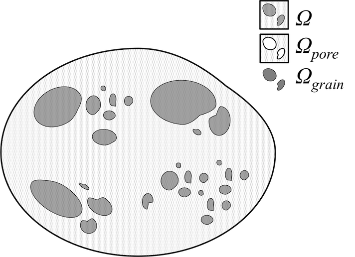
Figure 1: An illustration of a domain $\Omega$ consisting of a pore domain $\Omega_{\textrm{pore}}$, and a grain domain $\Omega_{\textrm{grain}}$.

2 Problem Formulation

We define $\Omega$, a two-dimensional domain consisting of a grain domain $\Omega_{\textrm{grain}}$, and a pore domain $\Omega_{\textrm{pore}}$ perforated by grains, see figure 1. Then, let $\varepsilon$ denote the diameter of the smallest grain. The steady-state Oseen’s problem is to find velocity $\vec{u}$ which is the solution to:

$$\mu\nabla^{2}\vec{u}+\rho(\vec{U}\cdot\nabla\vec{u})-\nabla p=\vec{f} \Omega_{\textrm{pore}}$$ in (1)

$$\nabla\cdot\vec{u}=0 \Omega_{\textrm{pore}}$$ in

where $\mu$ is the dynamic viscosity, $\rho$ is the density and $\vec{U}$ is a known velocity field.

The boundary condition of equation (1) is given by:

$$\vec{u} = \vec{g}\textrm{, on }\partial\Omega\cap\partial\Omega_{\textrm{pore}},$$ (2)

$$\vec{u} = \vec{U}\textrm{, when }\{x,y\}\rightarrow\infty,$$

where $\vec{f}$ is a source function, and $\vec{g}$ is a function fixed at the boundary $\partial\Omega$. In this paper, we consider only a no-slip condition on the grain boundaries: $\vec{u}\textrm{ at }{\partial\Omega_{\textrm{grain}}}=0$.

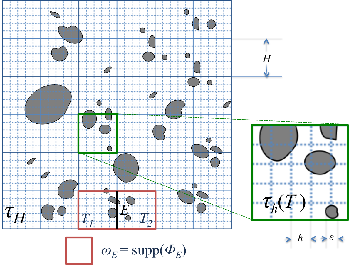
Figure 2: An illustration of the discretised domain $\tau_{H}$, and $\omega_{E}$ which is the support space for $\vec{\Phi}_{E}$.

3 Application of Crouzeix-Raviart MsFE

Here we explain the application of our method starting from the definition of the coarse and fine meshes. We then introduce the functional spaces for our multiscale basis functions and describe the construction of these functions within each coarse elements.

3.1 Discretisation

We discretise $\Omega$ into a two-dimensional homogeneous Cartesian coarse mesh $\mathcal{T}_{H}$ (see figure 2). $\mathcal{T}_{H}$ consists of coarse elements $T_{k},k=1,2,\dots,{N_{H}}$, where $N_{H}$ is the total number of coarse elements, each with width $H$. We define $\mathcal{E}_{H}$ the set of all coarse edges $E_{j},j=1,2,\dots,{N_{E}}$ in $\mathcal{T}_{H}$ including the edges on the domain boundary $\partial\Omega$. For each element $T$ we construct a fine mesh $\mathcal{T}_{h}(T)$, consisting of fine elements each with width $h$. Note that the combination of $\mathcal{T}_{h}(T)$ for all $T\in\mathcal{T}_{H}$ constructs a global fine mesh $\mathcal{T}_{h}$ which overlaps with $\mathcal{T}_{H}$. Conversely, one can generate $\mathcal{T}_{H}$ from $\mathcal{T}_{h}$ since the difference between the two meshes is only in the indexing.

3.2 Crouzeix–Raviart functional spaces

The functional spaces for velocity $V_{H}$, and for pressure $M_{H}$ are given below:

$$M_{H} = \{{q}\in L^{2}\,\mbox{such that}\,q=\mbox{constant, }\forall T\in\mathcal{T}_{H}\},$$ (3)

$$V_{H} = \{\vec{v}:\Omega\rightarrow R^{2}\,:\,\forall T\in\mathcal{T}_{H}\,\mbox{such that}$$

$$\mu\nabla^{2}\vec{v}+\rho(\vec{U}\cdot\nabla\vec{v})-\nabla s=0\textrm{, in }\Omega_{\textrm{pore}}\cap T$$

$$\nabla\cdot\,\vec{v}=\textrm{ constant in }\Omega_{\textrm{pore}}\cap T$$

$$\nabla\vec{v}\,n-sn=\textrm{ constant on }E\cap\Omega_{\textrm{pore}},\ \forall E\in\mathcal{E}(T)\}.$$

The key here is to maintain the continuity of (only) the average of $\vec{v}$ across an edge $E$: $\int_{E}[[\vec{v}]]=0$, where $[[{v}]]$ is the jump of the value $v$ across $E$. We wish to retain the advantage of our approach which has been successfully applied on Advection-Diffusion, and Stokes problems, namely: the weak imposing of continuity across element boundaries allows adaptive boundary conditions which relaxes the sensitivity of our method to random arrangements of grains, without the need of applying the more cumbersome oversampling methods.

3.3 Coarse-scale solution

By discretising $p$ into $p_{H}$ and $\vec{u}$ into $\vec{u}_{H}$, we can solve equation (1) in $\tau_{H}$ and rewrite it in a weak form as:

$$a(\vec{u}_{H},\vec{v}_{H})+c(\vec{u}_{H},\vec{v}_{H})+b(\vec{v}_{H},p_{H})= (\vec{v}_{H},\vec{f}) ,\forall\vec{v}_{H}\in V_{H}$$ (4)

$$b(\vec{u}_{H},q_{H})= 0 ,\forall q_{H}\in M_{H}$$

where

$$a(\vec{u},\vec{v}) = \int_{\Omega_{\textrm{pore}}}\mu\nabla\vec{u}:\nabla\vec{v}\hskip 8.53581ptd{\Omega_{\textrm{pore}}}$$ (5)

$$c(\vec{u},\vec{v})=c(\vec{U};\vec{u},\vec{v}) = \int_{\Omega_{\textrm{pore}}}\rho(\vec{U}\cdot\nabla\vec{u})\cdot\vec{v}\hskip 8.53581ptd{\Omega_{\textrm{pore}}}$$ (6)

$$b(\vec{v},q) = -\int_{\Omega_{\textrm{pore}}}q\nabla\cdot\vec{v}\hskip 8.53581ptd{\Omega_{\textrm{pore}}}.$$ (7)

The solution to problem (1) can then be approximated as linear combination of multiscale basis functions $\vec{\Phi}_{E,j}={\Phi}_{E}\vec{e}_{j}$, $j=1,2$ with $\{\vec{e}_{1},\vec{e}_{2}\}$ being the canonical basis of $\mathcal{R}^{2}$, such that:

$$\vec{u}_{H}(x,y)=\sum_{E\in\mathcal{E}(H),\,j=1,2}{u}_{E,j}\vec{\Phi}_{E,j}(x,y).$$ (8)

Consistent with the theory of MsFE method, the basis functions $\vec{\Phi}_{E,j}$ are themselves computed in the fine mesh constructed in each coarse elements.

3.4 Construction of a Crouzeix-Raviart basis

For each edge $E\in\mathcal{E}_{H}$ we construct $\vec{\Phi}_{E,i}\in V_{H}$, such that $\int_{E}\vec{\Phi}_{E,i}=\vec{e}_{i}$, and $\int_{E^{\prime}}\vec{\Phi}_{E,i}=0$ for all $E^{\prime}\in\mathcal{E}_{H}$, $E^{\prime}\not=E$. These functions form a basis of $V_{H}$, i.e

$$V_{H}=\textrm{span}\{\vec{\Phi}_{E,i},~{}E\in\mathcal{E}_{H},~{}i=1,2\}.$$ (9)

We also define $\textrm{supp}(\vec{\Phi}_{E,i})\subset\omega_{E}$, the ensemble of two quadrangles in $\mathcal{T}_{H}$ which share an edge $E$. Hence we solve for each coarse element $T_{k}$, a total of eight basis functions $\vec{\Phi}_{E,i}$ (and consequentially $\pi_{E,i}$) which are the solutions to:

$$\mu\nabla^{2}\vec{\Phi}_{E,i}+\rho(\vec{U}\cdot\nabla\vec{\Phi}_{E,i})-\nabla\pi_{E,i} = 0,\textrm{ in }\Omega_{\textrm{pore}}\cap T_{k},$$ (10)

$$\nabla\cdot\vec{\Phi}_{E,i} = \textrm{constant, in }\Omega_{\textrm{pore}}\cap T_{k},$$

$$\vec{\Phi}_{E,i} = 0,\textrm{ in }\Omega_{\textrm{grain}}\cap T_{k},$$

$$\nabla\vec{\Phi}_{E,i}n-\pi_{E,i}n = \textrm{constant, on }F\cap\Omega_{\textrm{pore}},\forall F\in\mathcal{E}(T_{k}),$$

$$\int_{F}\vec{\Phi}_{E,i} = \left\{\begin{array}[]{c}\vec{e}_{i},~{}F=E\\ 0,~{}F\not=E\end{array}\right.,\forall F\in\mathcal{E}(T_{k}),$$ (12)

$$\int_{\Omega_{\textrm{pore}}\cap T_{k}}\pi_{E,i} = 0.$$

To solve equation (10), we use Q1-Q1 finite element spaces in which both velocity and pressure degrees of freedom are defined on the same set of grid points. This arrangement is chosen due to the ease of programming and the computational efficiency. A stabilisation method is however necessary when this approach is considered. In a homogeneous Cartesian coordinate with fine element width of $h$, a stable solution can be achieved by perturbing the condition $\nabla\cdot\vec{\Phi}_{E,i}=0$ with a pressure Laplacian term (see Brezzi and Fortin (1991)). In a weak form, equation (10) reduces to finding $\vec{\Phi}_{E,i}\in H^{1}(T_{k}\cap\Omega_{\textrm{pore}})$, $\pi_{E,i}\in L^{2}_{0}(T_{k}\cap\Omega_{\textrm{pore}})$, and the Lagrange multipliers $\vec{\lambda}_{F}$, $\forall F\in\mathcal{E}(T_{k})$, where $\mathcal{E}(T_{k})$ is the set of all the edges of the quadrangle $T_{k}$, satisfying

$$\int_{T_{k}}\mu\nabla\vec{\Phi}_{E,i}:\nabla\vec{v}_{h}+\int_{T_{k}}\rho(\vec{U}\cdot\vec{\Phi}_{E,i})\cdot\vec{v}_{h}-\int_{T_{k}}\pi_{E,i}\nabla\cdot\vec{v}_{h}$$ (13)

$$+\sum_{F\in\mathcal{E}(T_{k})}\vec{\lambda}_{F}\cdot\int_{F}\vec{\Phi}_{E,i}=0,$$

$$-\int_{\Omega}q_{h}\nabla\cdot\vec{\Phi}_{E,i}-\theta h^{2}\int_{\Omega}\nabla\pi_{E,i}\cdot\nabla q_{h}=0,$$

$$\sum_{F\in\mathcal{E}(T_{k})}\vec{\mu}_{F}\cdot\int_{F}\vec{\Phi}_{E,i}=\vec{\mu}_{E}\cdot\vec{e}_{i},\quad\forall\vec{\mu}_{F}\in\textrm{R}^{2},~{}F\in\mathcal{E}(T_{k}).$$

Here, $\vec{v}_{h}$ and $q_{h}$ occupy the same finite element spaces as $\vec{\Phi}_{E,i}$ and $\pi_{E,i}$ respectively. $\theta$ is the stabilisation parameter which we set as $0.01$ for all our simulations (see Brezzi and Pitkäranta (1984)).

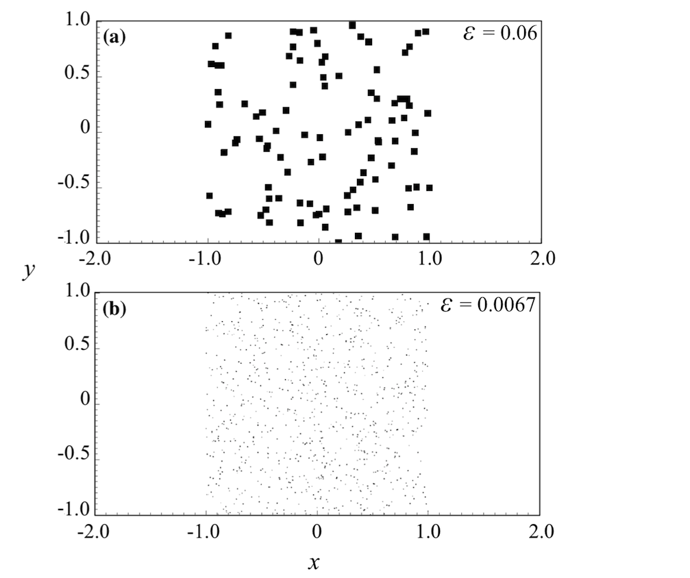
Figure 3: Two grain patterns in a channel consisting of randomly laid (a) 100 rectangular grains with width $\varepsilon=0.06$; and (b) 900 rectangular grains with $\varepsilon=0.0067$.

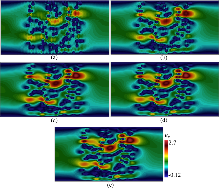
Figure 4: Contours of $u_{x}$ in a domain depicted in figure 3(a), with $\vec{U}=(0.002,0)$ computed using Crouzeix-Raviart MsFEM on (a) $32\times 16$; (b) $64\times 32$; (c) $128\times 64$; (d) $256\times 128$ coarse elements; and (e) the reference solution.

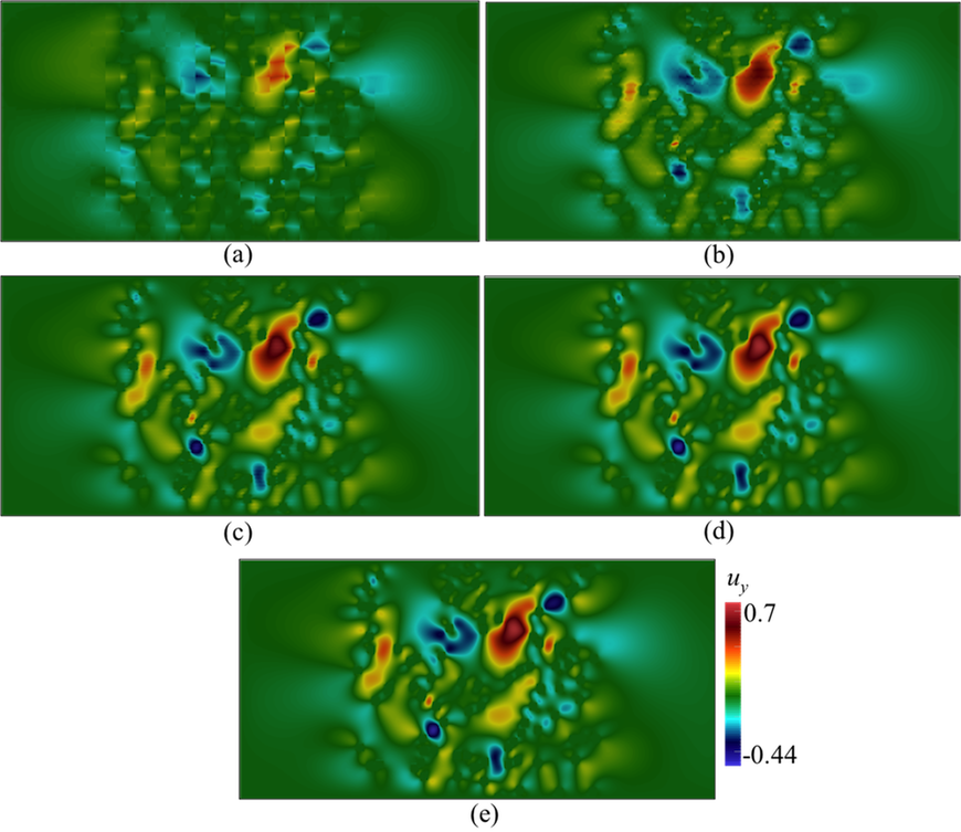
Figure 5: Contours of $u_{y}$ in a domain depicted in figure 3(a), with $\vec{U}=(0.002,0)$ computed using Crouzeix-Raviart MsFEM on (a) $32\times 16$; (b) $64\times 32$; (c) $128\times 64$; (d) $256\times 128$ coarse elements; and (e) the reference solution.

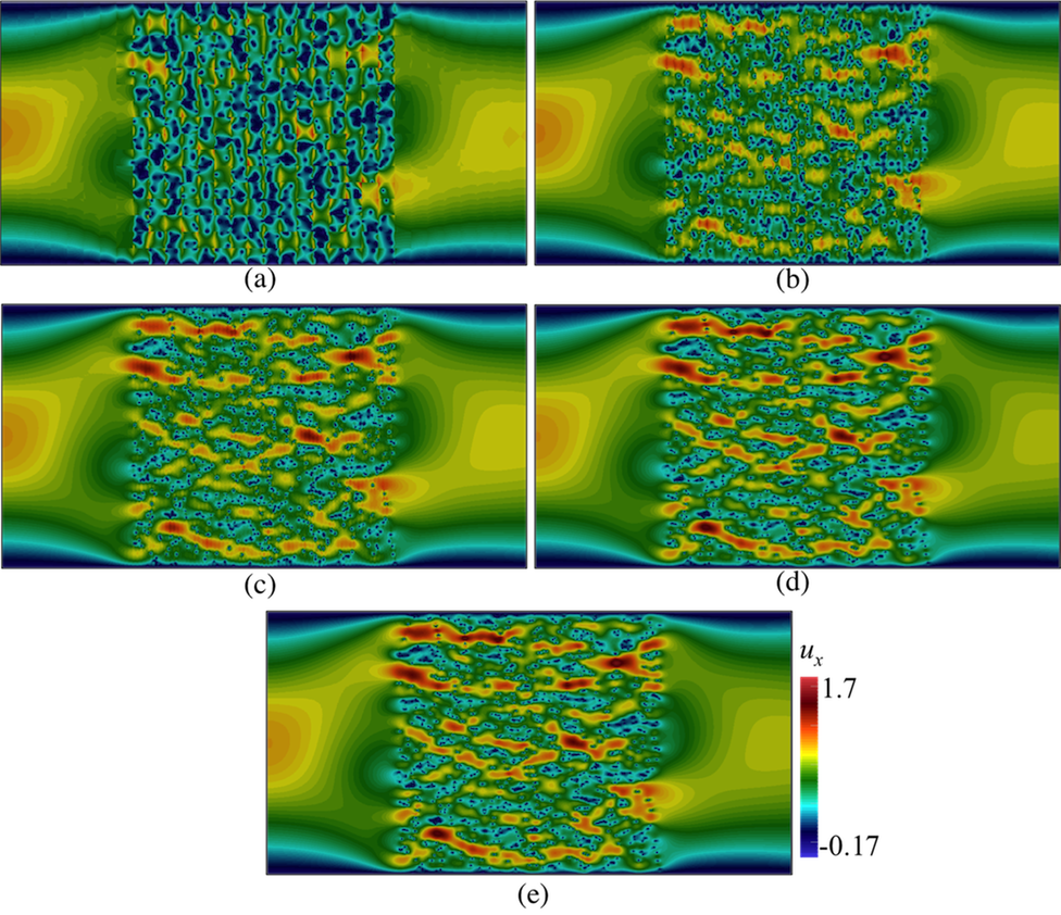
Figure 6: Contours of $u_{x}$ in a domain depicted in figure 3(b), with $\vec{U}=(0.002,0)$ computed using Crouzeix-Raviart MsFEM on (a) $32\times 16$; (b) $64\times 32$; (c) $128\times 64$; (d) $256\times 128$ coarse elements; and (e) the reference solution.

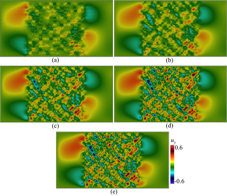
Figure 7: Contours of $u_{y}$ in a domain depicted in figure 3(b), with $\vec{U}=(0.002,0)$ computed using Crouzeix-Raviart MsFEM on (a) $32\times 16$; (b) $64\times 32$; (c) $128\times 64$; (d) $256\times 128$ coarse elements; and (e) the reference solution.

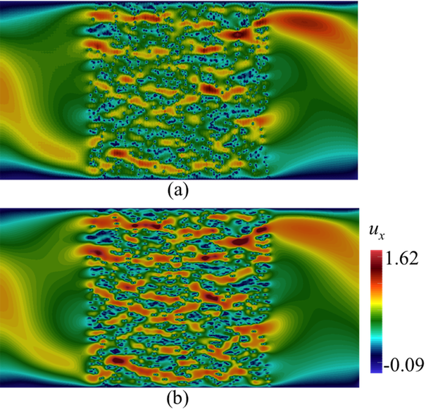
Figure 8: Contours of $u_{x}$ in a domain depicted in figure 3(b), with $\vec{U}$ according to equation (28), computed using Crouzeix-Raviart MsFEM on (a) $128\times 64$ coarse elements; compared with (b) the reference solution.

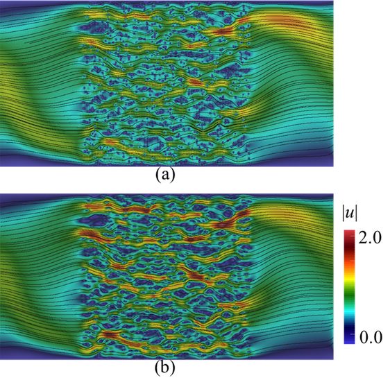
Figure 9: Contours of magnitude of velocity $|u|$ along with their streamlines in a domain depicted in figure 3(b), with $\vec{U}$ according to equation (28), computed using Crouzeix-Raviart MsFEM on (a) $128\times 64$ coarse elements; compared with (b) the reference solution.

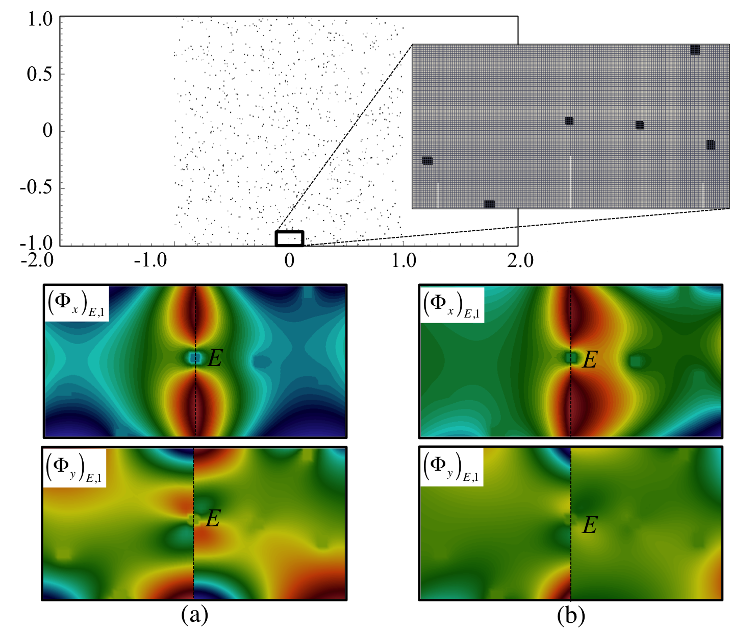
Figure 10: Multiscale basis functions $\vec{\Phi}_{E,j},j=1,2$ in the presence of grains of which, one coincides with the edge $E$. The basis functions depicted are for the given velocity field (a) $\vec{U}=0$; and (b) according to equation (28). In all cases, they successfully adapt to the worst-case scenario and maintain $\int_{E}\vec{\Phi}_{E,i}=\vec{e}_{1}$.

4 Penalization method

Often $\Omega_{\textrm{pore}}$ is a complicated pore structure in which solving equation (1) may require a complicated boundary-fitted, or even an unstructured mesh. In order to confine our computations in a homogeneous Cartesian mesh, we employ the penalization method Angot et al (1999). Henceforth, instead of solving equation (1) directly in $\Omega_{\textrm{pore}}$, we solve:

$$\mu_{\kappa}\nabla^{2}\vec{u}+\rho_{\kappa}(\vec{U}\cdot\nabla\vec{u})+\sigma_{\kappa}\vec{u}-\nabla p = \vec{f}_{\kappa}\textrm{, in }\Omega$$ (14)

$$\nabla\cdot\vec{u} = 0\textrm{, in }\Omega$$

$$\vec{u} = \vec{g}\textrm{, on }\partial\Omega$$

in which

$$\mu_{\kappa};\rho_{\kappa}=\left\{\begin{array}[]{cc}\frac{1}{h}&\mbox{ in $\Omega_{\textrm{grain}}$}\\ \mu;\rho&\mbox{ in $\Omega_{\textrm{pore}}$}\end{array}\right.,\sigma_{\kappa}=\left\{\begin{array}[]{cc}\frac{1}{h^{3}}&\mbox{ in $\Omega_{\textrm{grain}}$}\\ 0&\mbox{ in $\Omega_{\textrm{pore}}$}\end{array}\right.,\vec{f}_{\kappa}=\left\{\begin{array}[]{cc}0&\mbox{ in $\Omega_{\textrm{grain}}$}\\ \vec{f}&\mbox{ in $\Omega_{\textrm{pore}}$}\end{array}\right..$$ (21)

In our simulations the chosen fine-scale element width $h$ always satisfies $\varepsilon/h\geq 5$. The penalization coefficient $\sigma_{\kappa}$ then forces the solution $\vec{u}$ to vanish inside the obstacles. Other variants of penalization methods are studied in Angot et al (1999).

5 Reference solution

We use a Q1-Q1 finite element method to compute the reference solutions, as we do for computing $\vec{\Phi}$, in the global fine mesh $\mathcal{T}_{h}$. In a weak form, the solution to equation (1) are $\vec{u}_{h}$ and $p_{h}$ such that

$$\int_{\Omega}\mu_{\kappa}\nabla\vec{u}_{h}:\nabla\vec{v}_{h}+\int_{\Omega}\rho_{\kappa}(\vec{U}\cdot\nabla\vec{u}_{h})\cdot\vec{v}_{h}+\int_{\Omega}\sigma_{\kappa}\vec{u}_{h}\cdot\vec{v}_{h}$$ (22)

$$-\int_{\Omega}p_{h}\nabla\cdot\vec{v}_{h}=\int_{\Omega}\vec{v}_{h}\cdot\vec{f}_{\kappa},$$

$$-\int_{\Omega}q_{h}\nabla\cdot\vec{u}_{h}-\theta h^{2}(\nabla p_{h},\nabla q_{h})=0,$$

where $\vec{v}_{h}$, and $p_{h}$ occupy Q1-Q1 finite element spaces. We use the stabilization parameter $\theta=0.01$ throughout this paper Elman et al (2005). Note that other stable or stabilized elements can be used to provide the reference solution.

6 Boundary condition

Note that the boundary condition $\vec{u}=\vec{g}$ on $\partial\Omega$ is not included in equation (3). This is possible since we approximate the boundary condition in equation 10 only in a weak sense, i.e

$$\int_{E}\vec{u}_{H}=\int_{E}\vec{g},\quad\forall E\in\mathcal{E}_{H}\hskip 2.84526pt\textrm{on}\hskip 2.84526pt\partial\Omega.$$ (23)

Together with equation (8), we apply on the boundary $\partial\Omega$:

$$u_{E,i}=\int_{E}{\vec{g}\cdot\vec{e}_{i}}.$$ (24)

This approach has been applied successfully in Muljadi et al (2015b) for the Stokes equation, and is a modification with respect to previous work Bris et al (2013, 2014) where the boundary condition were strongly incorporated in the definition of $V_{H}$. Our approach therefore gives more flexibility when implementing non zero $\vec{g}$, i.e every basis functions $\vec{\Phi}_{E,i}$ including those on boundary $\partial\Omega$ can be computed in the same fashion—according to equation (10).

$N_{H}$	$L^{1}$ relative	$L^{2}$ relative	$H^{1}$ relative
$32\times 16$	0.13	0.142	0.222
$64\times 32$	0.08	0.088	0.172
$128\times 64$	0.052	0.060	0.089
$256\times 128$	0.012	0.013	0.07

Table 1: Convergence study of Poiseuille flow.

$N_{H}$	$(H/\varepsilon)$	$L^{1}$ relative	$L^{2}$ relative	$H^{1}$ relative
$32\times 16$	2.08	0.144	0.170	0.433
$64\times 32$	1.04	0.097	0.121	0.347
$128\times 64$	0.52	0.054	0.071	0.282
$256\times 128$	0.26	0.011	0.024	0.173

Table 2: Convergence study of channel flow pass pattern (a) with $\vec{U}=(0.002,0)$.

$N_{H}$	$(H/\varepsilon)$	$L^{1}$ relative	$L^{2}$ relative	$H^{1}$ relative
$32\times 16$	18.74	0.304	0.331	0.71
$64\times 32$	9.37	0.157	0.155	0.542
$128\times 64$	4.68	0.082	0.097	0.482
$256\times 128$	2.34	0.037	0.049	0.239

Table 3: Convergence study of channel flow pass pattern (b) with $\vec{U}=(0.002,0)$.

$N_{H}$	$(H/\varepsilon)$	$L^{1}$ relative	$L^{2}$ relative	$H^{1}$ relative
$32\times 16$	18.74	0.32	0.355	0.80
$64\times 32$	9.37	0.153	0.161	0.567
$128\times 64$	4.68	0.077	0.102	0.442
$256\times 128$	2.34	0.038	0.043	0.319

Table 4: Convergence study of channel flow pass pattern (b) with $\vec{U}$ according to equation (28).

7 Numerical Results

We consider a channel domain $\Omega=[-2\leq x\leq 2,-1\leq y\leq 1]$ containing a porous medium spanning from $x=-1$ to $x=1$. We then assign $\rho=1$, $\mu=0.001$, and $\vec{f}=0$. At the inlet, the theoretical incompressible Poiseuille solution (parabolic velocity profile) is applied for all cases, i.e $\vec{u}=\left(1-y^{2},0\right)$ on $x=-2$, whereas the Neumann boundary condition $\partial u/\partial n=0$ is assumed at the outlet, $x=2$. No–slip boundary conditions at the top and bottom walls are applied.

First we apply our method on simple Poiseuille flow without any porous bodies. Then two grain patterns are included, see figure 3. From here on we refer to them as pattern (a) depicted in figure 3(a), and pattern (b) depicted in figure 3(b). Pattern (a) consists of 100 randomly placed grains, each with width $\varepsilon=0.06$. Pattern (b) consists of 900 grains with $\varepsilon=0.0067$.

We compare all our results to the reference solutions. When computing the reference solutions, we employ Q1-Q1 finite element method on a fine mesh consisting of $2560\times 1280$ quadrangles. This ensures the ratio $\varepsilon/h\geq 5$.

7.1 Poiseuille flow

We apply a vector field $\vec{U}=\left(0.002,0\right)$ corresponding to $\textrm{Re}\approx 4$ where $\textrm{Re}=\frac{\rho\varepsilon|\vec{U}|}{\mu}$ (in the absence of grains, we assume that $\varepsilon$ is the channel diameter). In table 1, the norms of error of the Crouzeix-Raviart MsFEM solutions relative to the reference solution on a number of coarse meshes are given, showing a convincingly converging trend.

7.2 Pattern (a)

Here we test our method in solving flow pass a porous body with a random pattern of grains. We consider pattern (a) where each grain is a rectangle with width $\varepsilon=0.06$, $\textrm{Re}\approx 0.12$. In figures 4 and 5 the contours of velocity components $u_{x}$ and $u_{y}$ computed on a number coarse meshes are given. The results are compared to the reference solution. The contours computed using Crouzeix-Raviart MsFEM at $256\times 128$ are identical to the reference solution; however, even at $32\times 16$, the flow features already resemble those of the reference solution, and at $64\times 32$ without any appreciable difference. Norms of error relative to the reference solution in $L^{1},L^{2}$, and $H^{1}$ spaces are given in table 2 showing a converging behaviour.

7.3 Pattern (b)

Here we simulate flow pass pattern (b) which contains finer ($\varepsilon=0.0067$) and much more grains. We use the same kinds of coarse meshes, and vector field $\vec{U}$ as in the previous tests, which corresponds to $\textrm{Re}\approx 0.013$. This is a more challenging test than the previous ones due to much larger $H/\varepsilon$ ratios—ranging from $18.74$ to $2.34$. This means each coarse elements in the vicinity of the grains has higher chances of being occupied by more than one grain, and therefore suffers more oscillations.

In figures 6 and 7 the contours of $u_{x}$ and $u_{y}$ are given. As in the previous tests, the results are compared to the reference solution. The contours of ${u}_{x}$ and $u_{y}$ computed using Crouzeix-Raviart MsFEM at $256\times 128$ are obviously identical to those of the reference solution. The results at $64\times 32$ however already exhibit similar main flow features to the reference solution. This shows that the multiscale basis functions do well in capturing highly oscillatory fine-scale solutions. Similarly monotonically decreasing relative error norms are shown in table 3.

7.4 Heterogeneous velocity field $\vec{U}$

To further test the feasibility of our method, we apply a heterogeneous velocity field

$$\vec{U}=\left(\begin{array}[]{rl}\begin{array}[]{cc}2y(1-0.25x^{2})\\ -x(1-y^{2})\end{array}\end{array}\right)\textrm{ , in }\Omega_{\textrm{pore}}.$$ (28)

In figures 8 the contours of $u_{x}$ through pattern (b) computed using Crouzeix-Raviart MsFEM on $128\times 64$ coarse elements; and the reference solution are compared. The flow features are noticeably different than the previous results especially in regions away from the porous body. Indeed at the farthest from grains, the flow experiences $\textrm{Re}\approx 80$ where the inertial effect manifests the most. In table 4, the convergence study is given for a range of coarse meshes. Again we can see that our method gives good qualitative and quantitative agreement with the reference solution. In figures 9 the contours of the magnitude of velocity computed using Crouzeix-Raviart MsFEM on $128\times 64$ coarse elements are displayed along with their streamlines and compared with the reference solution. We notice that the Crouzeix-Raviart MsFEM gives an excellent agreement in terms of flow pattern with the reference solution.

In figures 10, we plot the multiscale basis function $\vec{\Phi}$ associated to the highlighted patch in the computational domain with pattern (b). We select this patch to illustrate the behaviour of $\vec{\Phi}$ at a worst-case scenario: a grain coinciding with a coarse element edge $E$. Figure 10(a) shows the basis functions $\vec{\Phi}_{E,1}$ computed with $\vec{U}=0$, the Oseen problem therefore reduces to a Stokes problem. Figure 10(b) shows the basis functions $\vec{\Phi}_{E,1}$ computed with $\vec{U}$ according to equation (28). We notice the difference in the behaviour of $\vec{\Phi}$ due to different $\vec{U}$. In any cases the basis functions succesfully adapt to the presence of a grain at the edge $E$ and maintain $\int_{E}\vec{\Phi}_{E,i}=\vec{e}_{i}$.

8 Concluding remarks

The Crouzeix-Raviart MsFEM has been developed and tested for solving Oseen’s approximation for incompressible flow around solid bodies. The method performs very well in the presence of non-periodic grain formations. The weakly enforced continuity across coarse element edges ensures accurate basis function solutions without any oversampling methods. The basis functions are shown to successfully capture the effects of homogeneous and inhomogeneous vector field $\vec{U}$. The penalization method is seamlessly incorporated into our method allowing an extensive utilisation of simple Cartesian mesh.

This method is developed as a stepping stone towards solving then more complicated Navier-Stokes equation. Although only two-dimensional cases are considered, the extension of this work on three-dimensions is straightforward. Similarly the method can be applied for inhomogeneous Oseen’s problem with $\vec{f}\neq 0$. The reconstruction of fine-scale pressure is not the focus of the current work although it is possible (see Muljadi et al (2015b)). The calculations of MsFEM basis functions within a coarse element are done independent of the neighbouring elements which makes it suitable for the application of parallel programming.

For practical applications, the method is a promising development towards simulations capable of handling a wide range of spatial scales, while accommodating non-linear effects.

9 Acknowledgement

I thank the Engineering and Physical Science Research Council for financial support through grant number EP/L012227/1. I also thank Prof. Martin Blunt, and Prof. Pierre Degond for their invaluable advises. The source codes for the simulations in this paper are available at https://www.imperial.ac.uk/engineering/departments/earth-science/research/research-groups/perm/research/pore-scale-modelling/software/

References

- Aarnes et al (2005) Aarnes JE, Kippe V, Lie KA (2005) Mixed multiscale finite elements and streamline methods for reservoir simulation of large geomodels. Advances in Water Resources 28(3):257 – 271, DOI http://dx.doi.org/10.1016/j.advwatres.2004.10.007, URL http://www.sciencedirect.com/science/article/pii/S0309170804001885
- Angot et al (1999) Angot P, Bruneau CH, Fabrie P (1999) A penalization method to take into account obstacles in incompressible viscous flows. Numerische Mathematik 81(4):497–520, DOI 10.1007/s002110050401, URL http://dx.doi.org/10.1007/s002110050401
- Blunt et al (2013) Blunt MJ, Bijeljic B, Dong H, Gharbi O, Iglauer S, Mostaghimi P, Paluszny A, Pentland C (2013) Pore-scale imaging and modelling. Advances in Water Resources 51:197–216, DOI 10.1016/j.advwatres.2012.03.003, URL 10.1016/j.advwatres.2012.03.003
- Brezzi and Fortin (1991) Brezzi F, Fortin M (1991) Mixed and Hybrid Finite Element Methods. Springer-Verlag New York, Inc., New York, NY, USA
- Brezzi and Pitkäranta (1984) Brezzi F, Pitkäranta J (1984) Efficient Solutions of Elliptic Systems: Proceedings of a GAMM-Seminar Kiel, January 27 to 29, 1984. Vieweg+Teubner Verlag, Wiesbaden, DOI 10.1007/978-3-663-14169-3˙2, URL http://dx.doi.org/10.1007/978-3-663-14169-3_2
- Bris et al (2013) Bris C, Legoll F, Lozinski A (2013) MsFEM à la crouzeix-raviart for highly oscillatory elliptic problems. Chinese Annals of Mathematics, Series B 34(1):113–138, DOI 10.1007/s11401-012-0755-7, URL http://dx.doi.org/10.1007/s11401-012-0755-7
- Bris et al (2014) Bris CL, Legoll F, Lozinski A (2014) An msfem type approach for perforated domains. Multiscale Modeling & Simulation 12(3):1046–1077, DOI 10.1137/130927826, URL http://dx.doi.org/10.1137/130927826
- Chu et al (2008) Chu J, Efendiev Y, Ginting V, Hou T (2008) Flow based oversampling technique for multiscale finite element methods. Advances in Water Resources 31(4):599 – 608, DOI http://dx.doi.org/10.1016/j.advwatres.2007.11.005, URL http://www.sciencedirect.com/science/article/pii/S030917080700173X
- Chung et al (0) Chung ET, Efendiev Y, Li G, Vasilyeva M (0) Generalized multiscale finite element methods for problems in perforated heterogeneous domains. Applicable Analysis 0(0):1–26, DOI 10.1080/00036811.2015.1040988, URL http://dx.doi.org/10.1080/00036811.2015.1040988
- Crouzeix and Raviart (1973) Crouzeix M, Raviart PA (1973) Conforming and nonconforming finite element methods for solving the stationary stokes equations i. ESAIM: Mathematical Modelling and Numerical Analysis - Modélisation Mathématique et Analyse Numérique 7(R3):33–75, URL http://eudml.org/doc/193250
- Degond et al (2015) Degond P, Lozinski A, Muljadi BP, Narski J (2015) Crouzeix-raviart MsFEM with bubble functions for diffusion and advection-diffusion in perforated media. Communications in Computational Physics 17:887–907, DOI 10.4208/cicp.2014.m299, URL http://journals.cambridge.org/article_S1815240615000237
- Efendiev et al (2013) Efendiev Y, Galvis J, Hou TY (2013) Generalized multiscale finite element methods (gmsfem). J Comput Phys 251:116–135, DOI 10.1016/j.jcp.2013.04.045, URL http://dx.doi.org/10.1016/j.jcp.2013.04.045
- Elman et al (2005) Elman H, Silvester DJ, Wathen AJ (2005) Finite Elements and Fast Iterative Solvers : with Applications in Incompressible Fluid Dynamics. Oxford University Press
- Henning and Peterseim (2013) Henning P, Peterseim D (2013) Oversampling for the multiscale finite element method. Multiscale Modeling & Simulation 11(4):1149–1175, DOI 10.1137/120900332, URL http://dx.doi.org/10.1137/120900332
- Hou and Wu (1997) Hou TY, Wu XH (1997) A multiscale finite element method for elliptic problems in composite materials and porous media. Journal of Computational Physics 134(1):169 – 189, DOI http://dx.doi.org/10.1006/jcph.1997.5682, URL http://www.sciencedirect.com/science/article/pii/S0021999197956825
- Jenny et al (2003) Jenny P, Lee S, Tchelepi H (2003) Multi-scale finite-volume method for elliptic problems in subsurface flow simulation. Journal of Computational Physics 187(1):47 – 67, DOI http://dx.doi.org/10.1016/S0021-9991(03)00075-5, URL http://www.sciencedirect.com/science/article/pii/S0021999103000755
- Lipnikov et al (2011) Lipnikov K, Moulton JD, Svyatskiy D (2011) Adaptive strategies in the multilevel multiscale mimetic method for two-phase flows in porous media. Multiscale Modeling & Simulation 9(3):991–1016, DOI 10.1137/100787544, URL http://dx.doi.org/10.1137/100787544
- Mostaghimi et al (2012) Mostaghimi P, Blunt MJ, Bijeljic B (2012) Computations of absolute permeability on micro-ct images. Mathematical Geosciences 45(1):103–125, DOI 10.1007/s11004-012-9431-4, URL http://dx.doi.org/10.1007/s11004-012-9431-4
- Muljadi et al (2015a) Muljadi BP, Blunt MJ, Raeini AQ, Bijeljic B (2015a) The impact of porous media heterogeneity on non-darcy flow behaviour from pore-scale simulation. Advances in Water Resources pp –, DOI http://dx.doi.org/10.1016/j.advwatres.2015.05.019
- Muljadi et al (2015b) Muljadi BP, Narski J, Lozinski A, Degond P (2015b) Nonconforming multiscale finite element method for stokes flows in heterogeneous media. part i: Methodologies and numerical experiments. Multiscale Modeling & Simulation 13(4):1146–1172, DOI 10.1137/14096428X, URL http://dx.doi.org/10.1137/14096428X
- Scheibe et al (2015) Scheibe TD, Murphy EM, Chen X, Rice AK, Carroll KC, Palmer BJ, Tartakovsky AM, Battiato I, Wood BD (2015) An analysis platform for multiscale hydrogeologic modeling with emphasis on hybrid multiscale methods. Groundwater 53(1):38–56, DOI 10.1111/gwat.12179, URL http://dx.doi.org/10.1111/gwat.12179
- Wesseling (1992) Wesseling P (1992) An introduction to multigrid methods. Pure and applied mathematics, John Wiley & Sons Australia, Limited, URL https://books.google.co.uk/books?id=MznvAAAAMAAJ