Tangled up in Blue
A Survey on Connectivity, Decompositions, and Tangles

Abstract

We survey an abstract theory of connectivity, based on symmetric submodular set functions. We start by developing Robertson and Seymour’s [44] fundamental duality theory between branch decompositions (related to the better-known tree decompositions) and so-called tangles, which may be viewed as highly connected regions in a connectivity system. We move on to studying canonical decompositions of connectivity systems into their maximal tangles. Last, but not least, we will discuss algorithmic aspect of the theory.

1 Introduction

Suppose we have some structure, maybe a graph, a hypergraph, or maybe something entirely different like a set of vectors in Euclidean space. Let ${U}$ be the universe of our structure. We want to study partitions, or separations, as we prefer to call them, of ${U}$ (see Figure 1.1). A connectivity function assigns to each separation a nonnegative integer, which we call the order of the separation. For example, ${U}$ may be the vertex set of a graph and the order of a separation (or cut) $(X,\overline{X})$ could be the number of edges from $X$ to $\overline{X}$. This is what is known as “edge connectivity” in a graph. Or ${U}$ could be the edge set of a graph, and the order of a separation $(X,\overline{X})$ the number of vertices incident with an edge in $X$ and an edge in $\overline{X}$. We will give precise definitions as well as many more examples in Section 2.

Figure 1.1: A separation $(X,\overline{X})$ of ${U}$

The guiding questions in this survey are the following.

Question 1:

How can we decompose a connectivity system along low order separations?

Question 2:

What are the highly connected regions of a connectivity system?

Obviously, the two questions are complementary: highly connected regions should be precisely those regions that have no low order separations. We will see that there is a precise technical duality that captures this intuition (the Duality Theorem 6.1).

While it is relatively straightforward to give a satisfactory definition of decomposition—branch decomposition (see Section 3)—it is less obvious what a “highly connected region” is supposed to be. The fact that we use the unspecific term “region” instead of something specific such as “$k$-connected component” already indicates this. Indeed, it is an old and well-known problem in graph theory, going back to Tutte, to find decompositions of graphs into $k$-connected components, for any $k\geq 4$. Satisfactory decompositions of graphs into $k$-connected components only exist for $k\leq 3$. Even for $k=3$ the decomposition is starting to get elusive, because the 3-connected components of a graph are not subgraphs: they may contain so-called “virtual edges” that are not present in the graph. The problem (and also a solution to this problem) can be illustrated on a hexagonal grid (see Figure 1.2). To avoid irregularities at the boundary, it is best to think of the grid as being embedded on a torus. Clearly, such a grid is not $4$-connected: the three neighbours of any vertex form a vertex-separator of order $3$ (see Figure 1.3(a)). But there is no obvious notion of “4-connected component” of such a grid, because the separations of order $4$ may overlap (see Figure 1.3(b)).

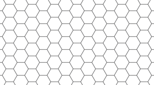
Figure 1.2: A hexagonal grid

Figure 1.3: Separations of a hexagonal grid

Observe, however, that in every separation of order $3$ of the grid, one side of separation only consists of a single vertex. If we ignore separations that are so extremely unbalanced and only look at separations where both sides have, say, a constant fraction of the vertices, then the grid suddenly becomes highly connected: if the grid is square then the smallest balanced separation has order square root of the number of vertices. This is a well-studied notion of “high connectivity”. For example, expander graphs are highly connected in this sense. It is also the notion of “high connectivity” we will be interested in here. It will lead us to well-linked sets (see Section 4) and ultimately tangles (see Section 5), which describe the highly connected regions in a connectivity system.

After establishing the basic duality between decompositions and tangles (see Section 6), we shall prove that every connectivity system has a canonical decomposition into its maximal tangles, which may be viewed as an analogue of the decomposition into $k$-connected components for $k>3$ (see Section 7) .

The final Section 8 is devoted to algorithmic aspects of the theory.

The goal of this survey is to lay out the basic theory sketched above. It is not my intention (and beyond my abilities) to comprehensively cover all results on connectivity functions, decompositions, and tangles.

2 Connectivity Functions

We start by discussing a few basic properties of set functions. Let ${U}$ be a finite set, our universe. Whenever the universe ${U}$ is clear from the context (which it will be most of the time), we denote the complement ${U}\setminus X$ of a set $X\subseteq{U}$ by $\overline{X}$. Let $\varphi:2^{U}\to{\mathbb{Z}}$ be an integer-valued function defined on the subsets of ${U}$.

• $\varphi$ is symmetric if $\varphi(X)=\varphi(\overline{X})$ for all $X\subseteq{U}$.

• $\varphi$ is monotone if $\varphi(X)\subseteq\varphi(Y)$ for all $X\subseteq Y\subseteq{U}$.

• $\varphi$ is submodular if

  $$\varphi(X)+\varphi(Y)\geq\varphi(X\cap Y)+\varphi(X\cup Y)$$ (2.)

  for all $X,Y\subseteq{U}$.

• $\varphi$ is posimodular if

  $$\varphi(X)+\varphi(Y)\geq\varphi(X\setminus Y)+\varphi(Y\setminus X)$$ (2.)

  for all $X,Y\subseteq{U}$.

• $\varphi$ is normalised if $\varphi(0)=0$.

• $\varphi$ is nontrivial if $\varphi(X)\neq 0$ for some $X\subseteq{U}$.

Note that for every integer $c$ the function $\varphi-c:X\mapsto\varphi(X)-c$ is symmetric, monotone, submodular, posimodular, respectively, if and only if $\varphi$ is. In particular, this is the case for the normalised function $\varphi_{0}:=\varphi-\varphi(\emptyset)$. For this reason, we can usually assume, without loss of generality, that our set functions are normalised. The valence of $\varphi$ is

$$\operatorname{val}(\varphi):=\max\{|\varphi(\{u\})-\varphi(0)|\mid u\in{U}\}$$

if ${U}\neq\emptyset$ and $\operatorname{val}(\varphi):=0$ if ${U}=\emptyset$. Of course if $\varphi$ is normalised and ${U}$ is nonempty, $\operatorname{val}(\varphi)$ is just the maximum of the singleton values of $\varphi$. We call $\varphi$ univalent if $\operatorname{val}(\varphi)=1$.

Definition 2.1.

A connectivity function on ${U}$ is a normalised, symmetric, and submodular set function $\kappa:2^{U}\to{\mathbb{Z}}$.

If $\kappa$ is a connectivity function on ${U}$, we call the pair $({U},\kappa)$ a connectivity system. Before we give examples, we collect a few basic properties of connectivity functions in the following lemma.

Lemma 2.2.

Let $\kappa$ be a connectivity function on ${U}$.

1. $\kappa$ is posimodular.

2. $\kappa$ is nonnegative, that is, $\kappa(X)\geq 0$ for all $X\subseteq{U}$.

3. $|\kappa(X)-\kappa(Y)|\leq\sum_{x\in X\triangle Y}\kappa(x)\leq\operatorname{val}(\kappa)\cdot|X\triangle Y|$, for all $X,Y\subseteq{U}$.

By $X\triangle Y$ we denote the symmetric difference of $X$ and $Y$.

Proof of Lemma 2.2.

To prove (1), let $X,Y\subseteq{U}$. Then

$$\kappa(X)+\kappa(Y) =\kappa(X)+\kappa(\overline{Y})$$ by symmetry

$$\geq\kappa(X\cap\overline{Y})+\kappa(X\cup\overline{Y})$$ by submodularity

$$\geq\kappa(X\cap\overline{Y})+\kappa(\overline{X}\cap Y)$$ by symmetry

$$=\kappa(X\setminus Y)+\kappa(Y\setminus X).$$

To prove (2), let $X\subseteq{U}$. Then

$$2\cdot\kappa(X)=\kappa(X)+\kappa(\overline{X})\geq\kappa(\emptyset)+\kappa({U})=2\cdot\kappa(\emptyset)=0.$$

To prove (3), it clearly suffices to prove that for every $X\subseteq{U}$ and $x\in{U}\setminus X$ we have

$$\kappa(X)-\kappa(\{x\})\leq\kappa(X\cup\{x\})\leq\kappa(X)+\kappa(\{x\}).$$

Indeed,

$$\kappa(X)+\kappa(\{x\})\geq\kappa(\emptyset)+\kappa(X\cup\{x\})=\kappa(X\cup\{x\}),$$

which implies the second inequality, and

$$\kappa(X\cup\{x\})+\kappa(\{x\})=\kappa(X\cup\{x\})+\kappa(\overline{\{x\}})\geq\kappa(X)+\kappa({U})=\kappa(X),$$

which implies the first inequality. ∎

Corollary 2.3.

A connectivity function $\kappa$ is nontrivial if and only if $\operatorname{val}(\kappa)\geq 1$.

It may also be worth noting that the trivial function $X\mapsto 0$ is the only connectivity function on a set ${U}$ of cardinality $|{U}|\leq 1$. We denote the trivial connectivity function on the empty set by $\kappa_{\emptyset}$.

Let $\kappa$ be a connectivity function on a set ${U}$, and let $X,Y\subseteq{U}$ be disjoint. An $(X,Y)$-separation is a set $Z$ such that $X\subseteq Z\subseteq\overline{Y}$. Observe that if $Z$ is an $(X,Y)$-separation then $\overline{Z}$ is a $(Y,X)$-separation. An $(X,Y)$-separation $Z$ is minimum if its order $\kappa(Z)$ is minimal.

The following lemma gives a first indication of the value of submodularity in this context.

Lemma 2.4.

Let $\kappa$ be a connectivity function on a set ${U}$, and let $X,Y\subseteq{U}$ be disjoint. Then there is a (unique) minimum $(X,Y)$-separation $Z$ such that $Z\subseteq Z^{\prime}$ for all minimum $(X,Y)$-separations $Z^{\prime}$.

We call $Z$ the leftmost minimum $(X,Y)$-separation.

Proof.

Let $Z$ be a minimum $(X,Y)$ separation of minimum cardinality $|Z|$, and let $Z^{\prime}$ be another minimum $(X,Y)$-separation. Then both $Z\cap Z^{\prime}$ and $Z\cup Z^{\prime}$ are $(X,Y)$-separations, and thus $\kappa(Z\cap Z^{\prime}),\kappa(Z\cup Z^{\prime})\geq\kappa(Z)=\kappa(Z^{\prime})$. By submodularity, this implies $\kappa(Z\cap Z^{\prime})=\kappa(Z\cup Z^{\prime})=\kappa(Z)=\kappa(Z^{\prime})$. By the minimality of $|Z|$, we have $|Z|\leq|Z\cap Z^{\prime}|$, and this implies $Z\subseteq Z^{\prime}$. ∎

2.1 Examples

Before we move on with the theory, we consider a number of examples of connectivity functions from different domains. We discuss these examples in great detail; in particular, we often give full (and tedious) proofs of submodularity. The reader should feel free to skip these proofs. To get a feeling for how these proofs go, I do recommend to look at the proof in Example 2.5, which is the simplest.

Our first two examples capture precisely what is known as edge-connectivity and vertex-connectivity in a graph.

Example 2.5 (Edge Connectivity).

Let $G$ be a graph. For all sets $X,Y\subseteq V(G)$ we let $E(X,Y)$ be the set of all edges with one endvertex in $X$ and one endvertex in $Y$. We define the edge-connectivity function $\nu_{G}$ on $V(G)$ by

$$\nu_{G}(X):=|E(X,\overline{X})|.$$

We claim that $\nu_{G}$ is a connectivity function. We obviously have $\nu_{G}(\emptyset)=0$. The function $\nu_{G}$ is symmetric, because $E(X,\overline{X})=E(\overline{X},X)$. To see that it is submodular, let $X,Y\subseteq V(G)$. We have

$$\nu_{G}(X)=\, |E(X\cap Y,\overline{X}\cap Y)|+|E(X\cap Y,\overline{X}\cap\overline{Y})|$$

$$+|E(X\cap\overline{Y},\overline{X}\cap Y)|+|E(X\cap\overline{Y},\overline{X}\cap\overline{Y})|,$$

$$\nu_{G}(Y)=\, |E(X\cap Y,X\cap\overline{Y})|+|E(X\cap Y,\overline{X}\cap\overline{Y})|$$

$$+|E(\overline{X}\cap Y,X\cap\overline{Y})|+|E(\overline{X}\cap Y,\overline{X}\cap\overline{Y})|,$$

$$\nu_{G}(X\cap Y)=\, |E(X\cap Y,\overline{X}\cap Y)|+|E(X\cap Y,\overline{X}\cap\overline{Y})|+|E(X\cap Y,X\cap\overline{Y})|,$$

$$\nu_{G}(X\cup Y)=\, |E(X\cap Y,\overline{X}\cap\overline{Y})|+|E(\overline{X}\cap Y,\overline{X}\cap\overline{Y})|+|E(X\cap\overline{Y},\overline{X}\cap\overline{Y})|$$

(see Figure 2.1). Comparing the sums of the first two and the last two equations yields the submodularity inequality

$$\nu_{G}(X)+\nu_{G}(Y)\geq\nu_{G}(X\cap Y)+\nu_{G}(X\cup Y).$$

Hence $\nu_{G}$ is a connectivity function. Note that $\operatorname{val}(\nu_{G})$ is the maximum degree of $G$. $\lrcorner$

Figure 2.1: Crossing separations

Example 2.6 (Vertex Connectivity, [42]).

Let $G$ be a graph. We define the boundary $\partial(X)$ of an edge set $X\subseteq E(G)$ to be the set of vertices incident with both an edge in $X$ and an edge in $E(G)\setminus X$. We define the vertex-connectivity function $\kappa_{G}$ on the edge set $E(G)$ by

$$\kappa_{G}(X):=|\partial(X)|.$$

for all $X\subseteq E(G)$.

We claim that $\kappa_{G}$ is a connectivity function. Obviously, $\kappa_{G}(\emptyset)=\emptyset$ and $\kappa_{G}$ is symmetric. To prove that it is submodular, let $X,Y\subseteq E(G)$. We need to prove

$$\kappa_{G}(X)+\kappa_{G}(Y)\geq\kappa_{G}(X\cap Y)+\kappa_{G}(X\cup Y).$$ (2.)

On the right-hand side of the inequality (2.),

1. all vertices incident with edges in both $X\cap Y$, $\overline{X}\cap\overline{Y}$ are counted twice, and

2. of the remaining vertices all vertices incident with edges in both $X\cap Y$, $\overline{X}\cap Y$ or both $X\cap Y$, $X\cap\overline{Y}$ are counted once in $\kappa_{G}(X\cap Y)$, and all vertices incident with edges in both $\overline{X}\cap Y$, $\overline{X}\cap\overline{Y}$ or both $X\cap\overline{Y}$, $\overline{X}\cap\overline{Y}$ are counted once in $\kappa_{G}(X\cup Y)$

(again, Figure 2.1 may be helpful).

On the left-hand side, the vertices in (i) are counted twice as well, and the vertices in (ii) are counted at least once, those incident with edges in both $X\cap Y$, $\overline{X}\cap Y$ and those incident with edges in both $X\cap\overline{Y}$, $\overline{X}\cap\overline{Y}$ in $\kappa_{G}(X)$ and those incident with edges in both $X\cap Y$, $X\cap\overline{Y}$ and those incident with edges in both $\overline{X}\cap Y$, $\overline{X}\cap\overline{Y}$ in $\kappa_{G}(Y)$. This proves the inequality.

Note that $\operatorname{val}(\kappa_{G})\leq 2$, where equality holds if and only if $G$ contains a triangle or a path of length $3$. $\lrcorner$

Example 2.7 (Hypergraph Connectivity).

We can easily generalise the edge-connectivity and vertex-connectivity functions from graphs to hypergraphs. Let $H$ be a hypergraph with vertex set $V(H)$ and edge set $E(H)\subseteq 2^{V(H)}$. We define the edge-connectivity function $\nu_{H}:2^{V(H)}\to{\mathbb{N}}$ by

$$\nu_{H}(X):=\big{|}\{e\in E(H)\;\big{|}\;e\cap X\neq\emptyset\text{ and }e\cap\overline{X}\neq\emptyset\}\big{|}$$

and the vertex-connectivity function $\kappa_{H}:2^{E(H)}\to{\mathbb{N}}$ by

$$\kappa_{H}(Y):=|\partial(Y)|=\big{|}\{v\in V(H)\;\big{|}\;\exists e\in Y,e^{\prime}\in\overline{Y}:\;v\in e\cap e^{\prime}\}\big{|}.$$

We leave it as an exercise to the reader to verify that these are indeed connectivity functions.

Note the duality between the two functions: if by $\widetilde{H}$ we denote the dual hypergraph with vertex set $E(H)$ and edges $e_{v}:=\{e\in E(H)\mid v\in e\}$ for all $v\in V$, which is actually a multi-hypergraph, we have $\nu_{\widetilde{H}}=\kappa_{H}$ and, identifying each vertex $v\in V(H)$ with the edge $e_{v}\in E(\widetilde{H})$, also $\kappa_{\widetilde{H}}=\nu_{H}$. $\lrcorner$

Example 2.8 (Matching Connectivity, [47] (also see [32])).

There is an alternative connectivity function capturing vertex connectivity in a graph $G$. As opposed to the function $\kappa_{G}$, it is defined on the vertex set of $G$. For disjoint subsets $X,Y\subseteq V(G)$, an $(X,Y)$-matching is a set $M\subseteq E(G)$ of mutually disjoint edges that all have an endvertex in $X$ and an endvertex in $Y$. Here we call two edges disjoint if they do not have an endvertex in common. A maximum $(X,Y)$-matching is an $(X,Y)$-matching of maximum cardinality. By König’s theorem, the maximum cardinality of an $(X,Y)$-matching is equal to the minimum cardinality of a vertex cover for the set $E(X,Y)$ of edges from $X$ to $Y$, where a vertex cover for a set $F$ of edges is a set $S$ of vertices such that each edge in $F$ has at least one endvertex in $S$.

We define the matching connectivity function $\mu_{G}$ to be the set function on $V(G)$ defined by

$$\mu_{G}(X)=\text{maximum cardinality of an $(X,\overline{X})$-matching.}$$

We claim that $\mu_{G}$ is a connectivity function. Obviously, $\mu_{G}(\emptyset)=\emptyset$ and $\mu_{G}$ is symmetric. To prove that it is submodular, let $X,Y\subseteq V(G)$. Let $M_{\cap}\subseteq E(G)$ be a maximum $(X\cap Y,\overline{X\cap Y})$-matching, and let $M_{\cup}\subseteq E(G)$ be a maximum $(X\cup Y,\overline{X\cup Y})$-matching. We define subsets $M_{1},\ldots,M_{6}$ of $M_{\cap}\cup M_{\cup}$ as follows.

• $M_{1}$ is the set of all edges in $M_{\cap}$ from $X\cap Y$ to $\overline{X}\cap Y$.

• $M_{2}$ is the set of all edges in $M_{\cap}$ from $X\cap Y$ to $X\cap\overline{Y}$.

• $M_{3}$ is the set of all edges in $M_{\cup}$ from $\overline{X}\cap Y$ to $\overline{X}\cap\overline{Y}$.

• $M_{4}$ is the set of all edges in $M_{\cup}$ from $X\cap\overline{Y}$ to $\overline{X}\cap\overline{Y}$.

• $M_{5}$ is the set of all edges in $M_{\cap}\cup M_{\cup}$ from $X\cap Y$ to $\overline{X}\cap\overline{Y}$ that are disjoint from all edges in $M_{1}\cup M_{4}$

• $M_{6}$ is the set of all edges in $M_{\cap}\cup M_{\cup}$ from $X\cap Y$ to $\overline{X}\cap\overline{Y}$ that are disjoint from all edges in $M_{2}\cup M_{3}$

We claim that $M_{1}\cup\ldots\cup M_{6}=M_{\cap}\cup M_{\cup}$. An easy inspection (Figure 2.1 may help again) shows that it suffices to prove that all edges in $M_{\cap}\cup M_{\cup}$ from $X\cap Y$ to $\overline{X}\cap\overline{Y}$ are either in $M_{5}$ or in $M_{6}$. Suppose for contradiction that $e=vw\in M_{\cap}\cup M_{\cup}$ is an edge with $v\in X\cap Y$ and $w\in\overline{X}\cap\overline{Y}$ that is neither in $M_{5}$ nor $M_{6}$. If $e\in M_{\cap}$, then $e$ is disjoint from all edges in $M_{1}\cup M_{2}\subseteq M_{\cap}$ and thus there are edges $e^{\prime}=v^{\prime}w^{\prime}\in M_{4}$ and $e^{\prime\prime}=v^{\prime\prime}w^{\prime\prime}\in M_{3}$ that share an endvertex with $e$. Say, $v^{\prime}\in X\cap\overline{Y}$ and $w^{\prime}\in\overline{X}\cap\overline{Y}$ and $v^{\prime\prime}\in\overline{X}\cap Y$ and $w^{\prime\prime}\in\overline{X}\cap\overline{Y}$. As $v\in X\cap Y$ and thus $v\neq v^{\prime},v^{\prime\prime}$, we have $w=w^{\prime}=w^{\prime\prime}$. However, as $e^{\prime},e^{\prime\prime}\in M_{\cup}$, this contradicts $M_{\cup}$ being a matching. The case $e\in M_{\cup}$ is symmetric. This proves $M_{1}\cup\ldots\cup M_{6}=M_{\cap}\cup M_{\cup}$.

Observe next that $M_{\cap}\cap M_{\cup}\subseteq M_{5}\cap M_{6}$. To see this, let $e\in M_{\cap}\cap M_{\cup}$. Then $e$ is an edge from $X\cap Y$ to $\overline{X}\cap\overline{Y}$. As $e\in M_{\cap}$, it is disjoint from all edges in $M_{1}\cup M_{2}\subseteq M_{\cap}$, and as $e\in M_{\cup}$, it is disjoint from all edges in $M_{3}\cup M_{4}\subseteq M_{\cup}$. Thus $e\in M_{5}\cap M_{6}$.

Finally, observe that $M_{1}\cup M_{4}\cup M_{5}$ is an $(X,\overline{X})$-matching and and $M_{2}\cup M_{3}\cup M_{6}$ is a $(Y,\overline{Y})$-matching. Thus we have

$$\mu_{G}(X)+\mu_{G}(Y) \geq|M_{1}\cup M_{4}\cup M_{5}|+|M_{2}\cup M_{3}\cup M_{6}|$$

$$\geq|M_{1}\cup\ldots\cup M_{6}|+|M_{5}\cap M_{6}|$$

$$\geq|M_{\cap}\cup M_{\cup}|+|M_{\cap}\cap M_{\cup}|$$

$$=|M_{\cap}|+|M_{\cup}|$$

$$=\mu_{G}(X\cap Y)+\mu_{G}(X\cup Y).$$

Note that $\mu_{G}$ is either trivial (if $E(G)=\emptyset$) or univalent. $\lrcorner$

Let us show that $\mu_{G}$ is closely related to $\kappa_{G}$ and hence that it also captures vertex-connectivity in $G$. For a set $Y\subseteq E(G)$ of edges, we let $V(Y)$ be the set of all endvertices of edges in $Y$. Then $\partial(Y)=V(Y)\cap V(\overline{Y})$. For every $X\subseteq V(G)$, we let $E(X):=E(X,X)$ be the set of all edges with both endvertices in $X$. Then $E(G)=E(X)\cup E(\overline{X})\cup E(X,\overline{X})$.

Lemma 2.9.

Let $G$ be a graph.

1. Let $Y\subseteq E(G)$ and $X\subseteq V(G)$ such that $V(Y)\setminus\partial(Y)\subseteq X\subseteq V(Y).$ Then $\mu_{G}(X)\leq\kappa_{G}(Y)$.

2. Let $X\subseteq V(G)$. Then there is a $Y\subseteq E(G)$ such that $E(X)\subseteq Y\subseteq E(X)\cup E(X,\overline{X})$ and $\kappa_{G}(Y)\leq\mu_{G}(X)$.

Proof.

To prove (1), note that every edge in $E(X,\overline{X})$ has at least one endvertex in $\partial(Y)$. In other words: $\partial(Y)$ is a vertex cover of $E(X,\overline{X})$. Thus $\mu_{G}(X)\leq|\partial(Y)|=\kappa_{G}(Y)$.

To prove (2), let $S$ be a minimum vertex cover of $E(X,\overline{X})$. Then every edge in $E(G)$ either has both endvertices in $X\cup S$ or both endvertices in $\overline{X}\cup S$. Let $Y\subseteq E(G)$ such that all edges with one endvertex in $X\setminus S$ are in $Y$ and all edges with one endvertex in $\overline{X}\setminus S$ are in $\overline{Y}$. Then $\partial(Y)\subseteq S$ and thus $\kappa_{G}(Y)\leq|S|=\mu_{G}(X)$. ∎

While the connectivity functions of the previous examples capture natural notions of connectivity, the function defined in the next example, introduces an entirely different notion of “connectivity” on graphs. Instead of the “flow” that can be send across a separation, it measures how “complicated” a separation is.

Figure 2.2: The cut-rank function

Example 2.10 (Cut Rank, [38]).

Let $G$ be a graph. For all subsets $X,Y\subseteq V(G)$, we let $M=M(X,Y)$ be the $X\times Y$-matrix with entries

$$M_{xy}:=\begin{cases}1&\text{if }xy\in E(G),\\ 0&\text{otherwise}\end{cases}$$

for all $x\in X,y\in Y$. That is, $M(X,Y)$ is the submatrix of the adjacency matrix of $G$ with rows indexed by vertices in $X$ and columns indexed by vertices in $Y$. We view $M$ as a matrix over the 2-element field $\mathbb{F}_{2}$ and denote its row rank by $\operatorname{rk}_{2}(M)$.

We define the cut rank function of $G$ to be the set function $\rho_{G}$ on $V(G)$ defined by

$$\rho_{G}(X):=\operatorname{rk}_{2}(M_{G}(X,\overline{X})).$$

Figure 2.2 shows an example.

We claim that $\rho_{G}$ is a connectivity function. We have $\rho_{G}(\emptyset)=0$ because, by definition, the empty matrix has rank $0$. The function $\rho_{G}$ is symmetric, because the row rank and the column rank of a matrix coincide. We prove that $\rho_{G}$ is submodular by induction on $|V(G)|$.

The base step $|V(G)|=0$ is trivial. For the inductive step, suppose that $|V(G)|>0$. Let $X,Y\subseteq V(G)$ and

$$M_{X} :=M(X,\overline{X}), M_{Y} :=M(Y,\overline{Y}),$$

$$M_{X\cap Y} :=M(X\cap Y,\overline{X\cap Y}), M_{X\cup Y} :=M(X\cup Y,\overline{X\cup Y})$$

We shall prove that

$$\operatorname{rk}_{2}(M_{X})+\operatorname{rk}_{2}(M_{Y})\geq\operatorname{rk}_{2}(M_{X\cap Y})+\operatorname{rk}_{2}(M_{X\cup Y}).$$ (2.)

If $X\subseteq Y$, then $X\cap Y=X$ and $X\cup Y=Y$, and (2.) holds trivially. So suppose that $X\not\subseteq Y$ and let $x\in X\setminus Y$. We let $X^{\prime}:=X\setminus\{x\}$ and $G^{\prime}:=G\setminus\{x\}$. We define further matrices:

$$A :=M(X\cap Y,\overline{X}\cap Y), B :=M(X\cap Y,\overline{X}\cap\overline{Y}),$$

$$C :=M(X\cap\overline{Y},\overline{X}\cap Y), D :=M(X\cap\overline{Y},\overline{X}\cap\overline{Y}),$$

$$E :=M(X\cap Y,X\cap\overline{Y}), F :=M(\overline{X}\cap Y,\overline{X}\cap\overline{Y}).$$

(Figure 2.1 may be helpful again to sort out the sets.) Then

$$\begin{array}[]{r@{\,}l@{\hspace{2cm}}r@{\,}l}M_{X}&=\begin{pmatrix}A&B\\ C&D\end{pmatrix},\hfil\hskip 56.9055pt&M_{Y}&=\begin{pmatrix}E&B\\ C^{t}&F\end{pmatrix},\\[17.22217pt] M_{X\cap Y}&=\begin{pmatrix}A&E&B\end{pmatrix},\hfil\hskip 56.9055pt&M_{X\cup Y}&=\begin{pmatrix}B\\ F\\ D\end{pmatrix}\end{array}$$ (2.)

For all these matrices $M$, we denote the corresponding matrix in the graph $G^{\prime}=G\setminus\{x\}$ by $M^{\prime}$. For example, $M_{X}^{\prime}=M_{G^{\prime}}(X^{\prime},\overline{X})$ and $A^{\prime}=M_{G^{\prime}}(X^{\prime}\cap Y,\overline{X}\cap Y)$. Note that the matrix equalities (2.) also hold for the “primed” versions of the matrices, and that for all the matrices $M$ we have

$$\operatorname{rk}_{2}(M)-1\leq\operatorname{rk}_{2}(M^{\prime})\leq\operatorname{rk}_{2}(M).$$ (2.)

By the inductive hypothesis, we have

$$\operatorname{rk}_{2}(M^{\prime}_{X})+\operatorname{rk}_{2}(M^{\prime}_{Y})\geq\operatorname{rk}_{2}(M^{\prime}_{X\cap Y})+\operatorname{rk}_{2}(M^{\prime}_{X\cup Y}).$$ (2.)

Observe next that

$$\operatorname{rk}_{2}(M_{X})=\operatorname{rk}_{2}(M^{\prime}_{X})\quad\implies\quad\operatorname{rk}_{2}(M_{X\cup Y})=\operatorname{rk}_{2}(M^{\prime}_{X\cup Y}).$$ (2.)

Indeed, if $\operatorname{rk}_{2}(M_{X})=\operatorname{rk}_{2}(M^{\prime}_{X})$, then the $x$-row of $M_{X}$, which is a row of $(C\;\;D)$, is a linear combination of the other rows of $M_{X}$. This implies that the $x$-row of $D$ is a linear combination of the remaining rows of $B$ and $D$. Thus the $x$-row of $M_{X\cup Y}$, which is a row of $D$, is a linear combination of the remaining rows of $M_{X\cup Y}$. Hence $rk_{2}(M_{X\cup Y})=\operatorname{rk}_{2}(M^{\prime}_{X\cup Y})$.

Similarly, arguing with columns instead of rows, we see that

$$\operatorname{rk}_{2}(M_{Y})=\operatorname{rk}_{2}(M^{\prime}_{Y})\quad\implies\quad\operatorname{rk}_{2}(M_{X\cap Y})=\operatorname{rk}_{2}(M^{\prime}_{X\cap Y}).$$ (2.)

Clearly, (2.)–(2.) imply (2.). This completes the proof that $\rho_{G}$ is a connectivity function. $\lrcorner$

Let us briefly discuss how the cut-rank function $\rho_{G}$ relates to the edge-connectivity function $\nu_{G}$ and the matching connectivity function $\mu_{G}$, which are also defined on the vertex set of a graph $G$. As the number of $1$ entries of a matrix over $\mathbb{F}_{2}$ is always an upper bound for its row rank, we have $\rho_{G}(X)\leq\nu_{G}(X)$ for all $X\subseteq V(G)$. We also have $\rho_{G}(X)\leq\mu_{G}(X)$, because in a matrix of row rank $k$ we can always find $k$ distinct rows $i_{1},\ldots,i_{k}$ and $k$ distinct columns $j_{1},\ldots,j_{k}$ such that for all $p$ the entry in row $i_{p}$ and columns $j_{p}$ is $1$. (This can be proved by induction on $k$.) In the matrix $M(X,\overline{X})$, the edges corresponding to these entries form an $(X,\overline{X})$-matching of order $k$. As we trivially have $\mu_{G}(X)\leq\nu_{G}(X)$ for all $X$, altogether we get

$$\rho_{G}(X)\leq\mu_{G}(X)\leq\nu_{G}(X).$$

In general, all the equations can be strict, and the in fact the gaps can be arbitrarily large. For example, for the complete graph $K_{n}$ we have

$$\rho_{K_{n}}(X) =1,$$

$$\mu_{K_{n}}(X) =\min\{|X|,|\overline{X}|\},$$

$$\nu_{K_{n}}(X) =|X|\cdot|\overline{X}|.$$

for all $X\subseteq V(K_{n})$.

It is also worth noting that $\kappa_{G},\nu_{G},\mu_{G}$ are all subgraph monotone. For example, for $\nu_{G}$ this means that is, for all $G^{\prime}\subseteq G$ and $X\subseteq V(G^{\prime})$ we have $\nu_{G^{\prime}}(X)\leq\nu_{G}(X)$. The cut-rank function $\rho_{G}$ is not subgraph monotone. It is only induced-subgraph monotone.

Let us now turn to examples from a different domain: vector spaces and matroids.

Example 2.11 (Vector Spaces).

Let $\mathbb{V}$ be a vector space. For set $X\subseteq\mathbb{V}$, by $\left\langle X\right\rangle$ we denote the subspace of $\mathbb{V}$ generated by $X$, and for a subspace $\mathbb{W}\subseteq\mathbb{V}$, by $\dim(\mathbb{W})$ we denote its dimension.

Now let ${U}$ be a finite subset of $\mathbb{V}$. We define a set function $\kappa_{\mathbb{V},{U}}$ on ${U}$ by

$$\kappa_{\mathbb{V},{U}}:=\dim(\left\langle X\right\rangle\cap\left\langle\overline{X}\right\rangle).$$

We leave it to the reader to verify that $\lambda_{A}$ is a connectivity function. In view of the following example, observe that

$$\kappa_{\mathbb{V},{U}}(X)=\dim(\left\langle X\right\rangle)+\dim(\left\langle\overline{X}\right\rangle)-\dim(\left\langle U\right\rangle).$$

For our next example, which is a direct generalisation of the previous one, we review a few basics of matroid theory. A matroid is a pair ${\mathcal{M}}=({U},{\mathcal{I}})$, where ${U}$ is a finite set and ${\mathcal{I}}\subseteq 2^{U}$ a nonempty set that is closed under taking subsets and has the following augmentation property: if $I,J\in{\mathcal{I}}$ such that $|I|<|J|$, then there is an $u\in J$ such that $I\cup\{u\}\in{\mathcal{I}}$. The elements of ${\mathcal{I}}$ are called independent sets. We define a set function $\rho_{{\mathcal{M}}}$ on ${U}$ by letting $\rho_{{\mathcal{M}}}(X)$ be the maximum cardinality of an independent set $I\subseteq X$. It is easy to see that $\rho_{{\mathcal{M}}}$ is normalised, monotone, submodular, and univalent. We call $\rho_{{\mathcal{M}}}$ the rank function of the matroid ${\mathcal{M}}$. The rank of the matroid ${\mathcal{M}}$ is $\rho_{{\mathcal{M}}}({U})$, that is, the maximum cardinality of an independent set.

It can be shown that if $\rho:2^{U}\to{\mathbb{N}}$ is a normalised, monotone, submodular, and univalent, then there is a matroid ${\mathcal{M}}_{\rho}$ on ${U}$ with rank function $\rho$. The independent sets of this matroid are the sets $I\subseteq{U}$ with $\rho(I)=|I|$.

Example 2.12 (Matroid Connectivity).

Let ${\mathcal{M}}=({U},{\mathcal{I}})$ be a matroid. Then the set function $\kappa_{{\mathcal{M}}}$ on ${U}$ defined by

$$\kappa_{{\mathcal{M}}}(X):=\rho_{{\mathcal{M}}}(X)+\rho_{{\mathcal{M}}}(\overline{X})-\rho_{{\mathcal{M}}}({U})$$

is a connectivity function, known as the connectivity function of the matroid ${\mathcal{M}}$. It is obviously symmetric, and we have $\kappa_{\mathcal{M}}(\emptyset)=\rho_{\mathcal{M}}(\emptyset)+\rho_{{\mathcal{M}}}({U})-\rho_{{\mathcal{M}}}({U})=0$. The submodularity follows directly from the submodularity of $\rho_{{\mathcal{M}}}$:

$$\kappa_{{\mathcal{M}}}(X)+\kappa_{{\mathcal{M}}}(Y)=\, \rho_{{\mathcal{M}}}(X)+\rho_{{\mathcal{M}}}(Y)$$

$$+\rho_{{\mathcal{M}}}(\overline{X})+\rho_{{\mathcal{M}}}(\overline{Y})-2\rho_{{\mathcal{M}}}({U})$$

$$\geq\, \rho_{{\mathcal{M}}}(X\cap Y)+\rho_{{\mathcal{M}}}(X\cup Y)$$

$$+\rho_{{\mathcal{M}}}(\overline{X}\cap\overline{Y})+\rho_{{\mathcal{M}}}(\overline{X}\cup\overline{Y})-2\rho_{{\mathcal{M}}}({U})$$

$$=\, \rho_{{\mathcal{M}}}(X\cap Y)+\rho_{{\mathcal{M}}}(\overline{X\cap Y})-\rho_{{\mathcal{M}}}({U})$$

$$+\rho_{{\mathcal{M}}}(X\cup Y)+\rho_{{\mathcal{M}}}(\overline{X\cup Y})-\rho_{{\mathcal{M}}}({U})$$

$$=\, \kappa_{{\mathcal{M}}}(X\cap Y)+\kappa_{{\mathcal{M}}}(X\cup Y).$$

The connectivity functions of the vector space Example 2.11 is a special case; in fact, it is precisely the case of a representable matroid. Let $\mathbb{V}$ be a vector space and ${U}\subseteq\mathbb{V}$ a finite subset. We define a matroid ${\mathcal{M}}_{U}$ on ${U}$ by letting $I\subseteq{U}$ be independent in ${\mathcal{M}}_{U}$ if $I$ is a linearly independent set of vectors. It is easy to verify that this is indeed a matroid and that its rank function of is $\rho_{{\mathcal{M}}_{U}}$ is defined by $\rho_{{\mathcal{M}}_{U}}(X)=\dim(\left\langle X\right\rangle)$. $\lrcorner$

Example 2.13 (Integer Polymatroids).

Observing that we never used the univalence of the rank function of a matroid in the previous example, we give a further generalisation by simply dropping the condition that the rank function be univalent. An integer polymatroid is a normalised monotone and submodular set function $\pi$ on a finite set ${U}$. With each such $\pi$ we can associate a connectivity function $\kappa_{\pi}$ on ${U}$ defined by

$$\kappa_{\pi}(X):=\pi(X)+\pi(\overline{X})-\pi({U}).$$

$\lrcorner$

In fact, the previous example is about as general as it gets. Jowett, Mo, and Whittle [34] have observed that up to a factor of 2 every connectivity function is the connectivity function of a polymatroid. To see this, let $\kappa$ be a connectivity function on ${U}$. We define a set function $\pi$ on ${U}$ by

$$\pi(X):=\kappa(X)+\sum_{x\in X}\kappa(\{x\}).$$

It is easy to see that $\pi$ is an integer polymatroid. Furthermore, the connectivity function $\kappa_{\pi}$ associated with $\pi$ is equal to $2\kappa$. Indeed,

$$\kappa_{\pi}(X) =\kappa(X)+\sum_{x\in X}\kappa(\{x\})+\kappa(\overline{X})+\sum_{x\in\overline{X}}\kappa(\{x\})-\kappa({U})-\sum_{x\in{U}}\kappa(\{x\})$$

$$=\kappa(X)+\kappa(\overline{X})-\kappa({U})=2\kappa(X).$$

Another way of phrasing this result is that every connectivity function is the connectivity function of a half-integral polymatroid. Jowett et al. [34] actually proved a stronger result characterising the polymatroids associated with connectivity functions this way as self-dual (see [34] for details).

We close this section with a “non-example”. Somewhat surprisingly, a natural extension of the matching connectivity function to hypergraphs is not submodular.

Figure 2.3: The hypergraph $H_{0}$ of Example 2.14 and its dual $\widetilde{H}_{0}$

Example 2.14.

Let $H$ be a hypergraph. For subsets $X,Y\subseteq V(H)$, we define $E(X,Y)$ to be the set of all $e\in E(H)$ such that $e\cap X\neq\emptyset$ and $e\cap Y\neq\emptyset$. A vertex cover for a set $F\subseteq E(H)$ is a set $S$ of vertices such that $S\cap e\neq\emptyset$ for all $e\in F$.

We define $\mu_{H}:2^{V(H)}\to{\mathbb{Z}}$ by letting $\mu_{H}(X)$ be the minimum cardinality of a vertex cover of $E(X,\overline{X})$. This function is obviously normalised and symmetric, but it is not always submodular.

As an example, consider the hypergraph $H_{0}$ with

$$V(H_{0}) :=\{1,2,3,4,5\},$$

$$E(H_{0}) :=\big{\{}\underbrace{\{1,3\}}_{=:a},\underbrace{\{1,2,4\}}_{=:b},\underbrace{\{2,5\}}_{=:c},\underbrace{\{3\}}_{=:d},\underbrace{\{4\}}_{=:e},\underbrace{\{5\}}_{=:f}\big{\}}$$

(see Figure 2.3(a)). Let $X:=\{1,4\}$ and $Y:=\{2,4\}$. Then $\mu_{H_{0}}(X)=1$, because $E(X,\overline{X})=\{a,b\}$ and vertex $1$ covers the edges $a$ and $b$. Similarly, $\mu_{H_{0}}(Y)=1$ and $\mu_{H_{0}}(X\cap Y)=1$ and $\mu_{H_{0}}(X\cup Y)=2$. This contradicts submodularity.

Recall (from Example 2.7) the definition of the dual $\widetilde{H}$ of a hypergraph $H$. We define the “dual” set function $\widetilde{\mu}_{H}:2^{E(H)}\to{\mathbb{Z}}$ by

$$\widetilde{\mu}_{H}(Y):=\mu_{\widetilde{H}}(Y).$$

For a set $Y$ of hyperedges, it measures the minimum cardinality of an edge cover of the boundary $\partial(Y)$.

As $\mu_{H}$, the dual function $\widetilde{\mu}_{H}$ is normalised and symmetric, but not submodular, not even on simple graphs. The dual hypergraph $\widetilde{H}_{0}$, shown in Figure 2.3(b), witnesses the latter. In this dual form, the example is due to [1].

Remarkably, the function $\widetilde{\mu}_{H}$ has been used in [1] to define the hyper branch width of a hypergraph in the same way as we shall define the branch width of connectivity function in the next section. Hyper branch width is a constant factor approximation of the more familiar hyper tree width (see, for example, [23, 24, 22]). However, as $\widetilde{\mu}_{H}$ is not a connectivity function, the general theory we shall develop in the following sections does not apply to it, and the nice results that nevertheless hold for $\widetilde{\mu}_{H}$ have to be proved in an ad-hoc fashion.

It is an interesting open question if there is a connectivity function whose branch width also approximates hyper tree width to a constant factor. $\lrcorner$

2.2 Connectivity Functions on Separation Systems

It is sometimes useful to define connectivity systems in an even more abstract setting of separation systems, which are lattices with “complementation”. The following example may serve as motivation.

Example 2.15.

When thinking about vertex connectivity, it is sometimes more convenient to define separations of a graph on the vertex set rather than on the edge set (as we did in Example 2.6).

Let $G$ be a graph. A vertex separation of $G$ is a pair $(Y,Z)$ of subsets of $V(G)$ such that $Y\cup Z=V(G)$ and there is no edge from $Y\setminus Z$ to $Z\setminus Y$. Alternatively, we may view a vertex separation as a partition $(Y^{\prime},S,Z^{\prime})$ of $V(G)$ (with possibly empty parts) such that there is no edge from $Y^{\prime}$ to $Z^{\prime}$. The order of a vertex separation $(Y,Z)$ is $\kappa(Y,Z):=|Y\cap Z|$. Intuitively, $\kappa$ is a connectivity function on the set of all vertex separations, which is closely related to the vertex-connectivity function $\kappa_{G}$ of Example 2.6. But $\kappa$ does not fit into our framework, because it is not defined on the power set on some set ${U}$, but on the set ${\mathcal{S}}$ of all vertex separations of $G$.

Note, however, that ${\mathcal{S}}$ has a natural lattice structure. We define the join and meet of two separations $(Y,Z)$ and $(Y^{\prime},Z^{\prime})$ to be the vertex separation $(Y,Z)\vee(Y^{\prime},Z^{\prime}):=(Y\cap Y^{\prime},Z\cup Z^{\prime})$ and $(Y,Z)\wedge(Y^{\prime},Z^{\prime}):=(Y\cup Y^{\prime},Z\cap Z^{\prime})$. It is easy to check that $\kappa$ is submodular with respect to these lattice operations. Furthermore, $\kappa$ is symmetric with respect to the natural complementation $\overline{(Y,Z)}:=(Z,Y)$. $\lrcorner$

Recall that a lattice is a set ${\mathcal{L}}$ with two binary operations join $\vee$ and meet $\wedge$ satisfying the commutative laws, the associative laws, the idempotent laws ($x\vee x=x\wedge x=x$), and the absorption laws ($x\vee(x\wedge y)=x$ and $x\wedge(x\vee y)=x$). Associated with the lattice is a partial order defined by $x\leq y:\Leftrightarrow x=x\wedge y$. The join and meet operation correspond to supremum and infimum of two elements with respect to this partial order. In fact, lattices are in one-to-one correspondence to partial orders in which any two elements have a unique supremum and infimum.

A separation system [13] is is a tuple $({\mathcal{S}},\vee,\wedge,\overline{\raisebox{4.30554pt}{\hskip 6.00006pt}})$, where $({\mathcal{S}},\vee,\wedge)$ is a lattice and $\overline{\raisebox{4.30554pt}{\hskip 6.00006pt}}:{\mathcal{S}}\to{\mathcal{S}}$ is an order-reversing involution, that is, $x\leq y\implies\overline{y}\leq\overline{x}$ and $\overline{\overline{x}}=x$. We call $\overline{\raisebox{4.30554pt}{\hskip 6.00006pt}}$ complementation. We call a function $\varphi:{\mathcal{S}}\to{\mathbb{Z}}$ symmetric, monotone, submodular, normalised, nontrivial by modifying the respective standard definitions for set function $\varphi$ in the obvious way, replacing $\cup$ by $\vee$, $\cap$ by $\wedge$, $\subseteq$ by $\leq$, and $x\setminus y$ by $x\wedge\overline{y}$.

A connectivity function on a separation system $({\mathcal{S}},\vee,\wedge,\overline{\raisebox{4.30554pt}{\hskip 6.00006pt}})$ is a function $\kappa:{\mathcal{S}}\to{\mathbb{Z}}$ that is normalised, symmetric, and submodular. Most of the theory of connectivity functions we shall develop in the following sections can be generalised to connectivity functions on separation systems without much effort.

Example 2.16.

The set of vertex separations of a graph together with the meet, join, and complementation operations defined in Example 2.15 is a separation systems, and the function $\kappa$ defined by $\kappa(X,Y):=|X\cap Y|$ is a connectivity function on this separation system. $\lrcorner$

Example 2.17.

For every set ${U}$, the natural separation system on $2^{U}$ is the system we obtain by interpreting meet as union, join as intersection, and complementation as complementation in ${U}$. Of course $\kappa$ is a connectivity function on ${U}$ in the usual sense if and only it is a connectivity function on this separation system. $\lrcorner$

Example 2.18.

Let $\kappa$ be a connectivity function on a set ${U}$, and let ${\mathcal{A}}\subseteq 2^{U}$. Let

$${\mathcal{S}}:=\{X\subseteq{U}\mid X\cap A=\emptyset\text{ or }A\subseteq X\text{ for all }A\in{\mathcal{A}}\}$$

and note that ${\mathcal{S}}$ is closed under union, intersection, and complementation. Hence if we let $\vee,\wedge,\overline{\raisebox{4.30554pt}{\hskip 6.00006pt}}$ be the restrictions of union, intersection, and complementation to ${\mathcal{S}}$, then we obtain a separation system $({\mathcal{S}},\vee,\wedge,\overline{\raisebox{4.30554pt}{\hskip 6.00006pt}})$. We may think of this separation system as the system we obtain from the natural separation system on $2^{U}$ if we declare the sets in ${\mathcal{A}}$ to be inseparable, or atoms.

We usually assume the atoms to be mutually disjoint, because if $A,A^{\prime}$ are atoms with a nonempty intersection, then their union $A\cup A^{\prime}$ becomes inseparable as well, and replacing $A,A^{\prime}$ by $A\cup A^{\prime}$ in ${\mathcal{A}}$ yields the same separation system. If the atoms in ${\mathcal{A}}$ are mutually disjoint, we can think of $({\mathcal{S}},\vee,\wedge,\overline{\raisebox{4.30554pt}{\hskip 6.00006pt}})$ as the connectivity system we obtain by contracting the atoms to single points. For every set $A\in{\mathcal{A}}$ we introduce a fresh element $a$, and we let

$${U}\mathord{\downarrow}_{\mathcal{A}}:=\Big{(}{U}\setminus\bigcup_{A\in{\mathcal{A}}}A\Big{)}\cup\{a\mid A\in{\mathcal{A}}\}.$$

Then our separation system $({\mathcal{S}},\vee,\wedge,\overline{\raisebox{4.30554pt}{\hskip 6.00006pt}})$ is isomorphic to the natural separation system on $2^{{U}\mathord{\downarrow}_{\mathcal{A}}}$. The image of the connectivity function $\kappa$, restricted to ${\mathcal{S}}$, under the natural isomorphism is the connectivity function $\kappa\mathord{\downarrow}_{\mathcal{A}}:2^{{U}\mathord{\downarrow}_{\mathcal{A}}}\to{\mathbb{Z}}$ defined by

$$\kappa\mathord{\downarrow}_{\mathcal{A}}(X)=\kappa(X\mathord{\uparrow}_{\mathcal{A}}),$$

where $X\mathord{\uparrow}_{\mathcal{A}}:={U}\setminus\bigcup_{\begin{subarray}{c}A\in{\mathcal{A}}\\ a\not\in X\end{subarray}}A$. $\lrcorner$

3 Branch Decompositions and Branch Width

In this section we define decompositions of connectivity functions. Our decompositions are based on the branch decompositions introduced in [42], but it will be useful to introduce several generalisations and variants of branch decompositions as well.

We start with some terminology and notation. As usual, a tree is a connected acyclic graph. A directed tree is obtained from a tree by orienting all edges away from a distinguished root. The leaves of a directed tree $T$ are the nodes of out-degree $0$; we denote the set of all leaves by $L(T)$. We call all non-leaf nodes internal nodes. In a directed tree, we can speak of the children of an internal node and the parent of a non-root node. We also speak of descendants, that is, children, children of the children, et cetera, and ancestors of a node. A directed tree is binary if every internal node has exactly two children.

We typically denote tree nodes by $s,t,u$ and elements of the universe ${U}$ of a connectivity function by $x,y,z$.

3.1 Directed Decompositions

Directed decompositions of connectivity systems are defined in a most straightforward way: we split the universe into two disjoint parts, possibly split each of these parts again, and so on. This gives us a decomposition naturally structured as a binary tree, and with the pieces of the decomposition labelling the leaves of the tree. We call the decomposition complete if all these pieces (at the leaves) are just single elements. The width of the decomposition is the maximum order of the separations appearing at any stage of the decomposition (with respect to the connectivity function we decompose). For technical reasons, it will be convenient to also introduce a more relaxed form of decomposition, which we call pre-decomposition. Later, we will also introduce an undirected version of our decompositions, which will be based on cubic (undirected) trees rather than binary directed trees.

Definition 3.1.

Let ${U}$ be a finite set.

1. A directed pre-decomposition of ${U}$ is a pair $(T,\gamma)$ consisting of a binary directed tree $T$ and a mapping $\gamma:V(T)\to 2^{U}$ such that $\gamma(r)={U}$ for the root $r$ of $T$ and $\gamma(t)\subseteq\gamma(u_{1})\cup\gamma(u_{2})$ for all internal nodes $t$ with children $u_{1},u_{2}$.

2. A directed pre-decomposition $(T,\gamma)$ is complete if $|\gamma(t)|=1$ for all leaves $t\in L(T)$.

3. A directed pre-decomposition $(T,\gamma)$ is exact at a node $t\in V(T)$ with children $u_{1},u_{2}$ if $\gamma(t)=\gamma(u_{1})\cup\gamma(u_{2})$ and $\gamma(u_{1})\cap\gamma(u_{2})=\emptyset$.

4. A directed decomposition is a directed pre-decomposition that is exact at all internal nodes.

5. A directed branch decomposition is a complete directed decomposition.

If $\kappa$ is a connectivity function on ${U}$, then a (complete) directed (branch, pre-)decomposition of $\kappa$ is a (complete) directed (branch, pre-)decomposition of ${U}$. $\lrcorner$

Let $(T,\gamma)$ be a directed pre-decomposition. We call the sets $\gamma(t)$ the cones and the cones $\gamma(t)$ for the leaves $t\in L(T)$ the atoms of the pre-decompositions. We denote the set of all atoms of $(T,\gamma)$ by $\operatorname{At}(T,\gamma)$. In view of Example 2.18, it is worth noting that a decomposition $(T,\gamma)$ of $\kappa$ may be viewed as a branch decomposition of $\kappa\mathord{\downarrow}_{\operatorname{At}(T,\gamma)}$.

Observe that if $(T,\gamma)$ is a directed decomposition (not just a pre-decomposition), then the restriction of $\gamma$ to the leaves, determines $\gamma$: for an internal node $s$, the cone $\gamma(s)$ is the union of the atoms $\gamma(t)$ for all leaves $t$ that are descendants of $s$ in $T$. In a complete directed pre-decomposition, the mapping $\gamma$ specifies a mapping from leaves of $T$ onto ${U}$: each leaf $t$ is mapped to the unique element of $\gamma(t)$. In a directed branch decomposition, this mapping is bijective.

We call the cones $\gamma(t)$ and their complements $\overline{\gamma(t)}$ for non-root nodes $t\in V(T)\setminus\{r\}$ the separations of the decomposition and denote the set of all separations of $(T,\gamma)$ by $\operatorname{Sep}(T,\gamma)$.

Let us call a directed pre-decomposition proper if $|V(T)|>1$ and non-degenerate if all atoms are nonempty. Observe that if $(T,\gamma)$ is a proper and nondegenerate directed decomposition then the atoms are the inclusionwise minimal separations. Thus $\operatorname{At}(T,\gamma)$ is determined by $\operatorname{Sep}(T,\gamma)$.

Definition 3.2.

Let $\kappa$ be a connectivity function on ${U}$.

1. The width of a directed pre-decomposition $(T,\gamma)$ of $\kappa$ is

   $$0pt(T,\gamma):=\max\big{\{}\kappa(\gamma(t))\;\big{|}\;t\in V(T)\big{\}}.$$

2. The branch width of $\kappa$ is

   $$\operatorname{bw}(\kappa):=\min\big{\{}0pt(T,\gamma)\;\big{|}\;(T,\gamma)\text{ directed branch decomposition of }\kappa\big{\}}.$$

Note that the unique connectivity function $\kappa_{\emptyset}$ on the empty universe has no branch decomposition. Nevertheless, its is convenient to define the branch width of $\kappa_{\emptyset}$ to be $0$.

Example 3.3.

Let

$${U}=\left\{\begin{pmatrix}1\\ 0\\ 0\\ 0\end{pmatrix},\begin{pmatrix}0\\ 1\\ 0\\ 0\end{pmatrix},\begin{pmatrix}0\\ 0\\ 1\\ 0\end{pmatrix},\begin{pmatrix}0\\ 0\\ 0\\ 1\end{pmatrix},\begin{pmatrix}1\\ 1\\ 0\\ 0\end{pmatrix},\begin{pmatrix}1\\ 1\\ 1\\ 1\end{pmatrix}\right\}\subseteq\mathbb{R}^{4},$$

and let $\kappa:=\kappa_{{\mathbb{R}}^{4},{U}}$ be the connectivity function define on ${U}$ as in Example 2.11.

Figure 3.1 shows two directed branch decompositions of $\kappa$. As discussed above, to specify the mapping $\gamma$ in a directed decomposition $(T,\gamma)$, we only need to specify the values $\gamma(t)$ for the leaves $t$. In the Figure, we do this by displaying the unique element of $\gamma(t)$ at every leaf $t$.

The width of the first decomposition is $1$, and the width of the second decomposition is $2$. To verify this, we have to compute the values $\kappa(\gamma(s))$ for all nodes $s$. For example, for the node $t$ in the first decomposition (Figure 3.1(a)) we have

$$\gamma(t)=\left\{\begin{pmatrix}1\\ 0\\ 0\\ 0\end{pmatrix},\begin{pmatrix}0\\ 1\\ 0\\ 0\end{pmatrix},\begin{pmatrix}1\\ 1\\ 0\\ 0\end{pmatrix}\right\}.$$

Thus

$$\left\langle\gamma(t)\right\rangle=\left\langle\begin{pmatrix}1\\ 0\\ 0\\ 0\end{pmatrix},\begin{pmatrix}1\\ 1\\ 0\\ 0\end{pmatrix}\right\rangle.$$

Furthermore,

$$\left\langle\overline{\gamma(t)}\right\rangle=\left\langle\begin{pmatrix}1\\ 1\\ 1\\ 1\end{pmatrix},\begin{pmatrix}0\\ 0\\ 1\\ 0\end{pmatrix},\begin{pmatrix}0\\ 0\\ 0\\ 1\end{pmatrix}\right\rangle=\left\langle\begin{pmatrix}1\\ 1\\ 0\\ 0\end{pmatrix},\begin{pmatrix}0\\ 0\\ 1\\ 0\end{pmatrix},\begin{pmatrix}0\\ 0\\ 0\\ 1\end{pmatrix}\right\rangle.$$

Thus

$$\Big{\langle}\gamma(t)\Big{\rangle}\cap\left\langle\overline{\gamma(t)}\right\rangle=\left\langle\begin{pmatrix}1\\ 1\\ 0\\ 0\end{pmatrix}\right\rangle.$$

and hence

$$\kappa(\gamma(t))=\dim\Big{(}\Big{\langle}\gamma(t)\Big{\rangle}\cap\left\langle\overline{\gamma(t)}\right\rangle\Big{)}=1.$$

Finally, observe that $\operatorname{bw}(\kappa)=1$. The first of our decompositions witnesses $\operatorname{bw}(\kappa)\leq 1$. The following Exercise implies that $\operatorname{bw}(\kappa)\geq 1$. $\lrcorner$

Figure 3.1: Two directed branch decompositions of the connectivity function of a set of vectors

Exercise 3.4.

Let ${U}$ be a finite subset of some vector space $\mathbb{V}$. Prove that $\operatorname{bw}(\kappa_{\mathbb{V},{U}})=0$ if and only if the vectors in ${U}$ are linearly independent. $\lrcorner$

Figure 3.2: A directed branch decomposition of the vertex set of a graph

Example 3.5.

Let $G$ be the graph shown in Figure 3.2(a). Figure 3.2(b) shows a branch decomposition of $V(G)$. The width of this decomposition is

• $8$ if it is viewed as a decomposition of the edge-connectivity function $\nu_{G}$;

• $3$ if it is viewed as a decomposition of the matching connectivity function $\mu_{G}$;

• $2$ if it is viewed as a decomposition of the cut-rank function $\rho_{G}$. $\lrcorner$

We now prove a first nontrivial result about our decompositions, showing that every pre-decomposition can be turned into a decomposition of the the same width. The proof is a nice application of submodularity.

Lemma 3.6 (Exactness Lemma [42]).

Let $\kappa$ be a connectivity function on ${U}$ and $(T,\gamma)$ a directed pre-decomposition of $\kappa$. Then there is a function $\gamma^{\prime}:V(T)\to 2^{U}$ such that $(T,\gamma^{\prime})$ is a directed decomposition of $\kappa$ satisfying $\kappa(\gamma^{\prime}(t))\leq\kappa(\gamma(t))$ for all nodes $t\in V(T)$ and $\gamma^{\prime}(t)\subseteq\gamma(t)$ for all leaves $t\in L(T)$.

Proof.

We will iteratively construct a sequence $\gamma_{1},\ldots,\gamma_{m}$ of mappings from $V(T)$ to $2^{U}$ such that $(T,\gamma_{1}),\ldots,(T,\gamma_{m})$ are pre-decompositions satisfying the following invariants for all $i\in[m-1]$ and nodes $t\in V(T)$:

1. $\kappa(\gamma_{i+1}(t))\leq\kappa(\gamma_{i}(t))$;

2. either $\gamma_{i+1}(t)\subseteq\gamma_{i}(t)$ or $\kappa(\gamma_{i+1}(t))<\kappa(\gamma_{i}(t))$;

3. if $t\in L(T)$ then $\gamma_{i+1}(t)\subseteq\gamma_{i}(t)$.

Furthermore, $(T,\gamma_{m})$ will be a decomposition, that is, exact at all internal nodes. Clearly, this will prove the lemma.

We let $\gamma_{1}:=\gamma$. In the inductive step, we assume that we have defined $\gamma_{i}$. If $(T,\gamma_{i})$ is exact at all internal nodes, we let $m:=i$ and stop the construction. Otherwise, we pick an arbitrary node $s\in V(T)$ with children $t_{1},t_{2}$ such that $(T,\gamma_{i})$ is not exact at $s$. Then either $\gamma_{i}(s)\subset\gamma_{i}(t_{1})\cup\gamma_{i}(t_{2})$ or $\gamma_{i}(t_{1})\cap\gamma_{i}(t_{2})\neq\emptyset$ (possibly both). We let $X:=\gamma_{i}(s)$ and $Y_{p}:=\gamma_{i}(t_{p})$ for $p=1,2$.

In each of the following cases, we only modify $\gamma_{i}$ at the nodes $s,t_{1},t_{2}$ and let $\gamma_{i+1}(u):=\gamma_{i}(u)$ for all $u\in V(T)\setminus\{s,t_{1},t_{2}\}$.

Case 1:

$X\subset Y_{1}\cup Y_{2}$.

Case 1a:

$\kappa(X\cap Y_{p})\leq\kappa(Y_{p})$ for $p=1,2$.
We let $\gamma_{i+1}(s):=\gamma_{i}(s)$ and $\gamma_{i+1}(t_{p}):=X\cap Y_{p}$ for $p=1,2$.

Note that in this case we have $\kappa(\gamma_{i+1}(u))\leq\kappa(\gamma_{i}(u))$ and $\gamma_{i+1}(u)\subseteq\gamma_{i}(u)$ for all nodes $u$ and either $\gamma_{i+1}(t_{1})\subset\gamma_{i}(t_{1})$ or $\gamma_{i+1}(t_{2})\subset\gamma_{i}(t_{2})$.

Case 1b:

$\kappa(X\cap Y_{p})>\kappa(Y_{p})$ for some $p\in\{1,2\}$.
For $p=1,2$, we let $\gamma_{i+1}(t_{p}):=Y_{p}$.

By submodularity we have $\kappa(X\cup Y_{p})<\kappa(X)$ for some $p\in\{1,2\}$. If $\kappa(X\cup Y_{1})<\kappa(X)$ we let $\gamma_{i+1}(s):=X\cup Y_{1}$, and otherwise we let $\gamma_{i+1}(s):=X\cup Y_{2}$.

Note that in this case we have $\kappa(\gamma_{i+1}(u))\leq\kappa(\gamma_{i}(u))$ for all nodes $u$ and $\kappa(\gamma_{i+1}(s))<\kappa(\gamma_{i}(s))$ and $\gamma_{i+1}(u)=\gamma_{i}(u)$ for all nodes $u\neq s$.

Also note that invariant (iii) is preserved, because $s$ is not a leaf of the tree.

Case 2:

$X=Y_{1}\cup Y_{2}$ and $Y_{1}\cap Y_{2}\neq\emptyset$.
We let $\gamma_{i+1}(s):=\gamma_{i}(s)$.

By posimodularity, either $\kappa(Y_{1}\setminus Y_{2})\leq\kappa(Y_{1})$ or $\kappa(Y_{2}\setminus Y_{1})\leq\kappa(Y_{2})$. If $\kappa(Y_{1}\setminus Y_{2})\leq\kappa(Y_{1})$, we let $\gamma_{i+1}(t_{1}):=Y_{1}\setminus Y_{2}$ and $\gamma_{i+1}(t_{2}):=Y_{2}$. Otherwise, we let $\gamma_{i+1}(t_{1}):=Y_{1}$ and $\gamma_{i+1}(t_{2}):=Y_{2}\setminus Y_{1}$.

Note that in this case we have $\kappa(\gamma_{i+1}(u))\leq\kappa(\gamma_{i}(u))$ and $\gamma_{i+1}(u)\subseteq\gamma_{i}(u)$ for all nodes $u$ and either $\gamma_{i+1}(t_{1})\subset\gamma_{i}(t_{1})$ or $\gamma_{i+1}(t_{2})\subset\gamma_{i}(t_{2})$.

This completes the description of the construction. To see that it terminates, we say that the total weight of $\gamma_{i}$ is $\sum_{t\in V(T)}\kappa(\gamma_{i}(t))$ and the total size of $\gamma_{i}$ is $\sum_{t\in V(T)}|\gamma_{i}(t)|$. Now observe that in each step of the construction either the total weight decreases or the total weight stays the same and the total size decreases. This proves termination.

To see that $(T,\gamma_{i})$ is indeed a pre-decomposition, observe first that $\gamma_{i}(r)={U}$ for the root $r$ of $T$, because the root can only occur as the parent node $s$ in the construction above, and the set at the parent node either stays the same (in Cases 1a and 2) or increases (in Case 1b). Moreover, it is easy to check that for all nodes $s^{\prime}$ with children $t_{1}^{\prime},t_{2}^{\prime}$ we have $\gamma_{i}(s^{\prime})\subseteq\gamma_{i}(t_{1}^{\prime})\cup\gamma_{i}(t_{2}^{\prime})$. This follows immediately from the construction if $s=s^{\prime}$. If $s^{\prime}$ is the parent of $s=t_{i}^{\prime}$, it follows because the set at $s$ can only increase. If $s^{\prime}=t_{i}$, it follows because the set at $t_{i}$ can only decrease. Otherwise, all the sets at $s^{\prime},t_{1}^{\prime},t_{2}^{\prime}$ remain unchanged. Note that the invariant (iii) is preserved, because leaves can only occur as the child nodes $t_{i}$ in the construction above, and the sets at the child nodes either decrease (in Cases 1a and 2) or stay the same (in Case 1b). ∎

The Exactness Lemma may yield a degenerate decomposition where some atoms are empty. While not ruled out by the definitions, empty atoms are not making much sense in a decomposition. The following lemma shows that we can easily get rid of them.

Lemma 3.7.

Suppose that ${U}\neq\emptyset$. Let $(T,\gamma)$ be a directed decomposition of a set ${U}$. Then there is a directed decomposition $(T^{\prime},\gamma^{\prime})$ of ${U}$ such that

1. $T^{\prime}$ is a subtree of $T$ (with the same root),

2. $\gamma^{\prime}(t)=\gamma(t)\neq\emptyset$ for all $t\in V(T^{\prime})$ and $\gamma(t)=\emptyset$ for all $t\in V(T)\setminus V(T^{\prime})$.

Proof.

We simply delete all nodes $t$ with $\gamma(t)=\emptyset$ and all their siblings. This works because if $t,t^{\prime}$ are children of a node $s$ and $\gamma(t)=\emptyset$ then $\gamma(s)=\gamma(t^{\prime})$ by the exactness of the decomposition at $s$. ∎

3.2 Undirected Decompositions

We now introduce an undirected version of our decompositions and show that it is “equivalent” to the directed version. More precisely, we shall give simple constructions turning a directed decomposition into an undirected one and vice-versa. Despite this equivalence, it will be convenient to have both versions, because in some proofs it is easier to work with the directed version (for example, the proof of the Exactness Lemma) and in some proofs it is easier to work with the undirected version (for example, the proof of Lemma 3.14 in this section and, more importantly, the proof of the Duality Theorem in Section 6).

Trees and graphs are undirected by default, so we omit the qualifier “undirected” in the following. We denote the set of all neighbours of a node $t$ of a tree or graph $T$ by $N^{T}(t)$ or just $N(t)$ if $T$ is clear from the context. We denote the set of leaves of a tree $T$, that is, nodes of degree at most $1$, by $L(T)$ and call all non-leaf nodes internal nodes. A tree is cubic if all internal nodes have degree $3$. We refer to pairs $(t,u)$ where $tu\in E(T)$ as oriented edges and denote the set of all oriented edges of $T$ by $\overrightarrow{E}(T)$.

Definition 3.8.

Let ${U}$ be a finite set.

1. A pre-decomposition of ${U}$ is a pair $(T,\gamma)$ consisting of a cubic tree $T$ and a mapping $\gamma:\overrightarrow{E}(T)\to 2^{U}$ such that

   1. $\gamma(t,u)=\overline{\gamma(u,t)}$ for all $(t,u)\in\overrightarrow{E}(T)$,

   2. $\gamma(t,u_{1})\cup\gamma(t,u_{2})\cup\gamma(t,u_{3})={U}$ for all internal nodes $t\in V(T)$ with $N(t)=\{u_{1},u_{2},u_{3}\}$.

2. A pre-decomposition $(T,\gamma)$ is complete if $|\gamma(t,u)|=1$ for all leaves $u\in L(T)$ with $N(u)=\{t\}$.

3. A pre-decomposition $(T,\gamma)$ is exact at a node $t\in V(T)$ with $N(t)=\{u_{1},u_{2},u_{3}\}$ if the sets $\gamma(t,u_{i})$ are mutually disjoint.

4. A decomposition is a pre-decomposition that is exact at all internal nodes.

5. A branch decomposition is a complete decomposition.

If $\kappa$ is a connectivity function on ${U}$, then a (complete, branch, pre-)decomposition of $\kappa$ is a (complete, branch, pre-)decomposition of ${U}$.

1. The width of a pre-decomposition $(T,\gamma)$ of $\kappa$ is

   $$0pt(T,\gamma):=\max\big{\{}\kappa(\gamma(t,u))\;\big{|}\;(t,u)\in\overrightarrow{E}(T)\big{\}}.$$

Let $(T,\gamma)$ be a pre-decomposition ${U}$. For every $(t,u)\in\overrightarrow{E}(T)$, we call $\gamma(t,u)$ the cone of the pre-decomposition at $(t,u)$. For undirected pre-decompositions, the cones coincide with the separations, and we let

$$\operatorname{Sep}(T,\gamma):=\big{\{}\gamma(t,u)\;\big{|}\;(t,u)\in\overrightarrow{E}(T)\big{\}}.$$

It will be convenient to let $\gamma(t):=\gamma(s,t)$ for leaves $t\in L(T)$ with $N(t)=\{s\}$. We call the sets $\gamma(t)$ for $t\in L(T)$ the atoms of the decomposition and denote the set of all atoms by $\operatorname{At}(T,\gamma)$. If $T$ is a one-node tree with $V(T)=\{t\}$, we let $\gamma(t):={U}$. Note that if $(T,\gamma)$ is a decomposition then the restriction of $\gamma$ to the leaves determines $\gamma$.

Lemma 3.9.

1. For every pre-decomposition $(T,\gamma)$ of ${U}$ there is a directed pre-decomposition $(T_{\to},\gamma_{\to})$ of $\kappa$ such that $\operatorname{Sep}(T,\gamma)=\operatorname{Sep}(T_{\to},\gamma_{\to})$ and $\operatorname{At}(T,\gamma)=\operatorname{At}(T_{\to},\gamma_{\to})$.

2. For every directed pre-decomposition $(T_{\to},\gamma_{\to})$ of ${U}$ that is exact at the root of $T_{\to}$ there is a pre-decomposition $(T,\gamma)$ of $\kappa$ such that $\operatorname{Sep}(T,\gamma)=\operatorname{Sep}(T_{\to},\gamma_{\to})$ and $\operatorname{At}(T,\gamma)=\operatorname{At}(T_{\to},\gamma_{\to})$.

Note that (2) applies to all directed decompositions $(T_{\to},\gamma_{\to})$, because directed decompositions are exact at every node.

Proof.

To prove the implication (1), let $(T,\gamma)$ be a pre-decomposition of ${U}$. If $E(T)=\emptyset$, we let $T_{\to}$ be the one-node directed tree and define $\gamma_{\to}$ by $\gamma(r):={U}$. Then $\operatorname{Sep}(T,\gamma)=\operatorname{Sep}(T_{\to},\gamma_{\to})=\emptyset$ and $\operatorname{At}(T,\gamma)=\operatorname{At}(T_{\to},\gamma_{\to})=\{{U}\}$.

Otherwise, let $e=s_{0}s_{1}\in E(T)$ be an arbitrary edge. To construct $T_{\to}$, we subdivide the edge $e$, inserting a new node $r$. Then we orient all edges away from $r$ and obtain a directed tree $T_{\to}$ with root $r$. We define $\gamma_{\to}:V(T_{\to})\to 2^{U}$ by

$$\gamma_{\to}(t):=\begin{cases}{U}&\text{if }t=r,\\ \gamma(s_{1-i},s_{i})&\text{if }t=s_{i},\\ \gamma(s,t)&\text{if }t\neq r,s_{0},s_{1}\text{ and $s$ is the parent of $t$ in $T_{\to}$}.\end{cases}$$

It is straightforward to verify that $(T_{\to},\gamma_{\to})$ is a directed decomposition with $\operatorname{Sep}(T,\gamma)=\operatorname{Sep}(T_{\to},\gamma_{\to})$ and $\operatorname{At}(T,\gamma)=\operatorname{At}(T_{\to},\gamma_{\to})$.

To prove (2), we simply revert this construction. Let $(T_{\to},\gamma_{\to})$ be a directed decomposition of ${U}$. Without loss of generality we assume that $|V(T_{\to})|>1$. Let $r$ be the root of $T_{\to}$ and $s_{0},s_{1}$ its children. Let $T$ be the tree obtained from the undirected tree underlying $T_{\to}$ suppressing $r$, that is, deleting $r$ and adding an edge $s_{0}s_{1}$. We define $\gamma:V(T)\to 2^{U}$ by

$$\gamma(t,u):=\begin{cases}\gamma_{\to}(s_{i})&\text{if }(t,u)=(s_{1-i},s_{i}),\\ \gamma_{\to}(u)&\text{if }(t,u)\in E(T_{\to}),\\ \gamma_{\to}(t)&\text{if }(u,t)\in E(T_{\to}).\end{cases}$$

Again, it is straightforward to verify that this construction works. ∎

Corollary 3.10.

Let $\kappa$ be a connectivity function on a set ${U}$. Then

$$\operatorname{bw}(\kappa)=\min\big{\{}0pt(T,\gamma)\;\big{|}\;(T,\gamma)\text{ branch decomposition of }\kappa\big{\}}.$$

Figure 3.3: Two branch decompositions corresponding to the directed branch decompositions in Figure 3.1

Example 3.11.

Figure 3.3 shows the two branch decompositions obtained by applying the construction of the proof of Lemma 3.9 to the directed branch decompositions in Figure 3.1.

The separation at the oriented edge $(t,u)$ of the second decomposition is

$$\left\{\begin{pmatrix}1\\ 1\\ 1\\ 1\end{pmatrix},\begin{pmatrix}0\\ 1\\ 0\\ 0\end{pmatrix},\begin{pmatrix}0\\ 0\\ 0\\ 1\end{pmatrix}\right\}$$

$\lrcorner$

Remark 3.12.

This is a good place to introduce the concept of canonicity of a construction or algorithm. In general a construction (or algorithm) is canonical if every isomorphism between its input objects commutes with an isomorphism between the output objects. More formally, suppose we have a construction (or algorithm) $A$ that associates an output $A(I)$ with every input $I$. Then the construction is canonical if for any two inputs $I_{1}$ and $I_{2}$ and every isomorphism $f$ from $I_{1}$ to $I_{2}$ there is an isomorphism $g$ from $A(I_{1})$ to $A(I_{2})$ such that $g(A(I_{1}))=A(I_{2})$, that is, the following diagram commutes:

$$\leavevmode\hbox to87.74pt{\vbox to51.38pt{\text{[drawing]}}}. {I_{1}} {I_{2}} {A(I_{1})} {A(I_{2})} \scriptstyle{f} \scriptstyle{A} \scriptstyle{A} \scriptstyle{g} {I_{1}} {I_{2}} {A(I_{1})} {A(I_{2})} \scriptstyle{f} \scriptstyle{A} \scriptstyle{A} \scriptstyle{g}$$

For example, the construction of a decomposition from a directed decomposition in the proof of the implication (2)$\implies$(1) of Lemma 3.9 is canonical, but the construction of a directed decomposition from a decomposition in the proof of the implication (1)$\implies$(2) is not, because it depends on the choice of the edge $s_{0}s_{1}$ to be subdivided. $\lrcorner$

The following corollary is an immediate consequence of of Lemma 3.9 and the Exactness Lemma (Lemma 3.6).

Corollary 3.13 (Exactness Lemma for Undirected Decompositions).

Let $(T,\gamma)$ a pre-decomposition of $\kappa$. Then there is a decomposition $(T^{\prime},\gamma^{\prime})$ of $\kappa$ such that

1. $0pt(T^{\prime},\gamma^{\prime})\leq 0pt(T,\gamma)$;

2. The atoms of $(T^{\prime},\gamma^{\prime})$ are subsets of the atoms of $(T,\gamma^{\prime})$, that is, for every $t^{\prime}\in L(T^{\prime})$ there is a $t\in L(T)$ such that $\gamma^{\prime}(t^{\prime})\subseteq\gamma(t)$.

Lemma 3.14.

Let $\kappa$ be a connectivity function on a set ${U}$. Then

$$\operatorname{bw}(\kappa)\leq\operatorname{val}(\kappa)\cdot\left\lceil\frac{|{U}|}{3}\right\rceil.$$ (3.)

Proof.

We may assume without loss of generality that $|{U}|\geq 3$, because if $|{U}|\leq 2$ then $\operatorname{bw}(\kappa)=\operatorname{val}(\kappa)$. We partition ${U}$ into three nonempty sets ${U}_{1},{U}_{2},{U}_{3}$ of size

$$|{U}_{i}|\leq\left\lceil\frac{|{U}|}{3}\right\rceil.$$ (3.)

For $i=1,2,3$, let $T_{i}$ be a cubic tree with $|{U}_{i}|$ leaves and $f_{i}$ a bijection from $L(T_{i})$ to ${U}_{i}$. Without loss of generality we assume that the trees $T_{1},T_{2},T_{3}$ are mutually node-disjoint. We form a new tree $T$ by joining the $T_{i}$ at a new node $s$. More precisely, for $i=1,2,3$ we pick an arbitrary edge $e_{i}\in E(T_{i})$ and subdivide it, inserting a new node $s_{i}$. If $E(T_{i})=\emptyset$, we let $s_{i}$ be the unique node of $T_{i}$. Then we add an edge between $s_{i}$ and $t$. This yields a new cubic tree $T$ with $L(T)=L(T_{1})\cup L(T_{2})\cup L(T_{3})$. We define a bijection $f:L(T)\to{U}$ by $f(t):=f_{i}(t)$ for all $t\in L(T_{i})$. We define $\gamma:\overrightarrow{E}(T)\to 2^{U}$ by letting $\gamma(s,t)$ to be the set of all $f(u)$ for leaves $u\in L(T)$ in the connected component of $T-st$ that contains $t$. Clearly, $(T,\gamma)$ is a branch decomposition.

It remains to verify that this branch decomposition has width at most $\operatorname{val}(\kappa)\cdot\left\lceil|{U}|/3\right\rceil$. Let $(t,u)\in\overrightarrow{E}(T)$. If $(t,u)=(s,s_{i})$ then $\gamma(t,u)={U}_{i}$ and thus, by Lemma 2.2(3) and (3.), $\kappa(\gamma(t,u))\leq\operatorname{val}(\kappa)\cdot\left\lceil|{U}|/3\right\rceil$. If $(t,u)=(s_{i},s)$ we just use the fact that $\gamma(t,u)=\gamma(u,t)$. Otherwise, $(t,u)\in\overrightarrow{E}(T_{i})$ for some $i$. Without loss of generality we assume that $(t,u)$ is pointing away from $s$. Then $\gamma(t,u)\subseteq{U}_{i}$, and again by Lemma 2.2(3) and (3.), $\kappa(\gamma(t,u))\leq\operatorname{val}(\kappa)\cdot\left\lceil|{U}|/3\right\rceil$. ∎

3.3 Branch Decomposition of Graphs

In this section, we study branch decompositions and branch width of the four connectivity functions that we defined for graphs $G$:

• the edge-connectivity function $\nu_{G}$ defined on $V(G)$,

• the vertex-connectivity function $\kappa_{G}$ defined on $E(G)$,

• the matching connectivity function $\mu_{G}$ defined on $V(G)$,

• the cut-rank function $\rho_{G}$ defined on $V(G)$.

Branch decompositions of $\kappa_{G}$ are usually called branch decompositions of $G$, and the branch width of $\kappa_{G}$ is known as the branch width of $G$. Branch decompositions of $\rho_{G}$ are called rank decompositions of $G$, and the branch width of $\rho_{G}$ is known as the rank width of $G$.

As for all graphs $G$ we have $\operatorname{val}(\rho_{G}),\operatorname{val}(\mu_{G})\leq 1$, it is an immediate consequence of Lemma 3.14 that

$$\operatorname{bw}(\mu_{G})\leq\left\lceil\frac{|V(G)|}{3}\right\rceil\quad\text{and}\quad\operatorname{bw}(\rho_{G})\leq\left\lceil\frac{|V(G)|}{3}\right\rceil.$$ (3.)

Example 3.15.

It follows from (3.) that for the complete graph $K_{n}$ we have

$$\operatorname{bw}(\mu_{K_{n}}),\operatorname{bw}(\rho_{K_{n}})\leq\left\lceil n/3\right\rceil.$$

This bound is tight for $\mu_{K_{n}}$, but not for $\rho_{K_{n}}$. As a matter of fact, we have

$$\operatorname{bw}(\rho_{K_{n}})\leq 1,$$

with equality for every $n\geq 2$. This follows from the simple observation that for every $X\subseteq V(K_{n})$ the matrix $M_{K_{n}}(X,\overline{X})$ has only $1$-entries and hence row rank $1$. Thus every branch decomposition of $\rho_{K_{n}}$ has width $1$. $\lrcorner$

As $\operatorname{val}(\kappa_{G})\leq 2$, by Lemma 3.14 we also get

$$\operatorname{bw}(\kappa_{G})\leq\left\lceil\frac{2\cdot|E(G)|}{3}\right\rceil.$$

The following exercise shows that we get the same bound in terms of $|V(G)|$.

Exercise 3.16.

Prove that

$$\operatorname{bw}(\kappa_{G})\leq\left\lceil\frac{2|V(G)|}{3}\right\rceil$$ (3.)

for every graph $G$.

Hint: Partition $V(G)$ into three sets $V_{1},V_{2},V_{3}$ of the same size. Then partition $E(G)$ into sets $E_{1},E_{2},E_{3}$, where $E_{i}$ contains all edges with both endvertices in $V_{i}$ and all edges with one endvertex in $E_{i}$ and the other endvertex in $E_{j}$ for $j=i+1\bmod 3$.

Exercise 3.17.

Prove that $\operatorname{bw}(\kappa_{G}),\operatorname{bw}(\mu_{G}),\operatorname{bw}(\rho_{G})\leq 1$ for all forests $G$. Furthermore, prove that $\operatorname{bw}(\kappa_{G})\leq 1$ if any only if $G$ is a forest, and give an example of a graph $G$ that is not a forest, but still satisfies $\operatorname{bw}(\mu_{G})=\operatorname{bw}(\rho_{G})=1$.

Recall that for the edge-connectivity function $\nu_{G}$ we have $\operatorname{val}(\nu_{G})=\Delta(G)$, where $\Delta(G)$ denotes the maximum degree of $G$. Thus

$$\Delta(G)\leq\operatorname{bw}(\nu_{G})\leq\Delta(G)\cdot\left\lceil\frac{|G|}{3}\right\rceil.$$

The lower bound is trivial and the upper bound follows from Lemma 3.14.

Theorem 3.18.

Let $G$ be a graph with at least one vertex of degree $2$. Then $\operatorname{bw}(\mu_{G})\leq\operatorname{bw}(\kappa_{G})\leq 2\operatorname{bw}(\mu_{G})$.

Note that if $G$ is a graph of maximum degree $1$, then $\operatorname{bw}(\kappa_{G})=0$ and $\operatorname{bw}(\mu_{G})=1$. The theorem is a variant of a theorem due to Vatshelle [47] asserting that $\operatorname{bw}(\mu_{G})$ is linearly bounded in terms of the tree width of $G$ (see below) and vice-versa.

Proof of the first inequality of Theorem 3.18.

Let $G$ be a graph with at least one vertex of degree $2$. Then $\operatorname{bw}(\kappa_{G})\geq 1$. Without loss of generality we may assume that $G$ has no isolated vertices, because adding isolated vertices does not increase $\operatorname{bw}(\mu_{G})$. Let $(T,\gamma)$ be a directed branch decomposition of $\kappa_{G}$. In a first step, we define a pre-decomposition $(T,\gamma^{\prime})$ of $\mu_{G}$ of the same width. We define $\gamma^{\prime}:V(T)\to 2^{V(G)}$ by letting

$$\gamma^{\prime}(t):=V\big{(}\gamma(t)\big{)}.$$

It is easy to verify that $(T,\gamma^{\prime})$ is indeed a pre-decomposition of $\mu_{G}$. In particular, $\gamma^{\prime}(r)=V(\gamma(r))=V(E(G))=V(G)$ for the root $r$ of $T$ by our assumption that $G$ have no isolated vertices. It follows from Lemma 2.9(1) that $\mu_{G}(\gamma^{\prime}(t))=\mu_{G}(V(\gamma(t)))\leq\kappa_{G}(\gamma(t))$ for all $t\in V(T)$ and thus $0pt(T,\gamma^{\prime})\leq 0pt(T,\gamma)$. We apply the Exactness Lemma to $(T,\gamma^{\prime})$ and obtain a decomposition $(T,\gamma^{\prime\prime})$ of $\mu_{G}$ such that $0pt(T,\gamma^{\prime\prime})\leq 0pt(T,\gamma^{\prime})$ and $\gamma^{\prime\prime}(t)\subseteq\gamma^{\prime}(t)$ for all leaves $t\in L(T)$. Note that $|\gamma^{\prime\prime}(t)|\leq|\gamma^{\prime}(t)|=|V(\gamma(t))|=2$ for all leaves $t\in L(T)$, because $\gamma(t)$ consists of a single edge. We define a binary directed tree $T^{\prime}$ by attaching two new leaves to all $t$ of $T$ such that $|\gamma^{\prime\prime}(t)|=2$, and we define $\gamma^{\prime\prime\prime}:V(T^{\prime})\to 2^{V(G)}$ by $\gamma^{\prime\prime\prime}(t):=\gamma^{\prime\prime}(t)$ for all $t\in V(T)$ and $\gamma^{\prime\prime\prime}(u_{i})=v_{i}$ if $u_{1},u_{2}$ are the new children of a leaf $t\in L(T)$ with $\gamma^{\prime\prime}(t)=\{v_{1},v_{2}\}$. Then $(T^{\prime},\gamma^{\prime\prime\prime})$ is a decomposition of $\mu_{G}$ of width $\max\{1,0pt(T,\gamma^{\prime\prime})\}$. The only thing that keeps $(T^{\prime},\gamma^{\prime\prime\prime})$ from being a branch decomposition is that there may be leaves $t\in L(T^{\prime})$ with $\gamma^{\prime\prime\prime}(t)=\emptyset$. We can fix this with an application of Lemma 3.7. ∎

The second inequality will be proved in Section 6.

Exercise 3.19.

Prove that both inequalities in Theorem 3.18 are tight.

Better known than branch decompositions and branch width are tree decompositions and tree width of graphs. We will show that they are closely related. Most readers will be familiar with tree decompositions and tree width, but let us recall the definitions anyway.

A tree decomposition of a graph $G$ is a pair $(T,\beta)$, where $T$ is a tree and $\beta:V(T)\to 2^{V(G)}$ such that for all $v\in V(G)$ the set $\{t\in V(T)\mid v\in\beta(t)\}$ is connected in $T$ and for all $e=vw\in E(G)$ there is a $t\in V(T)$ such that $v,w\in\beta(t)$.

The width of a tree decomposition $(T,\beta)$ is

$$0pt(T,\beta):=\max\big{\{}|\beta(t)|\;\big{|}\;t\in V(T)\big{\}}-1.$$

The tree width of $G$, denoted by $\operatorname{tw}(G)$, is the minimum of the widths of all tree decompositions of $G$.

Theorem 3.20 ([42]).

For every graph $G$,

$$\operatorname{bw}(\kappa_{G})\leq\operatorname{tw}(G)+1\leq\max\left\{\frac{3}{2}\operatorname{bw}(\kappa_{G}),\;2\right\}.$$

Proof.

To prove the first inequality, let $(T,\beta)$ be a tree decomposition of $G$ of width $k$.

In a first step, we transform $(T,\beta)$ into a tree decomposition $(T_{1},\beta_{1})$ of $G$ of width $k$ such that for every edge $e=vw\in E(G)$ there is a leaf $t_{e}\in L(T_{1})$ with $\beta_{1}(t_{e})=\{v,w\}$. To form $T_{1}$, for every $e=vw\in E(G)$, we pick a node $t\in V(T)$ such that $v,w\in\beta(t)$ and attach a new leaf $t_{e}$ to it. Then we let $\beta_{1}(t_{e}):=\{v,w\}$ and $\beta_{1}(t):=\beta(t)$ for all $t\in V(T)$.

In a second step, we transform $(T_{1},\beta_{1})$ into a tree decomposition $(T_{2},\beta_{2})$ of $G$ of width $k$ such that for every leaf $t\in L(T_{2})$ there is an edge $e=vw\in E(G)$ such that $\beta_{2}(t)=\{v,w\}$ and for every edge $e=vw\in E(G)$ there is exactly one leaf $t\in L(T_{2})$ such that $\beta_{2}(t)=\{v,w\}$. To form $T_{2}$, we repeatedly delete leaves $t$ such that there is no edge $e=vw\in E(G)$ with $\beta_{1}(t)=\{v,w\}$. If an edge appears at several leaves, we delete all but one of these leaves, and then possibly repeat the construction if the deletions generate new leaves.

In a third step, we transform $(T_{2},\beta_{2})$ into a tree decomposition $(T_{3},\beta_{3})$ of $G$ of width $k$ such that $T_{3}$ is a tree of maximum degree at most $3$. We replace every node $t$ with $\ell>3$ neighbours by a cubic tree $S_{t}$ with exactly $\ell$ leaves, identifying the leaves of $S_{t}$ with the neighbours of $t$ in $T_{2}$, and let $\beta_{3}(s):=\beta_{2}(t)$ for every internal node $s$ of $S_{t}$.

Let $T_{4}$ be the cubic tree obtained from $T_{3}$ by suppressing all nodes of degree $2$. (Suppressing an node $v$ of degree $2$ means deleting the node and adding an edge between its two neighbours.) Then $L(T_{4})=L(T_{3})$. Let $\gamma:L(T_{4})\to 2^{E(G)}$ be defined by $\gamma(t):=\{e\}$ for the unique edge $e=vw$ such that $\beta_{3}(t)=\{v,w\}$. Now we define $\gamma:\overrightarrow{E}(T_{4})\to 2^{E(G)}$ in the usual way: we let $\gamma(s,t)$ be the union of all $\gamma(u)$ for leaves $u$ in the connected component of $T-\{st\}$ that contains $t$. Then $(T_{4},\gamma)$ is a branch decomposition of $G$.

To see that $0pt(T_{4},\gamma)\leq k+1$, we observe that $\partial_{G}(\gamma(s,t))\subseteq\beta_{3}(t)$ for all $(s,t)\in\overrightarrow{E}(T_{4})$. Indeed, if $v\in\partial_{G}(\gamma(s,t))$ there are leafs $u,u^{\prime}$ in different components of $T_{4}-\{st\}$ and edges $e=vw,e^{\prime}=vw^{\prime}\in E(G)$ such that $\beta_{3}(u)=\{v,w\}$ and $\beta_{3}(u^{\prime})=\{v,w^{\prime}\}$. As $t$ appears on the path from $u$ to $u^{\prime}$ in $T_{3}$, we have $v\in\beta_{3}(t)$.

Hence $(T_{4},\gamma)$ is a branch decomposition of $G$ of width at most $k+1$. This proves the first inequality.

To prove the second inequality, let $(T,\gamma)$ be a branch decomposition of $G$ of width $k$. We define $\beta:V(T)\to 2^{V(G)}$ as follows:

• For all leaves $t\in L(T)$, we let $\beta(t)$ be the set of endvertices of the unique edge $e$ such that $\gamma(t)=\{e\}$.

• For all internal nodes $s$ with neighbours $t_{1},t_{2},t_{3}$ we let

  $$\beta(s)=\partial(\gamma(s,t_{1}))\cup\partial(\gamma(s,t_{2}))\cup\partial(\gamma(s,t_{2})).$$

We leave it to the reader to prove that $(T,\beta)$ is a tree decomposition of $G$. The size of the bags at the leaves is $2$, and the size of the bags at the internal nodes is at most $(3/2)k$, because if $s$ is an internal node of $T$ with neighbours $t_{1},t_{2},t_{3}$, then every vertex $v\in\beta(s)$ is contained in a at least $2$ of the sets $\gamma(s,t_{i})$. Thus

$$3k\geq|\partial(\gamma(s,t_{1}))|+|\partial(\gamma(s,t_{2}))|+|\partial(\gamma(s,t_{2}))|\geq 2|\beta(s)|.\qed$$

4 Well-Linked Sets

In the previous section, we have seen several examples establishing upper bounds on the branch width of a connectivity function. In this and the next section, we will be concerned with lower bounds. We will develop obstructions to small branch width.

Intuitively, branch width is a measure for the “global connectivity” of a connectivity system: if $\operatorname{bw}(\kappa)$ is small then ${U}$ can be decomposed along separations of small order, and therefore the “global connectivity” of $\kappa$ may be viewed as being low. Thus the most obvious obstruction to small branch width is a “highly connected set.” There are various views on what might constitute a highly connected set with respect to a connectivity function; the following is quite natural.

Definition 4.1.

Let $\kappa$ be a connectivity function on a set ${U}$. A set $W\subseteq{U}$ is well-linked if for every $X\subseteq{U}$,

$$\kappa(X)\geq\min\{|W\cap X|,|W\setminus X|\}.$$

Example 4.2.

Let $G$ be a a graph and $C\subseteq G$ a cycle of length at least $4$. Then any set $W\subseteq V(C)$ of size $|W|\leq 4$ is well-linked with respect to $\nu_{G}$ and $\mu_{G}$. If $C$ is chordless, that is, an induced subgraph of $G$, then $W$ is also well-linked with respect to $\rho_{G}$. Furthermore, every set $X\subseteq E(C)$ of size $|X|\leq 4$ is well-linked with respect to $\kappa_{G}$. $\lrcorner$

In the next example, we characterise the well-linked sets of the matching connectivity function of a graph.

Example 4.3.

Let $G$ be a graph. We claim that a set $W\subseteq V(G)$ is well-linked with respect to $\mu_{G}$ if and only if for all disjoint sets $Y,Z\subseteq W$ of the same size $|Y|=|Z|=:\ell$ there is a family of $\ell$ mutually disjoint paths from $Y$ to $Z$.

To prove the forward direction of this claim, let $W\subseteq V(G)$ be well-linked with respect to $\mu_{G}$. Let $Y,Z\subseteq W$ be disjoint sets of the same size $\ell$. Suppose for contradiction that there are no $\ell$ mutually disjoint paths from $Y$ to $Z$. By Menger’s Theorem, there is a set $S\subseteq V(G)$ of size $|S|<\ell$ that separates $Y$ from $Z$. Let $X$ be the union of $S\cap Y$ and the vertex sets of all connected components of $G\setminus S$ that contain a vertex of $Y$. Then $S$ is a vertex cover for $E(X,\overline{X})$, and thus $\mu_{G}(X)\leq|S|<\ell$. However, we have $|W\cap X|\geq|Y|=\ell$ and $|W\setminus X|\geq|Z|=\ell$. This contradicts $W$ being well-linked for $\mu_{G}$.

To prove the backward direction, suppose that for all disjoint sets $Y,Z\subseteq W$ of the same size $|Y|=|Z|=:\ell$ there is a family of $\ell$ mutually disjoint paths from $Y$ to $Z$. Let $X\subseteq V(G)$, and let $S$ be a minimum vertex cover of $E(X,\overline{X})$. Without loss of generality we assume that $|W\cap X|\leq|W\setminus X|$. Let $Y:=W\cap X$ and $Z\subseteq W\setminus X$ with $|Y|=|Z|=:\ell$. Then there are $\ell$ mutually vertex disjoint paths from $Y$ to $Z$. Each of these paths must contain an edge in $E(X,\overline{X})$ and thus a vertex of $S$. Hence $\mu_{G}(X)=|S|\geq\ell=\min\{|W\cap X|,|W\setminus X|\}.$ This proves that $W$ is well-linked with respect to $\mu_{G}$. $\lrcorner$

The following theorem relates well-linkedness and branch width.

Theorem 4.4.

Let $\kappa$ be a nontrivial connectivity function and $k\geq 1$.

1. If $\operatorname{bw}(\kappa)\leq k$, then there is no well-linked set of size greater than $3k$.

2. If there is no well-linked set of size greater than $\frac{k}{\operatorname{val}(\kappa)}-1$ then $\operatorname{bw}(\kappa)\leq k$.

In the proof of part (1) of this theorem, we use the following observation for the first time. Despite its simplicity, I find it worthwhile to highlight this, because it is a standard argument that we shall apply several more times.

Observation 4.5.

Let $T$ be an (undirected) tree, and let $\omega$ be an arbitrary orientation of the edges of $T$, that is, $\omega:E(T)\to\overrightarrow{E}(T)$ such that $\omega(st)=(s,t)$ or $\omega(st)=(t,s)$ for all $st\in E(T)$. Then there is a node $s\in V(T)$ such that all edges incident with $s$ are oriented towards $s$, that is, $\omega(st)=(t,s)$ for all $t\in N^{T}(s)$.

To see this, we just follow an oriented path in the tree starting at an arbitrary node until we reach a node with no outgoing edges. This will happen eventually, because there are no cycles in $T$.

Proof of Theorem 4.4(1).

As $\kappa$ is nontrivial, we have $\operatorname{val}(\kappa)\geq 1$. Let ${U}$ be the universe of $\kappa$ and $W\subseteq{U}$ such that $|W|>3k$. We shall prove that $W$ is not well-linked. Let $(T,\gamma)$ be a branch decomposition of $\kappa$ of width at most $k$. We orient the edges of $T$ towards the bigger part of $W$. That is, we orient $st\in E(T)$ towards $t$ if $|\gamma(s,t)\cap W|>|\gamma(t,s)\cap W|$ and towards $s$ if $|\gamma(s,t)\cap W|<|\gamma(t,s)\cap W|$. We break ties arbitrarily.

Then there is a node $s\in V(T)$ such that all edges incident with $s$ are oriented towards $s$. As $|W|\geq 3$ and $|\gamma(t,s)|=1$ if $s$ is a leaf and $t$ its neighbour, the node $s$ is not a leaf. Thus $s$ has three neighbours, say, $t_{1},t_{2},t_{3}$. Let $W_{i}:=\gamma(s,t_{i})\cap W$. Then $|W_{i}|\leq|W|/2$, and $W_{1},W_{2},W_{3}$ form a partition of $W$. Without loss of generality we assume that $|W_{1}|\geq|W_{2}|\geq|W_{3}|$. Then $|W_{1}|\geq|W|/3$ and $|W_{2}\cup W_{3}|\geq|W|/2$. Let $X:=\gamma(s,t_{1})$. Then $\kappa(X)\leq k$, because the width of the decomposition $(T,\gamma)$ is at most $k$, and $|W\cap X|=|W_{1}|\geq|W|/3>k$ and $|W\setminus X|=|W_{2}\cup W_{3}|\geq|W|/2>k$. Thus $W$ is not well-linked. ∎

The proof of part (2) requires more preparation. Let $X\subseteq{U}$. We define a function $\pi_{X}:2^{X}\to{\mathbb{Z}}$ by

$$\pi_{X}(Y):=\min\{\kappa(Y^{\prime})\mid Y\subseteq Y^{\prime}\subseteq X\}.$$

It is easy to verify that $\pi_{X}$ is an integer polymatroid on $X$, that is, normalised, monotone, and submodular. Let us call a set $Y\subseteq X$ free in $X$ if $|Y^{\prime}|\leq\pi_{X}(Y^{\prime})$ for all $Y^{\prime}\subseteq Y$. It can be shown that the free subsets of $X$ are the independent sets of a matroid on $X$ of rank at least $\kappa(X)/\operatorname{val}(\kappa)$ (see [40, Chapter 12]), but we do not use this here.

Lemma 4.6.

There is a set $Y\subseteq X$ such that $Y$ is free in $X$ and $|Y|\geq\kappa(X)/\operatorname{val}(\kappa)$ and $\pi_{X}(Y)=\kappa(X)$.

Proof.

Let $Y\subseteq X$ be an inclusionwise maximal free set. Then for all $x\in X\setminus Y$ the set $Y\cup\{x\}$ is not free in $X$. Thus there is a $Y_{x}\subseteq Y$ such that $|Y_{x}|+1>\pi_{X}(Y_{x}\cup\{x\})$. By the monotonicity of $\pi_{X}$ and since $Y$ is free, we have

$$|Y_{x}|+1>\pi_{X}(Y_{x}\cup\{x\})\geq\pi_{X}(Y_{x})\geq|Y_{x}|,$$

which implies $\pi_{X}(Y_{x}\cup\{x\})=\pi_{X}(Y_{x})$. Thus

$$\pi_{X}(Y_{x})+\pi_{X}(Y)=\pi_{X}(Y_{x}\cup\{x\})+\pi_{X}(Y)\geq\pi_{X}(Y_{x})+\pi_{X}(Y\cup\{x\}),$$

where the second inequality holds by submodularity. Hence

$$\pi_{X}(Y)=\pi_{X}(Y\cup\{x\}).$$

As this holds for all $x\in X\setminus Y$, an easy induction based on the submodularity and monotonicity of $\pi_{X}$ implies $\pi_{X}(Y)=\pi_{X}(Y\cup(X\setminus Y))=\pi_{X}(X)$.

By Lemma 2.2(3) and the definition of $\pi_{X}$, we have

$$\operatorname{val}(\kappa)\cdot|Y|\geq\kappa(Y)\geq\pi_{X}(Y)=\pi_{X}(X)=\kappa(X),$$

which implies the lemma. ∎

To understand the following examples, we observe that if $\operatorname{val}(\kappa)=1$ then a set $Y$ is free in a set $X$ if and only if $\pi_{X}(Y)=|Y|$. This follows from the fact that $|Y|\geq\kappa(Y)$ for all $Y$ if $\operatorname{val}(\kappa)=1$.

Example 4.7.

Let $G$ be a graph and $X\subseteq V(G)$. A set $Y\subseteq X$ is free in $X$ with respect to $\mu_{G}$ if and only if there is a a minimum vertex cover $S$ for $E(X,\overline{X})$ and a family of $|Y|$ mutually disjoint paths from $Y$ to $S$. $\lrcorner$

Example 4.8.

Let $G$ be a graph and $X\subseteq V(G)$. Let $Y\subseteq X$ such that the rows in the matrix $M(X,\overline{X})$ corresponding to the elements of $Y$ are linearly independent. Then $Y$ is free in $X$. (The converse does not necessarily hold.) $\lrcorner$

Lemma 4.9.

Let $\kappa$ be a connectivity function on ${U}$. Let $X\subseteq{U}$ and $Y$ free in $\overline{X}$, and let $Z\subseteq{U}$ such that

$$\kappa(Z)<\min\{|Y\cap Z|,|Y\setminus Z|\}.$$ (4.)

Then $X\cap Z$ and $X\setminus Z$ are both nonempty with $\kappa(X\cap Z),\kappa(X\setminus Z)<\kappa(X)$.

Proof.

Because of the symmetry between $Z$ and $\overline{Z}$, we only have to prove $X\cap Z\neq\emptyset$ and $\kappa(X\cap Z)<\kappa(X)$.

If $X\cap Z=\emptyset$ then $Y\cap Z\subseteq Z\subseteq\overline{X}$ and $\pi_{\overline{X}}(Y\cap Z)\leq\kappa(Z)<|Y\cap Z|$, which contradicts $Y$ being free in $\overline{X}$. Thus $X\cap Z\neq\emptyset$.

Furthermore, we have $|Y\setminus Z|\leq\pi_{\overline{X}}(Y\setminus Z)\leq\kappa(\overline{X}\setminus Z)$, because $Y$ is free in $\overline{X}$ and by the definition of $\pi_{\overline{X}}$. Thus

$$\kappa(X\cap Z) \leq\kappa(X\cap Z)+\kappa(\overline{X}\setminus Z)-|Y\setminus Z|$$

$$=\kappa(X\cap Z)+\kappa(X\cup Z)-|Y\setminus Z|$$ by symmetry

$$\leq\kappa(X)+\kappa(Z)-|Y\setminus Z|$$ by submodularity

$$<\kappa(X)$$ by (4.).

∎

Proof of Theorem 4.4(2).

We assume that there is no well-linked set of cardinality greater than $\frac{k}{\operatorname{val}(\kappa)}-1$. As every set of cardinality $1$ is well-linked, we have $k\geq\operatorname{val}(\kappa)$. We shall construct a directed branch decomposition $(T,\gamma)$ of $\kappa$ of width at most $k$. The construction is iterative: we define a sequence $(T_{1},\gamma_{1}),\ldots,(T_{m},\gamma_{m})$ of directed decompositions of $\kappa$ of width at most $k$ such that $(T,\gamma):=(T_{m},\gamma_{m})$ is complete.

We let $T_{1}$ be the one-node directed tree only consisting of the root $r$ and let $\gamma_{1}(r):={U}$. Now suppose that $(T_{i},\gamma_{i})$ is defined. If it is complete, we let $m=i$ and stop the construction. Otherwise, there is a leaf $t\in L(T_{i})$ such that $|\gamma_{i}(t)|\geq 2$. The tree $T_{i+1}$ is obtained from $T_{i}$ by attaching two new children $u_{1},u_{2}$ to $t$. For all nodes $s\in V(T_{i})$, we let $\gamma_{i+1}(s):=\gamma_{i}(s)$. It remains to define $\gamma_{i+1}(u_{1})$ and $\gamma_{i+1}(u_{2})$.

Let $X:=\gamma(t)$. We shall define nonempty disjoint sets $X_{1},X_{2}$ such that $X_{1}\cup X_{2}=X$ and $\kappa(X_{i})\leq k$. Then we let $\gamma_{i+1}(u_{i}):=X_{i}$. If $\kappa(X)\leq k-\operatorname{val}(\kappa)$, we pick an arbitrary $x\in X$ and let $X_{1}:=\{x\}$ and $X_{2}:=X\setminus\{x\}$. Then $\kappa(X_{1})\leq\operatorname{val}(\kappa)\leq k$ and $\kappa(X_{2})\leq\kappa(X)+\operatorname{val}(\kappa)\leq k$.

So suppose that $\kappa(X)>k-\operatorname{val}(\kappa)$. By Lemma 4.6, there is a set $Y\subseteq\overline{X}$ that is free in $\overline{X}$ and of cardinality

$$|Y|\geq\frac{\kappa(\overline{X})}{\operatorname{val}(\kappa)}>\frac{k-\operatorname{val}(\kappa)}{\operatorname{val}(\kappa)}=\frac{k}{\operatorname{val}(\kappa)}-1.$$

Thus $Y$ is not well-linked, and there is a set $Z\subseteq{U}$ such that $\kappa(Z)<\min\{|Y\cap Z|,|Y\setminus Z|\}$. We let $X_{1}:=X\cap Z$ and $X_{2}:=X\setminus Z$. By Lemma 4.9, for $i=1,2$ the set $X_{i}$ is nonempty with $\kappa(X_{i})<\kappa(X)$. ∎

Exercise 4.10.

Let $\kappa$ be a connectivity function on ${U}$. A set $V\subseteq{U}$ is $k$-linked if $|V|\geq 2k$ and for all disjoint sets $Y,Z\subseteq V$ of the same cardinality $|Y|=|Z|\leq k$ there is no $X\subseteq{U}$ such that $\kappa(X)<|Y|$ and $Y\subseteq X$ and $Z\subseteq\overline{X}$.

Prove the following:

1. Let $V$ we a $k$-linked set and $W\subseteq V$ of cardinality $|W|\leq 2k+1$. Then $W$ is well-linked.

2. Let $W$ be well-linked. Then $W$ is $\left\lfloor|W|/2\right\rfloor$-linked.

3. If $\operatorname{bw}(\kappa)\leq k$, then there is no $(k+1)$-linked set of cardinality greater than $3k$.

5 Tangles

Similarly to well-linked sets, tangles describe highly connected “regions” of a connectivity system. However, tangles are more elusive than well-linked sets. The region described by a tangle may not be a subset of the universe ${U}$. The tangle only describes the region in a dual way, by “pointing to it”.

Figure 5.1: The idea of a tangle (of order $k$)

To understand the idea, consider Figure 5.1. Part (a) shows the universe of a connectivity function, and in part (b) we highlight what might intuitively be a “$k$-connected region” (for some parameter $k$ that is irrelevant here). We make no effort to fit this region exactly, because this would be futile anyway. Part (c) explains why: we display all separations of order less than $k$. Our region may be viewed as “$k$-connected”, because none of these separations splits the region in a substantial way, only small parts at the boundary may be sliced off. The region is approximately maximal with this property. It would be hard, however, to fix the boundary of the region in a definite way because of the “crossing” separations we see at the “north-east exit” and “north west exit” of the region. There is no good way of deciding which of these separations we should take to determine the boundary of the region. Instead, for each of these separations we can say on which side (most of) the region is (see part (d) of the figure). This way, we describe our region unambiguously and without making arbitrary choices at the boundary; we simply leave the precise boundary unspecified. A tangle (of order $k$) does precisely this: it gives an orientation to the separations of order less than $k$. It is convenient to think of the part of a separation the tangle points to, that is, the side where the presumed “region” described by the tangle is supposed to be, as the “big side”. Part (e) of the figure gives another example of a tangle of the same order $k$ that describes a different region. Of course, in order to actually describe a region the orientation a tangle assigns to the separations has to be “consistent”. In particular, the intersection of two big sides should not be empty (see part (f) of the figure).

Formally, a tangle of order $k$ is a set system (intuitively consisting of the “big sides” of the separations of order less than $k$) satisfying four axioms, of which the first and second ensure that the tangle is indeed an orientation of the separations of order less than $k$, the third ensures consistency, and the fourth rules out “trivial tangles”.

Definition 5.1.

Let $\kappa$ be a connectivity function on a set ${U}$. A $\kappa$-tangle of order $k\geq 0$ is a set ${\mathcal{T}}\subseteq 2^{U}$ satisfying the following conditions.

• $\kappa(X)<k$ for all $X\in{\mathcal{T}}$,

• For all $X\subseteq{U}$ with $\kappa(X)<k$, either $X\in{\mathcal{T}}$ or $\overline{X}\in{\mathcal{T}}$.

• $X_{1}\cap X_{2}\cap X_{3}\neq\emptyset$ for all $X_{1},X_{2},X_{3}\in{\mathcal{T}}$.

• ${\mathcal{T}}$ does not contain any singletons, that is, $\{x\}\not\in{\mathcal{T}}$ for all $x\in{U}$. $\lrcorner$

We denote the order of a $\kappa$-tangle ${\mathcal{T}}$ by $\operatorname{ord}({\mathcal{T}})$.

Example 5.2.

Let $G$ be a graph and $C\subseteq G$ a cycle of length at least $4$. We let

$${\mathcal{T}}_{C}:=\{X\subseteq V(G)\mid\mu_{G}(X)<2,|V(C)\setminus X|\leq 1\}.$$

Then ${\mathcal{T}}_{C}$ is a $\mu_{G}$-tangle of order $2$.

To see this, note that ${\mathcal{T}}_{C}$ trivially satisfies (T.0). It satisfies (T.1), because for every $X\subseteq V(G)$ with $\mu_{G}(X)<2$, either $|V(C)\cap X|\leq 1$ or $|V(C)\setminus X|\leq 1$. It satisfies (T.2), because if $X_{1},X_{2},X_{3}\in{\mathcal{T}}_{C}$ then $|V(C)\setminus(X_{1}\cup X_{2}\cup X_{3})|\leq 3$ and thus $X_{1}\cap X_{2}\cap X_{3}\supseteq V(C)\cap X_{1}\cap X_{2}\cap X_{3}\neq\emptyset$. Finally, it satisfies (T.3), because if $X\in{\mathcal{T}}_{C}$ then $|X|\geq|V(C)\cap X|\geq 3$.

Essentially the same argument shows that ${\mathcal{T}}_{C}$ is a $\nu_{G}$-tangle (even if the length of $C$ is $3$), and if $C$ is an induced cycle then ${\mathcal{T}}_{C}$ is a $\rho_{G}$-tangle of order $2$. $\lrcorner$

Example 5.3.

Let $G$ be a graph and $H\subseteq G$ a 2-connected subgraph. That is, $|H|\geq 3$ and for every vertex $v\in V(H)$ the graph $H\setminus\{v\}$ is connected.

Let

$${\mathcal{T}}_{H}:=\{Y\subseteq E(G)\mid\kappa_{G}(Y)<2,E(H)\subseteq Y\}.$$

Then ${\mathcal{T}}_{H}$ is a $\kappa_{G}$-tangle of order $2$. The crucial observation to prove this is that for every $Y\subseteq E(G)$, if $E(H)\cap Y\neq\emptyset$ and $E(H)\cap\overline{Y}\neq\emptyset$ then $\partial_{G}(Y)\geq\partial_{H}(Y)\geq 2$.

It is worth noting that the set

$$\{X\subseteq V(G)\mid\mu_{G}(X)<2,|V(H)\setminus X|\leq 1\}$$

is not necessarily a $\mu_{G}$ tangle. (Why?) $\lrcorner$

Example 5.4 (Robertson and Seymour [42]).

Let $G$ be a graph and $H\subseteq G$ a $(k\times k)$-grid. Let ${\mathcal{T}}$ be the set of all $X\subseteq E(G)$ such that $\kappa_{G}(X)<k$ and $X$ contains all edges of some row of the grid. Then ${\mathcal{T}}$ is a $\kappa_{G}$-tangle of order $k$. We omit the proof, which is not entirely trivial. $\lrcorner$

Example 5.5.

Let $\kappa$ be a connectivity function ${U}$. Let $W\subseteq{U}$ be a well-linked set of cardinality $|W|\geq 2$. Then

$${\mathcal{T}}_{W}:=\Big{\{}X\subseteq{U}\;\Big{|}\;\kappa(X)<|W|/3,|W\cap X|>(2/3)|W|\Big{\}}$$

is a tangle of order $\left\lceil|W|/3\right\rceil$.

To prove this, note that ${\mathcal{T}}(W)$ trivially satisfies (T.0). To see that it satisfies (T.2), let $X_{1},X_{2},X_{3}\in{\mathcal{T}}_{W}$. Then $|W\setminus X_{i}|<|W|/3$ and thus $W\not\subseteq\overline{X}_{1}\cup\overline{X}_{2}\cup\overline{X}_{3}$, which implies $W\cap X_{1}\cap X_{2}\cap X_{3}\neq\emptyset$. Furthermore, ${\mathcal{T}}(W)$ satisfies (T.3), because $|W|\geq 2$ and thus $|\{x\}|\leq(2/3)|W|$ for all $x\in{U}$.

To see that ${\mathcal{T}}(W)$ satisfies (T.1), let $X\subseteq{U}$ with $\kappa(X)<|W|/3$. Since $W$ is well-linked, we have $\kappa(X)\geq\min\{|W\cap X|,|W\setminus X|\}$. Thus either $|W\cap X|<|W|/3$ or $|W\setminus X|<|W|/3$. This implies $\overline{X}\in{\mathcal{T}}_{W}$ or $X\in{\mathcal{T}}_{W}$. $\lrcorner$

Lemma 5.6.

Let ${\mathcal{T}}$ be a $\kappa$-tangle of order $k$.

1. For all $X\in{\mathcal{T}}$ and $Y\supseteq X$, if $\kappa(Y)<k$ then $Y\in{\mathcal{T}}$.

2. For all $X,Y\in{\mathcal{T}}$, if $\kappa(X\cap Y)<k$ then $X\cap Y\in{\mathcal{T}}$.

Proof.

To prove (1), just note that if $Y\not\in{\mathcal{T}}$ then $\overline{Y}\in{\mathcal{T}}$ by (T.1). But as $X\cap\overline{Y}=\emptyset$, this contradicts (T.2) (with $X_{1}=X_{2}=X$ and $X_{3}=\overline{Y}$).

To prove (2), note that if $X\cap Y\not\in{\mathcal{T}}$ then $\overline{X\cap Y}\in{\mathcal{T}}$, and again this contradicts (T.2), because

$$X\cap Y\cap\overline{(X\cap Y)}=\emptyset.$$

∎

Remark 5.7.

The reader may wonder why in (T.2) we require the intersection of three sets in ${\mathcal{T}}$ to be nonempty. Why not the intersection of seventeen sets or just two sets in ${\mathcal{T}}$?

We need three sets to guarantee the important property of Lemma 5.6(2), which may be viewed as a weak form of closure of a tangle under intersections.

However, requiring the intersection of three sets in ${\mathcal{T}}$ to be nonempty is sufficient for all arguments, so there is no reason to require more. $\lrcorner$

Remark 5.8.

There is a certain similarity between tangles and ultrafilters, that is, families ${\mathcal{F}}$ of nonempty subsets of a (usually infinite) set ${U}$ that are closed under extensions and finite intersections. Certainly, this is a fairly superficial similarity. But I do feel that the way we view tangles as describing “regions” of a connectivity system, that is, new somewhat blurry structures derived from from the original system, is reminiscent of the construction of ultrapowers in model theory.

Incidentally, tangle axiom (T.3) corresponds to the ultrafilters being non-principal, that is, not just families of all sets that contain one specific element of the universe. $\lrcorner$

Let us now give an example that shows how to prove the non-existence of tangles (of a certain order).

Example 5.9.

Let $G$ be a cycle of length $n$. We claim that there is no $\mu_{G}$-tangle of order greater than $2$.

To prove this, suppose for contradiction that ${\mathcal{T}}$ is a $\mu_{G}$-tangle of order at least $3$. We call a subset $X\subseteq V(C)$ a segment if it induces a path in $C$. Observe that for every segment $X$ we have $\mu_{G}(X)\leq 2$ and thus either $X\in{\mathcal{T}}$ or $\overline{X}\in{\mathcal{T}}$. Let us assume that we have fixed an orientation of the cycle $C$ and orient the segments accordingly. The first half and the second half of a segment $X$ of cardinality $|X|\geq 2$ are the subsegments of cardinalities $\left\lceil X/2\right\rceil$ and $\left\lfloor X/2\right\rfloor$, respectively, defined in the obvious way. We shall define a sequence $X_{1},X_{2},\ldots$ of segments such that for all $i$ we have $X_{i}\in{\mathcal{T}}$, and $X_{i+1}$ is either the first or the second half of $X_{i}$. We continue the construction until $|X_{i}|=1$. Then $X_{i}\in{\mathcal{T}}$ contradicts (T.3).

To start the construction, we let $X$ be an arbitrary segment of cardinality $\left\lceil n/2\right\rceil$. If $X\in{\mathcal{T}}$ we let $X_{1}:=X$ and otherwise we let $X_{1}:=\overline{X}$. Now suppose we have defined $X_{1},\ldots,X_{i}$ and $|X_{i}|\geq 2$. We let $Y$ be the first half of $X_{i}$. If $Y\in{\mathcal{T}}$ we let $X_{i+1}:=Y$. Otherwise, $\overline{Y}\in{\mathcal{T}}$, and we let $X_{i+1}:=X_{i}\cap\overline{Y}$, that is, $X_{i+1}$ is the second half of $X_{i}$. By Lemma 5.6(2) we have $X_{i+1}\in{\mathcal{T}}$.

Again, essentially the same arguments show that $G$ has no $\rho_{G}$-tangle or $\kappa_{G}$-tangle of order greater than $2$. $\lrcorner$

Lemma 5.10.

Let ${\mathcal{T}}$ be a $\kappa$-tangle of order $k$, and let $X\subseteq{U}$ such that $\kappa(X^{\prime})<k$ for all $X^{\prime}\subseteq X$. Then $\overline{X}\in{\mathcal{T}}$.

Proof.

We prove that $\overline{X}^{\prime}\in{\mathcal{T}}$ for all $X^{\prime}\subseteq X$ by induction on $|X^{\prime}|$. The assumption $\kappa(X^{\prime})<k$ implies that either $X^{\prime}\in{\mathcal{T}}$ or $\overline{X}^{\prime}\in{\mathcal{T}}$.

For the base step, note that if $|X^{\prime}|=0$ then $\overline{X}^{\prime}\in{\mathcal{T}}$ by (T.2).

For the inductive step, let $|X^{\prime}|>0$ and $x\in X^{\prime}$. Then $\overline{X^{\prime}\setminus\{x\}}\in{\mathcal{T}}$ by the induction hypothesis and $\overline{\{x\}}\in{\mathcal{T}}$ by (T.3). Thus $\overline{X}^{\prime}=\overline{X\setminus\{x\}}\cap\overline{\{x\}}\in{\mathcal{T}}$ by Lemma 5.6(2). ∎

Corollary 5.11.

Let ${\mathcal{T}}$ be a $\kappa$-tangle of order $k$ and $X\subseteq{U}$ such that $|X|<k/\operatorname{val}(\kappa)$. Then $\overline{X}\in{\mathcal{T}}$.

Corollary 5.12.

Let $G$ be a graph and ${\mathcal{T}}$ be a $\kappa_{G}$-tangle of order $k$. Let $X\subseteq E(G)$ such that $|V(X)|<k$. Then $\overline{X}\in{\mathcal{T}}$.

5.1 Extensions, Truncations, and Separations

Let ${\mathcal{T}},{\mathcal{T}}^{\prime}$ be $\kappa$-tangles. If ${\mathcal{T}}^{\prime}\subseteq{\mathcal{T}}$, we say that ${\mathcal{T}}$ is an extension of ${\mathcal{T}}^{\prime}$ and ${\mathcal{T}}^{\prime}$ a truncation of ${\mathcal{T}}$. The tangles ${\mathcal{T}}$ and ${\mathcal{T}}^{\prime}$ are incomparable (we write ${\mathcal{T}}\bot{\mathcal{T}}^{\prime}$) if neither is an extension of the other. A tangle is maximal if it has no proper extension. The truncation of ${\mathcal{T}}$ to order $k\leq\operatorname{ord}({\mathcal{T}})$ is the set $\{X\in{\mathcal{T}}\mid\kappa(X)<k\},$ which is obviously a tangle of order $k$. Observe that if ${\mathcal{T}}$ is an extension of ${\mathcal{T}}^{\prime}$, then $\operatorname{ord}({\mathcal{T}}^{\prime})\leq\operatorname{ord}({\mathcal{T}})$, and ${\mathcal{T}}^{\prime}$ is the truncation of ${\mathcal{T}}$ to order $\operatorname{ord}({\mathcal{T}}^{\prime})$.

Remark 5.13.

There is a small technical issue that one needs to be aware of, but that never causes any real problems: if we view tangles as families of sets, then their order is not always well-defined. Indeed, if there is no set $X$ of order $\kappa(X)=k-1$, then a tangle of order $k$ contains exactly the same sets as its truncation to order $k-1$. In such a situation, we have to explicitly annotate a tangle with its order, formally viewing a tangle as a pair $({\mathcal{T}},k)$ where ${\mathcal{T}}\subseteq 2^{U}$ and $k\geq 0$. We always view a tangle of order $k$ and its truncation to order $k-1$ as distinct tangles, even if they contain exactly the same sets. $\lrcorner$

Let $\kappa$ be a connectivity function on a set ${U}$, and let ${\mathcal{T}},{\mathcal{T}}^{\prime}$ be $\kappa$-tangles. A $({\mathcal{T}},{\mathcal{T}}^{\prime})$-separation is a set $X\subseteq{U}$ such that $X\in{\mathcal{T}}$ and $\overline{X}\in{\mathcal{T}}^{\prime}$. Obviously, if $X$ is a $({\mathcal{T}},{\mathcal{T}}^{\prime})$-separation then $\overline{X}$ is a $({\mathcal{T}}^{\prime},{\mathcal{T}})$-separation. Observe that there is a $({\mathcal{T}},{\mathcal{T}}^{\prime})$-separation if and only if ${\mathcal{T}}$ and ${\mathcal{T}}^{\prime}$ are incomparable. The order of a $({\mathcal{T}},{\mathcal{T}}^{\prime})$-separation $X$ is $\kappa(X)$. A $({\mathcal{T}},{\mathcal{T}}^{\prime})$-separation is minimum if its order is minimum.

Lemma 5.14.

Let $\kappa$ be a connectivity function on a set ${U}$, and let ${\mathcal{T}},{\mathcal{T}}^{\prime}$ be incomparable tangles. Then there is a (unique) minimum $({\mathcal{T}},{\mathcal{T}}^{\prime})$-separation $X$ such that $X\subseteq X^{\prime}$ for all minimum $({\mathcal{T}},{\mathcal{T}}^{\prime})$-separations $X^{\prime}$.

We call $X$ the leftmost minimum $({\mathcal{T}},{\mathcal{T}}^{\prime})$-separation.

Proof.

Let $X$ be a minimum $({\mathcal{T}},{\mathcal{T}}^{\prime})$-separation of minimum cardinality $|X|$, and let $X^{\prime}$ be another minimum $({\mathcal{T}},{\mathcal{T}}^{\prime})$-separation. We shall prove that $X\subseteq X^{\prime}$.

Let $k:=\kappa(X)=\kappa(X^{\prime})<\min\{\operatorname{ord}({\mathcal{T}}),\operatorname{ord}({\mathcal{T}}^{\prime})\}$. We claim that

$$\kappa(X\cup X^{\prime})\geq k.$$ (5.)

Suppose for contradiction that $\kappa(X\cup X^{\prime})<k$. Then $X\cup X^{\prime}\in{\mathcal{T}}$ by Lemma 5.6(1). Furthermore, $\overline{X\cup X^{\prime}}=\overline{X}\cap\overline{X}^{\prime}\in{\mathcal{T}}^{\prime}$ by Lemma 5.6(2). Thus $X\cup X^{\prime}$ is a $({\mathcal{T}},{\mathcal{T}}^{\prime})$-separation of order less than $k$. This contradicts the minimality of $k=\kappa(X)$ and proves (5.).

By submodularity,

$$\kappa(X\cap X^{\prime})\leq k.$$ (5.)

Then $X\cap X^{\prime}\in{\mathcal{T}}$ by Lemma 5.6(2) and $\overline{X}\cap\overline{X}^{\prime}=\overline{X}\cup\overline{X}^{\prime}\in{\mathcal{T}}^{\prime}$ by by Lemma 5.6(1). Thus $X\cap X^{\prime}$ is a $({\mathcal{T}},{\mathcal{T}}^{\prime})$-separation. By the minimality of $k$, we have $\kappa(X\cap X^{\prime})=k$, and by the minimality of $|X|$ we have $|X|\leq|X\cap X^{\prime}|$. This implies $X=X\cap X^{\prime}$ and thus $X\subseteq X^{\prime}$. ∎

5.2 Covers

A cover of a $\kappa$-tangle ${\mathcal{T}}$ is a set $S\subseteq{U}$ such that $S\cap X\neq\emptyset$ for all $X\in{\mathcal{T}}$.

Lemma 5.15.

Every tangle of order $k$ has a cover of cardinality at most $k$.

Proof.

Let ${\mathcal{T}}$ be a $\kappa$-tangle of order $k$. By induction on $i\geq 0$ we construct sets $S_{i}$ of cardinality $|S_{i}|\leq i$ such that for all $X\in{\mathcal{T}}$, if $S_{i}\cap X=\emptyset$ then $\kappa(X)\geq i$. Then $S_{k}$ is a cover of ${\mathcal{T}}$.

We let $S_{0}:=\emptyset$. For the inductive step, suppose that $S_{i}$ is defined. If $X\cap S_{i}\neq\emptyset$ for all $X\in{\mathcal{T}}$ with $\kappa(X)<i+1$, we let $S_{i+1}:=S_{i}$. Otherwise, let $X\in{\mathcal{T}}$ such that

1. $S_{i}\cap X=\emptyset$;

2. subject to (i), $\kappa(X)$ is minimum;

3. subject to (i) and (ii), $|X|$ is minimum.

By the induction hypothesis and our assumption that there be some $X^{\prime}\in{\mathcal{T}}$ such that $\kappa(X^{\prime})<i+1$ and $X^{\prime}\cap S_{i}=\emptyset$, we have $\kappa(X)=i$. Let $x\in X$ and $S_{i+1}:=S_{i}\cup\{x\}$.

Let $Y\in{\mathcal{T}}$ with $Y\cap S_{i+1}=\emptyset$. Suppose for contradiction that $\kappa(Y)<i+1$. If $\kappa(X\cap Y)\leq i=\kappa(X)$, then $X\cap Y\in{\mathcal{T}}$, and as $X\cap Y\subseteq X\setminus\{x\}\subset X$, this contradicts (ii) or (iii). Thus $\kappa(X\cap Y)>\kappa(X)$ and, by submodularity, $\kappa(X\cup Y)<\kappa(Y)\leq i$. However, $S_{i}\cap(X\cup Y)=\emptyset$, so this contradicts the induction hypothesis. ∎

Lemma 5.16.

Let $S$ be a cover of a $\kappa$-tangle ${\mathcal{T}}$ of order $k$. Then $|S|\geq k/\operatorname{val}(\kappa)$.

Proof.

If $|S|<k/\operatorname{val}(\kappa)$, then $\overline{S}\in{\mathcal{T}}$ by Corollary 5.11. As $S\cap\overline{S}=\emptyset$, this contradicts $S$ being a cover of ${\mathcal{T}}$. ∎

The following theorem is a generalisation of a result for graphs due to [41]. A cover $S$ of a tangle ${\mathcal{T}}$ is minimum if its cardinality $|S|$ is minimal.

Theorem 5.17.

Let ${\mathcal{T}}$ be a $\kappa$-tangle of order $k$, and let $S$ be a minimum cover of ${\mathcal{T}}$. Then $S$ is well-linked.

Proof.

Suppose for contradiction that $S$ is not well linked. Then there is a set $X$ such that $\kappa(X)<\min\{|S\cap X|,|S\setminus X|\}$. As $\kappa(X)<|S|\leq k$, either $X\in{\mathcal{T}}$ or $\overline{X}\in{\mathcal{T}}$. Without loss of generality we assume that $X\in{\mathcal{T}}$.

By Lemma 4.6 there is a set $Y$ that is free in $\overline{X}$ such that $\pi_{X}(Y)=\kappa(X)$. We claim that $(S\cap X)\cup Y$ is a cover of ${\mathcal{T}}$. To see this, let $X^{\prime}\in{\mathcal{T}}$ such that $S\cap X\cap X^{\prime}=\emptyset$. Then $X\cap X^{\prime}\not\in{\mathcal{T}}$, because $S$ is a cover of ${\mathcal{T}}$. By Lemma 5.6(2), this implies $\kappa(X\cap X^{\prime})\geq k>\kappa(X^{\prime})$. By symmetry and submodularity,

$$\kappa(\overline{X}\cap\overline{X}^{\prime})=\kappa(X\cup X^{\prime})<\kappa(X).$$

If $X^{\prime}\cap Y=\emptyset$, then $Y\subseteq\overline{X}\cap\overline{X}^{\prime}\subseteq\overline{X}$ and thus $\kappa(X)=\pi_{X}(Y)\leq\kappa(\overline{X}\cap\overline{X}^{\prime})<\kappa(X)$, which is a contradiction. Hence $X^{\prime}\cap Y\neq\emptyset$. This proves that $(S\cap X)\cup Y$ is a cover of ${\mathcal{T}}$.

However,

$$|(S\cap X)\cup Y|=|S\cap X|+|Y|\leq|S\cap X|+\kappa(X)<|S\cap X|+|S\setminus X|=|S|,$$

where $|Y|\leq\pi_{\overline{X}}(Y)\leq\kappa(\overline{X})=\kappa(X)$ holds because $Y$ is free in $\overline{X}$. This contradicts the minimality of $|S|$. ∎

Combining this lemma with Example 5.5, we thus have.

Corollary 5.18.

1. If $\kappa$ has a well-linked set of cardinality at least $3k$, then there is a $\kappa$-tangle of order $k$.

2. If there is a $\kappa$-tangle of order $k$, then $\kappa$ has a well-linked set of cardinality at least $k/\operatorname{val}(\kappa)$.

Lemma 5.15 has the following powerful generalisation, which sometimes allows us to control a tangle of order $k$ by a set of cardinality bounded in terms of $k$. A triple cover of a $\kappa$-tangle ${\mathcal{T}}$ is a set $S\subseteq{U}$ such that $S\cap X_{1}\cap X_{2}\cap X_{3}\neq\emptyset$ for all $X_{1},X_{2},X_{3}\in{\mathcal{T}}$.

Theorem 5.19 ([28]).

There is a function $f:{\mathbb{N}}\to{\mathbb{N}}$ such that every tangle order $k$ has a triple cover of cardinality at most $f(k)$.

We omit the proof.

5.3 Tangles in Graphs

Robertson and Seymour originally defined tangles for graphs rather than general connectivity functions. We will see that a tangle of a graph $G$, which we will call a $G$-tangle, is almost the same as $\kappa_{G}$-tangle, up to small issues regarding isolated vertices, isolated edges, and pendant edges.

A separation of a graph $G$ is a pair $(A,B)$ of subgraphs of $G$ such that $A\cup B:=(V(A)\cup V(B),E(A)\cup E(B))=G$ and $E(A)\cap E(B)=\emptyset$. The order of the separation $(A,B)$ is $\operatorname{ord}(A,B):=|V(A)\cap V(B)|$. Note that a separation $(A,B)$ is essentially, but not exactly, the same as the partition $(E(A),E(B))$ of $E(G)$. A separation $(A,B)$ is trivial if $A=G$ or $B=G$.

A $G$-tangle of order $k$ is a family ${\mathcal{S}}$ of separations of $G$ satisfying the following conditions.

• The order of all separations $(A,B)\in{\mathcal{S}}$ is less than $k$.

• For all separations $(A,B)$ of $G$ of order less than $k$, either $(A,B)\in{\mathcal{S}}$ or $(B,A)\in{\mathcal{S}}$.

• If $(A_{1},B_{1}),(A_{2},B_{2}),(A_{3},B_{3})\in{\mathcal{S}}$ then $A_{1}\cup A_{2}\cup A_{3}\neq G$.

• $V(A)\neq V(G)$ for all $(A,B)\in{\mathcal{S}}$.

Example 5.20.

Every graph $G$ with $E(G)\neq\emptyset$ has a $G$-tangle of order $2$.

Indeed, let $e\in E(G)$ and

$${\mathcal{T}}_{e}:=\{(A,B)\mid(A,B)\text{ separation of $G$ of order less than $2$ with }e\in E(B)\}.$$

We claim that ${\mathcal{T}}$ is a tangle of order $2$. It trivially satisfies (GT.0), (GT.1), and (GT.2). It satisfies (GT.3), because if $(A,B)\in{\mathcal{T}}_{e}$ then $|V(B)|\geq 2$ and $|V(A)\cap V(B)|\leq 1$.

This illustrates the difference between $G$-tangles and $\kappa_{G}$-tangle, because if $G$ is a path of length $1$ then it does not even have a $\kappa_{G}$ tangle of order $1$, and if $G$ is a path of length $2$, it has a $\kappa_{G}$ tangle of order $1$, but not a $\kappa_{G}$-tangle of order $2$. $\lrcorner$

We call an edge of a graph isolated if both of its endvertices have degree $1$. We call an edge pendant if it is not isolated and has one endvertex of degree $1$.

Proposition 5.21.

Let $G$ be a graph and $k\geq 0$.

1. If ${\mathcal{T}}$ is a $\kappa_{G}$-tangle of order $k$, then

   $${\mathcal{S}}:=\big{\{}(A,B)\;\big{|}\;(A,B)\text{ separation of $G$ of order $<k$ with }E(B)\in{\mathcal{T}}\big{\}}$$

   is a $G$-tangle of order $k$.

2. If ${\mathcal{S}}$ is a $G$-tangle of order $k$, then

   $${\mathcal{T}}:=\big{\{}E(B)\;\big{|}\;(A,B)\in{\mathcal{S}}\big{\}}$$

   is a $\kappa_{G}$-tangle of order $k$, unless

   1. either $k=1$ and there is an isolated vertex $v\in V(G)$ such that ${\mathcal{S}}$ is the set of all separations $(A,B)$ of order $0$ with with $v\in V(B)\setminus V(A)$,

   2. or $k=1$ and there is an isolated edge $e\in E(G)$ such that and ${\mathcal{S}}$ is the set of all separations $(A,B)$ of order $0$ with $e\in E(B)$,

   3. or $k=2$ and there is an isolated or pendant edge $e=vw\in E(G)$ and ${\mathcal{S}}$ is the set of all separations $(A,B)$ of order at most $1$ with $e\in E(B)$.

I omit the simple, but tedious proof.

A star is a connected graph in which at most $1$ vertex has degree greater than $1$. Note that we admit degenerate stars consisting of a single vertex or a single edge.

Corollary 5.22.

Let $G$ be a graph that has a $G$-tangle of order $k$. Then $G$ has a $\kappa_{G}$-tangle of order $k$, unless $k=1$ and $G$ only has isolated edges or $k=2$ and all connected components of $G$ are stars.

We now turn to a different characterisation of graph tangles due to Reed [41]. Let $G$ be a graph. We say that subgraphs $H_{1},\ldots,H_{m}\subseteq G$ touch if there is a vertex $v\in\bigcap_{i=1}^{m}V(H_{i})$ or an edge $e\in E(G)$ such that each $H_{i}$ contains at least one endvertex of $e$. A family ${\mathcal{H}}$ of subgraphs of $G$ touches pairwise if all $H_{1},H_{2}\in{\mathcal{H}}$ touch, and it touches triplewise if all $H_{1},H_{2},H_{3}\in{\mathcal{H}}$ touch. A vertex cover (or hitting set) for ${\mathcal{H}}$ is a set $S\subseteq V(G)$ such that $S\cap V(H)\neq\emptyset$ for all $H\in{\mathcal{H}}$.

Theorem 5.23 ([41]).

A graph $G$ has a $G$-tangle of order $k$ if and only if there is a family ${\mathcal{H}}$ of connected subgraphs of $G$ that touches triplewise and has no vertex cover of cardinality less than $k$.

In fact, Reed [41] defines a tangle of a graph $G$ to be a family ${\mathcal{H}}$ of connected subgraphs of $G$ that touches triplewise and its order to be the cardinality of a minimum vertex cover.

Proof.

For the forward direction, let ${\mathcal{T}}$ be a $G$-tangle of order $k$.

Claim 1. For every set $S\subseteq V(G)$ of cardinality $|S|<k$ there is a (nonempty) connected component $C_{S}$ of $G\setminus S$ such that for all separations $(A,B)$ of $G$ with $V(A)\cap V(B)\subseteq S$ we have $(A,B)\in{\mathcal{T}}\iff C_{S}\subseteq B$.

Proof. Let $C_{1},\ldots,C_{m}$ be the set of all connected components of $G\setminus S$. For every $I\subseteq[m]$, we define a separation $(A_{I},B_{I})$ of $G$ as follows:

• $V(B_{I}):=S\cup\bigcup_{i\in I}V(C_{i})$ and $E(B_{I}):=\bigcup_{i\in I}E\big{(}V(C_{i}),V(C_{i})\cup S\big{)}$;

• $V(A_{I}):=S\cup\bigcup_{i\in[m]\setminus I}V(C_{i})$ and $E(A_{I}):=E(G)\setminus E(B_{I})=\bigcup_{i\in[m]\setminus I}E\big{(}V(C_{i})\cup S,V(C_{i})\cup S\big{)}$.

Note that $V(A_{I})\cap V(B_{I})=S$ and thus $\operatorname{ord}(A_{I},B_{I})<k$. Thus for all $I$, either $(A_{I},B_{I})\in{\mathcal{T}}$ or $(B_{I},A_{I})\in{\mathcal{T}}$. By (GT.2), if $(A_{I},B_{I}),(A_{J},B_{J})\in{\mathcal{T}}$ then $(A_{I\cap J},B_{I\cap J})\in{\mathcal{T}}$, because

$$A_{I}\cup A_{J}\cup B_{I\cap J}=G.$$

Moreover, by (GT.3) we have $(A_{\emptyset},B_{\emptyset})\not\in{\mathcal{T}}$.

Now a straightforward interval-halving argument (similar to the one used in Example 5.9) shows that there is an $i\in[m]$ such that $(A_{\{i\}},B_{\{i\}})\in{\mathcal{T}}$. We let $C_{S}:=C_{i}$. $\lrcorner$

We let

$${\mathcal{H}}:=\{C_{S}\mid S\subseteq V(G)\text{ with }|S|<k\}.$$

${\mathcal{H}}$ has no vertex cover of cardinality less than $k$, because if $S\subseteq V(G)$ with $|S|<k$ then $S\cap V(C_{S})=\emptyset$. It remains to prove that ${\mathcal{H}}$ touches triplewise. For $i=1,2,3$, let $H_{i}\in{\mathcal{H}}$ and $S_{i}\subseteq V(G)$ with $|S_{i}|<k$ such that $H_{i}=C_{S_{i}}$. Let

$$B_{i}:=\big{(}V(C_{i})\cup S_{i},E(V(C_{i}),V(C_{i})\cup S_{i})\big{)}$$

and $A_{i}:=\big{(}V(G)\setminus V(C_{i}),E(G)\setminus E(B_{i})\big{)}$. By Claim 1, $(A_{i},B_{i})\in{\mathcal{T}}$. Hence $A_{1}\cup A_{2}\cup A_{3}\neq G$ by (GT.2). If $V(A_{i})\cup V(A_{2})\cup V(A_{3})\neq V(G)$ then $V(C_{1})\cap V(C_{2})\cap V(C_{3})\neq\emptyset$ and hence $C_{1},C_{2},C_{3}$ touch. Otherwise, $E(A_{i})\cup E(A_{2})\cup E(A_{3})\neq E(G)$. Hence there is an edge $e\in E(B_{1})\cap E(B_{2})\cap E(B_{3})$. As every edge in $E(B_{i})$ has an endvertex in $V(C_{i})$, this shows that $C_{1},C_{2},C_{3}$ touch.

For the backward direction, let ${\mathcal{H}}$ be a family of connected subgraphs of $G$ that touches triplewise and has no vertex cover of cardinality less than $k$. We let ${\mathcal{T}}$ be the set of all separations of $G$ of order less than $k$ such that $H\subseteq B\setminus V(A)$ for some $H\in{\mathcal{H}}$.

${\mathcal{T}}$ trivially satisfies (GT.0). To see that it satisfies (GT.1), let $(A,B)$ be a separation of $G$ of order less than $k$ and $S:=V(A)\cap V(B)$. Then $S$ is no a vertex cover of ${\mathcal{H}}$, and hence there is a $H\in{\mathcal{H}}$ such that $S\cap V(H)=\emptyset$. As $H$ is connected, either $H\subseteq B\setminus V(A)$ or $H\subseteq A\setminus V(B)$ and thus either $(A,B)\in{\mathcal{T}}$ or $(B,A)\in{\mathcal{T}}$.

To see that ${\mathcal{T}}$ satisfies (GT.2), let $(A_{i},B_{i})\in{\mathcal{T}}$ and $H_{i}\in{\mathcal{H}}$ such that $H_{i}\subseteq B_{i}\setminus V(A_{i})$, for $i=1,2,3$. If $V(H_{1})\cap V(H_{2})\cap V(H_{3})\neq\emptyset$ then $V(A_{1})\cup V(A_{2})\cup V(A_{3})\neq V(G)$. If there is an edge $e$ that has an endvertex in $V(H_{i})$ for $i=1,2,3$, then $e\in E(B_{i})$ and thus $E(A_{1})\cup E(A_{2})\cup E(A_{3})\neq E(G)$.

Finally, ${\mathcal{T}}$ satisfies (T.3), because if $(A,B)\in{\mathcal{T}}$ and $H\in{\mathcal{H}}$ with $H\subseteq B\setminus V(A)$ then $V(A)\subseteq V(G)\setminus V(H)\neq V(G)$. ∎

$G$-tangles of orders $1$, $2$, $3$ are in one-to-one correspondence with the connected, biconnected, and triconnected components of a graph. A proof of this fact can be found in [26]. Let us call a graph $G$ quasi-4-connected if it is 3-connected and for every separation $(A,B)$ of order $3$, either $|V(A)\setminus V(B)|\leq 1$ or $|V(B)\setminus V(A)|\leq 1$. In [25], I proved that every graph $G$ has a tree decomposition into quasi-4-connected components and that these quasi-4-connected components correspond to the $G$-tangles of order $4$.

Let me mention that recently Carmesin, Diestel, Hundertmark, and Stein [8] gave a decomposition of graphs into a different form of $k$-connected regions (called $(k-1)$-blocks there), which is based on $k$-linked sets (see Exercise 4.10).

6 The Duality Theorem

Let $\kappa$ be a connectivity function on ${U}$ and ${\mathcal{A}}\subseteq 2^{U}$. A pre-decomposition $(T,\gamma)$ of $\kappa$ is over ${\mathcal{A}}$ if all its atoms are in ${\mathcal{A}}$, that is, $\gamma(t)\in{\mathcal{A}}$ for all $t\in L(T)$. A $\kappa$-tangle ${\mathcal{T}}$ avoids ${\mathcal{A}}$ if ${\mathcal{T}}\cap{\mathcal{A}}=\emptyset$. Note that, by (T.3), every tangle avoids the set

$${\operatorname{Sing}({U})}:=\big{\{}\{x\}\;\big{|}\;x\in{U}\big{\}}$$

of all singletons.

Theorem 6.1 (Duality Theorem, [42]).

Let $\kappa$ be a connectivity function on ${U}$. Let ${\mathcal{A}}\subseteq 2^{U}$ such that ${\mathcal{A}}$ is closed under taking subsets and ${\operatorname{Sing}(U)}\subseteq{\mathcal{A}}$. Then there is a decomposition of width less than $k$ over ${\mathcal{A}}$ if and only if there is no $\kappa$-tangle of order $k$ that avoids ${\mathcal{A}}$.

Proof.

For the forward direction, let $(T,\gamma)$ be decomposition of $\kappa$ over ${\mathcal{A}}$ of width less than $k$. Suppose for contradiction that ${\mathcal{T}}$ is a $\kappa$-tangle of order $k$ that avoids ${\mathcal{A}}$. For every edge $st\in E(T)$, we orient $st$ towards $t$ if $\gamma(s,t)\in{\mathcal{T}}$ and towards $s$ if $\overline{\gamma(s,t)}=\gamma(t,s)\in{\mathcal{T}}$. As ${\mathcal{T}}$ is a tangle of order $k$ and $\kappa(\gamma(s,t))<k$ for all $(s,t)\in\overrightarrow{E}(T)$, every edge gets an orientation. As $T$ is a tree, there is a node $s\in V(T)$ such that all edges incident with $s$ are oriented towards $s$. If $s$ is a leaf, then $\gamma(s)\in{\mathcal{T}}$ and thus $\gamma(s)\not\in{\mathcal{A}}$, because ${\mathcal{T}}$ avoids ${\mathcal{A}}$. This contradicts $(T,\gamma)$ being a decomposition over ${\mathcal{A}}$. Thus $s$ is an internal node, say, with neighbours $t_{1},t_{2},t_{3}$. Then $\gamma(t_{i},s)\in{\mathcal{T}}$ and thus $\gamma(t_{1},s)\cap\gamma(t_{2},s)\cap\gamma(t_{3},s)\neq\emptyset$. This implies $\gamma(s,t_{1})\cup\gamma(s,t_{2})\cup\gamma(s,t_{3})\neq{U}$, which contradicts $(T,\gamma)$ being a decomposition.

For the proof of the backward direction, suppose that there is no $\kappa$-tangle ${\mathcal{T}}$ of order $k$ that avoids ${\mathcal{A}}$. We shall prove that there is a pre-decomposition of $\kappa$ over ${\mathcal{A}}$ of width less than $k$. By the Exactness Lemma (for Undirected Decompositions, Corollary 3.13), and since ${\mathcal{A}}$ is closed under taking subsets, we obtain a decomposition of $\kappa$ over ${\mathcal{A}}$ of width at less than $k$.

The proof is by induction on the number of sets $X\subseteq{U}$ with $\kappa(X)<k$ such that neither $X\in{\mathcal{A}}$ nor $\overline{X}\in{\mathcal{A}}$.

For the base step, let us assume that for all $X\subseteq{U}$ with $\kappa(X)<k$ either $X\in{\mathcal{A}}$ or $\overline{X}\in{\mathcal{A}}$. Let

$${\mathcal{Y}}=\{\overline{X}\mid X\in{\mathcal{A}}\text{ with }\kappa(X)<k\}.$$

Then ${\mathcal{Y}}$ trivially satisfies the tangle axiom (T.0). It satisfies (T.1) by our assumption that either $X\in{\mathcal{A}}$ or $\overline{X}\in{\mathcal{A}}$ for all $X\subseteq{U}$ with $\kappa(X)<k$.

If ${\mathcal{Y}}$ violates (T.2), then there are sets $Y_{1},Y_{2},Y_{3}\in{\mathcal{Y}}$ with $Y_{1}\cap Y_{2}\cap Y_{3}=\emptyset$. We let $T$ be the tree with vertex set $V(T)=\{s,t_{1},t_{2},t_{3}\}$ and edge set $\{st_{1},st_{2},st_{3}\}$, and we define $\gamma(t_{i},s):=Y_{i}$ and $\gamma(s,t_{i}):=\overline{Y}_{i}\in{\mathcal{A}}$. Then $(T,\gamma)$ is a pre-decomposition of $\kappa$ over ${\mathcal{A}}$ of width less than $k$.

So let us assume that ${\mathcal{Y}}$ satisfies (T.2). Then it must violate (T.3), because there is no tangle of order $k$ that avoids ${\mathcal{A}}$. Thus for some $x\in{U}$ we have $\{x\}\in{\mathcal{Y}}$ and thus $\overline{\{x\}}\in{\mathcal{A}}$ and $\kappa(\overline{\{x\}})=\kappa(\{x\})<k$. Note that $\{x\}\in{\mathcal{A}}$, because ${\operatorname{Sing}(U)}\subseteq{\mathcal{A}}$. We let $T$ be the tree consisting of just one edge $st$, and we define $\gamma$ by $\gamma(s,t)=\{x\}$, $\gamma(s,t)=\overline{\{x\}}$. Then $(T,\gamma)$ is a pre-decomposition of $\kappa$ over ${\mathcal{A}}$ of width less than $k$.

For the inductive step, let $X\subseteq{U}$ such that $\kappa(X)<k$ and neither $X\in{\mathcal{A}}$ nor $\overline{X}\in{\mathcal{A}}$ and such that $|X|$ is minimum subject to these conditions. Let ${\mathcal{A}}^{1}:={\mathcal{A}}\cup 2^{X}$ and ${\mathcal{A}}^{2}:={\mathcal{A}}\cup 2^{\overline{X}}$. Then by the inductive hypothesis, for $i=1,2$ there is a pre-decomposition $(T^{i},\gamma^{i})$ of $\kappa$ over ${\mathcal{A}}^{i}$ of width less than $k$. If there is no leaf $t^{i}$ of $T^{i}$ with $\gamma(t^{i})\not\in{\mathcal{A}}$, then $(T^{i},\gamma^{i})$ is a pre-decomposition of $\kappa$ over ${\mathcal{A}}$ of width less than $k$, and we are done. So let us assume that for $i=1,2$ there is a leaf $t^{i}$ of $T^{i}$ with $\gamma(t^{i})\not\in{\mathcal{A}}$.

Consider $(T^{1},\gamma^{1})$. By the Exactness Lemma and since ${\mathcal{A}}^{1}$ is closed under taking subgraphs, we may assume that $(T^{1},\gamma^{1})$ is exact. This implies that the atoms $\gamma^{1}(t)$ for the leaves $t\in L(T^{1})$ are mutually disjoint. Let $X^{\prime}:=\gamma^{1}(t^{1})\not\in{\mathcal{A}}$. Then $X^{\prime}\subseteq X$ and $\overline{X}\subseteq\overline{X}^{\prime}$, and as $\overline{X}\not\in{\mathcal{A}}$ and ${\mathcal{A}}$ is closed under taking subsets, it follows that $\overline{X}^{\prime}\not\in{\mathcal{A}}$. By the minimality of $|X|$, this implies $X^{\prime}=X$. Furthermore, as the decomposition $(T^{1},\gamma^{1})$ is exact, $t^{1}$ is the only leaf of $T^{1}$ with $\gamma^{1}(t^{1})=X$, and for all other leaves $t$ we have $\gamma^{1}(t)\in{\mathcal{A}}$. Let $s^{1}$ be the neighbour of $t^{1}\in T^{1}$.

Now consider $(T^{2},\gamma^{2})$. Let $t^{2}_{1},\ldots,t^{2}_{m}$ be an enumeration of all leaves $t$ of $T^{2}$ with $\gamma^{2}(t)\not\in{\mathcal{A}}$. Then $\gamma(t^{2}_{i})\subseteq\overline{X}$ for all $i\in[m]$. Let $s^{2}_{i}$ be the neighbour of $t^{2}_{i}$ in $T^{2}$. Without loss of generality we may assume that $\gamma^{2}(t^{2}_{i})=\gamma^{2}(s_{i}^{2},t_{i}^{2})=\overline{X}$ and $\gamma^{2}(t_{i}^{2},s_{i}^{2})=X$, because increasing a set $\gamma^{2}(t)$ for a leaf $t$ preserves the property of being a pre-decomposition.

To construct a pre-decomposition $(T,\gamma)$ of $\kappa$ over ${\mathcal{A}}$, we take $m$ disjoint copies

$$(T^{1}_{1},\gamma^{1}_{1}),\ldots,(T^{1}_{m},\gamma^{1}_{m})$$

of $(T^{1},\gamma^{1})$. For each node $t\in V(T^{1})$, we denote its copy in $T^{1}_{i}$ by $t_{i}$. Then for every edge $st\in E(T^{1})$ we have $\gamma^{1}_{i}(s_{i},t_{i})=\gamma^{1}(s,t)$. In particular, $\gamma^{1}_{i}(s^{1}_{i},t^{1}_{i})=\gamma^{1}(s^{1},t^{1})=X$. We let $T$ be the tree obtained from the disjoint union of $T^{1}_{1},\ldots,T^{1}_{m},T^{2}$ by deleting the nodes $t^{1}_{i},t^{2}_{i}$ and adding edges $s^{1}_{i}s^{2}_{i}$ for all $i\in[m]$. We define $\gamma:V(T)\to 2^{U}$ by

$$\gamma(s,t):=\begin{cases}X&\text{if }(s,t)=(s^{1}_{i},s^{2}_{i})\text{ for some }i\in[m],\\ \overline{X}&\text{if }(s,t)=(s^{2}_{i},s^{1}_{i})\text{ for some }i\in[m],\\ \gamma^{1}_{i}(s,t)&\text{if }st\in E(T^{1}_{i}),\\ \gamma^{2}(s,t)&\text{if }st\in E(T^{2}).\end{cases}$$

It is easy to see that $(T,\gamma)$ is a pre-decomposition $\kappa$ over ${\mathcal{A}}$ of width less than $k$. ∎

The following corollary states that the branch width of a connectivity function $\kappa$ equals the maximum order of a $\kappa$-tangle.

Corollary 6.2.

There is a $\kappa$-tangle of order $k$ if and only if $\operatorname{bw}(\kappa)\geq k$.

Proof.

We apply the Duality Theorem with ${\mathcal{A}}:={\operatorname{Sing}({U})}\cup\{\emptyset\}$. As we can eliminate “empty leaves” in a decomposition by Lemma 3.7, $\kappa$ has a branch decomposition of width $k$ if and only if it has a decomposition over ${\mathcal{A}}$ of width $k$. Furthermore, by (T.2) and (T.3), every $\kappa$-tangle avoids ${\mathcal{A}}$. ∎

Recall that the branch width of a graph $G$ is $\operatorname{bw}(\kappa_{G})$.

Corollary 6.3.

Let $k\geq 3$. Then for every graph $G$, there is a $G$-tangle of order $k$ if and only if the branch width of $G$ is at least $k$.

This follows from Corollary 6.2 and Corollary 5.22. Note that the assertion of the corollary fails for $k\leq 2$, because, by Example 5.20, every graph $G$ with at least one edge has a $G$-tangle of order $2$, but its branch width may be $0$.

Remark 6.4.

Recall the characterisation of $G$-tangles by triplewise touching families of connected subgraphs of $G$ (Theorem 5.23). Phrased using this characterisation, the Duality Theorem (Corollary 6.3, to be precise) says that, the branch width of a graph $G$ is the maximum $k$ such that there is a family ${\mathcal{H}}$ of connected subgraphs of $G$ that touches triplewise and has no vertex cover of cardinality less than $k$ (provided the branch width is at least $k$).

There is a similar duality for tree width, due to Seymour and Thomas [46] (also see [41]). A bramble of order $k$ of a graph $G$ is family ${\mathcal{H}}$ of connected subgraphs of $G$ that touches pairwise and has no vertex cover of cardinality less than $k$. Then the tree width of a graph is the maximum $k$ such that $G$ has a bramble of order $k+1$.

In [14, 15], Diestel and Oum develop a general duality theory for width parameters like branch width (in the previous theorem) and tree width. $\lrcorner$

Recall Theorem 3.18, stating that for every graph $G$ with at least one vertex of degree $2$ we have

$$\operatorname{bw}(\mu_{G})\leq\operatorname{bw}(\kappa_{G})\leq 2\operatorname{bw}(\mu_{G}).$$

We have already proved the first inequality in Section 3.3. We use the Duality Theorem to prove the second inequality.

Proof of the second inequality of Theorem 3.18.

Let $G$ be a graph and $k\geq 0$. By the Duality Theorem, it suffices to prove that if there is a $\kappa_{G}$-tangle of order $2k+1$ then there is a $\mu_{G}$-tangle of order $k+1$. So let ${\mathcal{T}}$ be a $\kappa_{G}$-tangle of order $2k+1$. We shall define a $\mu_{G}$-tangle ${\mathcal{S}}$ of order $k+1$.

For every $X\subseteq V(G)$, we fix a minimum vertex cover $S_{X}$ of $E(X,\overline{X})$ in such a way that $S_{X}=S_{\overline{X}}$. We let

$${\mathcal{S}}:=\big{\{}X\subseteq V(G)\;\big{|}\;\mu_{G}(X)\leq k,E(X,X\cup S_{X})\in{\mathcal{T}}\big{\}}.$$

We shall prove that ${\mathcal{S}}$ is a $\mu_{G}$-tangle of order $k+1$. It trivially satisfies (T.0). To see that it satisfies (T.1), let $X\subseteq V(G)$ with $\mu_{G}(X)\leq k$. Let $Y:=E(X,X\cup S_{X})$. Then $\partial(Y)\subseteq S_{X}$ and thus $\kappa_{G}(Y)\leq k$. Therefore, either $Y\in{\mathcal{T}}$ or $\overline{Y}\in{\mathcal{T}}$. If $Y\in{\mathcal{T}}$ then $X\in{\mathcal{S}}$. So suppose that $\overline{Y}\in{\mathcal{T}}$. We have

$$\overline{Y}=E(\overline{X},\overline{X}\cup S_{X})\setminus E(\overline{X}\cap S_{X},X\cap S_{X}).$$

It follows that $E(\overline{X},\overline{X}\cup S_{X})\in{\mathcal{T}}$, because $\kappa_{G}(E(\overline{X},\overline{X}\cup S_{X}))\leq|S_{X}|\leq k<\operatorname{ord}({\mathcal{T}})$ and $\overline{Y}\subseteq E(\overline{X},\overline{X}\cup S_{X})$. Thus $\overline{X}\in{\mathcal{S}}$.

To prove that ${\mathcal{S}}$ satisfies (T.2), let $X_{0},X_{1},X_{2}\in{\mathcal{S}}$. Let $S_{i}:=S_{X_{i}}$ and $Y_{i}:=E(X_{i},X_{i}\cup S_{i})$. Then $Y_{i}\in{\mathcal{T}}$.

Let $Y_{i}^{\prime}:=Y_{i}\setminus E(S_{i},S_{i+1})$, where the sum is taken modulo $3$. Then $\partial(Y_{i}^{\prime})\subseteq S_{i}\cup S_{i+1}$ and thus $\kappa_{G}(Y_{i}^{\prime})\leq 2k$. Furthermore, $\overline{E(S_{i},S_{i+1})}\in{\mathcal{T}}$ by Corollary 5.12. Hence

$$Y_{i}^{\prime}=Y_{i}\cap\overline{E(S_{i},S_{i+1})}\in{\mathcal{T}}$$

by Lemma 5.6(2).

By (T.2) there is an edge $e=vw\in Y_{0}^{\prime}\cap Y_{1}^{\prime}\cap Y_{2}^{\prime}$. Suppose that neither $v\in X_{0}\cap X_{1}\cap X_{2}$ nor $w\in X_{0}\cap X_{1}\cap X_{2}$. Say, $v\not\in X_{i}$ and $w\not\in X_{j}$. Then $i\neq j$, because $e\in Y_{i}=E(X_{i},X_{i}\cup S_{i})$ has at least one endvertex in $X_{i}$. Without loss of generality we assume that $j=i+1\bmod 3$. As $e\in E(X_{i},X_{i}\cup S_{i})$ and $v\not\in X_{i}$ we have $v\in S_{i}$. Similarly, $w\in S_{j}=S_{i+1}$. Thus $e\in E(S_{i},S_{i+1})$ and therefore $e\not\in Y_{i}^{\prime}$, which is a contradiction.

Finally, to prove (T.3), let $X\in{\mathcal{S}}$. Suppose for contradiction that $|X|=1$, say, $X=\{x\}$. Let $Y:=E(X,X\cup S_{X})$. Then $Y\in{\mathcal{T}}$. Observe that either $S_{X}=\emptyset$ or $S_{X}=\{x\}$ or $S_{X}$ consists of a single vertex in $x^{\prime}\in V(G)\setminus\{x\}$. In the first two cases, we have $Y=\emptyset$ and in the third case we have $Y=\{xx^{\prime}\}$ and hence $|Y|=1$. Either way, this contradicts $Y\in{\mathcal{T}}$. ∎

7 The Canonical Decomposition Theorem

In this section, we shall prove that every connectivity system can be decomposed into its maximal tangles in a canonical way. In view of the correspondence of between $G$-tangles of order $2$ and the biconnected components of a graph $G$ and $G$-tangles of order $3$ and the triconnected components of $G$, this may be seen as a generalisation of the decompositions of a graph into its biconnected and triconnected components.

Recall that a $\kappa$-tangle ${\mathcal{T}}$ is maximal if it has no proper extension and that we call a construction that associates a decomposition with every connectivity system canonical if every isomorphism between two connectivity systems extends to an isomorphism between the corresponding decompositions. We will discuss the form of decomposition we will use later. Let us start with an example that illustrates some of the issues arising.

Figure 7.1: Graph $G$ of Example 7.1 and a decomposition

Example 7.1.

Consider the graph $G$ in Figure 7.1(a). The coloured regions correspond to the maximal $\kappa_{G}$-tangles. The order of of all four blue tangles is $4$, the order of the red tangle is $3$, the order of the three green tangles and the grey tangle is $2$. For example, the red tangle consist of all $Y\subseteq E(G)$ such that $\kappa_{G}(Y)\leq 2$ and $V(Y)$ contains all vertices in the red region, including those on the boundary.

Intuitively, a decomposition of $G$ “into its maximal tangles” might look as indicated in Figure 7.1(b), where the colour of a node indicates which tangle is associated with it.

It is not clear how exactly this decomposition is defined. If it is supposed to partition the elements of the universe (that is, $E(G)$), what do we do with the edges on the boundary of two coloured regions describing the tangles? We will answer these questions soon.

Also note that the decomposition tree is not cubic, and if we want the decomposition tree to be canonical, there is no way to achieve this with a cubic tree. Specifically, in a canonical decomposition we cannot partition the three green tangles in any other way than into singletons, and for this we need a node of degree $4$: three outgoing edges to the nodes representing the green tangles, and one outgoing edge connecting it to the rest of the decomposition.

Now consider the graph $G^{\prime}$ in Figure 7.2(a), which is obtained from $G$ by deleting the middle vertex. Now there is no longer a tangle corresponding to the middle square, that is, the red tangle of $G$. (The other maximal tangles remain the same.) Nevertheless, the “best” decomposition, displayed in Figure 7.2(b), is still the same, except that the root node no longer corresponds to a maximal tangle. Indeed, it will be necessary to allow such nodes that do not correspond to any tangle in our decompositions. We will call such nodes “hub nodes”. $\lrcorner$

Figure 7.2: Graph $G^{\prime}$ of Example 7.1 and a decomposition

In [42], Robertson and Seymour proved that every graph has a tree decomposition into parts corresponding to its maximal tangles. Geelen, Gerards, and Whittle [21] generalised this to arbitrary connectivity systems. However, these decompositions are not canonical. Carmesin, Diestel, Hamann, and Hundertmark [7] proved that every graph has a canonical tree decomposition into parts corresponding to its maximal tangles, and Hundertmark [30] (also see [13]) generalised this to arbitrary connectivity systems. Our presentation of Hundermark’s result follows [27].

7.1 Tree Decomposition and Nested Separations

The type of decomposition we use here differs from the decompositions introduced in Section 3 in two ways: the decomposition trees are no longer cubic, and the pieces (or atoms) of the decomposition are not only located at the leaves of the tree, but also at internal nodes. Such decompositions are called tree decompositions, which is a bit unfortunate, because tree decompositions of the connectivity function $\kappa_{G}$ of a graph $G$ are not the same as the tree decompositions of $G$ (introduced in Section 3.3), whereas branch decompositions of $\kappa_{G}$ are the same as branch decompositions of $G$. But, in particular in lack of a better term, I do not want to change the established terminology.

As usual, let $\kappa$ be a connectivity function on a set ${U}$.

Definition 7.2.

A tree decomposition of $\kappa$ is a pair $(T,\beta)$ consisting of a tree $T$ and a function $\beta\colon V(T)\to 2^{U}$ such that the sets $\beta(t)$ for $t\in V(T)$ are mutually disjoint and their union is ${U}$. $\lrcorner$

We introduce additional terminology and notation. Let $(T,\beta)$ be a tree decomposition of $\kappa$. We call the sets $\beta(t)$ the bags of the decomposition. For every oriented edge $(s,t)\in\overrightarrow{E}(T)$ we let $\gamma(s,t)$ be the union of the sets $\beta(t^{\prime})$ for all nodes $t^{\prime}$ in the connected component of $T-st$ that contains $t$. Note that $\gamma(s,t)=\overline{\gamma(t,s)}$. We call $\gamma(s,t)$ the cone or the separation of the decomposition at $(s,t)$ and let

$$\operatorname{Sep}(T,\beta):=\big{\{}\gamma(s,t)\;\big{|}\;(s,t)\in\overrightarrow{E}(T)\big{\}}.$$

We always denote the cone mapping of a tree decomposition $(T,\beta)$ by $\gamma$, and we use implicit naming conventions such as denoting the cone mapping of $(T^{\prime},\beta^{\prime})$ by $\gamma^{\prime}$.

We could define tree decompositions based on their cones: let us call a pair $(T,\gamma)$ consisting of a tree $T$ and a mapping $\gamma:\overrightarrow{E}(T)\to 2^{U}$ a weak decomposition of $\kappa$ if $\gamma(s,t)=\overline{\gamma(t,s)}$ for all $(s,t)\in\overrightarrow{E}(T)$ and $\gamma(s,t)\cap\gamma(s,t^{\prime})=\emptyset$ for all $s\in V(T)$ and $t,t^{\prime}\in N(s)$. Then if we let

$$\beta(s):={U}\setminus\bigcup_{t\in N(s)}\gamma(s,t),$$

the pair $(T,\beta)$ is a tree decomposition of $\kappa$ with cone mapping $\gamma$. Conversely, if $(T,\beta)$ is a tree decomposition with cone mapping $\gamma$ then $(T,\gamma)$ is a weak decomposition.

In particular, every decomposition $(T,\gamma)$ is a weak decomposition. If we define $\beta:V(T)\to 2^{U}$ by $\beta(t):=\gamma(s,t)$ for all leaves $t$ with $N(t)=\{s\}$ and $\beta(t):=\emptyset$ for all internal nodes $t$, then $(T,\beta)$ is the tree decomposition corresponding to the weak decomposition $(T,\gamma)$. A weak decomposition is “weaker” than a decomposition in two ways: the tree is not necessarily cubic, and the union of the separations of the outgoing edges of a node is not necessarily ${U}$ as in a decomposition or pre-decomposition. However, as opposed to a pre-decomposition, a weak decomposition is exact at every node.

It is not necessary for us to define the width of a tree decomposition. Nevertheless, the following exercise shows how it can be done.

Exercise 7.3.

Let $(T,\beta)$ be a tree decomposition of $\kappa$.

1. The a adhesion of $(T,\beta)$ is

   $$\operatorname{ad}(T,\beta):=\max\big{\{}\kappa(\gamma(s,t))\;\big{|}\;(s,t)\in\overrightarrow{E}(T)\big{\}}$$

   if $E(T)\neq\emptyset$ and $\operatorname{ad}(T,\beta):=0$ otherwise.

   The width of $(T,\beta)$ at a node $t\in V(T)$ is

   $$0pt(T,\beta,t):=\max_{X\subseteq\beta(t),\;{U}\subseteq N(t)}\kappa\left(X\cup\bigcup_{u\in{U}}\gamma(t,u)\right),$$

   and the width of $(T,\beta)$ is $0pt(T,\beta):=\max\{0pt(T,\beta,t)\mid t\in V(T)\}$.

   Prove that if $(T,\gamma)$ is a decomposition (and not just a weak decomposition) then $0pt(T,\beta)=\operatorname{ad}(T,\beta)$.

2. Prove that the branch width of $\kappa$ is the minimum of the widths of its tree decompositions, that is, every branch decomposition can be transformed into a tree decomposition of at most the same width. $\lrcorner$

The following example shows that we cannot always transform a tree decomposition into a decomposition with the same separations.

Figure 7.3: Graph $G$ of Example 7.4

Example 7.4.

Consider the graph $G$ shown in Figure 7.3(a). Figure 7.3(b) shows a tree decomposition of $\kappa_{G}$ and Figure 7.3(c) a somewhat similar decomposition. It is not hard to show that there is no decomposition that has the same separations as the tree decomposition in (b).

Also note that the tree decomposition in (b) is invariant under automorphisms of the graph $G$, whereas the decomposition in (c) is not. In fact, if our goal is to decompose $G$ into the three triangles, as the tree decomposition in (b) does, then we cannot do this with a cubic tree. Intuitively, this should be clear; we can prove it by an exhaustive (and exhausting) case distinction. $\lrcorner$

Remark 7.5.

Let $(T,\beta)$ be a tree decomposition of a graph $G$ (in the usual sense defined in Section 3.3). It yields a tree decomposition $(T,\beta^{\prime})$ of $\kappa_{G}$ (in the sense defined above) as follows: for every edge $e\in E(G)$, we arbitrarily choose a node $t_{e}\in V(T)$ that covers $e$. Then for every $t\in V(T)$ we let $\beta^{\prime}(t):=\{e\in E(G)\mid t=t_{e}\}$.

Conversely, if we have a tree decomposition $(T,\beta^{\prime})$ of $\kappa_{G}$, then we can define a tree decomposition $(T,\beta)$ of $G$ as follows. For every node $v\in V(G)$ we let ${U}_{v}$ be the set of all nodes $t\in V(T)$ such that $v$ is incident with an edge $e\in\beta^{\prime}(t)$. We let $\widehat{U}_{v}$ be the union of ${U}_{v}$ with all nodes $t\in V(T)$ appearing on a path between two nodes in ${U}_{v}$. Now we let $\beta(t)=\{v\in V(G)\mid t\in\widehat{U}_{v}\}$. We call $(T,\beta)$ the tree decomposition of $G$ corresponding to $(T,\beta^{\prime})$.

Note that the construction of a tree decomposition of $\kappa_{G}$ from a tree decomposition of $G$ involves arbitrary choices, whereas the construction of a tree decomposition of $G$ from a tree decomposition of $\kappa_{G}$ is canonical. Thus the “tree decomposition of a graph corresponding to a tree decomposition of its edge set” is well-defined. $\lrcorner$

We will now characterise tree decompositions in terms of the structure of their separations. Two sets $X,Y\subseteq{U}$ are nested if either $X\subseteq Y$ or $X\subseteq\overline{Y}$ or $\overline{X}\subseteq Y$ or $\overline{X}\subseteq\overline{Y}$; otherwise $X$ and $Y$ cross. Note that $X$ and $Y$ cross if and only if the four sets $X\cap Y$, $X\cap\overline{Y}$, $\overline{X}\cap Y$, and $\overline{X}\cap\overline{Y}$ are all nonempty. A family ${\mathcal{S}}\subseteq 2^{U}$ is nested if all $X,Y\in{\mathcal{S}}$ are nested. Observe that for every tree decomposition $(T,\beta)$ of $\kappa$ the set $\operatorname{Sep}(T,\beta)$ is nested and closed under complementation.

The following converse of this observation goes back (at least) to [42].

Lemma 7.6.

Let ${\mathcal{S}}\subseteq 2^{U}$. Then ${\mathcal{S}}=\operatorname{Sep}(T,\beta)$ for a tree decomposition $(T,\beta)$ of $\kappa$ if and only if ${\mathcal{S}}$ is nested and closed under complementation.

Furthermore, there is a canonical construction that associates with every set ${\mathcal{S}}\subseteq 2^{U}$ that is nested and closed under complementation a tree decomposition $(T_{\mathcal{S}},\beta_{\mathcal{S}})$ of $\kappa$ with $\operatorname{Sep}(T_{\mathcal{S}},\beta_{\mathcal{S}})={\mathcal{S}}$.

Recall that a construction is canonical if every isomorphism between two inputs of the construction commutes with an isomorphism between the outputs. Let us explain what this means for the construction of our lemma. Let $\kappa$ be a connectivity function on on ${U}$ and $\kappa^{\prime}$ a connectivity function on ${U}^{\prime}$, and let ${\mathcal{S}}\subseteq 2^{U}$, ${\mathcal{S}}^{\prime}\subseteq 2^{{U}^{\prime}}$ be nested and closed under complementation. Let $f$ be an isomorphism $({U},\kappa,{\mathcal{S}})$ to $({U}^{\prime},\kappa^{\prime},{\mathcal{S}}^{\prime})$, that is, a bijective $f:{U}\to{U}^{\prime}$ such that $\kappa(X)=\kappa^{\prime}(f(X))$ and $X\in{\mathcal{S}}\iff f(X)\in{\mathcal{S}}^{\prime}$ for all $X\subseteq{U}$. The canonicity of the construction means that for every such $f$ there is an isomorphism $g$ from $T_{{\mathcal{S}}}$ to $T_{{\mathcal{S}}^{\prime}}$ such that $f(\beta_{{\mathcal{S}}}(t))=\beta_{{\mathcal{S}}^{\prime}}(g(t))$ for all $t\in V(T_{{\mathcal{S}}})$.

Proof of Lemma 7.6.

We have already noted that the set of separations of a tree decomposition is nested and closed under complementation.

To prove the backward direction, we describe the construction of a tree decomposition $(T,\beta)=(T_{{\mathcal{S}}},\beta_{{\mathcal{S}}})$ with $\operatorname{Sep}(T,\beta)={\mathcal{S}}$ from a set ${\mathcal{S}}\subseteq 2^{U}$ that is nested and closed under complementation. Canonicity will be obvious from the construction.

By induction on $|{\mathcal{S}}|$ we construct a rooted tree $(T,r)$ and a mapping $\beta:V(T)\to 2^{U}$ such that $(T,\beta)$ is a tree decomposition with $\operatorname{Sep}(T,\beta)={\mathcal{S}}$.

In the base step ${\mathcal{S}}=\emptyset$, we let $T$ be a tree with one node $r$ and we define $\beta$ by $\beta(r):={U}$.

In the inductive step ${\mathcal{S}}\neq\emptyset$, let $X_{1},\ldots,X_{m}$ be a list of all inclusion-wise minimal elements of ${\mathcal{S}}$. As ${\mathcal{S}}$ is nested, for all $i\neq j$ we have $X_{i}\subseteq\overline{X}_{j}$. This implies that the sets $X_{i}$ are mutually disjoint. Let

$${\mathcal{S}}^{\prime}:={\mathcal{S}}\setminus\{X_{i},\overline{X}_{i}\mid i\in[m]\}.$$

By the induction hypothesis, there is a rooted tree $(T^{\prime},r^{\prime})$ and a mapping $\beta^{\prime}:V(T^{\prime})\to 2^{U}$ such that $(T^{\prime},\beta^{\prime})$ is a tree decomposition with $\operatorname{Sep}(T^{\prime},\beta^{\prime})={\mathcal{S}}^{\prime}$. Let $r^{\prime}$ be the root of $T^{\prime}$.

If $X_{1}=\emptyset$ and $m=1$, we construct $T$ from $T^{\prime}$ by adding a fresh child $t_{0}$ to the root $r^{\prime}$. We let $r:=r^{\prime}$ be the root of the new tree and define $\beta$ by $\beta(t^{\prime}):=\beta^{\prime}(t^{\prime})$ for all $t^{\prime}\in V(T^{\prime})$ and $\beta(t_{0})=\emptyset$.

Otherwise, all the $X_{i}$ are nonempty. For every $i\in[m]$, let $t_{i}$ be a node of maximum depth such that $X_{i}\subseteq\gamma^{\prime}(s_{i},t_{i})$ for the parent $s_{i}$ of $t_{i}$, or $t_{i}:=r^{\prime}$ if no such node exists. Observe that there is only one such node $t_{i}$. Indeed, if $t\neq t_{i}$ has the same depth as $t_{i}$, then neither $t_{i}=r^{\prime}$ nor $t=r^{\prime}$. Let $s$ be the parent of $t$. Then the edges $(s_{i},t_{i})$ and $(s,t)$ are pointing away from each other and thus $\gamma^{\prime}(s_{i},t_{i})\cap\gamma^{\prime}(s,t)=\emptyset$. As $X_{i}\neq\emptyset$, this contradicts $X_{i}\subseteq\gamma^{\prime}(s_{i},t_{i})\cap\gamma^{\prime}(s,t)$.

We define a new tree $T$ from $T^{\prime}$ by attaching a fresh leaf $u_{i}$ to $t_{i}$ for every $i\in[m]$. We let $r:=r^{\prime}$ be the root of $T$. We define $\beta\colon V(T)\to 2^{U}$ by

$$\beta(t):=\begin{cases}X_{i}&\text{if }t=u_{i},\\ \beta^{\prime}(t)\setminus\bigcup_{i=1}^{m}X_{i}&\text{if }t\in V(T^{\prime}).\end{cases}$$

As the sets $X_{i}$ are mutually disjoint, $(T,\beta)$ is a tree decomposition of ${U}$. We need to prove that $\operatorname{Sep}(T,\beta)={\mathcal{S}}$.

Claim 1. For all oriented edges $(s,t)\in\overrightarrow{E}(T^{\prime})$ we have $\gamma(s,t)=\gamma^{\prime}(s,t)$.

Proof. Let $(s,t)\in\overrightarrow{E}(T^{\prime})$. Without loss of generality we assume that $t$ is a child of $s$. We need to prove that

$$X_{i}\subseteq\gamma(s,t)\iff X_{i}\subseteq\gamma^{\prime}(s,t)$$

for all $i\in[m]$.

If $X_{i}\subseteq\gamma(s,t)$, then $u_{i}$ is a descendant of $t$ in $T$ and thus $t=t_{i}$ or $t_{i}$ is a descendant of $t$ in $T^{\prime}$. But as $X_{i}\subseteq\gamma^{\prime}(s_{i},t_{i})$, this implies $X_{i}\subseteq\gamma^{\prime}(s,t)$.

For the backward direction, suppose that $X_{i}\subseteq\gamma^{\prime}(s,t)$. Then $t_{i}=t$ or $t_{i}$ is a descendant of $t$ in $T^{\prime}$, and thus $u_{i}$ is a descendant of $t$ in $T$. This implies $X_{i}\subseteq\gamma(s,t)$. $\lrcorner$

To prove that $\operatorname{Sep}(T,\beta)\subseteq{\mathcal{S}}$, let $X\in\operatorname{Sep}(T,\beta)$. Say, $X=\gamma(s,t)$ for some oriented edge $(s,t)\in\overrightarrow{E}(T)$. If $(s,t)=(t_{i},u_{i})$ for some $i\in[m]$, then $X=X_{i}\in{\mathcal{S}}$, and if $(s,t)=(u_{i},t_{i})$ then $X=\overline{X}_{i}\in{\mathcal{S}}$, because ${\mathcal{S}}$ is closed under complementation. Otherwise, $(s,t)\in\overrightarrow{E}(T^{\prime})$. Then by Claim 1 we have $X=\gamma^{\prime}(s,t)\in{\mathcal{S}}^{\prime}\subseteq{\mathcal{S}}$.

To prove the converse inclusion, let $X\in{\mathcal{S}}$. If $X=X_{i}$ for some $i\in[m]$, then $X=\gamma(t_{i},u_{i})$, and if $X=\overline{X}_{i}$, then $X=\gamma(u_{i},t_{i})$. Otherwise, $X\in{\mathcal{S}}^{\prime}$, and thus by Claim 1, $X=\gamma^{\prime}(s,t)=\gamma(s,t)$ for some $(s,t)\in\overrightarrow{E}(T^{\prime})$. ∎

7.2 Tangle Decompositions

It is our goal to construct tree decompositions whose parts correspond to tangles and whose separations separate these tangles. It will be convenient to define such decompositions through their families of separations. Let $\mathfrak{T}$ be a family of mutually incomparable $\kappa$-tangles. Then a nested set of separations for $\mathfrak{T}$ is a set ${\mathcal{S}}\subseteq 2^{U}$ that is nested and closed under complementation and satisfies the following two conditions.

• For all ${\mathcal{T}},{\mathcal{T}}^{\prime}\in\mathfrak{T}$ with ${\mathcal{T}}\bot{\mathcal{T}}^{\prime}$ there is a $Z\in{\mathcal{S}}$ such that $Z$ is a minimum $({\mathcal{T}},{\mathcal{T}}^{\prime})$-separation.

• For all $Z\in{\mathcal{S}}$ there are tangles ${\mathcal{T}},{\mathcal{T}}^{\prime}\in\mathfrak{T}$ with ${\mathcal{T}}\bot{\mathcal{T}}^{\prime}$ such that $Z$ is a minimum $({\mathcal{T}},{\mathcal{T}}^{\prime})$-separation.

A nested set of separations for an arbitrary (not necessarily mutually incomparable) family $\mathfrak{T}$ of $\kappa$-tangles is a nested set of separations for the family $\mathfrak{T}_{\max}\subseteq\mathfrak{T}$ consisting of all inclusion-wise maximal tangles in $\mathfrak{T}$.

The following theorem from [27] shows that nested sets of separations for a family of tangles correspond to tree decompositions “displaying” these tangles in a nice way.

Theorem 7.7.

Let $\mathfrak{T}$ be a nonempty family of mutually incomparable $\kappa$-tangles. Let ${\mathcal{S}}$ be a nested set of separations for $\mathfrak{T}$. Then for every tree decomposition $(T,\beta)$ of $\kappa$ with $\operatorname{Sep}(T,\beta)={\mathcal{S}}$ there is a unique injective mapping $\tau:\mathfrak{T}\to V(T)$ satisfying the following conditions.

1. For all distinct ${\mathcal{T}},{\mathcal{T}}^{\prime}\in\mathfrak{T}$ there is an oriented edge $(t,t^{\prime})\in\overrightarrow{E}(T)$ on the oriented path from $\tau({\mathcal{T}})$ to $\tau({\mathcal{T}}^{\prime})$ in $T$ such that $\gamma(t^{\prime},t)$ is a minimum $({\mathcal{T}},{\mathcal{T}}^{\prime})$-separation.

2. For every oriented edge $(t,t^{\prime})\in\overrightarrow{E}(T)$ there are tangles ${\mathcal{T}},{\mathcal{T}}^{\prime}\in\mathfrak{T}$ such that $(t,t^{\prime})$ appears on the oriented path from $\tau({\mathcal{T}})$ to $\tau({\mathcal{T}}^{\prime})$ and $\gamma(t^{\prime},t)$ is a minimum $({\mathcal{T}},{\mathcal{T}}^{\prime})$-separation.

3. For every tangle ${\mathcal{T}}\in\mathfrak{T}$ and every neighbour $t^{\prime}$ of $t:=\tau({\mathcal{T}})$ in $T$ it holds that $\gamma(t^{\prime},t)\in{\mathcal{T}}$.

4. For every tangle ${\mathcal{T}}\in\mathfrak{T}$ and every oriented edge $(u^{\prime},u)$ pointing towards $t:=\tau({\mathcal{T}})$, if $\kappa(\gamma(u^{\prime},u))<\operatorname{ord}({\mathcal{T}})$ then $\gamma(u^{\prime},u)\in{\mathcal{T}}$.

5. For all leaves $t\in L(T)$ there is a ${\mathcal{T}}\in\mathfrak{T}$ such that $t=\tau({\mathcal{T}})$.

Furthermore, there is a canonical construction that associates with ${\mathcal{S}}$ a tree decomposition $(T,\beta)$ with $\operatorname{Sep}(T,\beta)={\mathcal{S}}$ and the unique injective mapping $\tau:\mathfrak{T}\to V(T)$ satisfying conditions (i)–(v).

Proof.

Without loss of generality we assume that $|\mathfrak{T}|\geq 2$. Otherwise, by (TN.2) we have ${\mathcal{S}}=\emptyset$ and the trivial one-node tree decomposition together with the unique mapping $\tau$ from $\mathfrak{T}$ to this one-node tree satisfies (i)–(v).

By (TN.1), $|\mathfrak{T}|\geq 2$ implies ${\mathcal{S}}\neq\emptyset$. Furthermore, $\operatorname{ord}({\mathcal{T}})\geq 1$ for all ${\mathcal{T}}\in\mathfrak{T}$, because the unique tangle of order $0$ is the empty tangle, which is comparable with all other tangles. Let $(T,\beta)$ be a tree decomposition of $\kappa$ with $\operatorname{Sep}(T,\beta)={\mathcal{S}}$.

For every $k\geq 1$, we let $E_{k}$ be the set of all edges $e=tt^{\prime}\in E(T)$ with $\kappa(\gamma(t,t^{\prime}))<k$.

For every tangle ${\mathcal{T}}\in\mathfrak{T}$ of order $k$ we construct a connected subset $C_{{\mathcal{T}}}\subseteq V(T)$ as follows: we orient all edges $e=tt^{\prime}\in E_{k}$ in such a way that they point towards ${\mathcal{T}}$, that is, if $\gamma(t,t^{\prime})\in{\mathcal{T}}$ then the orientation of $e$ is $(t,t^{\prime})$ and otherwise the orientation is $(t^{\prime},t)$. Then there is a unique connected component of $T-E_{k}$ (the forest obtained from $T$ by deleting all edges in $E_{k}$) such that all oriented edges point towards this component. We let $C_{{\mathcal{T}}}$ be the node set of this connected component.

It follows from (TN.1) that the sets $C_{{\mathcal{T}}}$ are mutually vertex disjoint. To see this, consider distinct ${\mathcal{T}},{\mathcal{T}}^{\prime}\in\mathfrak{T}$. Let $Z\in{\mathcal{S}}$ be a minimum $({\mathcal{T}},{\mathcal{T}}^{\prime})$ separation and $(t,t^{\prime})\in\overrightarrow{E}(T)$ such that $\gamma(t^{\prime},t)=Z$. Such an edge exists, because $\operatorname{Sep}(T,\beta)={\mathcal{S}}$. Then $C_{{\mathcal{T}}}$ is contained in the connected component of $T-tt^{\prime}$ that contains $t$ and $C_{{\mathcal{T}}^{\prime}}$ is contained in the connected component of $T-tt^{\prime}$ that contains $t^{\prime}$. Hence $C_{{\mathcal{T}}}\cap C_{{\mathcal{T}}^{\prime}}=\emptyset$.

Claim 1. Let ${\mathcal{T}},{\mathcal{T}}^{\prime}\in\mathfrak{T}$ be distinct, and let $Z\in{\mathcal{S}}$ be a minimum $({\mathcal{T}},{\mathcal{T}}^{\prime})$-separation. Then every oriented edge $(t,t^{\prime})\in\overrightarrow{E}(T)$ such that $\gamma(t^{\prime},t)=Z$ appears on the oriented path from $C_{{\mathcal{T}}}$ to $C_{{\mathcal{T}}^{\prime}}$.

Proof. Let $(t,t^{\prime})\in\overrightarrow{E}(T)$ such that $Z=\gamma(t^{\prime},t)$. As $Z\in{\mathcal{T}}$ the oriented edge $(t^{\prime},t)$ points towards $C_{{\mathcal{T}}}$, and as $\overline{Z}=\gamma(t,t^{\prime})\in{\mathcal{T}}^{\prime}$ the oriented edge $(t,t^{\prime})$ points towards $C_{{\mathcal{T}}^{\prime}}$. It follows that the oriented edge $(t,t^{\prime})$ appears on the oriented path $\overrightarrow{P}$ from $C_{{\mathcal{T}}}$ to $C_{{\mathcal{T}}^{\prime}}$ in $T$. $\lrcorner$

Claim 2. For all ${\mathcal{T}}\in\mathfrak{T}$ it holds that $|C_{{\mathcal{T}}}|=1$.

Proof. Suppose for contradiction that $|C_{{\mathcal{T}}}|>1$ for some ${\mathcal{T}}\in\mathfrak{T}$. Let $C:=C_{{\mathcal{T}}}$. As $C$ is connected, there is an edge $e=t_{1}t_{2}\in E(T)$ with both endvertices in $C$. Then $e\not\in E_{\operatorname{ord}({\mathcal{T}})}$ and thus $\kappa(\gamma(t_{1},t_{2}))\geq\operatorname{ord}({\mathcal{T}})$.

Let ${\mathcal{T}}_{1},{\mathcal{T}}_{2}\in\mathfrak{T}$ such that $Z:=\gamma(t_{2},t_{1})\in{\mathcal{S}}$ is a minimum $({\mathcal{T}}_{1},{\mathcal{T}}_{2})$-separation. Such tangles exist by (TN.2). For $i=1,2$, let $C_{i}:=C_{{\mathcal{T}}_{i}}$. By Claim 1, the oriented edge $(t_{1},t_{2})$ appears on the oriented path $\overrightarrow{P}$ from $C_{1}$ to $C_{2}$ in $T$.

We have

$$\operatorname{ord}({\mathcal{T}})\leq\kappa(\gamma(t_{1},t_{2}))=\kappa(Z)<\min\{\operatorname{ord}({\mathcal{T}}_{1}),\operatorname{ord}({\mathcal{T}}_{2})\}.$$

Let $Z_{1}\in{\mathcal{S}}$ be a minimum $({\mathcal{T}}_{1},{\mathcal{T}})$-separation. Then $\kappa(Z_{1})<\operatorname{ord}({\mathcal{T}})\leq\kappa(Z)$. Moreover, by Claim 1, there is an oriented edge $(u_{1},u)$ on the oriented path $\overrightarrow{Q}$ from $C_{1}$ to $C$ such that $\gamma(u,u_{1})=Z_{1}$.

We have $Z_{1}\in{\mathcal{T}}_{1}$, because $Z_{1}$ is a $({\mathcal{T}}_{1},{\mathcal{T}})$-separation. Since $t_{1}\in C$, the path $\overrightarrow{Q}$ is an initial segment of the path $\overrightarrow{P}$, and therefore $(u_{1},u)$ is also an edge of $\overrightarrow{P}$. The edge $(u_{1},u)$ occurs before $(t_{1},t_{2})$ on the path $\overrightarrow{P}$. Thus $\overline{Z}_{1}=\gamma(u_{1},u)\supseteq\gamma(t_{1},t_{2})=\overline{Z}$, and as $\overline{Z}\in{\mathcal{T}}_{2}$, this implies $\overline{Z}_{1}\in{\mathcal{T}}_{2}$. Hence $Z_{1}$ is a $({\mathcal{T}}_{1},{\mathcal{T}}_{2})$-separation. As $\kappa(Z_{1})<\kappa(Z)$, this contradicts the minimality of $Z$. $\lrcorner$

We define $\tau:\mathfrak{T}\to V(T)$ by letting $\tau({\mathcal{T}})$ be the unique node in $C_{{\mathcal{T}}}$, for all ${\mathcal{T}}\in\mathfrak{T}$. This mapping is well-defined by Claim 2, and injective, because the sets $C_{{\mathcal{T}}}$ are mutually disjoint.

It follows from (TN.1) and Claim 1 that $(T,\beta,\tau)$ satisfies (i). It follows from (TN.2) and $\operatorname{Sep}(T,\beta)={\mathcal{S}}$ and Claim 1 that $(T,\beta,\tau)$ satisfies (ii). By the construction of $C_{{\mathcal{T}}}$, for all oriented edges $(t^{\prime},t)\in E(T)$ with $t\in C_{{\mathcal{T}}}$ and $t^{\prime}\not\in C_{{\mathcal{T}}}$ it holds that $\gamma(t^{\prime},t)\in{\mathcal{T}}$. This implies that $(T,\beta,\tau)$ satisfies (iii). Furthermore, for all edges $(u^{\prime},u)\in E(T)$ pointing towards $t:=\tau({\mathcal{T}})$ there is a neighbour $t^{\prime}$ of $t$ such that either $(u^{\prime},u)=(t^{\prime},t)$ or $(u^{\prime},u)$ points towards $t^{\prime}$. In both cases, $\gamma(u^{\prime},u)\supseteq\gamma(t^{\prime},t)$. As $\gamma(t^{\prime},t)\in{\mathcal{T}}$, if $\kappa(\gamma(u^{\prime},u^{\prime}))<\operatorname{ord}({\mathcal{T}})$, by Lemma 5.6(1) we have $\gamma(u^{\prime},u)\in{\mathcal{T}}$. This proves (iv). Finally, (v) follows from (ii).

To prove the uniqueness of $\tau$, suppose for contradiction that $\tau^{\prime}:\mathfrak{T}\to V(T)$ is another injective mapping satisfying (i)–(v). Let ${\mathcal{T}}\in\mathfrak{T}$ such that $t:=\tau({\mathcal{T}})\neq\tau^{\prime}({\mathcal{T}})=:t^{\prime}$. Let $u,u^{\prime}$ be the neighbours of $t,t^{\prime}$, respectively, on the path from $t$ to $t^{\prime}$ in $T$. Then by (iii), $\gamma(t^{\prime},t),\gamma(u^{\prime},u)\in{\mathcal{T}}$. However, $\gamma(t^{\prime},t)\cap\gamma(u^{\prime},u)=\emptyset$. This contradicts ${\mathcal{T}}$ being a tangle.

To construct a tree decomposition $(T,\beta)$ with $\operatorname{Sep}(T,\beta)={\mathcal{S}}$, we apply Lemma 7.6. ∎

Corollary 7.8.

Let $\mathfrak{T}$ be a nonempty family of mutually incomparable $\kappa$-tangles. Let $(T,\beta)$ is a tree decomposition of $\kappa$ and $\tau:\mathfrak{T}\to V(T)$ a mapping satisfying conditions (i) and (ii) of Theorem 7.7. Then $\tau$ is injective and satisfies (iii)–(v), and ${\mathcal{S}}:=\operatorname{Sep}(T,\beta)$ is a nested set of separations for $\mathfrak{T}$.

We call a triple $(T,\beta,\tau)$ where $(T,\beta)$ is a tree decomposition for $\kappa$ and $\tau:\mathfrak{T}\to V(T)$ a mapping satisfying conditions (i) and (ii) (and hence (iii)–(v)) of Theorem 7.7 a tree decomposition for $\mathfrak{T}$. Nodes $t\in\tau(\mathfrak{T})$ are called tangle nodes and the remaining nodes $t\in V(T)\setminus\tau(\mathfrak{T})$ are called hub nodes.

7.3 Decomposing Coherent Families

Let us call a family $\mathfrak{T}$ of $\kappa$-tangles of order $k+1$ coherent if all elements of $\mathfrak{T}$ have the same truncation to order $k$. Observe that this condition implies, and is in fact equivalent to, the condition that for distinct ${\mathcal{T}},{\mathcal{T}}^{\prime}\in\mathfrak{T}$ the order of a minimum $({\mathcal{T}},{\mathcal{T}}^{\prime})$-separation is $k$. The main result of this section, Lemma 7.10, shows how to compute a tree decomposition for a coherent family of tangles of order $k+1$.

We call set $Z\subseteq{U}$ a $\mathfrak{T}$-separation if there are ${\mathcal{T}},{\mathcal{T}}^{\prime}\in\mathfrak{T}$ such that $Z$ is a $({\mathcal{T}},{\mathcal{T}}^{\prime})$-separation. $Z$ is a minimum $\mathfrak{T}$-separation if it is a $\mathfrak{T}$-separation of minimal order.

Lemma 7.9.

Let $\mathfrak{T}$ be a coherent family of $\kappa$-tangles of order $k+1$, and let $Z_{0}$ be an inclusion-wise minimal minimum $\mathfrak{T}$-separation. Then for all minimum $\mathfrak{T}$-separations $Z$, either $Z_{0}\subseteq Z$ or $Z_{0}\subseteq\overline{Z}$.

Proof.

Let ${\mathcal{T}}_{0},{\mathcal{T}}_{0}^{\prime}\in\mathfrak{T}$ such that $Z_{0}$ is a minimum $({\mathcal{T}}_{0},{\mathcal{T}}_{0}^{\prime})$-separation. Moreover, let ${\mathcal{T}},{\mathcal{T}}^{\prime}\in\mathfrak{T}$ be distinct, and let $Z$ be a minimum $({\mathcal{T}},{\mathcal{T}}^{\prime})$-separation. Then $\kappa(Z_{0})=\kappa(Z)=k$. Without loss of generality, we may assume that $Z\in{\mathcal{T}}_{0}.$ Otherwise, we swap ${\mathcal{T}}$ and ${\mathcal{T}}^{\prime}$ and take $\overline{Z}$ instead of $Z$.

If $\kappa(Z_{0}\cap Z)\leq k$, then $Z_{0}\cap Z\in{\mathcal{T}}_{0}$ by Lemma 5.6(2) and $\overline{Z_{0}\cap Z}=\overline{Z}_{0}\cup\overline{Z}\in{\mathcal{T}}_{0}^{\prime}$ by Lemma 5.6(1). Thus $Z_{0}\cap Z$ is a minimum $({\mathcal{T}}_{0},{\mathcal{T}}_{0}^{\prime})$-separation, and by the inclusionwise minimality of $Z_{0}$ it follows that $Z_{0}\subseteq Z_{0}\cap Z$ and thus $Z_{0}\subseteq Z$.

So let us assume $\kappa(Z_{0}\cap Z)>k$. By submodularity, $\kappa(Z_{0}\cup Z)<k$. We have $Z_{0}\cup Z\in{\mathcal{T}}_{0}\cap{\mathcal{T}}$ Lemma 5.6(1). Thus $\overline{Z_{0}\cup Z}=\overline{Z}_{0}\cap\overline{Z}\not\in{\mathcal{T}}_{0}^{\prime}\cup{\mathcal{T}}^{\prime}$, because otherwise $Z_{0}\cup Z$ is a $({\mathcal{T}}_{0},{\mathcal{T}}_{0}^{\prime})$-separation or a $({\mathcal{T}},{\mathcal{T}}^{\prime})$-separation of order strictly less than $k$, which is impossible because $\mathfrak{T}$ is a coherent family. By Lemma 5.6(2), this implies $\overline{Z}_{0}\not\in{\mathcal{T}}^{\prime}$, $\overline{Z}\not\in{\mathcal{T}}_{0}^{\prime}$ and thus $Z_{0}\in{\mathcal{T}}^{\prime}$ and $Z\in{\mathcal{T}}_{0}^{\prime}$.

Then both $Z_{0}$ and $\overline{Z}$ are minimum $({\mathcal{T}}^{\prime},{\mathcal{T}}_{0}^{\prime})$-separations. As $Z_{0}$ is an inclusionwise minimal $\mathfrak{T}$-separation, it is a leftmost minimum $({\mathcal{T}}^{\prime},{\mathcal{T}}_{0}^{\prime})$-separation, and hence $Z_{0}\subseteq\overline{Z}$. ∎

Lemma 7.10.

Let $\mathfrak{T}$ be a coherent family of $\kappa$-tangles of order $k+1$. Then there is a nested set of separations for $\mathfrak{T}$.

Proof.

By induction on $i\geq 0$ we define sets ${\mathcal{S}}_{i}$ of minimum $\mathfrak{T}$-separations and families $\mathfrak{T}_{i}\subseteq\mathfrak{T}$ as follows.

• ${\mathcal{S}}_{0}:=\emptyset$ and $\mathfrak{T}_{0}:=\emptyset$.

• ${\mathcal{S}}_{i+1}$ is the union of ${\mathcal{S}}_{i}$ with all inclusion-wise minimal minimum $\mathfrak{T}\setminus\mathfrak{T}_{i}$-separations, and $\mathfrak{T}_{i+1}$ is the set of all tangles ${\mathcal{T}}\in\mathfrak{T}$ such that for some ${\mathcal{T}}^{\prime}\in\mathfrak{T}$ the set ${\mathcal{S}}_{i+1}$ contains a minimum $({\mathcal{T}},{\mathcal{T}}^{\prime})$ separation.

Observe that

$$\Big{|}\mathfrak{T}\setminus\bigcup_{i\geq 0}\mathfrak{T}_{i}\Big{|}\leq 1.$$

We let ${\mathcal{S}}$ be the closure of $\bigcup_{i\geq 0}{\mathcal{S}}_{i}$ under complementation. We claim that ${\mathcal{S}}$ is a nested set of separations for $\mathfrak{T}$.

It follows from Lemma 7.9 that ${\mathcal{S}}$ is nested: when we add a $Z_{0}$ to ${\mathcal{S}}_{i+1}$, it is nested with all minimum $\mathfrak{T}\setminus\mathfrak{T}_{i}$-separations and thus with all $Z\in\bigcup_{j\geq i+1}{\mathcal{S}}_{j}$.

${\mathcal{S}}$ trivially satisfies (TN.2), because each element of each ${\mathcal{S}}_{i}$ is a minimum $\mathfrak{T}$-separation.

To prove that ${\mathcal{S}}$ satisfies (TN.1), for all $i\geq 0$ we prove that for all ${\mathcal{T}}\in\mathfrak{T}_{i+1}\setminus\mathfrak{T}_{i}$, ${\mathcal{T}}^{\prime}\in\mathfrak{T}\setminus\mathfrak{T}_{i}$ there is a $Z\in{\mathcal{S}}_{i+1}$ such that $Z$ is a minimum $({\mathcal{T}},{\mathcal{T}}^{\prime})$-separation. As $\Big{|}\mathfrak{T}\setminus\bigcup_{i\geq 0}\mathfrak{T}_{i}\Big{|}\leq 1$, this implies (TN.1)

Let ${\mathcal{T}}\in\mathfrak{T}_{i+1}\setminus\mathfrak{T}_{i}$, ${\mathcal{T}}^{\prime}\in\mathfrak{T}\setminus\mathfrak{T}_{i}$. By the definition of $\mathfrak{T}_{i+1}$, there is a $Z\in{\mathcal{S}}_{i+1}$ and a ${\mathcal{T}}^{\prime\prime}\in\mathfrak{T}$ such that $Z$ is a minimum $({\mathcal{T}},{\mathcal{T}}^{\prime\prime})$ separation. By the definition of ${\mathcal{S}}_{i+1}$, the set $Z$ is an inclusion-wise minimal $\mathfrak{T}\setminus\mathfrak{T}_{i}$-separation. Let $Z^{\prime}$ be a minimum $({\mathcal{T}},{\mathcal{T}}^{\prime})$-separation. By Lemma 7.9, either $Z\subseteq Z^{\prime}$ or $Z\subseteq\overline{Z}^{\prime}$. If $Z\subseteq\overline{Z}^{\prime}$, then $Z\cap Z^{\prime}=\emptyset$, which contradicts $Z,Z^{\prime}\in{\mathcal{T}}$. Thus $Z\subseteq Z^{\prime}$. By Lemma 5.6(1), we have $\overline{Z}\in{\mathcal{T}}^{\prime}$, because $\overline{Z}\supseteq\overline{Z}^{\prime}\in{\mathcal{T}}^{\prime}$. Thus $Z\in{\mathcal{S}}_{i+1}$ is a minimum $({\mathcal{T}},{\mathcal{T}}^{\prime})$-separation. ∎

7.4 Decomposing Arbitrary Families

In this section, we will describe how to build a “global” tree decomposition of all tangles of order at most $k+1$ from “local” decompositions for coherent families of tangles. Let $\mathfrak{T}$ be a family of $\kappa$-tangles that is closed under taking truncations. For every $k\geq 0$, we let $\mathfrak{T}^{\leq k}$ be the tangles of order at most $k$ in ${\mathcal{T}}$, and we let $\mathfrak{T}^{\leq k}_{\max}$ be the inclusionwise maximal tangles in $\mathfrak{T}^{\leq k}$. We call a tangle ${\mathcal{T}}\in\mathfrak{T}^{\leq k}_{\max}$ extendible if there is a ${\mathcal{T}}^{\prime}\in\mathfrak{T}\setminus\mathfrak{T}^{\leq k}$ such that ${\mathcal{T}}\subseteq{\mathcal{T}}^{\prime}$.

Suppose that, for some $k\geq 0$, we have a nested family ${\mathcal{S}}^{\leq k}$ of separations for $\mathfrak{T}^{\leq k}_{\max}$. Let ${\mathcal{T}}^{*}\in\mathfrak{T}^{\leq k}_{\max}$ be extendible. Then $\operatorname{ord}({\mathcal{T}}^{*})=k$. Let $\mathfrak{T}^{*}$ be the set of all ${\mathcal{T}}\in\mathfrak{T}$ such that $\operatorname{ord}({\mathcal{T}})=k+1$ and ${\mathcal{T}}^{*}\subseteq{\mathcal{T}}$. Let $Z_{1},\ldots,Z_{m}$ be a list of all inclusionwise minimal sets in ${\mathcal{T}}^{*}\cap{\mathcal{S}}^{\leq k}$.

In Example 2.18, we introduced the contraction $({U}\mathord{\downarrow}_{{\mathcal{A}}},\kappa\mathord{\downarrow}_{{\mathcal{A}}})$ of a connectivity system $({U},\kappa)$ to a set ${\mathcal{A}}$ of atoms. Here we take the sets $\overline{Z}_{i}$ as atoms. For the readers convenience, let me repeat the necessary definitions, adapting them to our context and simplifying the notation by dropping the index _A everywhere in the notation. We let

$$V^{*}:={U}\setminus\bigcup_{i=1}^{m}\overline{Z}_{i}.$$

We take fresh elements $z_{1},\ldots,z_{m}\not\in{U}$ and let

$${U}\mathord{\downarrow}:=V^{*}\cup\{z_{1},\ldots,z_{m}\}.$$

For every set $X\subseteq{U}\mathord{\downarrow}$, we define the expansion of $X$ to be the set

$$X\mathord{\uparrow}:=(X\cap V^{*})\cup\bigcup_{z_{i}\in X}\overline{Z}_{i}.$$

Now we define $\kappa\mathord{\downarrow}:2^{{U}\mathord{\downarrow}}\to{\mathbb{Z}}$ by

$$\kappa\mathord{\downarrow}(X):=\kappa(X\mathord{\uparrow}).$$

Then $\kappa\mathord{\downarrow}$ is a connectivity function on ${U}\mathord{\downarrow}$. For every ${\mathcal{T}}\in\{{\mathcal{T}}^{*}\}\cup\mathfrak{T}^{*}$ we let

$${\mathcal{T}}\mathord{\downarrow}:=\{X\subseteq{U}\mathord{\downarrow}\mid X\mathord{\uparrow}\in{\mathcal{T}}\}.$$

Using the fact that $\overline{Z}_{i}\not\in{\mathcal{T}}$ for all $i$, it is easy to see that ${\mathcal{T}}\mathord{\downarrow}$ is a $\kappa\mathord{\downarrow}$-tangle with $\operatorname{ord}({\mathcal{T}}\mathord{\downarrow})=\operatorname{ord}({\mathcal{T}})$.

Lemma 7.11.

Let $X\subseteq{U}$ such that there are $\kappa$-tangles ${\mathcal{T}},{\mathcal{T}}^{\prime}$ for which $X$ is a minimum $({\mathcal{T}},{\mathcal{T}}^{\prime})$-separation. Then for every $Y\subseteq{U}$, either $\kappa(X\cap Y)\leq\kappa(Y)$ or $\kappa(X\setminus Y)\leq\kappa(Y)$.

Proof.

Suppose for contradiction that $\kappa(X\cap Y)>\kappa(Y)$ and $\kappa(X\setminus Y)>\kappa(Y)$. Then by submodularity, $\kappa(X\cup Y)<\kappa(X)$ and $\kappa(X\cup\overline{Y})<\kappa(X)$.

Now let ${\mathcal{T}},{\mathcal{T}}^{\prime}$ be tangles ${\mathcal{T}},{\mathcal{T}}^{\prime}$ such that $X$ is a minimum $({\mathcal{T}},{\mathcal{T}}^{\prime})$-separation. As $X\subseteq X\cup Y,X\cup\overline{Y}$ and $X\in{\mathcal{T}}$, we have $X\cup Y,X\cup\overline{Y}\in{\mathcal{T}}$. Furthermore, either $\overline{X\cup Y}\in{\mathcal{T}}^{\prime}$ or $\overline{X\cup\overline{Y}}\in{\mathcal{T}}^{\prime}$, because $\overline{X}\cap(X\cup Y)\cap(X\cup\overline{Y})=\emptyset.$ Thus either $X\cup Y$ or $X\cup\overline{Y}$ is a $({\mathcal{T}},{\mathcal{T}}^{\prime})$-separation of order less than $\kappa(X)$. This contradicts the minimality of $X$. ∎

Lemma 7.12.

Let ${\mathcal{T}},{\mathcal{T}}^{\prime}\in\mathfrak{T}^{*}$ be distinct. Then ${\mathcal{T}}\mathord{\downarrow}$ and ${\mathcal{T}}^{\prime}\mathord{\downarrow}$ are distinct, and for every minimum $({\mathcal{T}}\mathord{\downarrow},{\mathcal{T}}^{\prime}\mathord{\downarrow})$-separation $X$ the expansion $X\mathord{\uparrow}$ is a minimum $({\mathcal{T}},{\mathcal{T}}^{\prime})$-separation.

Note that there is a $({\mathcal{T}}\mathord{\downarrow},{\mathcal{T}}^{\prime}\mathord{\downarrow})$-separation, because distinct tangles of the same order are incomparable.

Proof.

We choose a minimum $({\mathcal{T}},{\mathcal{T}}^{\prime})$-separation $Y$ in such a way that it maximises the number of $i\in[m]$ with $Y\cap\overline{Z}_{i}=\emptyset$ or $\overline{Z}_{i}\subseteq Y$. Then $\kappa(Y)=k$.

Claim 1. For all $i\in[m]$, either $Y\cap\overline{Z}_{i}=\emptyset$ or $\overline{Z}_{i}\subseteq Y$.

Proof. Suppose for contradiction that there is some $i\in[m]$ such that $\emptyset\subset\overline{Z}_{i}\cap Y\subset\overline{Z}_{i}$. By (TN.2) for ${\mathcal{S}}^{\leq k}$, there are tangles ${\mathcal{T}}_{i},{\mathcal{T}}_{i}^{\prime}$ such that $Z_{i}$ is a minimum $({\mathcal{T}}_{i},{\mathcal{T}}_{i}^{\prime})$-separation. By Lemma 7.11 (applied to $X:=Z_{i}$ and $Y$), either $\kappa(Y\cap Z_{i})\leq\kappa(Y)$ or $\kappa(\overline{Y}\cap Z_{i})\leq\kappa(Y)$.

Suppose first that $\kappa(Y\cap Z_{i})\leq k$. Then by Lemma 5.6(2) we have $Y\cap Z_{i}\in{\mathcal{T}}$, because $Y\in{\mathcal{T}}$ and $Z_{i}\in{\mathcal{T}}^{*}\subseteq{\mathcal{T}}$. Furthermore, by Lemma 5.6(1) we have $\overline{Y\cap Z_{i}}=\overline{Y}\cup\overline{Z}_{i}\in{\mathcal{T}}^{\prime}$, because $\overline{Y}\in{\mathcal{T}}^{\prime}$. Thus $(Y\cap Z_{i})$ is a minimum $({\mathcal{T}},{\mathcal{T}}^{\prime})$-separation as well. Furthermore, $(Y\cap Z_{i})\cap\overline{Z}_{i}=\emptyset$, and for all $j\neq i$, if $Y\cap\overline{Z}_{j}=\emptyset$ then $(Y\cap Z_{i})\cap\overline{Z}_{j}=\emptyset$, and if $\overline{Z}_{j}\subseteq Y$, then $\overline{Z}_{j}\subseteq(Y\cup Z_{i})$, because $\overline{Z}_{j}\subseteq Z_{i}$. This contradicts the choice of $Y$.

Suppose next that $\kappa(\overline{Y}\cap Z_{i})\leq k$. Arguing as above with $Y,\overline{Y}$ and ${\mathcal{T}},{\mathcal{T}}^{\prime}$ swapped, we see that $\overline{Y}\cap Z_{i}$ is a minimum $({\mathcal{T}}^{\prime},{\mathcal{T}})$-separation. Thus $Y\cup\overline{Z}_{i}$ is a minimum $({\mathcal{T}},{\mathcal{T}}^{\prime})$-separation. We have $\overline{Z}_{i}\subseteq Y\cup\overline{Z}_{i}$, and for all $j\neq i$, if $\overline{Z}_{j}\subseteq Y$ then $\overline{Z}_{j}\subseteq\overline{Z}_{i}\cup Y$, and if $\overline{Z}_{j}\cap Y=\emptyset$ then $\overline{Z}_{j}\cap(\overline{Z}_{i}\cup Y)=\overline{Z}_{j}\cap\overline{Z}_{i}=\emptyset$. Again, this contradicts the choice of $Y$. $\lrcorner$

It follows from Claim 1 that there is a $Y^{\prime}\subseteq{U}\mathord{\downarrow}$ such that $Y=Y^{\prime}\mathord{\uparrow}$. This set $Y^{\prime}$ is a $({\mathcal{T}}\mathord{\downarrow},{\mathcal{T}}^{\prime}\mathord{\downarrow})$-separation. Thus the order $k^{\prime}$ of a minimum $({\mathcal{T}}\mathord{\downarrow},{\mathcal{T}}^{\prime}\mathord{\downarrow})$-separation is at most $\kappa\mathord{\downarrow}(Y^{\prime})=\kappa(Y)=k$. Now let $X^{\prime}\subseteq{U}\mathord{\downarrow}$ be a minimum $({\mathcal{T}}\mathord{\downarrow},{\mathcal{T}}^{\prime}\mathord{\downarrow})$-separation. Then the expansion $X^{\prime}\mathord{\uparrow}$ is a $({\mathcal{T}},{\mathcal{T}}^{\prime})$-separation, and this implies that

$$k\leq\kappa(X^{\prime}\mathord{\uparrow})=\kappa\mathord{\downarrow}(X^{\prime})=k^{\prime}\leq k.$$

Hence $k=k^{\prime}$, and $X^{\prime}\mathord{\uparrow}$ is a minimum $({\mathcal{T}},{\mathcal{T}}^{\prime})$-separation. ∎

We let

$$\mathfrak{T}^{*}\mathord{\downarrow}:=\{{\mathcal{T}}\mathord{\downarrow}\mid{\mathcal{T}}\in\mathfrak{T}^{*}\}.$$

Observe that, $\mathfrak{T}^{*}\mathord{\downarrow}$ is a coherent family of $\kappa\mathord{\downarrow}$-tangles of order $k+1$, because the truncation to order $k$ of all elements of $\mathfrak{T}^{*}\mathord{\downarrow}$ is ${\mathcal{T}}^{*}\mathord{\downarrow}$.

Corollary 7.13.

Let ${\mathcal{S}}$ be a nested set of separations for $\mathfrak{T}^{*}\mathord{\downarrow}$. Then ${\mathcal{S}}\mathord{\uparrow}:=\{X\mathord{\uparrow}\mid X\in{\mathcal{S}}\}$ is a nested set of separations for $\mathfrak{T}^{*}$.

Finally, we are ready to prove the main theorem this section.

Theorem 7.14 (Canonical Decomposition Theorem [30]).

There is a canonical construction that associates with every finite set $\mathfrak{T}$ of $\kappa$-tangles a nested set of separations for $\mathfrak{T}$.

Proof.

Without loss of generality we assume that $\mathfrak{T}$ is closed under taking truncations. By induction on $k\geq 0$ we construct a nested set ${\mathcal{S}}^{\leq k}$ of separations for $\mathfrak{T}^{\leq k}$.

We let ${\mathcal{S}}^{\leq 0}:=\emptyset$.

Now let $k\geq 0$, and suppose that ${\mathcal{S}}^{\leq k}$ is a nested set of separations for $\mathfrak{T}^{\leq k}$. Let ${\mathcal{T}}_{1},\ldots,{\mathcal{T}}_{n}$ be a list of all extendible tangles in $\mathfrak{T}^{\leq k}_{\max}$. For every $i\in[n]$, we let $\mathfrak{T}_{i}$ be the set of all ${\mathcal{T}}\in\mathfrak{T}$ such that $\operatorname{ord}({\mathcal{T}})=k+1$ and ${\mathcal{T}}_{i}\subseteq{\mathcal{T}}$. Recall that $\mathfrak{T}_{i}$ is a coherent family of $\kappa$-tangles of order $k+1$ and observe that

$$\mathfrak{T}^{\leq k+1}=\mathfrak{T}^{\leq k}\cup\bigcup_{i=1}^{n}\mathfrak{T}_{i}.$$

We apply the contraction construction described above with ${\mathcal{T}}^{*}:={\mathcal{T}}_{i}$. We let $({U}_{i},\kappa_{i})$ be the contraction of $({U},\kappa)$ at ${\mathcal{T}}_{i}$ with respect to ${\mathcal{S}}^{\leq k}$.

We let $\mathfrak{T}_{i}\mathord{\downarrow}:=\{{\mathcal{T}}\mathord{\downarrow}\mid{\mathcal{T}}\in\mathfrak{T}_{i}\}$. We construct a canonical nested set ${\mathcal{S}}_{i}$ of separations for $\mathfrak{T}_{i}\mathord{\downarrow}$ and let ${\mathcal{S}}_{i}\mathord{\uparrow}:=\{Z\mathord{\uparrow}\mid Z\in{\mathcal{S}}_{i}\mathord{\downarrow}\}$. Now we let

$${\mathcal{S}}^{\leq k+1}:={\mathcal{S}}^{\leq k}\cup\bigcup_{i=1}^{n}{\mathcal{S}}_{i}\mathord{\uparrow}.$$

Claim 1. ${\mathcal{S}}^{\leq k+1}$ is nested.

Proof. We already know that the family ${\mathcal{S}}^{\leq k}$ is nested. Furthermore, by Corollary 7.13, the family ${\mathcal{S}}_{i}\mathord{\uparrow}$ is nested for every $i\in[n]$.

Thus we need to show that the sets in ${\mathcal{S}}_{i}\mathord{\uparrow}$ are nested with all sets in ${\mathcal{S}}^{\leq k}$ as well as all sets in ${\mathcal{S}}_{j}\mathord{\uparrow}$ for $j\neq i$. So let $X\mathord{\uparrow}\in{\mathcal{S}}_{i}\mathord{\uparrow}$.

First consider a $Y\in{\mathcal{S}}^{\leq k}$. We have $\operatorname{ord}({\mathcal{T}}_{i})=k$, because ${\mathcal{T}}_{i}$ is extendible. Thus either $Y\in{\mathcal{T}}_{i}$ or $\overline{Y}_{i}\in{\mathcal{T}}_{i}$. Without loss of generality we assume that $Y\in{\mathcal{T}}_{i}$. Let $Z\subseteq Y$ be inclusionwise minimal such that $Z\in{\mathcal{T}}_{i}$. Then either $\overline{Z}\subseteq X\mathord{\uparrow}$ or $\overline{Z}\cap X\mathord{\uparrow}=\emptyset$, because $\overline{Z}$ is one of the sets (called $Z_{i}$ above) that are contracted to a vertex $z$ in the construction of $({U}_{i},\kappa_{i})$, and either $z\in X$ or $z\not\in X$.

If $\overline{Z}\subseteq X\mathord{\uparrow}$ then $\overline{Y}\subseteq X\mathord{\uparrow}$, and if $\overline{Z}\cap X\mathord{\uparrow}=\emptyset$ then $\overline{Y}\subseteq\overline{Z}\subseteq\overline{X}\mathord{\uparrow}$. Thus $Y$ and $X\mathord{\uparrow}$ are nested.

Now consider a set $X^{\prime}\mathord{\uparrow}\in{\mathcal{S}}_{j}\mathord{\uparrow}$ for some $j\neq i$. Let $Y\in{\mathcal{S}}^{\leq k}$ be a minimum $({\mathcal{T}}_{i},{\mathcal{T}}_{j})$-separation. Then $Y\in{\mathcal{T}}_{i}$, and by the argument above, either $\overline{Y}\subseteq X\mathord{\uparrow}$ or $\overline{Y}\subseteq\overline{X}\mathord{\uparrow}$. Similarly, $\overline{Y}\in{\mathcal{T}}_{j}$ and thus $Y\subseteq X^{\prime}\mathord{\uparrow}$ or $Y\subseteq\overline{X}^{\prime}\mathord{\uparrow}$. This implies that $X\mathord{\uparrow}$ and $X^{\prime}\mathord{\uparrow}$ are nested. For example, if $\overline{Y}\subseteq X\mathord{\uparrow}$ and $Y\subseteq\overline{X}^{\prime}\mathord{\uparrow}$ then $X^{\prime}\mathord{\uparrow}\subseteq\overline{Y}\subseteq X\mathord{\uparrow}$. $\lrcorner$

Claim 2. ${\mathcal{S}}^{\leq k+1}$ is a nested set of separations for $\mathfrak{T}^{\leq k+1}$.

Proof. By Claim 1, ${\mathcal{S}}^{\leq k+1}$ is nested. By construction, it is closed under complementation.

${\mathcal{S}}^{\leq k+1}$ satisfies (TN.2), because ${\mathcal{S}}^{\leq k}$ does for all $i\in[m]$, all $Z\in{\mathcal{S}}_{i}\mathord{\uparrow}$ are minimum separations for tangles in $\mathfrak{T}_{i}\subseteq\mathfrak{T}^{\leq k+1}_{\max}$.

To see that ${\mathcal{S}}^{\leq k+1}$ satisfies (TN.1), let ${\mathcal{T}},{\mathcal{T}}^{\prime}\in\mathfrak{T}^{\leq k+1}_{\max}$ be distinct. Let ${\mathcal{T}}^{*}$ be the truncation of ${\mathcal{T}}$ to order $k$ if $\operatorname{ord}({\mathcal{T}})=k+1$ and ${\mathcal{T}}^{*}:={\mathcal{T}}$ otherwise, and let ${\mathcal{T}}^{**}$ be defined similarly from ${\mathcal{T}}^{\prime}$. If ${\mathcal{T}}^{*}\neq{\mathcal{T}}^{**}$, there is a $Z\in{\mathcal{S}}^{\leq k}$ that is a minimum $({\mathcal{T}}^{*},{\mathcal{T}}^{**})$-separation, and this $Z$ is also a minimum $({\mathcal{T}},{\mathcal{T}}^{\prime})$-separation. Otherwise, $\operatorname{ord}({\mathcal{T}})=\operatorname{ord}({\mathcal{T}}^{\prime})=k+1$ and ${\mathcal{T}}^{*}={\mathcal{T}}^{**}={\mathcal{T}}_{i}$ for some $i\in[n]$. Then ${\mathcal{T}},{\mathcal{T}}^{\prime}\in\mathfrak{T}_{i}$, and ${\mathcal{S}}_{i}\mathord{\uparrow}$ contains a minimum $({\mathcal{T}},{\mathcal{T}}^{\prime})$-separation. $\lrcorner$

Now let $\ell$ be the maximum order of a tangle in $\mathfrak{T}$. Then ${\mathcal{S}}:={\mathcal{S}}^{\leq\ell}$ is a nested set of separations for $\mathfrak{T}$. Clearly, the construction of ${\mathcal{S}}$ is canonical. ∎

Corollary 7.15.

There is a canonical construction of a nested set of separations for the set of all $\kappa$-tangles.

Corollary 7.16.

There is a canonical construction that associates with every set $\mathfrak{T}$ of $\kappa$-tangles a tree decomposition for $\mathfrak{T}$.

Corollary 7.17.

Suppose that $n:=|{U}|\geq 2$. Then there are at most $n-1$ maximal $\kappa$-tangles.

Note that if $|{U}|\leq 1$, then the empty tangle is the unique maximal $\kappa$-tangle.

Proof.

Let $\mathfrak{T}_{\max}$ be the family of all maximal $\kappa$-tangles, and let $(T,\beta,\tau)$ be a tree decomposition for $\mathfrak{T}_{\max}$. We assume without loss of generality that $|\mathfrak{T}_{\max}|\geq 2$. Then $|T|\geq 2$. By Theorem 7.7(v), all leaves of $T$ are tangle nodes. Let $t$ be a leaf, $s$ the neighbour of $t$, and let ${\mathcal{T}}_{t}\in\mathfrak{T}_{\max}$ be the tangle with $\tau({\mathcal{T}}_{t})=t$. By Theorem 7.7(iii) we have $\beta(t)=\gamma(s,t)\in{\mathcal{T}}_{t}$. By (T.2) and (T.3), this implies $|\beta(t)|>1$.

Now let $t\in V(T)$ be a tangle node of degree $2$, say, with neighbours $s$ and $u$. Let ${\mathcal{T}}_{t}\in\mathfrak{T}_{\max}$ such that $\tau({\mathcal{T}}_{t})=t$. By Theorem 7.7(iii), we have $\gamma(u,t),\gamma(s,t)\in{\mathcal{T}}_{t}$, which implies $\beta(t)=\gamma(u,t)\cap\gamma(s,t)\neq\emptyset$.

Let $n_{1},n_{2},n_{\geq 3}$ be the numbers of tangle nodes of degree $1$, $2$, at least $3$, respectively. We have $2n_{1}+n_{2}\leq|{U}|$. Furthermore, $n_{\geq 3}<n_{1}$, because a tree with $n_{1}$ leaves has less than $n_{1}$ nodes of degree at least $3$. Thus

$$|\mathfrak{T}_{\max}|=n_{1}+n_{2}+n_{\geq 3}<2n_{1}+n_{2}\leq|{U}|.\qed$$

8 Algorithmic Aspects

In this section, we will briefly cover the main algorithmic aspects of the theory. There are essentially three types of algorithmic results.

1. Algorithms for computing decompositions of bounded width. We will focus on branch decompositions for general connectivity systems below. A few references to algorithms for computing tree decompositions are [2, 3, 5, 18, 43].

2. Algorithms for computing tangles and the canonical tangle tree decompositions.

3. Algorithm for solving otherwise hard algorithmic problems efficiently on structures of bounded branch or tree width. We will not consider these here. Some pointers to the rich literature are [4, 6, 10, 12, 11, 17, 19, 20, 22, 35, 36].

Before we state any results, we need to describe the computation model, which is not obvious for algorithms on connectivity functions. Specifying a connectivity function explicitly requires exponential space in the size of the universe, and this is usually not what we want. Specific connectivity functions are usually given implicitly. For example, an algorithm that takes one of the connectivity functions $\kappa_{G},\nu_{G},\mu_{G},\rho_{G}$ as its input will usually just be given the graph $G$, and an algorithm taking the connectivity function of a representable matroid as its input will be given a representation of the matroid. However, for the general theory we assume a more abstract computation model that applies to all connectivity functions in the same way.

In this model, algorithms expecting a connectivity function or any other set function $\kappa:2^{U}\to{\mathbb{N}}$ as input are given the universe ${U}$ as actual input (say, as a list of objects), and they are given an oracle that returns for $X\subseteq{U}$ the value of $\kappa({U})$. The running time of such algorithms is measured in terms of the size $|{U}|$ of the universe, which in the following we denote by $n$. We assume this computation model whenever we say that an algorithm is given oracle access to a set function $\kappa$.

A fact underlying most of the following algorithms is that, under this model of computation, submodular functions can be efficiently minimised [31, 45].

Seymour and Oum where the first to consider the computation of branch decompositions in this abstract setting. In [39], they showed that given oracle access to a univalent connectivity function $\kappa$ of branch width $k$, there is an algorithm computing a branch decomposition of $\kappa$ of width at most $3k+1$ in time $f(k)n^{O(1)}$ for some function $f$. At the price of an increase of the approximation ratio by a factor of $\operatorname{val}(\kappa)$, this can be generalised to connectivity functions that are not necessarily univalent. Later, Oum and Seymour [37] showed that branch decomposition of width exactly $k$ can be computed in time $n^{O(k)}$. Hlinený and Oum [29] showed that for certain well-behaved connectivity functions, among them the connectivity functions of matroids representable over a finite field and the cut-rank function of graphs, this can be improved to $f(k)n^{3}$.

To discuss algorithms for computing the tangle tree decomposition, we first need to know how to deal with tangles algorithmically. In [27], Schweitzer and I designed a data structure representing all $\kappa$-tangles of order at most $k$ and providing basic functionalities for these tangles, such as a membership oracle or a function returning a leftmost minimum separation for two tangles. Given oracle access to $\kappa$, this data structure can be computed in time $n^{O(k)}$. Using this data structure, we showed that the canonical tree decomposition for the family $\mathfrak{T}^{\leq k}$ of all $\kappa$-tangles of order at most $k$ can be computed in time $n^{O(k)}$.

References

- [1] I. Adler, G. Gottlob, and M. Grohe. Hypertree-width and related hypergraph invariants. European Journal of Combinatorics, 28:2167–2181, 2007.
- [2] S. Arnborg, D. Corneil, and A. Proskurowski. Complexity of finding embeddings in a k-tree. SIAM Journal on Algebraic Discrete Methods, 8:277–284, 1987.
- [3] H.L. Bodlaender. A linear-time algorithm for finding tree-decompositions of small treewidth. SIAM Journal on Computing, 25:1305–1317, 1996.
- [4] H.L. Bodlaender. Treewidth: Algorithmic techniques and results. In I. Privara and P. Ruzicka, editors, Proceedings 22nd International Symposium on Mathematical Foundations of Computer Science, volume 1295 of Lecture Notes in Computer Science, pages 29–36. Springer-Verlag, 1997.
- [5] H.L. Bodlaender, P. Grønås Drange, Markus S. Dregi, Fedor V. Fomin, Daniel Lokshtanov, and Michal Pilipczuk. An o(c^k n) 5-approximation algorithm for treewidth. In Proceedings of the 54th Annual IEEE Symposium on Foundations of Computer Science, pages 499–508, 2013.
- [6] H.L. Bodlaender and A.M.C.A. Koster. Combinatorial optimization on graphs of bounded treewidth. The Computer Journal, 51(3):255–269, 2008.
- [7] J. Carmesin, R. Diestel, M. Hamann, and F. Hundertmark. Canonical tree-decompositions of finite graphs I. Existence and algorithms. Journal of Combinatorial Theory, Series B, 116:1–24, 2016.
- [8] J. Carmesin, R. Diestel, F. Hundertmark, and M. Stein. Connectivity and tree structure in finite graphs. Combinatorica, 34(1):11–46, 2014.
- [9] B. Clark and G. Whittle. Tangles, trees, and flowers. Journal of Combinatorial Theory, Series B, 103(3):385–407, 2013.
- [10] B. Courcelle. Graph rewriting: An algebraic and logic approach. In J. van Leeuwen, editor, Handbook of Theoretical Computer Science, volume B, pages 194–242. Elsevier Science Publishers, 1990.
- [11] B. Courcelle, J.A. Makowsky, and U. Rotics. Linear time solvable optimization problems on graphs of bounded clique width. Theory of Computing Systems, 33(2):125–150, 2000.
- [12] M. Cygan, F.V. Fomin, L. Kowalik, D. Lokshtanov, D. Marx, M. Pilipczuk, M. Pilipczuk, and S. Saurabh. Parameterized Algorithms. Springer Verlag, 2015.
- [13] R. Diestel, F. Hundertmark, and S. Lamanczyk. Profiles of separations in graphs and matroids. ArXiv, arXiv:1110.6207v2 [math.CO], 2016.
- [14] R. Diestel and S.-I. Oum. Unifying duality theorems for width parameters in graphs and matroids. I. Weak and strong duality. ArXiv, arXiv:1406.3797 [math.CO], 2014.
- [15] R. Diestel and S.-I. Oum. Unifying duality theorems for width parameters in graphs and matroids. II. General duality. ArXiv, arXiv:1406.3798 [math.CO], 2014.
- [16] R. Diestel and G. Whittle. Tangles and the Mona Lisa. ArXiv, arXiv:1603.06652 [math.CO], 2016.
- [17] R. Downey and M. Fellows. Fundamentals of Parameterized Complexity. Springer-Verlag, 2013.
- [18] Uriel Feige, MohammadTaghi Hajiaghayi, and James R Lee. Improved approximation algorithms for minimum weight vertex separators. SIAM Journal on Computing, 38(2):629–657, 2008.
- [19] J. Flum, M. Frick, and M. Grohe. Query evaluation via tree-decompositions. Journal of the ACM, 49(6):716–752, 2002.
- [20] J. Flum and M. Grohe. Parameterized Complexity Theory. Springer-Verlag, 2006.
- [21] J. Geelen, B. Gerards, and G. Whittle. Tangles, tree-decompositions and grids in matroids. Journal of Combinatorial Theory, Series B, 99(4):657–667, 2009.
- [22] G. Gottlob, M. Grohe, N. Musliu, M. Samer, and F. Scarcello. Hypertree decompositions: Structure, algorithms, and applications. In D. Kratsch, editor, Proceedings of the 31st International Workshop on Graph-Theoretic Concepts in Computer Science, volume 3787 of Lecture Notes in Computer Science, pages 1–15. Springer-Verlag, 2005.
- [23] G. Gottlob, N. Leone, and F. Scarcello. Hypertree decompositions and tractable queries. Journal of Computer and System Sciences, 64:579–627, 2002.
- [24] G. Gottlob, N. Leone, and F. Scarcello. Robbers, marshals, and guards: Game theoretic and logical characterizations of hypertree width. Journal of Computer and System Sciences, 66:775–808, 2003.
- [25] M. Grohe. Quasi-4-connected components. ArXiv (CoRR), arXiv:1602.04505 [cs.DM], 2016.
- [26] M. Grohe. Tangles and connectivity in graphs. In A.-H. Dediu, J. Janoušek, C. Martín-Vide, and Bianca Truthe, editors, Proceedings of the 10th International Conference on Language and Automata Theory and Applications, volume 9618 of Lecture Notes in Computer Science, pages 24–41. Springer Verlag, 2016.
- [27] M. Grohe and P. Schweitzer. Computing with tangles. In Proceedings of the 47th ACM Symposium on Theory of Computing, pages 683–692, 2015.
- [28] M. Grohe and P. Schweitzer. Isomorphism testing for graphs of bounded rank width. In Proceedings of the 55th Annual IEEE Symposium on Foundations of Computer Science, pages 1010–1029, 2015.
- [29] P. Hlinený and S.-I. Oum. Finding branch-decompositions and rank-decompositions. SIAM Journal on Computing, 38(3):1012–1032, 2008.
- [30] F. Hundertmark. Profiles. An algebraic approach to combinatorial connectivity. ArXiv, arXiv:1110.6207v1 [math.CO], 2011.
- [31] S. Iwata, L. Fleischer, and S. Fujishige. A combinatorial strongly polynomial algorithm for minimizing submodular functions. Journal of the ACM, 48(4):761–777, 2001.
- [32] J. Jeong and J.A. Telle S.H. Sæther. Maximum matching width: new characterizations and a fast algorithm for dominating set. Arxiv preprint arXiv:1507.02384, 2015.
- [33] S. Jowett. Recognition problems for connectivity functions. Master’s thesis, Victoria University of Wellington, 2015.
- [34] S. Jowett, S. Mo, and G. Whittle. Connectivity functions and polymatroids. 2015.
- [35] R. Niedermeier. Invitation to Fixed-Parameter Algorithms. Oxford University Press, 2006.
- [36] S.-I. Oum. Rank-width: Algorithmic and structural results. ArXiv (CoRR), abs/1601.03800, 2016.
- [37] S.-I. Oum and P. Seymour. Testing branch-width. Journal of Combinatorial Theory, Series B, 97:385–393, 2007.
- [38] S.-I. Oum and P.D. Seymour. Approximating clique-width and branch-width. Journal of Combinatorial Theory, Series B, 96:514–528, 2006.
- [39] S.-I. Oum and P.D. Seymour. Certifying large branch-width. In Proceedings of the 17th Annual ACM-SIAM Symposium on Discrete Algorithms, pages 810–813, 2006.
- [40] J. Oxley. Matroid Theory. Cambridge University Press, 2nd edition, 2011.
- [41] B. Reed. Tree width and tangles: A new connectivity measure and some applications. In R.A. Bailey, editor, Surveys in Combinatorics, volume 241 of LMS Lecture Note Series, pages 87–162. Cambridge University Press, 1997.
- [42] N. Robertson and P.D. Seymour. Graph minors X. Obstructions to tree-decomposition. Journal of Combinatorial Theory, Series B, 52:153–190, 1991.
- [43] N. Robertson and P.D. Seymour. Graph minors XIII. The disjoint paths problem. Journal of Combinatorial Theory, Series B, 63:65–110, 1995.
- [44] N. Robertson and P.D. Seymour. Graph minors XIX. Well-quasi-ordering on a surface. Journal of Combinatorial Theory, Series B, 90:325–385, 2004.
- [45] A. Schrijver. A combinatorial algorithm minimizing submodular functions in strongly polynomial time. Journal of Combinatorial Theory, Series B, 80(2):346–355, 2000.
- [46] P.D. Seymour and R. Thomas. Graph searching and a min-max theorem for tree-width. Journal of Combinatorial Theory, Series B, 58:22–33, 1993.
- [47] M. Vatshelle. New Width Parameters of Graphs. PhD thesis, Department of Informatics, University of Bergen, 2012.