Investigation of nulling and subpulse drifting properties of PSR J1727$-$2739

Abstract

Aims.

Methods.

Results.

Abstract

Aims. To make a detailed study of the nulling and subpulse drifting in PSR J1727$-$2739 for investigation of its radiation properties.

Methods. The observations were carried out on 20 March, 2004 using the Parkes 64-m radio telescope, with a central frequency of 1518 MHz. A total of 5568 single pulses were analysed.

Results. This pulsar shows well defined nulls with lengths lasting from 6 to 281 pulses and separated by burst phases ranging from 2 to 133 pulses. We estimate a nulling fraction of around 68%. No emission in the average pulse profile integrated over all null pulses is detected with significance above 3$\sigma$. Most transitions from nulls to bursts are within a few pulses, whereas the transitions from bursts to nulls exhibit two patterns of decay: decrease gradually or rapidly. In the burst phase, we find that there are two distinct subpulse drift modes with vertical spacing between the drift bands of $9.7\pm 1.6$ and $5.2\pm 0.9$ pulse periods, while sometimes there is a third mode with no subpulse drifting. Some mode transitions occur within a single burst, while others are separated by nulls. Different modes have different average pulse profiles. Possible physical mechanisms are discussed.

1 Introduction

It is well known that pulsar emission shows extremely complicated properties such as fluctuations in the pulse width, intensity and phase. Systematic drifting of subpulses across the emission window was discovered in 1968 (Drake & Craft, 1968). Weltevrede et al. (2006) reported that at least one third of pulsars possess drifting subpulses, indicating that this phenomenon is a common behaviour in pulsars. As shown in Fig. 1, three parameters for describing the observed drift of subpulses in a phase-time diagram are the horizontal time interval between successive drift bands ($P_{2}$), the vertical band spacing at the same pulse phase ($P_{3}$), and the drifting rate ($\Delta\phi=P_{2}/P_{3}$). Some pulsars show several drift modes with different $P_{3}$. For instance, PSR B0031$-$07 exhibits three distinct and stable drift modes at low frequency (Huguenin et al., 1970). The transition between modes can be rapid within one or a few pulse periods (Smits et al., 2005).

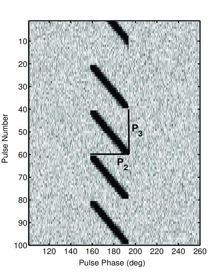
Figure 1: The schematic diagram for a stack of one hundred successive pulses of fake data, with pulse phase plotted horizontally and pulse number vertically. $P_{2}$ and $P_{3}$ are the separation of successive drift bands horizontally and vertically, respectively.

Nulling is when the pulsed emission abruptly switches off with duration ranging from one to many thousands of pulse periods and then abruptly resumes its normal flux density (Backer, 1970), and is thought to be magnetospheric in origin (Kramer et al., 2006; Wang et al., 2007; Timokhin, 2010). The phenomenon seems to occur at all frequencies and to all pulse components simultaneously, but partial nulls are also detected (Wang et al., 2007). A variety of models have been proposed for nulling, such as orbital companions (Cordes & Shannon, 2008), missing the line of sight (Herfindal & Rankin, 2007), switching between curvature radiation and inverse Compton scattering (Zhang et al., 1997) and magnetic field instability (Geppert et al., 2003).

Diverse patterns of transition between burst and null states have been observed in several pulsars. For PSR B0818$-$41 (Bhattacharyya et al., 2010) and PSR J1502$-$5653 (Li et al., 2012a), an abrupt rise of intensity when emission starts after a null and an exponential decay of pulse emission at the end of a burst are seen. On the other hand, an abrupt onset of nulling was observed from PSRs B0031$-$07 and J1738$-$2330 (Vivekanand, 1995; Gajjar et al., 2014).

Studies of pulsars that exhibit both nulling and drifting subpulses and the interaction between them provide insights into the properties of pulsar magnetospheres (Redman et al., 2005; Force & Rankin, 2010). Attempts have been made to unite the two phenomena (van Leeuwen et al., 2002, 2003; Jones, 2011) by examining more pulsars with similar behaviour. Smits et al. (2005) reported that transitions from one drift mode to another are interspersed with at least one null pulse. Different drift modes were also detected from PSR B0809+74, which exhibits transitions between two distinct modes after it goes through a null (van Leeuwen et al., 2002). PSR B1737+13 provides a unique opportunity to study the interactions between drifting subpulses and nulling behaviours with its two intensity modulation periods of 9 and 92 rotation periods, which suggest a subbeam carousel with 10 ’beamlets’ (Force & Rankin, 2010). Investigations of the on and off states for PSR B1931+24 which are accompanied by variations in spin-down rate show that nulling is a global property in pulsar magnetospheres (Kramer et al., 2006). Furthermore, studies (Lyne & Ashworth, 1983; van Leeuwen et al., 2002; Janssen & van Leeuwen, 2004; Redman et al., 2005) also revealed that the occurrence of nulls is not random and may be governed by emission cycles. Wang et al. (2007) showed the correlation of pulsar nulling and mode changing and proposed that those two emission properties may result from large-scale and persistent changes in the magnetospheric current re-distribution. Rankin & Wright (2003) pointed out that pulsar magnetosphere is a non-steady, and non-linear interactive system. So far nulling has been detected in almost 200 pulsars and the duration of a null and the interval between them appear random, although a correlation between the frequency of occurrence and the pulsar rotation period has been suggested (Ritchings, 1976). Despite these studies, however, a comprehensive understanding is still lacking and it is still unclear to what extent the two phenomena are related.

In this paper, we focus on PSR J1727$-$2739, which was discovered in the Parkes Multibeam Pulsar Survey (Hobbs et al., 2004), with measured rotational period of $P=1.29\ \rm{s}$ and first period derivative $\dot{P}=1.1\times 10^{-15}\ \rm{s\ s^{-1}}$, giving the characteristic age of $1.86\times 10^{7}\ \rm{yr}$ and the surface magnetic field of $10^{12}\ \rm{G}$, respectively (Hobbs et al., 2004). In Section 2, we describe the observations and detailed analysis of nulling and drifting subpulses for this pulsar. Examinations of the nulling and the properties of the bright states before and after the nulls, together with different modes of subpulse drift rates are also discussed. In section 3, we discuss several possible mechanisms for the phenomena and summarise our results.

2 Analysis and Results

The observations were made on 20 March, 2004 using the Parkes 64-m radio telescope in a frequency band centered at 1518 MHz. The data used for investigation of nulling behaviour are sampled every 250 $\mu$s for 2 hours and contain 5568 pulse periods. A more detailed description of the observing system is given by Wang et al. (2007). In order to increase signal-to-noise ratio, (S/N), the time series is averaged to 256 phase bins per pulse period. The average pulse profile, which is obtained by integrating across the data span, is illustrated in the lower panel of Fig. 2. Two steep-sided components with approximately equal amplitude are separated by $32\degr.0\pm 0\degr.7$ and are joined by a saddle region of emission.

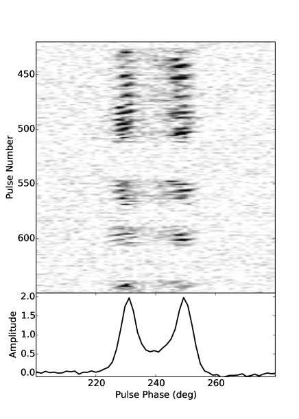
Figure 2: A sample of single pulse sequence in grey-scale intensities for PSR J1727$-$2739, in which increasing darkness represents higher intensity. Frequent nulling and subpulse drifting are observed. The pulse profile averaged over the whole data span is shown in the lower panel.

The upper panel of Fig. 2 shows a sample of single pulse data demonstrating both frequent nulling and complicated drifting subpulse phenomena. Instances of null states can easily be identified between pulse number 514 to 545, pulse number 570 to 587 and pulse number 608 to 638. For the burst state, strong pulses are clustered, between which short null intervals are seen. Analysis of the single-pulse sequences also reveals regions of drifting patterns with the variable drift rates. The drift rate at the leading region is steeper than that at the trailing region. On several occasions, the drifting at the trailing component becomes irregular, and for the first and last few active pulses the drift behaviour disappears, which indicates that it takes a few pulse periods for the drifting to establish and then cease before a null.

2.1 Nulling

Fig. 3 shows the time sequence of pulse energy for PSR J1727$-$2739 revealing many blocks of consecutive strong pulses separated by frequent nulling. The individual on-pulse energy was calculated by averaging the baseline-subtracted data in the on-pulse window and then scaling by the average value. The average off-pulse energy was measured in an equal number of off-pulse bins and then scaled by the same factor. We follow the similar procedure presented by Bhattacharyya et al. (2010) for identification of individual nulls, in which pulses with intensity smaller than $5\sigma_{ep}$ are classified as nulls, where $\sigma_{ep}$ is the uncertainty in the pulse energy calculated from the root-mean-square energy in the off-pulse window. Fig. 4 shows the on/off pulse time series for a section of the data with individual pulses classified as either null or burst states. In this work, a total of 53 blocks of burst state (2085 pulses) are identified for the whole observations. The durations of burst states vary from about 2 pulses to 133 pulses with a median duration of 28 pulses, although occasional individual strong pulses are also seen within (otherwise) null intervals. Null states last from about 6 pulses to 281 pulses with a median duration of 43 pulses.

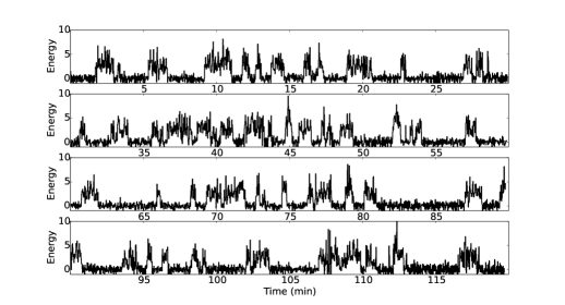
Figure 3: The two-hour evolution of relative pulse energy for PSR J1727$-$2739. The time sequence is equally divided into four panels, each presents half an hour of data.

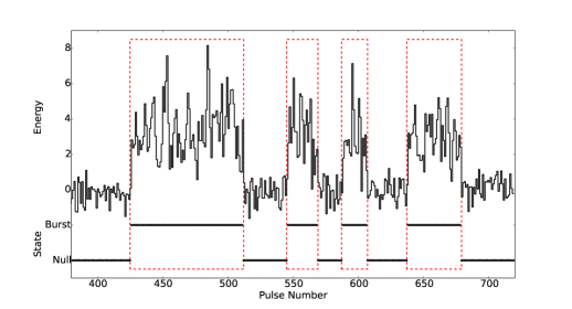
Figure 4: Upper part: On-pulse energy versus pulse number. For clarity, four identified burst states are enclosed in rectangular regions. The null or burst states are classified and shown in the lower part of figure.

The cryogenically-cooled receiver had a stable system temperature over two hours and the variation of the system gain is small, so we use uncalibrated data for our fluctuation analyses (Wang et al., 2007). Pulse energy distributions provide statistical information for the characterisation of pulsar nulling properties. Fig. 5 presents the energy distributions for the on-pulse windows and off-pulse windows. The off-pulse energy histogram shows a Gaussian shape centered around zero, while the broader on-pulse energy histogram has two Gaussian components corresponding to active and null pulses. These two histograms clearly overlap. Following the method described by Ritchings (1976), an increasing fraction of the off-pulse histogram centered on zero energy was subtracted from the observed on-pulse distribution until the sum of the difference counts in bins with $E<0$ was zero. The fraction determined in this way is the “null fraction” (NF) which is the fraction of the pulse sequence which is null. The uncertainty of NF is simply given by $\sqrt{n_{p}}/N$, where $n_{p}$ is the number of null pulses and N is the total number of observed pulses (Wang et al., 2007). The null fraction (NF) of this pulsar is estimated to be $68.2\pm 1.1\%$.

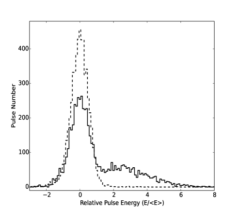
Figure 5: Energy histograms for the on-pulse windows (solid line) and off-pulse windows (dashed line). The energies are normalized by the mean on-pulse energy.

The identified contiguous null and burst lengths are shown in Fig. 6. It is obvious that the histogram of burst length peaks at around 20 pulse periods. For the short nulls, the histogram indicates that the distribution has a favor of around 5$-$35 periods. The decline of short nulls to long nulls may be fitted by a power-law distribution which has a slope of $\alpha=-1.0\pm 0.2$.

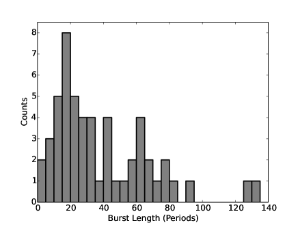
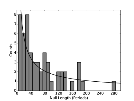
Figure 6: The distributions of duration of burst (left panel) and null (right panel) states. The histogram of null duration has an approximate power-law distribution with a slope of $\alpha=-1.0\pm 0.2$, as indicated with the solid curve in the right panel.

2.2 Pulse energy variations

Through a careful inspection of the null sequences, three examples of an isolated detectable pulse were found during null states, which means that, technically, ”bursts” can be as short as 1 pulse period. Also, detectable pulses were found in nominally null regions adjacent to burst regions. A ”guard band” of 1 pulse before and after burst regions was used to eliminate 31 of these transition pulses. After removing these 34 pulses, there is no obvious energy with S/N larger than 3 after integrating all 3449 null pulses, as shown in the lower panel of Fig. 7. The integrated pulse profile obtained from all 2119 burst pulses is shown in the upper panel.

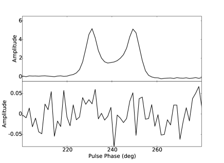
Figure 7: Integrated pulse profiles of PSR J1727$-$2739 for 2119 burst pulses (top panel) and the 3449 null pulses (bottom panel).

Investigation of the transitional patterns between burst and null states reveals different modes for the pulse energy changes. A zoom-in view of pulse energy for the pulses from 775 to 980 is presented in Fig. 8, during which two burst states are detected. It shows that the pulse intensity for the first few active pulses just after nulls increases relatively rapidly. However, the transitions from burst to null state shows two types of variation, either a gradual decline as seen in the first burst, or a more abrupt drop as seen in the second burst. These two transitional patterns are reported here for the first time for this pulsar.

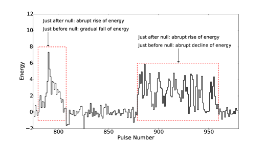
Figure 8: Zoom-in view for the on-pulse energy versus pulse number from pulse 775 to 980 showing the two types of burst decay.

The gradual rise at the onset of a burst and the slow decay from a burst to the null state are modeled by exponential functions (Lewandowski et al., 2004; Gajjar et al., 2014). The rise and fall times are derived from a least-square fit of an exponential function to the data and are defined as the time between the start point and the point where the function is 90 per cent or 10 per cent of the maximum, for the rise and fall respectively. Fig. 9 shows the resulting histograms for 48 burst states with high S/N burst pulses. The rise times are dominantly around six pulse periods, whereas a bi-modal distribution is found for the decay times, with a prominent peak at about three pulse periods and a second peak around 15 pulse periods.

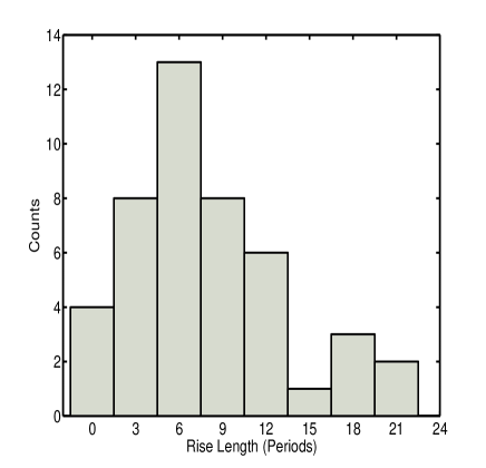
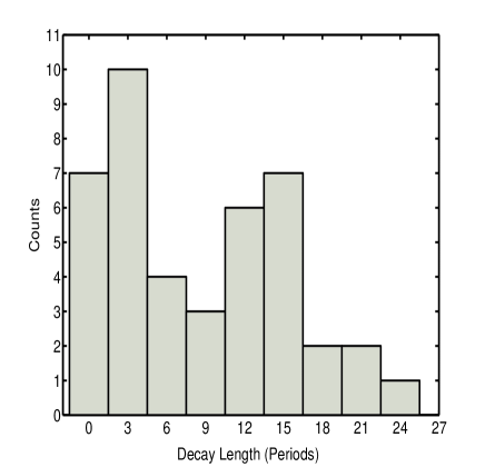
Figure 9: Histograms of rise time (left panel) and fall time (right panel) from exponential fits to pulse energies at the start and end of bursts.

Fig. 10 presents the average pulse profiles for the first active pulse (FAP, shown with the dash-dotted line) immediately after a null and the last active pulse (LAP, shown with the dashed line) just before a null respectively. Both profiles have double peaked components with similar pulse width, but the leading component is stronger than the trailing component for FAP, and vice verse for LAP. We applied the two-sample Kolmogorov-Smirnov (KS) test to the cumulative distribution functions of the FAP and LAP (Gajjar et al., 2014) and found an 83 per cent probability that the two profiles were drawn from the same distribution.

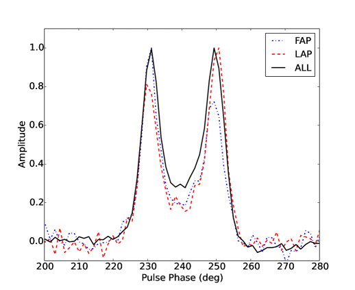
Figure 10: The pulse profiles averaged from the first active pulse (dash-dotted line) and last active pulse (dashed line) of the burst states. The solid line represents the average pulse profile of all pulses. They are normalized by their respective peak intensities for comparison.

2.3 Identification of two subpulse drift states

We used the phase-averaged power spectrum (hereafter PAPS) to analyse the data for drifting subpulses. This method is suitable for distinguishing drifting subpulses even when S/N is very low (Smits et al., 2005). The contour plots shown in the main panels of Fig. 11 and 12 are obtained from calculating the absolute values of Fourier transform for flux density at each fixed pulse phase across the pulse window. Subsequently, the PAPS is obtained by averaging the resulted transforms over pulse phase. A low-frequency modulation has been noted in numerous fluctuation studies and therefore the signals with frequency less than 0.05 cycles per rotational period (hereafter $c/P$) are set to 0 for clarity. In our data reduction, the resulting PAPS is plotted from 0 up to 0.5 $c/P$ with a frequency resolution given by the reciprocal of the length of the continuous pulse sequence. The width of 50 per cent of the peak is taken as the uncertainty corresponding to a probability of larger than 68.27%.

Figure 11 shows an example of the power spectrum of the flux as a function of pulse phase as well as the PAPS of a sequence of 30 pulses containing $10\ P$ periodicity. The PAPS peaks at $0.10\pm 0.02\ c/P$. We classify this as mode A drift. The fluctuation feature modulates all the emission in the leading and trailing region.

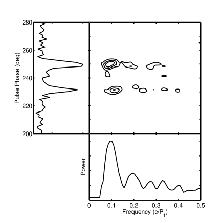
Figure 11: Contour plot for the power spectrum of the flux density as a function of pulse phase for a sequence of 30 pulses showing a 0.1 $c/P$ periodicity. The left-hand panel shows the power integrated over frequency. The bottom panel presents the power integrated over pulse phase. Signals at frequencies less than 0.05 $c/P$ have been set to 0.

Figure 12 shows the power spectrum for the flux density as a function of pulse phase as well as the PAPS for a sequence of 25 single pulses, containing $5\ P$ periodicity. The PAPS peaks at $0.21\pm 0.04\ c/P$. We classify this as mode B drift. It is noted that the modulation feature is predominant in the leading component.

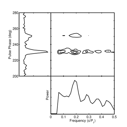
Figure 12: Same as in Fig. 11, but for another pulse sequence of length 25 pulse periods where a 0.2 $c/P$ periodicity is detected prominently in the first component.

An example of how fast the drift rate can change is shown in Fig. 13. As in Fig. 2, pulse number increases from top to bottom. Mode A drifting is seen in the first four drift bands, then within a few pulses, the drift switches to mode B without any null. In addition, the first few active pulses just after a null and the last few active pulses before a null show an irregular drifting pattern, whereas central pulses have a more normal drift pattern. This kind of transition in drift rates between burst and null states is seen throughout most of the data set.

A careful examination of the subpulse drifting in the two components reveals an irregular drifting in the trailing region (see pulses from number 475 to 500, which exhibit subpulse drifting in mode B) on several occasions, while the drifting in the leading region is generally regular. The irregular drifting in the trailing component is especially seen in Mode B and results in the weaker spectral feature seen in Fig. 12.

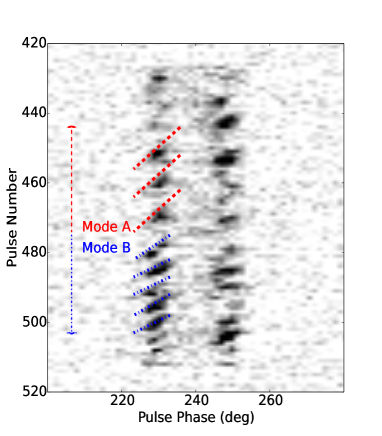
Figure 13: Grey-scale plot of individual pulses showing an example of the rapid change in drift mode from A to B within a few pulses. The two drift modes are indicated by the dashed lines.

2.4 Comparison of two drift modes

The periodicity of subpulse drifting is first checked visually from the single pulse sequence of each burst state. We then adjust the start and end of the sequence in order to achieve highest S/N of the PAPS peak. Finally, the location of the peak is determined as the drift frequency. Values of $\Delta\phi$ are determined by using the cross-correlation technique described by Smits et al. (2005) in which the correlation between consecutive pulses is fitted by a Gaussian curve. $P_{2}$ is then calculated by multiplying the mean phase drift by $P_{3}$.

The values of $P_{3}$ for all drifting sequences in the 5568 pulses are shown in Figure 14. The black rectangles indicate sequence of burst pulses without any detection of subpulse drifting, which we classify as mode C for convenience. The blank regions represent nulls. The two types of drifting subpulses are shown with blue and red bars. The transitions from one mode to the other can be very rapid in one or a few pulse periods with no intervening null. Table 1 summarises the occurence of the three modes and the drift parameters for modes A and B. The measured $P_{2}$ for drift mode A is larger than that for drift mode B by a factor of 1.43, unlike PSR B0031$-$07 where $P_{2}$ for the three different drift modes are the same (Huguenin et al., 1970; Smits et al., 2005).

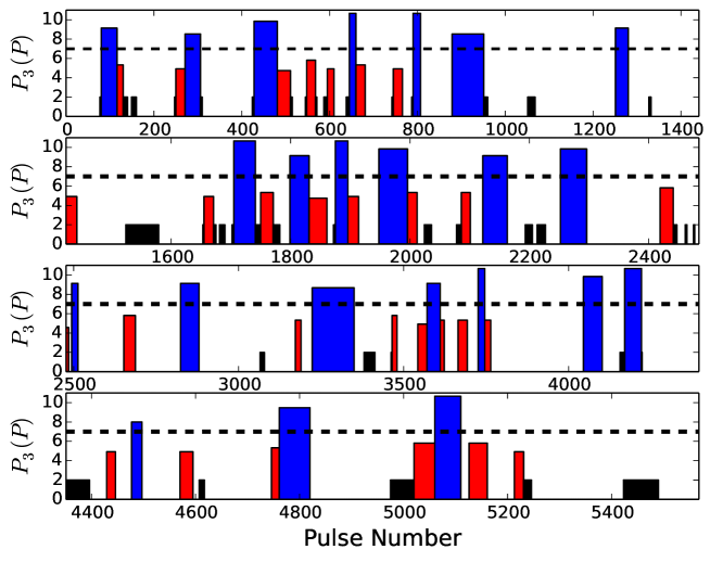
Figure 14: Sequences of burst states giving observed values of $P_{3}$. Modes A and B are shown with blue and red bars, and distinguished by the dashed lines. The black rectangles indicate bursts with no detection of subpulse drifting and the blank areas are nulls.

Table 1: List of average values for $P_{3}$, $\Delta\phi$, $P_{2}$, and widths of the average intensity profiles for different drift modes at 1518 MHz observed with Parkes radio telescope. The values of $P_{2}$ are derived from those of $P_{3}$ and $\Delta\phi$.

Drift	Number of	$P_{3}$	$\Delta\phi$	$P_{2}$	Number of	10% width	50% width
mode	sequences	($P$)	($\degr/P$)	($\degr$)	pulses	($\degr$)	($\degr$)
A	23	$9.7\pm 1.6$	$1.6\pm 0.3$	$15.6\pm 5.5$	1019	$29.8\pm 1.5$	$24.4\pm 1.5$
B	29	$5.2\pm 0.9$	$2.1\pm 0.3$	$10.9\pm 3.5$	609	$30.7\pm 1.5$	$25.0\pm 1.5$
C	40				457	$31.5\pm 1.5$	$24.6\pm 1.5$

Figure 15 presents three average profiles obtained from integrating pulses for each drift modes. The solid line shows the average profile of 1019 pulses containing subpulses with mode A drift, the dashed line shows the average profile of 609 pulses for mode B drift, and 457 pulses for mode C drift is presented with the dash-dotted line. The intensity of the leading and trailing components in drift modes A and B are almost the same. For mode C, with no subpulse drifting, the leading component is slightly stronger than the trailing component in intensity. KS-test comparisons between the average pulse profiles of the three modes suggest similar distributions with probabilities of 89% between A and C, 99% between B and C, and 89% between A and B. The last two columns in Table 1 give the widths of the average intensity profiles for different modes. The profile widths for the three drift modes are equal within the uncertainties.

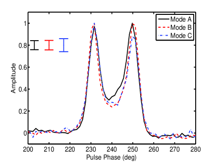
Figure 15: The average pulse profiles for mode A (solid line), mode B (dashed line) and mode C (dash-dotted line), with $3\sigma$ uncertainties determined from the off-pulse window.

Burst durations for each of the three different drift modes can be obtained from examination of the single pulse data using the above-mentioned method. Fig. 16 shows these distributions for the three drift modes, which can be compared with the overall distribution of burst duration given by the upper plot in Fig. 6. On average, mode A bursts have longer durations than mode B bursts, and mode C bursts have the shortest durations, with about 90 per cent of mode C bursts having a duration of less than 20 pulse periods.

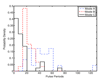
Figure 16: Distributions of burst durations for the three modes.

3 Discussion and Conclusions

We report new results on the properties of nulling and drifting subpulses for pulsar J1727$-$2739 based on detailed analysis of 5568 pulse periods observed at centre frequency 1518 MHz using the Parkes 64-m radio telescope. Nulls are detected, with durations of 6 to 281 pulse periods and an average null fraction of about 68%. Burst durations range from 2 to 133 pulses, although occasional isolated pulses are seen in otherwise null intervals. The intensity of most bursts immediately after nulls is observed to rise to near maximum in about six pulse periods, whereas the transition from bursts to nulls exhibits two types of decay, either gradual or rapid. Emission observed from the pulse profile averaged over all null pulses reveals no pulsed emission with S/N greater than 3. Analysis on the shape of the average profiles for last active pulses (LAP) and first active pulses (FAP) reveal that they both have two components and the same overall width, but LAP show a stronger trailing component and opposite for FAP. This is inconsistent with previous studies which suggested similarities between LAP and FAP (Vivekanand, 1995). The observed differences between LAP and FAP from J1727$-$2739 suggest that the emission conditions are different at the start and end of bursts.

We demonstrate that PSR J1727$-$2739 exhibits drifting subpulses of two distinct modes with characteristic ${P_{3}}$ of $9.7\pm 1.6P$ (mode A) and $5.2\pm 0.9P$ (mode B), together with mode C in which no drifting subpulses are detected. The occurrence rate was 49% for mode A, 29% for mode B and 22% for mode C as shown in Fig. 16. Our results also show that transitions between different modes occur either rapidly within a few pulses or are split by nulls. The onset and ending pulses in the burst states show irregular drift properties, and occasional irregular drifting patterns are observed in the trailing component. Furthermore, the average pulse profiles for modes A and B are similar with nearly equal components, but for mode C the leading component is stronger.

Fig. 14 shows that some transitions between drift modes are rapid within a burst, while others transition after a null. This contrasts with PSRs B0809+74 and B0031$-$07 where changes in the drift pattern normally occur in association with a null. This implies that for PSR J1727$-$2739 the nulls and the disordered drift mode C do not act as so-called ‘reset phases’ (Rankin et al., 2013). However, the drift rate reduces to zero near the onset and the end of most burst states. Cross-correlation analyses between drift rate and average intensity and burst duration showed no significant correlations.

A modified model based on the traditional vacuum gap model (Ruderman & Sutherland, 1975) was proposed by Gil et al. (2003) with partial outflow of thermal ions or electrons from the polar cap along with the magnetospheric electron-positron pair plasma production. The conductivity increases towards the end of the burst, with enough charged particles in the accelerating gap to decrease the electric field to a stable value where the radio emission is still active but the drift rate goes off. With more accumulation, the acceleration gap will not survive and thus the radio emission ceases. The two patterns of decay and the abrupt rise in pulse intensity before and after a null also suggests different magnetospheric states in the magnetosphere (Lyne et al., 2010; Melrose & Yuen, 2014). Switching between two different magnetospheric states may result in the transitions between bursts and null states, and the exponential gradual decay may be interpreted as slow relaxation from one state to another. Wang et al. (2007) suggested that emission can cease or commence suddenly when the charge or magnetic configuration in the magnetosphere reaches a so-called ‘tipping point’ but the triggering mechanism is unknown.

The different observed subpulse drift modes suggest possible variations in the emitting properties and may be an indication of a local change in the electromagnetic field configuration in the gap. Subpulses at different heights within same magnetic flux tube will experience different plasma flow rates (van Leeuwen et al., 2003) resulting in different drift modes. Another model by Smits et al. (2005) suggests that groups of subpulses in different drift modes are located in different concentric radiating rings and emitted from different magnetic field lines. In this model, plasma at inner field lines relative to the magnetic axis will experience greater electric potential giving faster drift and stronger radio emission. Changes in drift mode result from shifting of emission between different field lines. Thus both models predict narrower average pulse profile for drift mode with emission that comes from closer to the magnetic axis. However, the equal observed pulse widths in the two drift modes implies that emission does not shift relative to the magnetic axis. For magnetospheric plasma of resistive nature (Li et al., 2012b), where the differential rotation of plasma is responsible for the drifting emission in phase and the conductivity determines the observed subpulse drifting features, mode B may correspond to a faster ${\bf E}\times{\bf B}$ drift and stronger emission because of larger conductivity. However, as for the transitions between nulling and burst states, the trigger mechanism for variations of conductivity is still unclear.

Our results show that the time-scale for the change of the magnetospheric current varies from several to dozens pulse periods, and it is not yet clear as to how the emitted pulses are modulated in intensity and in phase by the switching process of the magnetospheric currents and the electric field. To the best of our knowledge, no model can explain the observed features satisfactorily. It is difficult to draw a definitive conclusion on the interaction between nulling and switching of different subpulse drift modes. To continue this study, we would require multi-frequency simultaneous single pulse observations with full Stokes parameters to reveal more detailed information on the variations of the size and location of the active region.