Efficient and Compact Representations of Some Non-Canonical Prefix-Free Codes

Abstract

For many kinds of prefix-free codes there are efficient and compact alternatives to the traditional tree-based representation. Since these put the codes into canonical form, however, they can only be used when we can choose the order in which codewords are assigned to symbols. In this paper we first show how, given a probability distribution over an alphabet of $\sigma$ symbols, we can store an optimal alphabetic prefix-free code in $\mathcal{O}\!\left({\sigma\lg L}\right)$ bits such that we can encode and decode any codeword of length $\ell$ in $\mathcal{O}\!\left({\min(\ell,\lg L)}\right)$ time, where $L$ is the maximum codeword length. With $\mathcal{O}\!\left({2^{L^{\epsilon}}}\right)$ further bits, for any constant $\epsilon>0$, we can encode and decode $\mathcal{O}\!\left({\lg\ell}\right)$ time. We then show how to store a nearly optimal alphabetic prefix-free code in $o(\sigma)$ bits such that we can encode and decode in constant time. We also consider a kind of optimal prefix-free code introduced recently where the codewords’ lengths are non-decreasing if arranged in lexicographic order of their reverses. We reduce their storage space to $\mathcal{O}\!\left({\sigma\lg L}\right)$ while maintaining encoding and decoding times in $\mathcal{O}\!\left({\ell}\right)$. We also show how, with $\mathcal{O}\!\left({2^{\epsilon L}}\right)$ further bits, we can encode and decode in constant time. All of our results hold in the word-RAM model.

1 Introduction

Prefix-free codes are a fundamental tool in data compression; they are used in one form or another in almost every compression tool. Prefix-free codes allow assigning variable-length codewords to symbols according to their probabilities in a way that the encoded stream can be decoded unambiguously [2, Ch. 5]. Their best-known representative, Huffman codes [3], yield the optimal encoded file size for a given probability distribution. Fast encoding and decoding algorithms for prefix-free codes are then of utmost relevance. When the source alphabet is large (e.g., in word-based natural language compression [4, 5], East Asian or numeric alphabets) or when the text is short compared to the alphabet (e.g., for compression boosting [6] or adaptive compression [7]), a second concern is the space spent in storing the codewords of all the source symbols, because it could outweigh the compression savings.

The classical encoding and decoding algorithms for a codeword of length $\ell\leq L$ take in the word-RAM model $\mathcal{O}\!\left({1}\right)$ and $\mathcal{O}\!\left({\ell}\right)$ time, respectively, using $\mathcal{O}\!\left({\sigma L}\right)$ bits of space, where $\sigma$ is the size of the source alphabet and $L$ is the maximum codeword length. For encoding we just store each codeword in plain form, whereas for decoding we use a binary tree $\mathcal{B}$ where each leaf corresponds to a symbol and the path from the root to the leaf spells out its code, if we interpret going left as a $0$ and going right as a $1$. Faster decoding is possible if we use the so-called canonical codes, where the leaves are sorted left-to-right by depth, and by symbol upon ties [8]. Canonical codes enable $\mathcal{O}\!\left({\lg L}\right)$-time encoding and decoding while using $\mathcal{O}\!\left({\sigma\lg\sigma}\right)$ bits of space, again in the word-RAM model. In theory, both encoding and decoding can be done even in constant time with canonical codes [9].

Both the original and the canonical Huffman codes achieve optimality by reordering the leaves as necessary. There are applications for which the codes must be so-called alphabetic, that is, the leaves must respect, left-to-right, the alphabetic order of the source symbols. This allows lexicographically comparing strings directly in compressed form, which enables lexicographic data structures on the compressed strings [10, 11] and compressed data structures that represent point sets as sequences of coordinates [12]. Optimal alphabetic (prefix-free) codes achieve codeword lengths close to those of Huffman codes [13]. Interestingly, since the mapping between symbols and leaves is fixed, alphabetic codes need only store the topology of the binary tree $\mathcal{B}$ used for decoding, which can be represented more succinctly than optimal prefix-free codes, in $\mathcal{O}\!\left({\sigma}\right)$ bits [14], so that encoding and decoding can still be done in time $\mathcal{O}\!\left({\ell}\right)$ [9]. As far as we know, there are no equivalents to the fast and compact representations of canonical codes for alphabetic codes.

There are other cases where canonical prefix-free codes cannot be used. Wavelet matrices, for example, serve as compressed representations of discrete grids and sequences over large alphabets [15]. They are compressed with an optimal prefix-free code where the codewords’ lengths are non-decreasing if arranged in lexicographic order of their reverses. They represent the code in $\mathcal{O}\!\left({\sigma L}\right)$ bits, and encode and decode a codeword of length $\ell$ in time $\mathcal{O}\!\left({\ell}\right)$.

Our contributions

In Section 3 we show how, given a probability distribution, we can store an optimal alphabetic prefix-free code in $\mathcal{O}\!\left({\sigma\lg L}\right)$ bits such that we can encode and decode any codeword of length $\ell$ in $\mathcal{O}\!\left({\min(\ell,\lg L)}\right)$ time. This time decreases to $\mathcal{O}\!\left({\lg\ell}\right)$ if we use $\mathcal{O}\!\left({2^{L^{\epsilon}}}\right)$ additional bits, for any constant $\epsilon>0$. We then show in Section 4 how to store a nearly optimal alphabetic prefix-free code in $o(\sigma)$ bits such that we can encode and decode in constant time. These, and all of our results, hold in the word-RAM model.

In Section 5 we consider the optimal prefix-free codes used for wavelet matrices [15]. We show how to store such a code in $\mathcal{O}\!\left({\sigma\lg L}\right)$ bits and still encode and decode any symbol in $\mathcal{O}\!\left({\ell}\right)$ time. We also show that, using $\mathcal{O}\!\left({2^{\epsilon L}}\right)$ further bits, we can encode and decode in constant time. Our first variant is simple enough to be implementable. Our experiments show that on large alphabets it uses 20–30 times less space than a classical implementation, at the price of being 10–20 times slower at encoding and 10–30 at decoding.

An early version of this paper appeared in Proc. SPIRE 2016 [1]. This extended version includes much more detailed explanations as well as new results for fast encoding and decoding of optimal alphabetic codes (Section 3).

2 Basic Concepts

2.1 Assumptions

Our results hold in the word-RAM model, where the computer word has $w$ bits and all the basic arithmetic and logical operations can be carried out in constant time. We assume for simplicity that the maximum codeword length is $L=\mathcal{O}\!\left({w}\right)$, so that any codeword can be accessed in $\mathcal{O}\!\left({1}\right)$ time. We assume binary codewords, which are the most popular because they provide the best compression, though our results generalize to larger alphabets.

We generally express the space in bits, but when we say $\mathcal{O}\!\left({x}\right)$ space, we mean $\mathcal{O}\!\left({x}\right)$ words of space, that is, $\mathcal{O}\!\left({xw}\right)$ bits.

By $\lg$ we denote the logarithm to the base $2$ by default.

2.2 Basic data structures

Predecessors

This predecessor problem consists in building a data structure on the integers $0\leq x_{1}<x_{2}<\cdots<x_{n}<U$ such that later, given an integer $y$, we return the largest $i$ such that $x_{i}\leq y$. In the RAM model, with $\lg U=\mathcal{O}\!\left({w}\right)$, it can be solved with structures using $\mathcal{O}\!\left({n\lg U}\right)$ bits in $\mathcal{O}\!\left({\lg\lg U}\right)$ time, as well as in $\mathcal{O}\!\left({\lg_{w}n}\right)$ time, among other tradeoffs [16]. It is also possible to find the answer in time $\mathcal{O}\!\left({\lg i}\right)$ using exponential search.

Bitmaps

A bitmap $B[1..n]$ is an array of $n$ bits that supports two operations: $rank_{b}(B,i)$ counts the number of bits $b\in\{0,1\}$ in $B[1..i]$, and $select_{b}(B,j)$ gives the position of the $j$th $b$ in $B$ (we use $b=1$ by default). Both operations can be supported in constant time if we store $o(n)$ bits on top of the $n$ bits used for $B$ itself [17, 18]. When $B$ has $m$ $1$s and $m\ll n$ or $n-m\ll n$, it can be represented in compressed form, using $m\lg(n/m)+O(m+n/\lg^{c}n)$ bits in total for any $c$, so that $rank$ and $select$ are supported in time $O(c)$ [19]. All these results require the RAM model of computation with $\lg n=\mathcal{O}\!\left({w}\right)$.

Variable-length arrays

An array storing $n$ nonempty strings of lengths $l_{1},l_{2},$ $\ldots,l_{n}$ can be stored by concatenating the strings and adding a bitmap of the same length of the concatenation, $B=1\,0^{l_{1}-1}~{}1\,0^{l_{2}-1}\cdots 1\,0^{l_{n}-1}$. We can then determine in constant time that the $i$th string lies between positions $select(B,i)$ and $select(B,i+1)-1$ in the concatenated sequence.

Wavelet trees

A wavelet tree [20] is a binary tree used to represent a sequence $S[1..n]$, which efficiently supports the queries $access(S,i)$ (the symbol $S[i]$), $rank_{c}(S,i)$ (the number of symbols $c$ in $S[1..i]$), and $select_{c}(S,j)$ (the position of the $j$th occurrence of symbol $c$ in $S$). In this paper we use a wavelet tree variant [21] that uses $n\lg s\,(1+o(1))+\mathcal{O}\!\left({s\lg n}\right)$ bits, where the alphabet of $S$ is $\{1,\ldots,s\}$, and supports the three operations in time $\mathcal{O}\!\left({1+\lg s/\lg w}\right)$.

2.3 Prefix-free codes

A prefix-free code (or instantaneous code) is a mapping from a source alphabet, of size $\sigma$, to a sequence of bits, so that each source symbol is assigned a codeword in a way that no codeword is a prefix of any other. A sequence of source symbols is then encoded as a sequence of bits by replacing each source symbol by its codeword. Compression can be obtained by assigning shorter codewords to more frequent symbols [2, Ch. 5]. When the code is prefix-free, we can unambiguously determine each original symbol from the concatenated binary sequence, as soon as the last bit of the symbol’s codeword is read. An optimal prefix-free code minimizes the length of the binary sequence and can be obtained with the Huffman algorithm [3].

For constant-time encoding, we can just store a table of $\sigma L$ bits, where $L$ is the maximum codeword length, where the codeword of each source symbol is stored explicitly using standard bit manipulation of computer words [22, Sec. 3.1]. Since $L=\mathcal{O}\!\left({w}\right)$, we have to write only $\mathcal{O}\!\left({1}\right)$ words per symbol. Decoding is a bit less trivial. The classical solution for decoding a prefix-free code is to store a binary tree $\mathcal{B}$, where each leaf corresponds to a source symbol and each root-to-leaf path spells the codeword of the leaf, if we write a $0$ whenever we go left and a $1$ whenever we go right. Unless the code is obviously suboptimal, every internal node of $\mathcal{B}$ has two children and thus $\mathcal{B}$ has $\mathcal{O}\!\left({\sigma}\right)$ nodes. Therefore, it can be represented in $\mathcal{O}\!\left({\sigma\lg\sigma}\right)$ bits, which also includes the space to store the source symbols assigned to the leaves. By traversing $\mathcal{B}$ from the root and following left or right as we read a $0$ or a $1$, respectively, we arrive in $\mathcal{O}\!\left({\ell}\right)$ time at the leaf storing the symbol that is encoded with $\ell$ bits in the binary sequence.

Since $\lg\sigma\leq L<\sigma$, the above classical solution takes $\mathcal{O}\!\left({\sigma L}\right)$ bits of space. We can reduce the space to $\mathcal{O}\!\left({\sigma\lg\sigma}\right)$ bits by deleting the encoding table and adding instead parent pointers to $\mathcal{B}$, so that from any leaf we can extract the corresponding codeword in reverse order. Both encoding and decoding take $\mathcal{O}\!\left({\ell}\right)$ time in this case.

Figure 1 shows an example of Huffman coding.

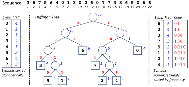
Figure 1: An example of Huffman coding. A sequence of symbols on top, the symbol frequencies on the left, the Huffman tree $\mathcal{B}$ in the center, and the corresponding codewords on the right. The blue numbers on the tree nodes show the total frequencies in the subtrees. The sequence uses $n\lg\sigma=66$ bits in plain form, but $61$ bits in Huffman-compressed form.

2.4 Canonical prefix-free codes

By the Kraft Inequality [23], we can put any prefix-free code into canonical form [8] while maintaining all the codeword lengths. In the canonical form, the leaves of lower depth are always to the left of leaves of higher depth, and leaves of the same depth respect the lexicographic order of the source symbols, left to right.

Canonical codes enable faster encoding and decoding, and/or lower space usage. Moffat and Turpin [24] give practical data structures that can encode and decode a codeword of $\ell$ bits in time $\mathcal{O}\!\left({\lg\ell}\right)$. Apart from the $\mathcal{O}\!\left({\sigma\lg\sigma}\right)$ bits they use to store the symbols at the leaves, they need $\mathcal{O}\!\left({L^{2}}\right)$ bits for encoding and decoding; they do not store the binary tree $\mathcal{B}$ explicitly. They use the $\mathcal{O}\!\left({\sigma\lg\sigma}\right)$ bits to map from a symbol $c$ to its left-to-right leaf position $p$ and back. Given the increasing positions and codewords of the leftmost leaves of each length, they find the codeword of a given leaf position $p$ by finding the predecessor position $p^{\prime}$ of $p$, and adding $p-p^{\prime}$ to the codeword of $p^{\prime}$, interpreted as a binary number. For decoding, they extend all those first codewords of each length to length $L$, by padding them with $0$s on their right. Then, interpreting the first $L$ bits of the encoded stream as a number $x$, they find the predecessor $x^{\prime}$ of $x$ among the padded codewords, corresponding to leaf position $p^{\prime}$. The leaf position of the encoded source symbol is then $p^{\prime}+(x-x^{\prime})/2^{L-\ell}$, where $\ell$ is the depth of the leaf $p$. This is also used to advance by $\ell$ bits in the encoded sequence. The time $\mathcal{O}\!\left({\lg\ell}\right)$ is obtained with exponential search (binary search would yield $\mathcal{O}\!\left({\lg L}\right)$); the other predecessor time complexities also hold.

Figure 2 continues our example with a canonical Huffman code.

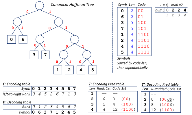
Figure 2: The canonical code corresponding to Figure 1. To encode a symbol, the table $E$ gives its leaf rank $p$, whose predecessor $p^{\prime}$ we find in the ranks of table $T$, together with its length $\ell$. We then add $p-p^{\prime}$ to the codeword associated with $p^{\prime}$. To decode $x$, a predecessor search for $x$ on the padded codewords of $T^{\prime}$ finds $x^{\prime}$. Its associated length $\ell$ and leaf position $p^{\prime}$ are in $T$. We use them to obtain the entry in $D$ storing the symbol.

Gagie et al. [9] improve upon this scheme both in space and time, by using more sophisticated data structures. They show that, using $\mathcal{O}\!\left({\sigma\lg L+L^{2}}\right)$ bits of space, constant-time encoding and decoding is possible.

2.5 Alphabetic codes

A prefix-free code is alphabetic if the codewords (regarded as binary strings) maintain the lexicographic order of the corresponding source symbols. If we build the binary tree $\mathcal{B}$ of such a code, the leaves enumerate the source symbols in order, left to right. Hu and Tucker [13] showed how to build an optimal alphabetic code, whose codewords are at most one bit longer than the optimal prefix-free codes on average [2].

Figure 3 gives an alphabetic code tree for our running example.

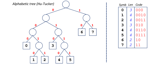
Figure 3: An alphabetic code corresponding to the frequencies of Figure 1. The compressed sequence is $62$ bits long.

In an alphabetic code we do not need to map from symbols to leaf positions, so the sheer topology of $\mathcal{B}$ is sufficient to describe the code. Such a topology can be described in $\mathcal{O}\!\left({\sigma}\right)$ bits, in a way that the tree navigation operations can be simulated in constant time, as well as obtaining the left-to-right position of a given leaf and vice versa [14]. With such a representation, we can then simulate the $\mathcal{O}\!\left({\ell}\right)$ encoding and decoding algorithms described in Section 2.3 [9].

On the other hand, there is no such a thing like a canonical alphabetic code, because the leaf left-to-right order cannot be altered. Indeed, no faster encoding and decoding algorithms exist for alphabetic codes. Our first contribution, in Sections 3 and 4, is a data structure of $\mathcal{O}\!\left({\sigma\lg L}\right)$ bits that encodes and decodes in time $\mathcal{O}\!\left({\min(\ell,\lg L)}\right)$, and even $\mathcal{O}\!\left({\lg\ell}\right)$ if we spend $\mathcal{O}\!\left({2^{L^{\epsilon}}}\right)$ further bits, for any constant $\epsilon>0$. While this increases the space compared to the $\mathcal{O}\!\left({\sigma}\right)$-bit basic structure, we show that $o(\sigma)$ bits of space are sufficient to encode and decode in constant time, if we let the average codeword length increase by a factor of $1+\mathcal{O}\!\left({1/\sqrt{\lg\sigma}}\right)$ over the optimal.

2.6 Codes for wavelet matrices

Claude et al. [15] showed how to build an optimal prefix-free code such that all the codewords of length $\ell$ come before the prefixes of length $\ell$ of longer codewords in the lexicographic order of the reversed binary strings. Specifically, they first build a classical Huffman code and then use the Kraft Inequality to build another code with the same codeword lengths and with the desired property. They store an $\mathcal{O}\!\left({\sigma L}\right)$-bit mapping between symbols and their codewords, which allows them to encode and decode codewords of length $\ell$ in time $\mathcal{O}\!\left({\ell}\right)$. They use such codes to compress wavelet matrices, which are data structures aimed to represent sequences on large alphabets. Thus, it is worthwhile to devise more space economical codeword representations.

Figure 4 gives a code tree of this type for our running example.

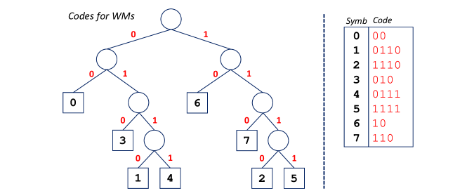
Figure 4: A code for wavelet matrices corresponding to the frequencies of Figure 1.

Our second contribution, in Section 5, is a representation for these codes that uses $\mathcal{O}\!\left({\sigma\lg L}\right)$ bits, with the same $\mathcal{O}\!\left({\ell}\right)$ encoding and decoding time. With $\mathcal{O}\!\left({2^{\epsilon L}}\right)$ further bits, for any constant $\epsilon>0$, we achieve constant encoding and decoding time.

3 Optimal Alphabetic Codes

In this section we consider how to efficiently store alphabetic (prefix-free) codes; recall Section 2.5. We describe a structure called BSD [25], and then how we use it to build our fast and compact data structures to store optimal alphabetic codes. We finally show how to make it faster using more space.

3.1 Binary Searchable Dictionaries (BSD)

Gupta et al. [25] describe a structure called BSD, which encodes $n$ binary strings of length $L$ using a trie that is analogous to the binary tree $\mathcal{B}$ we described above to store the code (except that here all the strings have the same length $L$). Let us say that the identifier of a string is its lexicographic position, that is, the left-to-right position of its leaf in the trie. Their structure supports extraction of the $i$th string (which is equivalent to our encoding), and fast computation of the identifier of a given string (which is equivalent to our decoding), both in $\mathcal{O}\!\left({\lg n}\right)$ time.

To achieve this, Gupta et al. define a complete binary search tree $T$ on the strings with lexicographic order (do not confuse $T$ with the binary trie; there is one node in $T$ per trie leaf). The complete tree can be stored without pointers. Each node $v$ of $T$ represents a string $v.x$, which is not explicitly stored. Instead, it stores a suffix $v.t=v.x[l+1..L]$, where $l$ is the length of the longest prefix $v.x$ shares with some $u.x$, over the ancestors $u$ of $v$ in $T$. For the root $v$ of $T$ it holds that $v.x=v.t$.

For both operations, we descend in $T$ until reaching the desired node. We start at the root $v$ of $T$, where we know $v.x$. The invariant is that, as we descend, we know $v.x$ for the current node $v$ and $u.x$ for all of its ancestors $u$ in $T$ (which we have traversed). Further, we keep track of the most recent ancestors $u.l$ and $u.r$ from where our path went to the left and to the right, respectively, and therefore it holds that $u=u_{l}$ if $v.t[1]=0$ and $u=u_{r}$ if $v.t[1]=1$ [25]. Whenever we choose the child $v^{\prime}$ of $v$ to follow, we compute $v^{\prime}.x$ by composing $v^{\prime}.x=u.x[1..L-|v^{\prime}.t|]\cdot v^{\prime}.t$, which restores the invariant. The procedure ends after $\mathcal{O}\!\left({\lg n}\right)$ constant-time steps, and we can do the concatenation that computes $v^{\prime}.x$ in constant time in the RAM model.

To extract the $i$th string, we navigate from the root towards the $i$th node of $T$. Because $T$ is a complete binary search tree, we know algebraically whether the $i$-th node is $v$, or it is to the left or to the right of $v$. If it is $v$, we already know $v.x$, as explained, and we are done. Otherwise, we choose the proper child $v^{\prime}$ of $v$ and continue the search. Finding $i$ from its string $x$ is analogous, except that we compare $x$ with $v.x$ numerically (in constant time in the RAM model) to determine whether we have found $v$ or we must go left or right. Because $T$ is complete, we know algebraically the identifier $v.i$ of each node $v$ without need of storing it.

Gupta et al. [25] show that, surprisingly, the sum of the lengths of all the strings $v.t$ is bounded by the number of edges in the trie. Our data structure for optimal alphabetic codes builds on this BSD data structure.

3.2 Our data structure

Given an optimal alphabetic code over a source alphabet of size $\sigma$ with maximum codeword length $L$, we store the lengths of the $\sigma$ codewords using $\sigma\lceil\lg L\rceil$ bits, and then pad the codewords on the right with 0s up to length $L$. We divide the lexicographically sorted padded codewords into blocks of size $L$ (the last block may be smaller). We collect the first padded codeword of every block in a predecessor data structure, and store all the (non-padded) codewords of each block in a BSD data structure, one per block.

The predecessor data structure then stores $\lceil\sigma/L\rceil$ numbers in a universe of size $2^{L}$. As seen in Section 2.2, the structure uses $\mathcal{O}\!\left({(\sigma/L)\lg(2^{L})}\right)=\mathcal{O}\!\left({\sigma}\right)$ bits and answers predecessor queries in time $\mathcal{O}\!\left({\lg\lg(2^{L})}\right)=\mathcal{O}\!\left({\lg L}\right)$.

Each BSD structure, on the other hand, stores (at most) $L$ strings $v.t$. Unlike the original BSD structure, our codewords are of varying length (those lengths were stored separately, as indicated). This does not invalidate the argument that the sum of the strings $v.t$ adds up to the number of edges in the trie of the $L$ codewords: what Gupta et al. [25, Lem. 3] show is that each edge of the trie is mentioned in only one string $v.t$, with no reference to the code lengths. We vary its encoding, though: We store all the strings $v.t$ of the BSD, in the same order of the nodes of $T$, concatenated in a variable-length array as described in Section 2.2. With constant-time $select$ we find where is $v.t$ in the concatenation, and with another $\mathcal{O}\!\left({1}\right)$ time we extract it in the RAM model.

Considering the extra space needed to find in constant time where is $v.t$, we spend $\mathcal{O}\!\left({1}\right)$ bits per trie edge. Since the trie stores up to $L$ consecutive leaves of the whole binary tree $\mathcal{B}$ (and internal nodes of $\mathcal{B}$ have two children because the alphabetic code is optimal), it follows that the trie has $\mathcal{O}\!\left({L}\right)$ nodes: There are $\mathcal{O}\!\left({L}\right)$ trie nodes with two children because there are $L$ leaves in the trie, and the trie nodes with one child are those leading to the leftmost and rightmost trie leaves. Since the leaves are of depth $L$, there are $\mathcal{O}\!\left({L}\right)$ of those trie nodes too. Therefore, we use $\mathcal{O}\!\left({L}\right)$ bits per BSD structure, adding up to $\mathcal{O}\!\left({\sigma}\right)$ bits overall.

The total space is then dominated by the $\sigma\lg L+\mathcal{O}\!\left({\sigma}\right)$ bits spent in storing the lengths of the codewords. On top of that, the predecessor data structure uses $\mathcal{O}\!\left({\sigma}\right)$ bits and the BSD structures use other $\mathcal{O}\!\left({\sigma}\right)$ bits.

To encode symbol $i$, we go to the $\lceil i/L\rceil$th BSD structure and find the $i^{\prime}$th string inside it, with $i^{\prime}=i-(\lceil i/L\rceil-1)\cdot i$. The algorithm is identical to that for BSD, except that each $v.x$ has variable length; recall that we have those lengths $|v.x|$ stored explicitly. We thus update $v^{\prime}.x=u.x[1..|v^{\prime}.x|-|v^{\prime}.t|]\cdot v^{\prime}.t$ when moving to node $v^{\prime}$.

To decode, we store in a number $x$ the first $L$ bits of the stream, find its predecessor in our structure, and decode $x$ in the corresponding BSD structure. The only difference is that, when we compare $x$ with $v.x$, their lengths differ (because we do not know the length $\ell$ of the codeword we seek, which prefixes $x$). Since the code is prefix-free, it follows that the codeword we look for is $v.x$ if $v.x=x[1..|v.x|]$, otherwise we go left or right according to which is smaller between those $|v.x|$-bit numbers. When we find the proper node $v$, the source symbol is the position $i$ of $v$ (which we compute algebraically, as explained) and the length of the codeword is $\ell=|v.x|$.

In both cases, the time is $\mathcal{O}\!\left({\lg L}\right)$ to find the proper node in the BSD plus, in the case of decoding, $\mathcal{O}\!\left({\lg L}\right)$ time for the predecessor search. As before, we can also encode and decode a codeword of length $\ell$ in time $\mathcal{O}\!\left({\ell}\right)$ using the basic $\mathcal{O}\!\left({\sigma}\right)$-bit representation. We can even choose the smallest by attempting the encoding/decoding up to $\lg L$ steps, and then switch to the $\mathcal{O}\!\left({\lg L}\right)$-time procedure if we have not yet finished.

Theorem 1

Given a probability distribution over an alphabet of $\sigma$ symbols, we can build an optimal alphabetic prefix-free code and store it in $\sigma\lg L+\mathcal{O}\!\left({\sigma}\right)$ bits, where $L$ is the maximum codeword length, such that we can encode and decode any codeword of length $\ell$ in $\mathcal{O}\!\left({\min(\ell,\lg L)}\right)$ time. The result assumes a $w$-bit RAM computation model with $L=\mathcal{O}\!\left({w}\right)$.

Figure 5 shows our structure for the codewords tree of Figure 4. Note that, for each BSD structure, the length of the concatenated strings $v.t$ equals the number of edges in the corresponding piece of the codewords tree. For example, to encode the symbol 3, we must encode the 4th symbol of $BSD_{1}$. We start at the root $u$ (corresponding to symbol 2), with $u.x=u.t=0011$. We know algebraically that the root corresponds to the 3rd symbol, so we go right to $v$, the node representing the symbol 3. Since $v.t[1]=1$, $v.t$ is encoded with respect to the nearest ancestor where we went right, that is, from the root $u$. We have $|v.x|=3$ stored explicitly, so we build $v.x=u.x[1..|v.x|-|v.t|]\cdot v.t=0\cdot 10$. Since we know algebraically that we arrived at the 4th symbol, we are done: the codeword for 3 is $010$. Let us now decode $0110=6$. The predecessor search tells it appears in $BSD_{2}$. We start at the root $u$ (which encodes 6). Since its extended codeword, $u.x=10\cdot 00$, is larger than $0110$, we go left to the node $v$ that represents 5. Since $v.t[1]=0$, $v.t$ is represented with respect to the last ancestor where we went left, that is, $u$. So we compose $v.x=u.x[1..|v.x|-|v.t|]\cdot v.t=\cdot 0111$. Now, since $v.x=0111$ is larger than our codeword $0110$, we again go left to the node $v^{\prime}$ that represents 4. Since $v^{\prime}.t[1]=0$, $v^{\prime}.t$ is also represented with respect to the last node where we went left, that is, $v.x$. So we compose $v^{\prime}.x=v.x[1..|v^{\prime}.x|-|v^{\prime}.t|]\cdot v^{\prime}.t=011\cdot 0$. We have found the code sought, $0110$, and we algebraically know that the node corresponds to the source symbol 4.

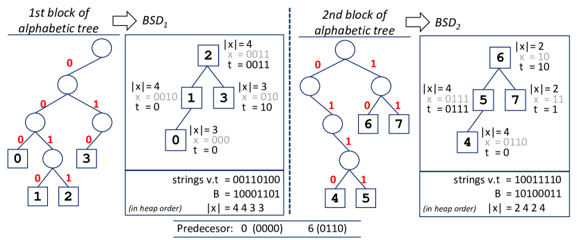
Figure 5: Our representation of the code for wavelet matrices of Figure 4. For each BSD structure we only store the concatenated strings $v.t$, their bitmap $B$, and the code lengths $|x|$. The first codes of each BSD structure are stored in the predecessor structure on the bottom, padded to $L=4$ bits.

3.3 Faster operations

In order to reduce the time $\mathcal{O}\!\left({\min(\ell,\lg L)}\right)$ to $\mathcal{O}\!\left({\lg\ell}\right)$, we manage to encode and decode in constant time the codewords of length up to $L^{\prime}=L^{\epsilon/2}$, for some constant $\epsilon>0$. For the longer codewords, since $L^{\prime}<\ell\leq L$, it holds that $\lg\ell=\Theta(\lg L)$, and thus we already process them in time $\mathcal{O}\!\left({\lg\ell}\right)$.

For encoding, we store a bitmap $B[1..\sigma]$, so that $B[i]=1$ iff the length of the codeword of the $i$th source symbol is at most $L^{\prime}$. We also store a table $S[1..2^{L^{\prime}}]$ so that, if $B[i]=1$, then $S[rank(B,i)]$ stores the codeword of the $i$th source symbol (only $2^{L^{\prime}}$ source symbols can have codewords of length up to $L^{\prime}$). To encode $i$, we check $B[i]$. If $B[i]=1$, then we output the codeword $S[rank(B,i)]$ in constant time; otherwise we encode $i$ as in Theorem 1

For decoding, we build a table $A[0..2^{L^{\prime}}-1]$ where, for any $0\leq j<2^{L^{\prime}}$, if the binary representation of $j$ is prefixed by the codeword of the $i$th codeword, which is of length $\ell\leq L^{\prime}$, then $S[j]=(i,\ell)$. Instead, if no codeword prefixes $j$, then $S[j]=\perp$. We then read the next $L$ bits of the stream and extract the first $L^{\prime}$ of those $L$ bits in a number $j$. If $S[j]=(i,\ell)$, then we have decoded the symbol $i$ in constant time and advance in the stream by $\ell$ bits. Otherwise, we proceed with the $L$ bits we have read as in Theorem 1.

The encoding and decoding time is then always bounded by $\mathcal{O}\!\left({\lg\ell}\right)$, as explained. The space for $B$, $S$, and $A$ is $\mathcal{O}\!\left({\sigma+2^{L^{\prime}}(L^{\prime}+\lg\sigma)}\right)\subseteq\mathcal{O}\!\left({\sigma+2^{L^{\epsilon}}}\right)$ bits, because $L^{\prime}+\lg\sigma=\mathcal{O}\!\left({L}\right)$ and $\mathcal{O}\!\left({L2^{L^{\epsilon/2}}}\right)\subseteq 2^{L^{\epsilon}}$.

Corollary 2

Given a probability distribution over an alphabet of $\sigma$ symbols, we can build an optimal alphabetic prefix-free code and store it in $\mathcal{O}\!\left({\sigma\lg L+2^{L^{\epsilon}}}\right)$ bits, where $L$ is the maximum codeword length and $\epsilon$ is any positive constant, such that we can encode and decode any codeword of length $\ell$ in $\mathcal{O}\!\left({\lg\ell}\right)$ time. The result assumes a $w$-bit RAM computation model with $L=\mathcal{O}\!\left({w}\right)$.

4 Near-Optimal Alphabetic Codes

Our approach to storing a nearly optimal alphabetic code compactly has two parts: first, we show that we can build such a code so that the expected codeword length is $\left(1+\mathcal{O}\!\left({1/\sqrt{\lg\sigma}}\right)\right)^{2}=1+\mathcal{O}\!\left({1/\sqrt{\lg\sigma}}\right)$ times the optimal, the codewords tree $\mathcal{B}$ has height at most $\lg\sigma+\sqrt{\lg\sigma}+3$, and each subtree rooted at depth $\lceil\lg\sigma-\sqrt{\lg\sigma}\rceil$ is completely balanced. Then, we manage to store such a tree in $o(\sigma)$ bits so that encoding and decoding take $\mathcal{O}\!\left({1}\right)$ time.

4.1 Balancing the codewords tree

Evans and Kirkpatrick [26] showed how, given a binary tree on $\sigma$ leaves, we can build a new binary tree of height at most $\lceil\lg\sigma\rceil+1$ on the same leaves in the same left-to-right order, such that the depth of each leaf in the new tree is at most 1 greater than its depth in the original tree. We can use their result to restrict the maximum codeword length of an optimal alphabetic code, for an alphabet of $\sigma$ symbols, to be at most $\lg\sigma+\sqrt{\lg\sigma}+3$, while forcing its expected codeword length to increase by at most a factor of $1+\mathcal{O}\!\left({1/\sqrt{\lg\sigma}}\right)$. To do so, we build the tree $\mathcal{B}$ for an optimal alphabetic code and then rebuild, according to Evans and Kirkpatrick’s construction, each subtree rooted at depth $\lceil\sqrt{\lg\sigma}\rceil$. The resulting tree, $\mathcal{B}_{lim}$, has height at most $\lceil\sqrt{\lg\sigma}\rceil+\lceil\lg\sigma\rceil+1$ and any leaf whose depth increases was already at depth at least $\lceil\sqrt{\lg\sigma}\rceil$. Although there are better ways to build a tree $\mathcal{B}_{lim}$ with such a height limit [27, 28], our construction is sufficient to obtain an expected codeword length for $\mathcal{B}_{lim}$ that is $1+\mathcal{O}\!\left({1/\sqrt{\lg\sigma}}\right)$ times the optimal.

Further, let us take $\mathcal{B}_{lim}$ and completely balance each subtree rooted at depth $\lceil\lg\sigma-\sqrt{\lg\sigma}\rceil$. The height does not increase and any leaf whose depth increases was already at depth at least $\lceil\lg\sigma-\sqrt{\lg\sigma}\rceil$, so the expected codeword length increases by at most a factor of

$$\frac{\lceil\sqrt{\lg\sigma}\rceil+\lceil\lg\sigma\rceil+1}{\lceil\lg\sigma-\sqrt{\lg\sigma}\rceil}=1+\mathcal{O}\!\left({1/\sqrt{\lg\sigma}}\right)\,.$$

Let $\mathcal{B}_{bal}$ be the resulting tree. Since the expected codeword length of $\mathcal{B}_{lim}$ is in turn a factor of $1+\mathcal{O}\!\left({1/\sqrt{\lg\sigma}}\right)$ larger than that of $\mathcal{B}$, the expected codeword length of $\mathcal{B}_{bal}$ is also a factor of $\left(1+\mathcal{O}\!\left({1/\sqrt{\lg\sigma}}\right)\right)^{2}=1+\mathcal{O}\!\left({1/\sqrt{\lg\sigma}}\right)$ larger than the optimal. The tree $\mathcal{B}_{bal}$ then describes our suboptimal code.

4.2 Representing the balanced tree

To represent $\mathcal{B}_{bal}$, we store a bitmap $B[1..\sigma]$ in which $B[i]=1$ if and only if the $i$th left-to-right leaf is:

• of depth less than $\lceil\lg\sigma-\sqrt{\lg\sigma}\rceil$, or

• the leftmost leaf in a subtree rooted at depth $\lceil\lg\sigma-\sqrt{\lg\sigma}\rceil$.

Note that each $1$ of $B$ corresponds to a node of $\mathcal{B}_{bal}$ with depth at most $\lceil\lg\sigma-\sqrt{\lg\sigma}\rceil$. Since there are $m=\mathcal{O}\!\left({2^{\lg\sigma-\sqrt{\lg\sigma}}}\right)$ such nodes, $B$ can be represented in compressed form as described in Section 2.2, using $m\lg(\sigma/m)+\mathcal{O}\!\left({m+\sigma/\lg^{c}\sigma}\right)=\mathcal{O}\!\left({2^{\lg\sigma-\sqrt{\lg\sigma}}\lg\sigma+\sigma/\lg^{c}\sigma}\right)$ bits, supporting $rank$ and $select$ in time $\mathcal{O}\!\left({c}\right)$. For any constant $c$, the term $\mathcal{O}\!\left({2^{\lg\sigma-\sqrt{\lg\sigma}}\lg\sigma}\right)=\mathcal{O}\!\left({\sigma/2^{\sqrt{\lg\sigma}-\lg\lg\sigma}}\right)$ is dominated by the second component, $\mathcal{O}\!\left({\sigma/\lg^{c}\sigma}\right)$.

For encoding in constant time we store an array $S[1..2^{\lceil\lg\sigma-\sqrt{\lg\sigma}\rceil}]$, which explicitly stores the codewords assigned to the leaves of $\mathcal{B}_{bal}$ where $B[i]=1$, in the same order of $B$. That is, if $B[i]=1$, then the code assigned to the symbol $i$ is stored at $S[rank(B,i)]$. Since the codewords are of length at most $\lceil\sqrt{\lg\sigma}\rceil+\lceil\lg\sigma\rceil+1=\mathcal{O}\!\left({\lg\sigma}\right)$, $S$ requires $\mathcal{O}\!\left({2^{\lg\sigma-\sqrt{\lg\sigma}}\lg\sigma}\right)=o(\sigma/\lg^{c}\sigma)$ bits of space, for any constant $c$. We can also store the length of the code within the same asymptotic space.

To encode the symbol $i$, we check whether $B[i]=1$ and, if so, we simply look up the codeword in $S$ as explained. If $B[i]=0$, we find the preceding 1 at $i^{\prime}=select(B,k)$ with $k=rank(B,i)$, which marks the leftmost leaf in the subtree rooted at depth $\lceil\lg\sigma-\sqrt{\lg\sigma}\rceil$ that contains the $i$th leaf in $\mathcal{B}$. Since the subtree is completely balanced, we can compute the code for the symbol $i$ in constant time from that of the symbol $i^{\prime}$: The balanced subtree has $r=i^{\prime\prime}-i^{\prime}$ leaves, where $i^{\prime\prime}=select(B,k+1)$, and its height is $h=\lceil\lg r\rceil$. Then the first $2r-2^{h}$ codewords are of the same length of the codeword for $i^{\prime}$, and the last $2^{h}-r$ have one bit less. Thus, if $i-i^{\prime}<2r-2^{h}$, the codeword for $i^{\prime}$ is $S[k]+i-i^{\prime}$, of the same length of that of $i$; otherwise it is one bit shorter, $(S[k]+2r-2^{h})/2+i-i^{\prime}-(2r-2^{h})=S[k]/2+i-i^{\prime}-(r-2^{h-1})$.

To be able to decode quickly, we store an array $A[0..2^{\lceil\lg\sigma-\sqrt{\lg\sigma}\rceil}-1]$ such that, if the $\lceil\lg\sigma-\sqrt{\lg\sigma}\rceil$-bit binary representation of $j$ is prefixed by the $i$th codeword, then $A[j]$ stores $i$ and the length of that codeword. If, instead, the $\lceil\lg\sigma-\sqrt{\lg\sigma}\rceil$-bit binary representation of $j$ is the path label to the root of a subtree of $\mathcal{B}_{bal}$ with size more than 1, then $A[j]$ stores the position $i^{\prime}$ in $B$ of the leftmost leaf in that subtree (thus $B[i^{\prime}]=1$). Again, $A$ takes $\mathcal{O}\!\left({2^{\lg\sigma-\sqrt{\lg\sigma}}\lg\sigma}\right)=o(\sigma/\lg^{c}\sigma)$ bits for any constant $c$.

Given a string prefixed by the $i$th codeword, we take the prefix of length $\lceil\lg\sigma-\sqrt{\lg\sigma}\rceil$ of that string (padding with 0s on the right if necessary), view it as the binary representation of a number $j$, and check $A[j]$. This either tells us immediately $i$ and the length of the $i$th codeword, or tells us the position $i^{\prime}$ in $B$ of the leftmost leaf in the subtree containing the desired leaf. In the latter case, since the subtree is completely balanced, we can compute $i$ in constant time: We find $i^{\prime\prime}$, $r$, and $h$ as done for encoding. We then take the first $\lceil\lg\sigma-\sqrt{\lg\sigma}\rceil+h$ bits of the string (including the prefix we had already read, and padding with a 0 if necessary), and interpret it as the number $j^{\prime}$. Then, if $d=j^{\prime}-S[rank(B,i^{\prime})]<2r-2^{h}$, it holds $i=i^{\prime}+d$. Otherwise, the code is one bit shorter and the decoded symbol is $i=i^{\prime}+2r-2^{h}+\lfloor(d-(2r-2^{h}))/2\rfloor=i^{\prime}+r-2^{h-1}+\lfloor d/2\rfloor$.

Figure 6 shows an example, where we have balanced from level $1$ instead of level $2$ (which is what the formulas indicate) so that the tree of Figure 3 undergoes some change. The subtrees starting at the two children of the root are then balanced and made complete. The array $S$ gives the codeword of the first leaves of both subtrees and $A$ gives the position in bitmap $B$ of the codewords of the nodes rooting the balanced subtrees. To encode 2, since it is the 3rd symbol ($i=3$), we compute $k=rank(B,3)=1$, $i^{\prime}=select(B,1)=1$, $i^{\prime\prime}=select(B,1+1)=7$, and $S[1]=0000$. The complete subtree then has $r=i^{\prime\prime}-i^{\prime}=6$ leaves and its height is $r=\lceil\lg 6\rceil=3$. The first $2r-2^{h}=4$ leaves are of depth $4$ like $S[1]$, and the other $2^{h}-r=2$ are of depth $3$. Since $i-i^{\prime}=2<4$, our codeword is of length $4$ and is computed as $S[1]+i-i^{\prime}=0010$. Instead, to decode $010$, we truncate it to length $1$, obtaining $j=0$. Since $A[0]=1$, the code is in the subtree that starts at $i^{\prime}=1$ in $B$. We compute $i^{\prime\prime}=7$, $r=6$, and $h=3$ as before. The first $1+h=4$ bits of our code is $j^{\prime}=0100$, which we had to pad with a $0$. Since $d=j^{\prime}-S[rank(B,1)]=0100-0000=4\geq 2r-2^{h}$, the code is of length $3$ and the source symbol is $i=1+6-2^{2}+2=5$, that is, 4.

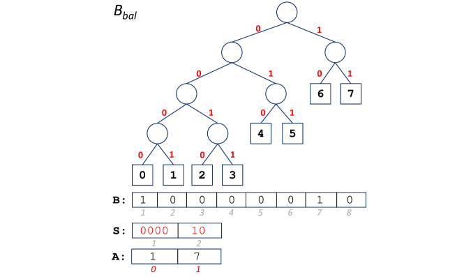
Figure 6: The alphabetic tree of Figure 3 balanced from level $1$. The resulting compressed sequence length is now $67$ bits (larger than a plain code, in this toy example).

Theorem 3

Given a probability distribution over an alphabet of $\sigma$ symbols, we can build an alphabetic prefix-free code whose expected codeword length is at most a factor of $1+\mathcal{O}\!\left({1/\sqrt{\lg\sigma}}\right)$ more than optimal and store it in $\mathcal{O}\!\left({\sigma/\lg^{c}\sigma}\right)$ bits, for any constant $c$, such that we can encode and decode any symbol in constant time $\mathcal{O}\!\left({c}\right)$.

5 Efficient Codes for Wavelet Matrices

We now show how to efficiently represent the prefix-free codes for wavelet matrices; recall Section 2.6. We first describe a representation based on the wavelet trees of Section 2.2. This is then used to design a space-efficient version that encodes and decodes codewords of length $\ell$ in time $\mathcal{O}\!\left({\ell}\right)$, and then a larger one that encodes and decodes in constant time.

5.1 Using wavelet trees

Given a code for wavelet matrices, we reassign the codewords of the same length such that the lexicographic order of the reversed codewords of that length is the same as that of their symbols. This preserves the property that the codewords of some length are numerically smaller than the corresponding prefixes of longer codewords in the lexicographic order of their reverses. The positive aspect of this reassignment is that all the information on the code can be represented in $\sigma\lg L$ bits as a sequence $D=d_{1},\ldots,d_{\sigma}$, where $d_{i}$ is the depth of the leaf encoding symbol $i$ in the codewords tree $\mathcal{B}$. We can represent $D$ with a wavelet tree using $\sigma\lg L\,(1+o(1))+\mathcal{O}\!\left({L\lg\sigma}\right)\subseteq\mathcal{O}\!\left({\sigma\lg L}\right)$ bits (Section 2.2), and then:

• $access(D,i)$ is the length $\ell$ of the codeword of symbol $i$;

• $rank_{\ell}(D,i)$ is the position (in reverse lexicographic order) of the leaf representing symbol $i$ among those of codeword length $\ell$; and

• $select_{\ell}(D,r)$ is the symbol corresponding to the $r$th codeword of length $\ell$ (in reverse lexicographic order).

Those operations take time $\mathcal{O}\!\left({1+\lg L/\lg w}\right)$, because the alphabet of $D$ is $\{1,\ldots,L\}$. Since we assume $L=\mathcal{O}\!\left({w}\right)$ (Section 2.1), this time is $\mathcal{O}\!\left({1}\right)$.

We are left with two subproblems. For decoding the first symbol encoded in a binary string, we need to find the length $\ell$ of its codeword and the lexicographic rank $r$ of its reverse among the reversed codewords of that length. With that information we have that the source symbol is $select_{\ell}(D,r)$. For encoding a symbol $i$, instead, we find the length $\ell=D[i]$ of its codeword and the lexicographic rank $r=rank_{\ell}(D,i)$ of its reverse among the reversed codewords of length $\ell$. Then we must find the codeword given $\ell$ and $r$.

We first present a solution that takes $\mathcal{O}\!\left({L\lg\sigma}\right)\subseteq\mathcal{O}\!\left({\sigma\lg L}\right)$ further bits and works in $\mathcal{O}\!\left({\ell}\right)$ time. We then present a solution that takes $\mathcal{O}\!\left({2^{\epsilon L}}\right)$ further bits, for any constant $\epsilon>0$, and works in less time.

5.2 A space-efficient representation

For each depth $d$ between 0 and $L$, let $\mathsf{nodes}(d)$ be the total number of nodes at depth $d$ in $\mathcal{B}$ and let $\mathsf{leaves}(d)$ be the number of leaves at depth $d$. Let $v$ be a node other than the root, let $u$ be $v$’s parent, let $r_{v}$ be the lexicographic rank (counting from 1) of $v$’s reversed path label among all the reversed path labels of nodes at $v$’s depth, and let $r_{u}$ be defined analogously for $u$. Then note the following facts:

1. Because $\mathcal{B}$ is optimal, every internal node has two children, so half the non-root nodes are left children and half are right children.

2. Because the reversed path labels of the left children at any depth start with a $0$, they are all lexicographically less than the reversed path labels of all the right children at the same depth, which start with a $1$.

3. Because of the ordering properties of these codes, the reversed path labels of all the leaves at any depth are lexicographically less than the reversed path labels of all the internal nodes at that depth.

It then follows that:

• $v$ is a leaf if and only if $r_{v}\leq\mathsf{leaves}(0pt(v))$;

• $v$ is $u$’s left child if and only if $r_{v}\leq\mathsf{nodes}(0pt(v))/2$;

• if $v$ is $u$’s left child then $r_{v}=r_{u}-\mathsf{leaves}(0pt(u))$; and

• if $v$ is $u$’s right child then $r_{v}=r_{u}-\mathsf{leaves}(0pt(u))+\mathsf{nodes}(0pt(v))/2$.

Of course, by rearranging terms we can also compute $r_{u}$ in terms of $r_{v}$.

We store $\mathsf{nodes}(d)$ and $\mathsf{leaves}(d)$ for $d$ between 0 and $L$, which requires $\mathcal{O}\!\left({L\lg\sigma}\right)$ bits. With the formulas above, we can decode the first codeword, of length $\ell$, from a binary string as follows: We start at the root $u$, $r_{u}=1$, and descend in $\mathcal{B}$ until we reach the leaf $v$ whose path label is that codeword, and return its depth $\ell$ and the lexicographic rank $r=r_{v}$ of its reverse path label among all the reversed path labels of nodes at that depth. We then compute $i$ from $\ell$ and $r$ as described with the wavelet tree. Note that these nodes $v$ are conceptual: we do not represent the nodes explicitly, but we still can compute $r_{v}$ as we descend left or right; we also know when we have reached a conceptual leaf.

For encoding $i$, we obtain as explained, with the wavelet tree, its length $\ell$ and the rank $r=r_{v}$ of its reversed codeword among the reversed codewords of that length. Then we use the formulas to walk up towards the root, finding in each step the rank $r_{u}$ of the parent $u$ of $v$, and determining if $v$ is a left or right child of $u$. This yields the $\ell$ bits of the codeword of $i$ in reverse order (0 when $v$ is a left child of $u$ and 1 otherwise), in overall time $\mathcal{O}\!\left({\ell}\right)$. This completes our first solution, which we evaluate experimentally in Section 6.

Theorem 4

Consider an optimal prefix-free code in which all the codewords of length $\ell$ come before the prefixes of length $\ell$ of longer codewords in the lexicographic order of the reversed binary strings. We can store such a code in $\sigma\lg L\,(1+o(1))+\mathcal{O}\!\left({L\lg\sigma}\right)\subseteq\mathcal{O}\!\left({\sigma\lg L}\right)$ bits — possibly after swapping symbols’ codewords of the same length — where $\sigma$ is the alphabet size and $L$ is the maximum codeword length, so that we can encode and decode any codeword of length $\ell$ in $\mathcal{O}\!\left({\ell}\right)$ time. The result assumes a $w$-bit RAM computation model with $L=\mathcal{O}\!\left({w}\right)$.

Figure 7 shows our representation for the codewords tree of Figure 4. To decode $110...$, we start at the root with $r_{0}=1$. The next bit to decode is a $1$, so we must go right: the node of depth $1$ is then $r_{1}=r_{0}-\mathsf{leaves}(0)+\mathsf{nodes}(1)/2=2$. The next bit to decode is again a $1$, so we go right again: the node of depth $2$ is $r_{2}=r_{1}-\mathsf{leaves}(1)+\mathsf{nodes}(2)/2=4$. The last bit to decode is a $0$, so we go left: the node of depth $3$ is $r_{3}=r_{2}-\mathsf{leaves}(2)=2$. Now we are at a leaf (because $r_{3}\leq\mathsf{leaves}(3)=2$) whose depth is $\ell=3$ and its rank is $r=r_{3}=2$. The corresponding symbol is then $select_{3}(D,2)=8$, that is, symbol 7. Instead, to encode 3, the symbol number $i=4$, we compute its codeword length $\ell=D[4]=3$ and its rank $r=rank_{3}(D,4)=1$. Our leaf then corresponds to $r_{3}=1$, and we discover the code in reverse order by waking upwards to the root. Since $r_{3}\leq\mathsf{nodes}(3)/2=2$, we are a left child (so the codeword ends with a $0$) and our parent has $r_{2}=r_{3}+\mathsf{leaves}(2)=3$. Since $r_{2}>\mathsf{nodes}(2)/2=2$, this node is a right child (so the codeword ends with $10$) and its parent has $r_{1}=r_{2}+\mathsf{leaves}(1)-\mathsf{nodes}(2)/2=1$. Finally, the new node is a left child because $r_{1}\leq\mathsf{nodes}(1)/2=1$, and therefore the codeword is $010$.

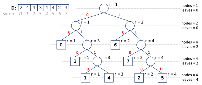
Figure 7: Our representation for the tree of Figure 4. We only store the sequence $D$ and the values $\mathsf{nodes}$ and $\mathsf{leaves}$ at each level. For each node $v$ we show its $r_{v}$ value.

Figure 8 shows another example with a sequence producing a less regular tree. Consider decoding $1110...$. We start at the root with $r_{0}=1$. The first bit to decode is a $1$, so we go right and obtain $r_{1}=r_{0}-\mathsf{leaves}(0)+\mathsf{nodes}(1)/2=2$. The next bit is also a $1$, so we go right again and get $r_{2}=r_{1}-\mathsf{leaves}(1)+\mathsf{nodes}(2)/2=4$. The third bit to decode is also a $1$, so we go right again to get $r_{3}=r_{2}-\mathsf{leaves}(2)+\mathsf{nodes}(3)/2=6$ (that is, the $4$th node of level $2$, minus the leaf with code $00$, shifted by all the $6/3$ nodes of level $3$ that descend by a $0$ and thus precede our node). Finally, the next bit is a $0$, so we go left, to node $r_{4}=r_{3}-\mathsf{leaves}(3)=1$ (that is, the $6$th node of level $3$ minus the $5$ leaves of that level). Now we are at a leaf because $r_{4}\leq\mathsf{leaves}(4)=2$. We leave to the reader finding the corresponding symbol 5 in $D$, as done for the previous example, as well as working out the decoding of the same symbol.

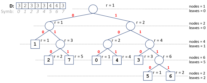
Figure 8: The representation of a less regular code, with the same notation of Figure 7, produced for the sequence “$14765232100214171$”.

5.3 Faster and larger

We now show how to speed up the preceding procedure so that we can perform $t$ steps on the tree in constant time, for some given $t$. From the formulas that relate $r_{u}$ and $r_{v}$ it is apparent that, given a node $u$ and the following $t$ bits to decode, the node $x$ we will arrive at depends only on the $\mathsf{nodes}$ and $\mathsf{leaves}$ values at the depths $0pt(u),\ldots,0pt(u)+t$. More precisely, the value $r_{x}$ is $r_{u}$ plus a number that depends only on the involved depths and the $t$ bits of the codeword to decode. Similarly, given $r_{x}$, the last $t$ bits leading to it, and the rank $r_{u}$ of the ancestor $u$ of $x$ at distance $t$, depend on the same values of $\mathsf{nodes}$ and $\mathsf{leaves}$.

Let us first consider encoding a source symbol. We obtain its codeword length $\ell$ and rank $r$ from the wavelet tree, and then extract the codeword. Consider all the path labels of a particular length that end with a particular suffix of length $t$: the lexicographic ranks of their reverses are consecutive, forming an interval. We can then partition the nodes at any depth $d$ by those intervals of rank values.

Let $x$ be a node at depth $d$, $u$ be its ancestor at distance $t$, and $r_{x}$ and $r_{u}$ be the rank values of $x$ and $u$, respectively. As per the previous paragraph, the partition interval where $r_{x}$ lies determines the last $t$ bits of $x$’s path label, and it also determines the difference between $r_{x}$ and $r_{u}$. For example, in level $d=3$ of Figure 8 and taking $t=2$, the codes of the nodes $x$ with rank $r=[1,1]$ end with $00$, those with ranks $r=[2,3]$ end with $10$, those with ranks $[4,4]$ end with $01$, and those with ranks $r=[5,6]$ end with $11$. The differences $r_{u}-r_{x}$ are $+1$ for the termination $00$, $-1$ for $10$, $-2$ for $01$, and $-4$ for $11$, the same for all the ranks in the same intervals.

We can then compute the codeword of length $\ell$ in $\mathcal{O}\!\left({\ell/t}\right)$ chunks of $t$ bits each, by starting at depth $d=\ell$ and using the formulas to climb by $t$ steps at a time until reaching the root (the last chunk may have less than $t$ bits).

For each depth $d$ having $s$ nodes, we store a bitmap $B_{d}[1..s]$, where $B_{d}[r]=1$ if $r$ is the first rank of the interval that ends with the same $t$ bits (or the same $d$ bits if $d<t$). A table $A_{d}[rank(B_{d},r)]$ then stores those $t$ bits and the difference that must be added to each $r_{x}$ in that interval to make it $r_{u}$. Across all the depths, the bitmaps $B_{d}$ add up to $\mathcal{O}\!\left({\sigma}\right)$ bits because $\mathcal{B}$ has $\mathcal{O}\!\left({\sigma}\right)$ nodes. Further, there are at most $2^{t}$ partitions in each depth, so the tables $A_{d}$ add up to $L\cdot 2^{t}$ entries, each using $\mathcal{O}\!\left({t+\lg\sigma}\right)$ bits: $t$ bits of the chunk and $1+\lg\sigma$ bits to encode $r_{u}-r_{x}$, since ranks are at most $\sigma$. In total, we use $\mathcal{O}\!\left({\sigma+L\,2^{t}(t+\lg\sigma)}\right)$ bits, which setting $t=\epsilon L/2$, for any constant $\epsilon>0$, is $\mathcal{O}\!\left({\sigma+2^{\epsilon L}}\right)$ because $t+\lg\sigma=\mathcal{O}\!\left({L}\right)$ and $L^{2}=\mathcal{O}\!\left({2^{\epsilon L/2}}\right)$. We can then encode any symbol in time $\mathcal{O}\!\left({L/t}\right)=\mathcal{O}\!\left({1/\epsilon}\right)$, that is, a constant.

For decoding we store a table that stores, for every depth $d$ that is a multiple of $t$, and every sequence $j$ of $t$ bits, a cell $(d,j)$ with the value to be added to $r_{u}$ in order to become $r_{x}$, where $u$ is any node at depth $0pt(u)=d$ and $x$ is the node we reach from $u$ if we descend using the $t$ bits of $j$. This table then has $(L/t)\cdot 2^{t}$ entries, each using $\mathcal{O}\!\left({\lg\sigma}\right)$ bits to encode the value to be added. With $t=\epsilon L/2$, the space is $\mathcal{O}\!\left({2^{\epsilon L}}\right)$ bits and we arrive at the desired leaf after $\mathcal{O}\!\left({1/\epsilon}\right)$ steps (note that our formulas allow us identifying leaves). Once we arrive at a leaf at depth $d$, we know the codeword length $\ell=d$ and the rank $r=r_{x}$, so we use the wavelet tree to compute the source symbol in constant time.

The obvious problem with this scheme is that it only works if the length $\ell$ of the codeword we find is a multiple of $t$. Otherwise, in the last step we will try to advance by $t$ bits when the leaf is at less distance. In this case our computation of $r_{x}$ will give an incorrect result.

Note from our formulas that the nodes $x$ at depth $d+k$ with $r_{x}\leq\mathsf{leaves}(d+k)$ are leaves and the others are internal nodes. Let $u$ be any node at depth $0pt(u)=d$ and $j$ be the bits of a potential path of length $t$ descending from $u$. If $x$ descends from $u$ by the sequence $j_{k}$ of the first $k$ bits of $j$, then the difference $g_{d,j}(k)=r_{x}-r_{u}$ depends only on $d$, $j$, and $k$ (indeed, our table stores precisely $g_{d,j}(t)$ at cell $(d,j)$). Therefore, the nodes $u$ that become leaves at depth $d+k$ are those with $r_{u}\leq\mathsf{leaves}(d+k)-g_{d,j}(k)$. We can then descend from node $u$ by a path with $s$ bits $j_{s}$ iff $r_{u}>m_{d,j}(s)$, with

$$m_{d,j}(s)~{}=~{}\max_{0\leq k<s}~{}\{\mathsf{leaves}(d+k)-g_{d,j}(k)\}.$$

We then extend our tables in the following way. For every cell $(d,j)$ we now store $t$ values $m_{d,j}(s)$, with $s=1,\ldots,t$, and the associated values $g_{d,j}(s)$. Note that $m_{d,j}(s)\leq m_{d,j}(s+1)$, so this sequence is nondecreasing. We make it strictly increasing by removing the smaller $s$ values upon ties. To find out how much we can descend from an internal node $u$ at depth $d$ by the $t$ bits $j$, we find $s$ such that $m_{d,j}(s)<r_{u}\leq m_{d,j}(s+1)$, and then we can descend by $s$ steps (and by $t$ steps if $r_{u}>m_{d,j}(t)$). To descend by $s$ steps to the descendant node $x$, we compute $r_{x}=r_{u}+g_{d,j}(s)$.

We find $s$ with a predecessor search on the $t$ values $m_{d,j}(s)$. One of the predecessor algorithms surveyed in Section 2.2 runs in time $\mathcal{O}\!\left({\lg_{w}t}\right)$, which is constant in the RAM model with $L=\mathcal{O}\!\left({w}\right)$ because $t=\epsilon L/2$. Therefore, the encoding time is still $\mathcal{O}\!\left({1/\epsilon}\right)$. The space is now multiplied by $t$ because the values $m_{d,j}$ and $g_{d,j}$ also fit in $\mathcal{O}\!\left({\lg\sigma}\right)$ bits, and thus it is still $\mathcal{O}\!\left({L2^{\epsilon L/2}}\right)\subseteq\mathcal{O}\!\left({2^{\epsilon L}}\right)$ bits.

Theorem 5

Consider an optimal prefix-free code in which all the codewords of length $\ell$ come before the prefixes of length $\ell$ of longer codewords in the lexicographic order of the reversed binary strings. We can store such a code in $\mathcal{O}\!\left({\sigma\lg L+2^{\epsilon L}}\right)$ bits — possibly after swapping symbols’ codewords of the same length — where $\sigma$ is the alphabet size, $L$ is the maximum codeword length, and $\epsilon>0$ is any positive constant, so that we can encode and decode any codeword in constant time. The result assumes a $w$-bit RAM computation model with $L=\mathcal{O}\!\left({w}\right)$.

6 Experiments

We have run experiments to compare the solution of Theorem 4 (referred to as WMM in the sequel, for Wavelet Matrix Model) with the only previous encoding, that is, the one used by Claude et al. [15] (denoted TABLE). Note that our codes are not canonical, so other solutions [9] do not apply.

Claude et al. [15] use for encoding a single table of $\sigma L$ bits storing the code of each symbol, and thus they easily encode in constant time. For decoding, they have tables separated by codeword length $\ell$. In each such table, they store the codewords of that length and the associated symbol, sorted by codeword. This requires $\sigma(L+\lg\sigma)$ further bits, and permits decoding by binary searching the codeword found in the wavelet matrix. Since there are at most $2^{\ell}$ codewords of length $\ell$, the binary search takes time $\mathcal{O}\!\left({\ell}\right)$.

For the sequence $D$ used in our WMM, we use binary Huffman-shaped wavelet trees with plain bitmaps (i.e., not compressed). The structures for supporting $rank$/$select$ require $37.5$% extra space, so the total space is $1.37\,\sigma\mathcal{H}_{0}(D)$, where $\mathcal{H}_{0}(D)\leq\lg L$ is the per-symbol zero-order entropy of the sequence $D$. We also add a small index to speed up select queries [29] (at decoding), which is parameterized with a sampling value that we set to $\{16,32,64,128\}$. Finally, we store the values $\mathsf{leaves}$ and $\mathsf{nodes}$, which add an insignificant $L\lg\sigma$ bits in total.

We used a prefix of three datasets in http://lbd.udc.es/research/ECRPC. The first one, EsWiki, contains a sequence of word identifiers generated by using the Snowball algorithm to apply stemming to the Spanish Wikipedia. The second one, EsInv, contains a concatenation of differentially encoded inverted lists extracted from a random sample of the Spanish Wikipedia. The third dataset, Indo was created with the concatenation of the adjacency lists of Web graph Indochina-2004, from http://law.di.unimi.it/datasets.php.

Table 1 provides some statistics about the datasets, starting with the number of symbols in the sequence ($n$) and the alphabet size ($\sigma$). $\mathcal{H}(P)$ is the entropy, in bits per symbol, of the frequency distribution $P$ observed in the sequence. This is close to the average length $\ell$ of encoded and decoded codewords. The last columns show the maximum codeword length $L$ and the zero-order entropy of the sequence $D$, $\mathcal{H}_{0}(D)$, in bits per symbol. This is a good approximation to the per-symbol size of our wavelet tree for $D$.

Collection	Length	Alphabet	Entropy	max code	Entropy of level
	($n$)	size ($\sigma$)	($\mathcal{H}(P)$)	length($L$)	entries ($\mathcal{H}_{0}(D)$)
EsWiki	200,000,000	1,634,145	11.12	28	2.24
EsInv	300,000,000	1,005,702	5.88	28	2.60
Indo	120,000,000	3,715,187	16.29	27	2.51

Table 1: Main statistics of the texts used.

Our test machine has an Intel(R) Core(tm) i7-3820@3.60GHz CPU (4 cores/8 siblings) and 64GB of DDR3 RAM. It runs Ubuntu Linux 12.04 (Kernel 3.2.0-99-generic). The compiler used was g++ version 4.6.4 and we set compiler optimization flags to -O9. All our experiments run in a single core and time measures refer to CPU user-time. The data to be compressed is streamed from the local disk and also output to disk using the regular buffering mechanism from the OS.

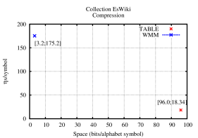
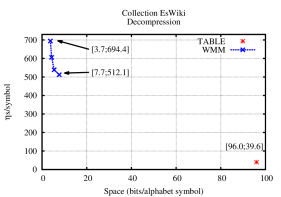
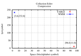
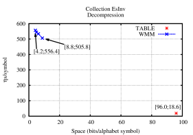
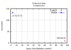
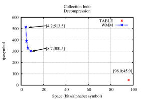
Figure 9: Size of code representations versus compression time (left) and decompression time (right). Time is measured in nanoseconds per symbol.

Figure 9 compares the space required by both code representations and their compression and decompression times. As expected, the space per symbol of our new code representation, WMM, is close to $1.37\,\mathcal{H}_{0}(D)$, whereas that of TABLE is close to $2L+\lg\sigma$. This explains the large difference in space between both representations, a factor of 23–30 times. For decoding we show the effect of adding the structure that speeds up select queries.

The price of our representation is the encoding and decoding time. While the TABLE approach encodes using a single table access, in 9–18 nanoseconds, our representation needs 130–230, which is 10–21 times slower. For decoding, the binary search performed by TABLE takes 20–45 nanoseconds, whereas our WMM representation requires 500–700 in the slowest and smallest variant (i.e., 11–30 times slower). Our faster variants require 300–500 nanoseconds, which is still 6.5–27 times slower.

7 Conclusions

A classical prefix-free code representation uses $\mathcal{O}\!\left({\sigma L}\right)$ bits, where $\sigma$ is the source alphabet size and $L$ the maximum codeword length, and encodes in constant time and decodes a codeword of length $\ell$ in time $\mathcal{O}\!\left({\ell}\right)$. Canonical prefix codes can be represented in $\mathcal{O}\!\left({\sigma\lg L}\right)$ bits, so that one can encode and decode in constant time. In this paper we have considered two families of codes that cannot be put in canonical form. Alphabetic codes can be represented in $\mathcal{O}\!\left({\sigma}\right)$ bits, but encoding and decoding takes time $\mathcal{O}\!\left({\ell}\right)$. We showed how to store an optimal alphabetic code in $\mathcal{O}\!\left({\sigma\lg L}\right)$ bits such that encoding and decoding any codeword of length $\ell$ takes $\mathcal{O}\!\left({\min(\ell,\lg L)}\right)$ time. We also showed how to store it in $\mathcal{O}\!\left({\sigma\lg L+2^{L^{\epsilon}}}\right)$ bits, where $\epsilon$ is any positive constant, such that encoding and decoding any such codeword takes $\mathcal{O}\!\left({\lg\ell}\right)$ time. We thus answered an open problem from the conference version of this paper [1]. We then gave an approximation that worsens the average code length by a factor of $1+\mathcal{O}\!\left({1/\sqrt{\lg\sigma}}\right)$, but in exchange requires only $o(\sigma)$ bits and encodes and decodes in constant time.

We then consider a family of codes where, at any level, the strings leading to leaves lexicographically precede the strings leading to internal nodes, if we read them upwards. For those we obtain a representation using $\mathcal{O}\!\left({\sigma\lg L}\right)$ bits and encoding and decoding in time $\mathcal{O}\!\left({\ell}\right)$, and even in constant time if we use $\mathcal{O}\!\left({2^{\epsilon L}}\right)$ further bits, where $\epsilon$ is again any positive constant. We have implemented the simple version of these codes, which are used for compressing wavelet matrices [15], and shown that our encodings are significantly smaller than classical ones in practice (up to 30 times), albeit also slower (up to 30 times). We note that in situations when our encodings are small enough to fit in a faster level of the memory hierarchy, they are likely to be also significantly faster than classical ones.

We leave as an open question extending our results to dynamic coding [30, 31, 32, 33, 34] and to codes with unequal codeword-symbol costs [32, 35].

References

- [1] A. Fariña, T. Gagie, G. Manzini, G. Navarro, A. Ordóñez, Efficient and compact representations of some non-canonical prefix-free codes, in: Proc. 23rd International Symposium on String Processing and Information Retrieval (SPIRE), 2016, pp. 50–60.
- [2] T. Cover, J. Thomas, Elements of Information Theory, 2nd Edition, Wiley, 2006.
- [3] D. A. Huffman, A method for the construction of minimum-redundancy codes, Proceedings of the Institute of Electrical and Radio Engineers 40 (9) (1952) 1098–1101.
- [4] A. Moffat, Word-based text compression, Software Practice and Experience 19 (2) (1989) 185–198.
- [5] N. Ziviani, E. Moura, G. Navarro, R. Baeza-Yates, Compression: A key for next-generation text retrieval systems, IEEE Computer 33 (11) (2000) 37–44.
- [6] P. Ferragina, R. Giancarlo, G. Manzini, M. Sciortino, Boosting textual compression in optimal linear time, Journal of the ACM 52 (4) (2005) 688–713.
- [7] N. R. Brisaboa, A. Fariña, G. Navarro, J. Paramá, Lightweight natural language text compression, Information Retrieval 10 (2007) 1–33.
- [8] E. S. Schwartz, B. Kallick, Generating a canonical prefix encoding, Communications of the ACM 7 (1964) 166–169.
- [9] T. Gagie, G. Navarro, Y. Nekrich, A. Ordóñez, Efficient and compact representations of prefix codes, IEEE Transactions on Information Theory 61 (9) (2015) 4999–5011.
- [10] N. Brisaboa, G. Navarro, A. Ordóñez, Smaller self-indexes for natural language, in: Proc. 19th International Symposium on String Processing and Information Retrieval (SPIRE), 2012, pp. 372–378.
- [11] M. A. Martínez-Prieto, N. Brisaboa, R. Cánovas, F. Claude, G. Navarro, Practical compressed string dictionaries, Information Systems 56 (2016) 73–108.
- [12] G. Navarro, Wavelet trees for all, Journal of Discrete Algorithms 25 (2014) 2–20.
- [13] T. C. Hu, A. C. Tucker, Optimal computer search trees and variable-length alphabetical codes, SIAM Journal of Applied Mathematics 21 (4) (1971) 514–532.
- [14] J. I. Munro, V. Raman, Succinct representation of balanced parentheses and static trees, SIAM Journal of Computing 31 (3) (2001) 762–776.
- [15] F. Claude, G. Navarro, A. Ordóñez, The wavelet matrix: An efficient wavelet tree for large alphabets, Information Systems 47 (2015) 15–32.
- [16] M. Pătraşcu, M. Thorup, Time-space trade-offs for predecessor search, in: Proc. 38th Annual ACM Symposium on Theory of Computing (STOC), 2006, pp. 232–240.
- [17] D. R. Clark, Compact PAT trees, Ph.D. thesis, University of Waterloo, Canada (1996).
- [18] J. I. Munro, Tables, in: Proc. 16th Conference on Foundations of Software Technology and Theoretical Computer Science (FSTTCS), 1996, pp. 37–42.
- [19] M. Pǎtraşcu, Succincter, in: Proc. 49th Annual IEEE Symposium on Foundations of Computer Science (FOCS), 2008, pp. 305–313.
- [20] R. Grossi, A. Gupta, J. S. Vitter, High-order entropy-compressed text indexes, in: Proc. 14th Annual ACM-SIAM Symposium on Discrete Algorithms (SODA), 2003, pp. 841–850.
- [21] D. Belazzougui, G. Navarro, Optimal lower and upper bounds for representing sequences, ACM Transactions on Algorithms 11 (4) (2015) article 31.
- [22] G. Navarro, Compact Data Structures – A practical approach, Cambridge University Press, 2016.
- [23] L. G. Kraft, A device for quantizing, grouping, and coding amplitude modulated pulses, M.Sc. thesis, EE Dept., MIT (1949).
- [24] A. Moffat, A. Turpin, On the implementation of minimum-redundancy prefix codes, IEEE Transactions on Communications 45 (10) (1997) 1200–1207.
- [25] A. Gupta, W.-K. Hon, R. Shan, J. S. Vitter, Compressed data structures: Dictionaries and data-aware measures, Theoretical Computer Science 387 (3) (2007) 313–331.
- [26] W. Evans, D. G. Kirkpatrick, Restructuring ordered binary trees, Journal of Algorithms 50 (2004) 168–193.
- [27] R. L. Wessner, Optimal alphabetic search trees with restricted maximal height, Information Processing Letters 4 (1976) 90–94.
- [28] A. Itai, Optimal alphabetic trees, SIAM Journal of Computing 5 (1976) 9–18.
- [29] G. Navarro, E. Providel, Fast, small, simple rank/select on bitmaps, in: Proc. 11th International Symposium on Experimental Algorithms (SEA), 2012, pp. 295–306.
- [30] T. Gagie, Dynamic Shannon coding, in: Proc. 12th Annual European Symposium on Algorithms (ESA), 2004, pp. 359–370.
- [31] T. Gagie, M. Karpinski, Y. Nekrich, Low-memory adaptive prefix coding, in: Proc. 19th Data Compression Conference (DCC), 2009, pp. 13–22.
- [32] T. Gagie, Y. Nekrich, Worst-case optimal adaptive prefix coding, in: Proc. 16th International Symposium on Algorithms and Data Structures (WADS), 2009, pp. 315–326.
- [33] T. Gagie, Y. Nekrich, Tight bounds for online stable sorting, Journal of Discrete Algorithms 9 (2) (2011) 176–181.
- [34] M. J. Golin, J. Iacono, S. Langerman, J. I. Munro, Y. Nekrich, Dynamic trees with almost-optimal access cost, in: Proc. 26th Annual European Symposium on Algorithms (ESA), 2018, pp. 38:1–38:14.
- [35] M. J. Golin, J. Li, More efficient algorithms and analyses for unequal letter cost prefix-free coding, IEEE Transactions on Information Theory 54 (8) (2008) 3412–3424.