Criteria for folding in structure-based models of proteins

Abstract

In structure-based models of proteins, one often assumes that folding is accomplished when all contacts are established. This assumption may frequently lead to a conceptual problem that folding takes place in a temperature region of very low thermodynamic stability, especially when the contact map used is too sparse. We consider six different structure-based models and show that allowing for a small, but model-dependent, percentage of the native contacts not being established boosts the folding temperature substantially while affecting the time scales of folding only in a minor way. We also compare other properties of the six models. We show that the choice of the description of the backbone stiffness has a substantial effect on the values of characteristic temperatures that relate both to equilibrium and kinetic properties. Models without any backbone stiffness (like the self-organized polymer) are found to perform similar to those with the stiffness, including in the studies of stretching.

I Introduction

Globular proteins that are found in nature are special sequences of amino acids that fold rapidly into their native states under physiological conditions Anfinsen ; ChanDill . The folding process in such proteins is considered to take place through motion in a mildly rugged free energy landscape with a prominent native basin Wolynes ; DillNat ; Nymeyer . Such a landscape forms through the principles of minimal frustration and maximal compatibility Bryngelson . On the other hand, random sequences are expected to form rough landscapes in which many local minima compete for occupancy, as illustrated in a model, for instance, in ref. Garstecki .

The question: what sequences make good folders, has been addressed mostly in the context of lattice models and various criteria have been proposed. One of these is that the lowest energy state – the native state – should have large thermodynamic stability Shakhnovich . Another is that the location of the specific-heat maximum should coincide with that of the structural susceptibility Camacho ; Klimov ; Folddes . It should be noted that the specific heat is a measure of fluctuations in the energy whereas the susceptibility is a measure of fluctuations in the number of pairs of ”amino acids” which stay at their native spatial separation. A more intuitional criterion has been proposed by Socci and Onuchic Socci . It is formulated in terms of two temperatures ($T$): $T_{f}$ and $T_{g}$. The former is the folding (or melting) temperature that depends on the energy spectrum and defines a temperature below which the probability of occupancy of the native state, $P_{0}$, is substantial. The latter relates to the dynamics and is the $T$ of the glass transition below which the protein gets trapped in a non-native state and folding times, $t_{f}$, become very long. Bad folders are then those sequences for which $T_{f}\;<\;T_{g}$. The larger the ratio of $T_{f}$ to $T_{g}$, the better the folding properties of the sequence.

The concepts behind this picture appear to be satisfactory in lattice models where the conformations, including the native one, are defined in a clear-cut manner and are structurally separated. Small lattice systems are simple enough to even allow for Master-equation based exact analysis of the folding process badgo . Here, we show that conceptual problems arise in off-lattice models and that they can be remedied by slightly relaxing the criteria for what it means for the system to stay in its native state. We focus on the highly studied structure-based, or Go-like, coarse-grained model Go ; Nymeyer ; Takada which, by its construction, leads to folding with a minimal obstruction. This model has various variants Karanicolas ; Paci0 ; Levy ; WestPaci ; models but, invariably, it is defined primarily in terms of the contact map which specifies which pairs of amino acids form a non-bonded interaction (most often through a hydrogen bond) in the native state, which itself may be taken from the Protein Data Bank (PDB) pdb . The contact maps can be used in all-atom simulations for descriptive purposes, but in the structure-based models they also define the dynamics of the system because the contacts are endowed with effective potentials. The minima of the potentials are located at the native separations.

In molecular dynamics studies of folding, one starts from an extended conformation and evolves the system until the native state is reached. Time $t_{f}$ corresponds to the median first passage time. In the simplest approach, the native state is declared to be reached when all of the native contacts become established. Similarly, $P_{0}$ is calculated as the probability of all contacts being established simultaneously in a long equilibrated run and $T_{f}$ corresponds to a $T$ at which $P_{0}$ crosses $\frac{1}{2}$. The plot of $t_{f}$ as a function of $T$ is typically U-shaped and the $T$ at the center of the U will be denoted as $T_{min}$. The corresponding optimal $t_{f}$ will be denoted as $t_{opt}$. We define $T_{g}$ operationally as the $T$ at which $t_{f}\;=\;3\;t_{opt}$ on the low-$T$ side of the U.

The puzzling observation is that with these simple definitions, $T_{min}$ in off-lattice models is often found in the region in which $P_{0}$ is very small – some previous examples are in refs. Hoang2 ; thermtit ; Jaskolski . Furthermore, there are many Go-model-based proteins for which the supposedly well folding chains are technically bad folders as they have a $T_{f}$ that is smaller or nearly equal to the corresponding value of $T_{g}$. Here, we examine 21 proteins within six Go-like models and find that a minor change in the definition of what it means to be in the native state makes $T_{f}$ to coincide with $T_{min}$ in all cases. The change involves requiring that a fraction, $p$, or more of the native contacts is established simultaneously, where $p$, instead of being equal to 1 as in the simple approach, is changed to $0.97\;\lesssim\;p\;<1$. The precise value of $p$ depends on the model and, to a lesser extent, on the protein. This result indicates that a situation with a few missing contacts makes the system practically reside within the very bottom of the native basin. We also find that the small reduction in $p$ leaves the $t_{f}$s nearly intact while boosting the apparent thermodynamic stability in a substantial manner. Relaxing the definition involved in calculating $P_{0}$ is expected to enhance the apparent stability. What is surprising, however, is that making the model system technically a good folder requires to shift $p$ away from 1 by only 3 percentage points or less.

It should be noted that the concept of the effective $P_{0}$, the fraction of time in which all contacts are made simultaneously, is quite distinct from that of the average fraction, $Q$, of the native contacts that are present. It is often assumed that the temperature $T_{Q}$ corresponding to crossing of $Q$ through $\frac{1}{2}$ signals a transition to folding. This assumption does not seem to have been tested by the actual determination of the corresponding $t_{f}$s. An argument in favor of this idea can be derived from the behavior of the $Q$-dependent free energy, $F(Q)$, which develops two minima which are of equal depths at a $T\approx T_{Q}$. However, at $Q$ of $\frac{1}{2}$, various subdomains may be set correctly without a proper establishment of the overall shape of the protein – and hence the relevance of $P_{0}$ instead of $Q$.

Furthermore, an exact analysis transition of a discretized $\beta$-hairpin, performed within the so called Munoz-Eaton model Eaton , indicates that $Q$ does not constitute a reaction coordinate even for such a simple system (see also refs. badgo ; Niewiecz ). This is related to the fact that Go-like models are defined in terms of contacts, but not in terms of $Q$. It should be noted, however, that all-atom simulations of a 3-helix bundle interpreted in terms of a Bayesian framework suggest that using $Q$ is a reasonable approximation in this case Bundle . In each of the models studied here, $T_{Q}$ is found to be close to the location of a maximum in the specific heat. The corresponding transition, however, should be associated with an onset of globular conformations since $T_{Q}$ is significantly higher than $T_{min}$ and well above the whole region of $T$s in which folding to one of the globular states – the native state – is appreciable. We find that at $T_{Q}$ the mean radius of gyration decreases rapidly on cooling. We also show that the $T$-range of proper folding and other characteristics, such as mechanostability, depend on the description of the backbone stiffness.

There are two ways of looking at the folding process. The perspective taken here is that it is a kinetic phenomenon. Another is that it is a smoothed out equilibrium phase transition that should be characterized through trajectories that last much longer than typical folding times. Studying $F(Q)$ is an approximate way to describe this transition. In this paper, we show that the two perspective can be made compatible if the equilibrium description is focused on $P_{0}$, i.e. on the fraction of time in which nearly all contacts are present instead of on average number of contacts. Fluctuations in the total energy do not indicate folding. There is some analogy to spin glasses here. Phase transitions in ferromagnets show, in the thermodynamic limit, as a divergence in the magnetic susceptibility, which is a measure of fluctuations in magnetization and is related to spin-spin correlation functions. However, in spin glasses, it is the nonlinear susceptibility Binder ; Hertz ; Gingras , and not susceptibility, that is sensitive to the transition from the paramagnetic phase. At the transition, the susceptibility displays merely a cusp. This nonlinear susceptibility is related to different spin correlations.

II Structure-based models studied

The six models we discuss here differ by the selection of the contact potential and the description of the local backbone stiffness, but the contact map is common: it is the map denoted by OV+rCSU in ref. Wolek , which is an extension of the OV map. The OV map is derived by considering overlaps between effective spheres assigned to heavy atoms in the native state. The radii are equal to the van der Waals radii multiplied by 1.24 Tsai . The rCSU part adds to OV those contacts which are identified by considerations of a chemical nature. In the case of the highly mechanostable I27 domain of titin (pdb:1TIT), the most important role of rCSU is to add an ionic bridge which contributes to the strength of a mechanical clamp in this protein. Generally, OV+rCSU leads to similar and sometimes superior folding properties compared to OV. The improvements show as the broader outline of the U-shaped dependence of $t_{f}$ on $T$ and stronger thermal stability. The potentials assigned to the contacts between residues $i$ and $j$ are given by

$$V(r_{ij})=\epsilon\;[(\frac{r_{ij}}{\sigma_{ij}})^{12}\;-\;(\frac{r_{ij}}{\sigma_{ij}})^{\lambda}]$$ (1)

where $\lambda$ is either 6 (the 12-6 potential) or 10 (the 12-10 potential). The parameters $\sigma_{ij}$ are derived pair-by-pair from the native distances between the residues – the minimum of the potential must coincide with the $\alpha$-C–$\alpha$-C distance. Consecutive $\alpha$-C atoms are tethered by the harmonic potential $k_{r}\;(r_{i,i+1}-r^{n}_{i,i+1})^{2}$, where $r^{n}_{i,i+1}$ is the native distance between $i$ and $i+1$. Note that the stiffness coefficient $k_{r}$ used here incorporates the customary factor of $\frac{1}{2}$ in the Hookean energy term. We shall adopt this convention in the definition of other harmonic terms discussed below.

We consider three versions of the local backbone stiffness. In many of our previous works JPCM ; plos , we have used the chirality (CH) potential $V^{CH}=\kappa\varepsilon\;\sum_{i=2}^{N-2}\;(C_{i}-C_{i}^{n})^{2}$ where $N$ is the number of residues and the coeffcient $\kappa$ is set to $\frac{1}{2}$, as $t_{f}$ ceases to be $\kappa$-dependent at larger values of $\kappa$ Kwiatek . The chirality of residue $i$ is defined as $C_{i}\;=\;(\vec{v}_{i-1}\times\vec{v}_{i})\cdot\vec{v}_{i+1}/d_{0}^{3}$ where $\vec{v}_{i}=\vec{r}_{i+1}-\vec{r}_{i}$ and $d_{0}$ is the average $r^{n}_{i,i+1}$. $C_{i}^{n}$ is the native value of $C_{i}$.

A more common way to account for the stiffness is to combine the bond-angle term $V_{\theta}=k_{\theta}\;(\theta-\theta_{n})^{2}$ with the dihedral term $V_{\phi}=K^{1}_{\phi}[1-cos(\phi-\phi_{n})]+K^{3}_{\phi}[1-cos(3(\phi-\phi_{n}))]$ where the subscript $n$ indicates the native values. For small departures of $\phi$ from $\phi_{n}$, $V_{\phi}=k_{\phi}\;(\phi-\phi_{0})^{2}$, where $k_{\phi}=\frac{1}{2}(K^{1}_{\phi}+9K^{3}_{\phi}$). In this limit, the dihedral term is equivalent to the chirality potential models . The values of the coefficients can be derived through all-atom simulations by matching average conformation-dependent energies to the coarse-grained expressions. Poma et al. Poma have studied sugar-protein complexes at room $T$s in this way and, as a byproduct, derived the following effective values for the parameters pertaining to proteins: $\epsilon$=1.5 kcal/mol, $k_{r}$=100 kcal/(mol Ų), $k_{\theta}$=45 kcal/(mol rad²), and $k_{\phi}$=5 kcal/(mol rad²). The contacts considered were defined by using the OV approach and the contact potential was 12-6. In units of $\epsilon$, these parameters are: $k_{r}$=66.66 $\epsilon$/Ų, $k_{\theta}$= 30 $\epsilon$/rad², and $k_{\phi}$= 3.33 $\epsilon$/rad². Assuming, for simplicity, the equality of the two dihedral coeffcients, we get $K^{1}_{\phi}=K^{3}_{\phi}$=0.66 $\epsilon$/rad². This model of the backbone stiffness will be denoted as AN (for angular). A similar set of values for the backbone stiffness has been used by Clementi et al. Clementi (with a different contact map). It is: $k_{r}$=100 $\epsilon$/Ų, $k_{\theta}$=20 $\epsilon$/rad², $K^{1}_{\phi}$=1 $\epsilon$/rad², and $K^{3}_{\phi}$=0.5 $\epsilon$/rad². This model will be denoted as AN’.

Finally, we consider models with no backbone stiffness at all, such as the self organized polymer (SOP) Hyeon ; Mickler . In the original SOP model, the harmonic representation of the peptide bond is expressed as a combination of the 12-6 and FENE potentials so that they act partially as the 12-6 contact energies to accelerate the numerics. Here, we use the SOP idea of not including any backbone stiffness also to the systems with the 12-10 contacts. We provide comparisons of protein stretching in the SOP models relative to the models with finite backbone stiffness. Note that the contact map in the original SOP model is defined through a cutoff distance whereas we use OV+rCSU.

The models we study here can be characterized by pairs of symbol such that the first symbol denotes the contact potential and the second – the model of the backbone stiffness. These are: I – (12-6, CH), II – (12-6, AN), III – (12-10, AN), IV – (12-10, AN’), V – (12-6, SOP), VI – (12-10, SOP). Each of these is studied as described in refs. Hoang2 ; JPCM ; plos using our own code. In particular, we use the overdamped Langevin thermostat and the characteristic time scale in the simulations, $\tau$, is of order 1 ns. The equations of motion were solved by the 5th order predictor-corrector method. Due to overdamping, our code is equivalent to the Brownian dynamics approach. A contact is considered to be established if its length is within 1.5 $\sigma$ or 1.2 $\sigma$ for the 12-6 and 12-10 potentials respectively JPCM ; Clementi .

The equilibrium parameters are determined on at least 3 long trajectories that last for 100 000 $\tau$.

It should be noted that the all-atom derived coarse-grained parameters generally depend on the location in the sequence and on the protein so they should be considered more as an order of magnitude estimates than precise values. In particular, the effective $\epsilon$ calculated within the $\beta$ sheets has been found to be $1.43\pm 0.3$ kcal/mol and within the $\alpha$ helices: $1.6\pm 0.9$ Poma . The uniform value of 1.5 kcal/mol used above has been selected for two reasons: 1) it is characteristic of the turn regions and 2) it coincides with the strength of a better-binding hydrogen bond. It corresponds to 755 K so the room temperature ought to be about 0.4$\epsilon/k_{B}$. However, due to the considerable uncertainty in this assessment, our previous practice has been to assume, when using models with a uniform $\epsilon$, that the room $T$ situation occurs when folding is optimal as this is when the model protein behaves as the real one. $\epsilon$ of 1.5 kcal/mol is consistent with 1.55 kcal/mol (or 106$\pm$ 16 pN Å, which itself is consistent with 110 pN Å of ref. plos ) that was obtained by matching characteristic values of the force $F_{max}$, needed to unravel proteins by constant-speed stretching within the coarse-grained model, to the experimental results Wolek . This estimate involves making extrapolations to the experimental speeds and adopting the OV-based contact map. When using the OV+rCSU map and 38 proteins the effective $\epsilon$ becomes 1.35 kcal/mol (or 93$\pm$14 pN Å) Wolek .

III Results

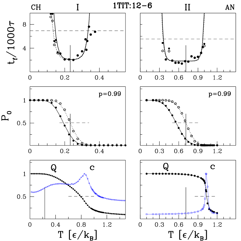
Figure 1: Kinetic and thermodynamic properties of models I (the left panels) and II (the right panels). The explanation of the symbols and lines used is provided in the main text. In the middle and bottom panels, the error bars are smaller than the size of the symbols. In the top panels, a measure of the uncertainty is given by the deviation of the data points from the fitting lines.

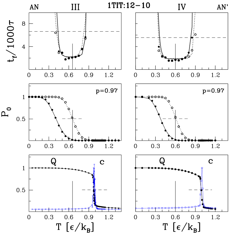
Figure 2: Similar to Figure 1 but for models III and IV.

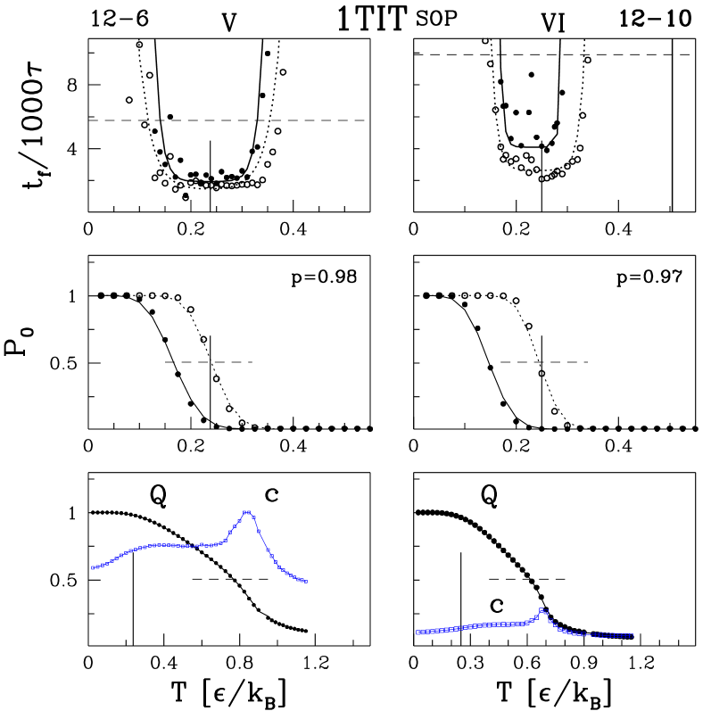
Figure 3: Similar to Figure 1 but for models V and VI.

The results pertaining to the thermodynamic and folding properties of the six models are illustrated in Figures 1, 2, and 3 for the I27 domain of titin. Mechanical stability of this protein has been assessed experimentally in many studies Rief ; titin ; Paci ; Oberhauser . The OVrCSU contact map for 1TIT consists of 198 contacts. Table I summarizes the results for all of the 21 proteins studied. The bottom panels show the $T$-dependence of $Q$ and $c$ – the specific heat normalized to its maximal value. These two quantities do not depend on the choice of $p$. The top panels show the median $t_{f}$s and the middle panels show the effective $P_{0}$. The general convention is that the solid data points connected by the solid lines correspond to $p$ of 1 (the undoctored value) whereas the open symbols connected by the dotted lines relate to the value of $p$ at which $T_{f}$ is in the very middle of the U-shaped folding curve – it is written in the right-hand corner of the middle panels. This value of $T_{f}$ is indicated by the vertical line. The folding curve is obtained by fitting the results based on at least 105 trajectories to the function described by $d_{1}\cosh(ax+b)+d_{2}$. The horizontal dashed lines indicate the level of the optimal $t_{f}$ multiplied by three from which an estimate of $T_{g}$ can be deduced. The horizontal lines in the middle and bottom panels indicate the level corresponding to $\frac{1}{2}$ (either for $P_{0}$ or for $Q$).

The shift in the apparent $T_{f}$ varies between 0.04 $\epsilon/k_{B}$ for model I and 0.25 $\epsilon/k_{B}$ for model III. It is 0.13, 0.22, 0.06, and 0.11 $\epsilon/k_{B}$ for models II, IV, V, and VI respectively. The 12-10 potentials are generally effectively more contained, or narrower, than the 12-6 ones and the effects of $p$ being smaller than 1 are stronger. Even the shifted effective values of $T_{f}$ are much lower by at least 50% than $T_{Q}$. On the other hand, the separation between $T_{Q}$ and $T_{max}$ does not exceed 0.07 $\epsilon/k_{B}$ in any model. The typical value of $T_{max}$ is of order 1 $\epsilon/k_{B}$ (though the smallest is 0.7 $\epsilon/k_{B}$ model VI and then it is 0.85 $\epsilon/k_{B}$ model I) which is puzzlingly high. The SOP model V has properties which are very similar to that of model I: the kinetics are close but at $p$=1 the stability of model I is higher. We find that when we remove the dihedral term in model II, while keeping the bond-angle term, $T_{min}$ shifts to a half-way position between models I and II.

We now consider the mechanical stability. Figure 4 illustrates stretching of 1TIT for $T=T_{min}$ and $T=T_{Q}$. The terminal residues of the protein are attached to two harmonic springs JPCM ; plos . One of the springs is anchored at one end and another is moving at a speed of 0.005 Å/$\tau$. We monitor the force, $F$, exerted by the protein on the moving spring as a function of the moving end displacement, $d$. In the initial state, the protein is set in its native state. When pulling is implemented at $T=T_{min}$, the $F-d$ patterns obtained by using the six models are seen to be remarkably similar though the heights of the force peaks are distinct. On the other hand, at $T_{Q}$, the force maxima are within the noise level. Notice that one cannot model experiments on stretching by simulating the corresponding kinetics at $T_{Q}$ (or $T_{max}$ which is very close to $T_{Q}$).

When comparing mechanostability of many proteins, as in ref.plos , it is convenient to choose one fixed $T$ that, for most proteins, would be within the basin of good foldability, though not necessarily equal to $T_{min}$. For models I, V, and VI such a temperature is 0.3 $\epsilon/k_{B}$. For 1TIT at this $T$, we get $<F_{max}>$ of 2.04$\pm$0.14, 2.05$\pm$0.12, and 2.44$\pm$0.09 $\epsilon$/Å respectively when extrapolating to the typical experimental speed of 600 nm/s titin . These estimates were obtained based on 100 trajectories. It should be noted, however, that each model has its own calibration of the value of $\epsilon$ Wolek . On considering 46 cases of the theory-experiment comparison (in addition to 38 of ref. Wolek , also 1QYS 1QYS , 2 directions of stretching for 1A1M 1A1M and 5 experimental pulling speeds for 1G6P (1G6P, )), we get the following calibrations for $\epsilon$: 93.1$\pm$15.1, 119.7$\pm$28.0 and 92.2$\pm$11.9 pN Å for models I, V, and VI respectively. The corresponding values of the coefficient of determination, $R^{2}$, are 0.846, 0.622 and 0.661, indicating that model I correlates with the experiment much better than the simpler SOP models. Similar estimates apply when stretching at the individually determined $T_{min}$.

In summary, the simple criterion of folding – that all contacts are established – may often lead to a perception that the structure-based model is unphysical because its thermodynamic stability is substantial in a low-temperature region in which folding is difficult or absent. This may happen especially when the contact map has too few elements to be appropriate dynamically, as is the case of, for instance, the CSU-based contact map Sobolev used in ref. Clementi . One needs to have a sufficient inter-residue connectivity for a model protein stay three-dimensional on its own Maxwell ; Thorpe ; Gomez . There are many definitions of the contact map and none of them is perfect. The OV+rCSU map selected here is particularly good, as tested in ref. Wolek but even this one does not remove the unphysicality. We have argued here, that allowing for a small percentage of the native contacts not being established boosts the $T_{f}$ substantially but affects the time scales of folding only in a minor way (with the exception of model VI). Determination of the effective thermodynamic stability should then be less strict (which also helps in hiding imperfections in the definition of the contact map) for the model to work well. The simple strict criterion, however, is simpler to use because it does not require having the knowledge of the exact value of the parameter $p$. It should be quite adequate when comparing relative thermodynamic stabilities of proteins. The good performance of the SOP models testifies to the fact that the properties of the structure-based models depends primarily on the contact map, though the particular choices for the backbone stiffness affect the optimal folding temperatures.

Model polypeptide chains can be used to describe globular proteins if folding takes place in the temperature range in which getting to the native state is associated with a substantial probability of staying in the vicinity of this state. We have introduced parameter $p$ that defines what should be meant by the effective native vicinity: the temperature at which $P_{0}=\frac{1}{2}$ is at the center of the U-shaped plot of $t_{f}$ vs. $T$. On decreasing $p$ beyond $\sim$ 0.97, this plot becomes increasingly broadened, optimal times get shorter, but the center of the optimal folding kinetics approximately stays unchanged. Another way to define the relevant vicinity of the native state is to determine a $p$ at which the optimal $t_{f}$ is shorter by, say, 10% compared to the $p$=1 situation. This approach is harder to implement numerically because determining a precise value of $t_{f}$ would require generating a large number of trajectories. However, qualitatively, it would yield similar results to what we proposed here.

Acknowledgments

We appreciate stimulating discussions with A. B. Poma and B. Różycki. The project has been supported by the National Science Centre, Grant No. 2014/15/B/ST3/01905 and by the EU Joint Programme in Neurodegenerative Diseases project (JPND CD FP-688-059) through the National Science Centre (2014/15/Z/NZ1/00037) in Poland.

	I			II			III			IV			V			VI
	$p$	$T_{f}$	${T_{max}}$	$p$	$T_{f}$	${T_{max}}$	$p$	$T_{f}$	${T_{max}}$	$p$	$T_{f}$	${T_{max}}$	$p$	$T_{f}$	${T_{max}}$	$p$	$T_{f}$	${T_{max}}$
1AJ3	1.00	0.22	0.47	1.00	0.54	0.90	0.98	0.65	1.02	0.99	0.45	0.93	1.00	0.15	0.25	0.98	0.27	0.43
1ANU	0.99	0.27	0.95	0.99	0.79	1.12	0.98	0.70	1.10	0.97	0.69	1.10	0.99	0.25	0.93	0.96	0.31	0.75
1AOH	0.99	0.27	0.98	0.99	0.75	1.15	0.98	0.68	1.12	0.98	0.64	1.12	0.98	0.26	0.97	0.97	0.29	0.77
1BNR	0.99	0.30	0.73	0.99	0.71	1.02	0.97	0.69	1.00	0.97	0.64	1.00	0.98	0.25	0.75	0.96	0.31	0.62
1BV1	0.99	0.24	0.70	0.99	0.66	1.02	0.97	0.69	1.00	0.98	0.57	1.00	0.99	0.20	0.80	0.98	0.24	0.65
1C4P	0.98	0.27	0.95	0.98	0.72	1.08	0.97	0.71	1.02	0.97	0.64	1.02	0.99	0.22	0.95	0.96	0.28	0.77
1CFC	1.00	0.20	0.57	0.97	0.65	0.93	0.96	0.68	0.95	0.94	0.63	0.93	0.99	0.17	0.38	0.98	0.24	0.45
1EMB	0.99	0.29	1.00	0.99	0.78	1.20	0.98	0.76	1.15	0.98	0.67	1.05	0.99	0.26	1.00	0.97	0.29	0.80
1ENH	1.00	0.26	0.57	0.99	0.61	0.98	0.97	0.68	1.05	0.98	0.52	1.00	0.99	0.18	0.32	0.97	0.28	0.45
1G1K	0.99	0.29	0.98	0.99	0.73	1.15	0.98	0.68	1.12	0.98	0.63	1.15	0.99	0.26	0.98	0.97	0.29	0.75
1OWW	0.99	0.25	0.90	0.99	0.72	1.08	0.97	0.71	1.00	0.95	0.66	1.02	0.99	0.24	0.90	0.97	0.25	0.73
1PGA	0.99	0.26	0.52	0.98	0.71	0.98	0.97	0.70	0.98	0.97	0.61	0.98	0.98	0.21	0.75	0.97	0.24	0.43
1QJO	0.99	0.26	0.88	0.97	0.78	1.05	0.96	0.74	1.00	0.95	0.71	1.00	0.98	0.24	0.85	0.98	0.24	0.68
1QYS	0.99	0.27	0.80	1.00	0.68	1.02	0.98	0.68	1.02	0.98	0.62	1.00	0.99	0.22	0.80	0.97	0.27	0.65
1RSY	1.00	0.22	0.98	0.99	0.72	1.12	0.98	0.68	1.08	0.98	0.63	1.08	0.99	0.23	0.97	0.99	0.23	0.77
1TIT	0.99	0.23	0.85	0.99	0.68	1.02	0.98	0.63	0.98	0.97	0.60	1.00	0.98	0.23	0.85	0.97	0.24	0.68
1TTF	0.99	0.20	0.77	0.98	0.62	0.93	0.96	0.65	0.88	0.97	0.59	0.93	0.99	0.20	0.75	0.99	0.18	0.65
1UBQ	0.99	0.27	0.77	1.00	0.68	1.05	0.98	0.65	1.02	0.98	0.61	1.02	0.99	0.24	0.80	0.98	0.27	0.68
1WM3	0.99	0.28	0.80	1.00	0.66	1.05	0.99	0.65	1.02	0.98	0.59	1.02	0.99	0.24	0.82	0.97	0.26	0.68
2P6J	1.00	0.24	0.50	1.00	0.58	0.88	0.97	0.65	0.95	0.97	0.52	0.90	1.00	0.17	0.30	0.98	0.24	0.40
2PTL	0.99	0.22	0.80	1.00	0.61	0.95	0.97	0.62	0.93	0.98	0.55	0.93	0.99	0.18	0.80	0.98	0.20	0.68
Average	0.992	0.253	0.784	0.990	0.685	1.032	0.974	0.680	1.019	0.972	0.608	1.009	0.989	0.219	0.758	0.974	0.258	0.641
STD	0.005	0.029	0.161	0.009	0.058	0.084	0.008	0.034	0.069	0.012	0.065	0.065	0.005	0.030	0.211	0.009	0.034	0.123

Table 1: Summary of the results obtained for models I-VI. The protein PDB structure codes are in the first column. In the case of 1CFC and 2P6J, we consider the first of the NMR-derived structures. The original structure file of cohesin 1AOH has missing several side groups and we use the repaired structure as described in ref. Chwastyk . In the case on 1EMB, we consider the chromophore molecule to be represented by three mutually connected effective amino acids (threonine, glycine, and tyrosine) at locations 65-67. For each of the models, there are three columns: the column with heading $p$ gives the values parameter $p$ at which the kinetic optimum coincides with $T_{f}$, the next column lists the values of $T_{f}$ at this value of $p$, the last column lists the temperatures corresponding to the maximum in the specific heat. The temperatures are in the units of $\epsilon/k_{B}$ and the error bars in each entry are smaller than 0.01. The two bottom lines provide the average over the proteins and the standard deviation – for a given model.

Figure 4: Examples of the $F-d$ trajectories for the I27 domain of titin as obtained by using models I through VI as indicated. In each panel, one trajectory at $T$ corresponding to center of the kinetic optimality ($T_{min}$) is drawn by a solid line and another by a dotted line. The thin (lowest) lines show single trajectories at $T_{Q}$ – the force peaks are at the level of the thermal noise. The values of $T_{Q}$ are 0.79, 1.04, 0.97, 0.99, 0.77, and 0.61 $\epsilon/k_{B}$ for models I through VI respectively. If one considers a variant of model V in which the contact map is based on the cutoff distance of 8 Å then one generates 255 contacts instead of 198. This change results in a similar looking pattern but with a higher $F_{max}$ – of about 4 $\epsilon$. Note that the cutoff-based model will have a different calibration of $\epsilon$. The error bars in $F_{max}$ are of order 0.1 $\epsilon$/Å.

References

- (1) C. B. Anfinsen, E. Haber, M. Sela, and F. H. White, Proc. Natl. Acad. Sci. USA 47, 1309-1314 (1961).
- (2) H. S. Chan and K. A. Dill, The protein folding problem, Phys. Today 46, 24-32 (1993).
- (3) P. G. Wolynes, J. N. Onuchic, and D. Thirumalai, 267, 1619 (1995).
- (4) K. A. Dill and H. S. Chan, Nat. Struct. Biol. 4, 10 (1997).
- (5) H. Nymeyer, A. E. Garcia, and J. N. Onuchic, Proc. Natl. Acad. Sci. USA 95, 5921-5928 (1998).
- (6) J. D. Bryngelson and P. G. Wolynes, Proc. Natl. Acad. Sci. USA 84, 7524 (1987).
- (7) P. Garstecki, T. X. Hoang, and M. Cieplak, Phys. Rev. E. 60, 3219-3226 (1999).
- (8) M. Karplus, A. Sali, and E. Shakhnovich, Nature 369, 248-251 (1994).
- (9) C. J. Camacho and D. Thirumalai, Proc. Natl. Acad. Sci. USA 90, 6369-6372 (1993).
- (10) D. K. Klimov and D. Thirumalai, Phys. Rev. Lett. 76, 4070-4073 (1996).
- (11) M. Cieplak and J. R. Banavar, Folding and Design 2, 235-245 (1997).
- (12) N. D. Socci and J. N. Onuchic, J. Chem. Phys. 101, 1519-1528 (1994).
- (13) M. Cieplak and J. R. Banavar, Phys. Rev. E. Rapid Comm. 88, 040702(R) (2013)
- (14) N. Go, Annu. Rev. Biophys. Bioeng. 12, 183-210 (1983).
- (15) S. Takada, Proc. Natl. Acad. Sci. USA 96, 11698-11700 (1999).
- (16) J. I. Sułkowska and M. Cieplak, Biophys. J. 95, 3174-3191 (2008).
- (17) J. Karanicolas and C. L. Brooks III, Protein Sci. 11, 2351-2361 (2002).
- (18) E. Paci, M. Vendruscolo, and M. Karplus, Biophys. J. 2002, 83, 3032-3038.
- (19) Y. Levy, P. G. Wolynes, and J. Onuchic, Proc. Natl. Acad. Sci. USA 101, 511-516 (2004).
- (20) D. K. West, P. D. Olmsted, and E. Paci, J. Chem. Phys. 124, 154909 (2006).
- (21) H. M. Berman, J. Westbrook, Z. Feng, G. Gilliland, T. N. Bhat, H. Weissig, I. N. Shindyalov, and P. E. Bourne, Nucleic Acids Res. 28, 235-242 (2000); www.rcsb.org.
- (22) M. Cieplak and T. X. Hoang, Biophys. J. 84, 475-488 (2003).
- (23) M. Cieplak, T. X. Hoang, and M. O. Robbins, Proteins: Struct., Funct. Bioinf. 56, 285-297 (2004).
- (24) M. Chwastyk, M. Jaskólski, and M. Cieplak, FEBS J. bf 281, 416-429 (2014).
- (25) I. Chang, M. Cieplak, J. R. Banavar, and A. Maritan, Prot. Sci. 13 2446-2457 (2004)
- (26) V. Munoz and W. A. Eaton, Proc. Natl. Acad. Sci. USA, 96, 11311-11316 (1999)
- (27) S. Niewieczerzał and M. Cieplak, J.Phys.: Condens.Matter 20, 244134 (2008).
- (28) R. B. Best and G. Hummer, Proc. Natl. Acad. Sci. USA 102, 6732-6737.
- (29) K. Binder and A. P. Young, Rev. Mod. Phys. 58, 801-976 (1986).
- (30) J. A. Hertz, Spin glasses, Cambridge University Press, Cambridge, (1991).
- (31) M. J. P. Gingras, C. V. Stager, B. D. Gaulin, N. P. Raju, and J. E. Greedan, J. Appl. Phys. 79, 6170-6172 (1996).
- (32) K. Wołek, Á. Gómez-Sicilia, and M. Cieplak, J. Chem. Phys. 143, 243105 (2015).
- (33) J. Tsai, R. Taylor, C. Chothia, and M. Gerstein, J. Mol. Biol. 290, 253-266 (1999).
- (34) J. I. Sułkowska and M. Cieplak, J. Phys.: Cond. Mat. 19, 283201 (2007).
- (35) M. Sikora, J. I. Sułkowska, and M. Cieplak, PLoS Comp. Biol. 5, e1000547 (2009).
- (36) J. I. Kwiecińska and M. Cieplak, J. Phys.: Condens.Matter 17, S1565-S1580 (2005).
- (37) A. B. Poma, M. Chwastyk, and M. Cieplak, J. Phys. Chem. B 119, 12028-12041 (2015).
- (38) C. Clementi, H. Nymeyer, and J. N. Onuchic, J. Mol. Biol. 298, 937-953 (2000).
- (39) C. Hyeon, R. I. Dima, and D. Thirumalai, Structure 14, 1633-1645 (2006)
- (40) M. Mickler, R. I. Dima, H. Dietz, C. Hyeon, D. Thirumalai, and M. Rief, Proc. Natl. Acad. Sci. USA 104, 20268-20273 (2007).
- (41) M. Rief, M. Gautel, F. Oesterhelt, J. M. Fernandez, and H. Gaub, Science 276, 1109-12 (1997).
- (42) M. Carrion-Vazquez, A. F. Oberhauser, T. E. Fisher, P. E. Marszalek, H. Li, and J. M. Fernandez, Prog. Biophys. Mol. Biol. 74, 63-91 (2000).
- (43) S. B. Fowler, R. B. Best, J. L. Toca Herrera, T. J. Rutherford, A. Seward, E. Paci, M. Karplus, and J. Clarke, J. Mol. Biol. 322, 841-9 (2002).
- (44) A. F. Oberhauser, P. K. Hansma, M. Carrion-Vazquez, and J. M. Fernandez. Proc. Natl. Acad. Sci. USA, 98, 468-472 (2011).
- (45) M. Chwastyk, A. B. Poma, and M. Cieplak, Phys. Biol., 12, 046002 (2015).
- (46) D. Sharma, O. Perisic, Q. Peng, Y. Cao, C Lam, H. Lu, and H. Li, Proc. Natl. Acad. Sci. USA, 104, 9278–9283 (2007).
- (47) B. Sorce, S. Sabella, M. Sandal, B. Samori, A. Santino, R. Cingolani, R. Rinaldi, and P. P. Pompa, ChemPhysChem, 10, 1471–1477 (2009).
- (48) T. Hoffmann, K. M. Tych, D. J. Brockwell, and L. Dougan, J. Phys. Chem. B, 117, 1819–1826 (2013).
- (49) V. Sobolev, R. C. Wade, G. Vriend, and M. Edelman, Proteins: Struct., Funct., Bioinf. 25, 120 (1996).
- (50) J. C. Maxwell, The London, Edinburgh, and Dublin Philosophical Magazine and Journal of Sciences, 27, 294-299 (1864).
- (51) D. J. Jacobs and M. F. Thorpe, Phys. Rev. Lett. 75: 4051–4 (1995).
- (52) Á. Gómez-Sicilia, M. Sikora, M. Cieplak, and M. Carrión-Vázquez, PLoS Comp. Biol. 11, e1004541 (2015); Supporting Information.