Abstract

In our recent paper, we showed that in exponential family, contrastive divergence (CD) with fixed learning rate will give asymptotically consistent estimates [11]. In this paper, we establish consistency and convergence rate of CD with annealed learning rate $\eta_{t}$. Specifically, suppose CD-$m$ generates the sequence of parameters $\{\theta_{t}\}_{t\geq 0}$ using an i.i.d. data sample $\mathbf{X}_{1}^{n}\sim p_{\theta^{*}}$ of size $n$, then $\delta_{n}(\mathbf{X}_{1}^{n})=\limsup_{t\to\infty}\|\sum_{s=t_{0}}^{t}\eta_{s}\theta_{s}/\sum_{s=t_{0}}^{t}\eta_{s}-\theta^{*}\|$ converges in probability to 0 at a rate of $1/\sqrt[3]{n}$. The number ($m$) of MCMC transitions in CD only affects the coefficient factor of convergence rate. Our proof is not a simple extension of the one in [11]. which depends critically on the fact that $\{\theta_{t}\}_{t\geq 0}$ is a homogeneous Markov chain conditional on the observed sample $\mathbf{X}_{1}^{n}$. Under annealed learning rate, the homogeneous Markov property is not available and we have to develop an alternative approach based on super-martingales. Experiment results of CD on a fully-visible $2\times 2$ Boltzmann Machine are provided to demonstrate our theoretical results.

1 Introduction

Consider a statistical model of the form

$$p_{\theta}(x)=e^{-E(x;\theta)-\Lambda(\theta)},$$

where $E(x;\theta)$ is the energy function and $\Lambda(\theta)=\log\int_{\mathcal{X}}e^{-E(y;\theta)}dy$ is the log-partition function. Given an i.i.d. sample $\mathbf{X}_{1}^{n}=\{X_{1},\dots,X_{n}\}$ from $p_{\theta^{*}}$, we are interested in the estimation of $\theta^{*}$. It may be achieved by gradient ascent, i.e.,

$$g(\theta)=\frac{1}{n}\sum_{i=1}^{n}\phi(X_{i};\theta)-\nabla\Lambda(\theta),\quad\theta_{t+1}=\theta_{t}+\eta_{t}g(\theta_{t}).$$ (1)

where $g(\theta)$ denotes the gradient of the log-likelihood function, $\phi(x;\theta)=-\nabla_{\theta}E(x;\theta)$, and $\eta_{t}$ is the learning rate.

In many important models, $\nabla\Lambda(\theta)=\int_{\mathcal{X}}\phi(x;\theta)p_{\theta}(x)dx$ is not available in a close form. And we have to use Markov Chain Monte Carlo (MCMC) method such as Metropolis-Hasting algorithm and Gibbs sampling to approximate it. Unfortunately, it is computationally prohibitive to obtain accurate approximation in each step of the iteration (1) by MCMC. To address this problem, Hinton [1] suggests running the Gibbs sampling or Metropolis-Hasting update in the MCMC for only a finite number ($m$) of transitions starting from every single datum $X_{i}$ for $i=1,\dots,n$,

$$X_{i}\overset{k_{\theta}}{\longrightarrow}X_{i}^{(1)}\overset{k_{\theta}}{\longrightarrow}X_{i}^{(2)}\overset{k_{\theta}}{\longrightarrow}\dots\overset{k_{\theta}}{\longrightarrow}X_{i}^{(m)},$$

and approximating $\nabla\Lambda(\theta)$ by $\frac{1}{n}\sum_{i=1}^{n}\phi(X_{i}^{(m)};\theta)$. Hinton called this method Contrastive Divergence (CD) learning. Specifically, the CD gradient and update equation are given by

$$g_{\text{cd}}({\theta})=\frac{1}{n}\sum_{i=1}^{n}\phi(X_{i};\theta)-\frac{1}{n}\sum_{i=1}^{n}\phi(X_{i}^{(m)};\theta),\quad\theta_{t+1}=\theta_{t}+\eta_{t}g_{\text{cd}}({\theta_{t}}).$$ (2)

In 2006 Hinton et al. [2] used CD to train Restricted Boltzmann Machines in deep belief networks. Since then CD has played an important role in the development of deep learning. It has also been successfully applied to other types of Markov Random Fields [3, 4].

Despite CD’s empirical success, examples in [5, 6, 7] have shown that it does not always converge to the true parameter. Yuille [8] related CD to the stochastic approximation literature and derives conditions (3) and (4) which ensure convergence (Result 4 in [8])

$$\frac{1}{n}\sum_{i=1}^{n}\int_{\mathcal{X}}\phi(y;\theta^{*})k_{\theta^{*}}^{m}(X_{i},y)dy=\nabla\Lambda(\theta^{*})$$ (3)

$$(\theta-\theta^{*})\cdot\left[\frac{1}{n}\sum_{i=1}^{n}\phi(X_{i};\theta)-\frac{1}{n}\sum_{i=1}^{n}\int_{\mathcal{X}}\phi(y;\theta)k_{\theta}^{m}(X_{i},y)dy\right]\geq\kappa\|\theta-\theta^{*}\|^{2}$$ (4)

for some $\kappa>0$. However, they may not be appropriate for rigorous convergence results as they involve data samples $X_{i}$ in the LHS and non-random quantities in the RHS. In particular, (3) holds with probability 0 if $X_{i}$ is a continuous random variable and $f_{\theta}:x\mapsto\int_{\mathcal{X}}k_{\theta}^{m}(x,y)\phi(y;\theta)dy$ is a continuous function. Also, the term in the brackets in the LHS of (4) is expected to be $\Omega(1/\sqrt{n})$ by intuitions from large sample theory, and thus (4) may not hold when $\|\theta-\theta^{*}\|=\mathcal{O}(1/\sqrt{n})$.

Of particular interest is the convergence property of CD in an exponential family, in which the energy function $E(x;\theta)$ has a particular form $E(x;\theta)=-\theta\cdot\phi(x)-\log c(x)$ with some function $\phi$ a.k.a. sufficient statistic and $c$ a.k.a. carrier measure. An example is the fully-visible Boltzmann Machine. Since $-\nabla_{\theta}E(x;\theta)=\phi(x)$ does not depends on $\theta$ in an exponential family, the CD gradient becomes

$$g_{\text{cd}}({\theta})=\frac{1}{n}\sum_{i=1}^{n}\phi(X_{i})-\frac{1}{n}\sum_{i=1}^{n}\phi(X_{i}^{(m)}).$$ (5)

[9] has shown that for Restricted Boltzmann Machines $g_{\text{cd}}$ is not the gradient of any function. Also, [10] has shown that for fully-visible Boltzmann Machines the expectation of $g_{\text{cd}}$ is the gradient of some pseudo-likelihood function if CD using $m=1$ and Gibbs sampling with random scan. However, these interpretations, while useful, do not lead to any convergence result of CD-$m$.

Most existing theoretical studies of CD did not clearly distinguish the behavior of the estimates $\{\theta_{t}\}_{t\geq 0}$ in the limits of $t\to\infty$ from that of $n\to\infty$. Since in practice the CD update equation (11) is iterated many times ($t\to\infty$) to obtain an estimate based on a particular data sample of size $n$, it is essential to first analyze the behavior of CD estimates $\{\theta_{t}\}_{t\geq 0}$ in the limit of $t\to\infty$ with fixed $n$, and then let the sample size $n\to\infty$. To fully understand the convergence property of CD, one needs to answer the following fundamental questions.

• Conditional on a data sample of size $n$, whether or under what conditions does CD converge to some limit point (which may depend on the data sample) as $t\to\infty$?

• Do the above-mentioned CD limit points (in the limit of $t\to\infty$) converge to the true parameter as the sample size $n\to\infty$? If yes, what is the convergence rate? How does $m$ affect the convergence rate?

Recently we answered the above questions for CD with fixed learning rate $\eta_{t}=\eta$ in exponential family, by relating it to Markov chain theory and stochastic stability literature [11]. We showed that $\lim_{t\to\infty}\sum_{s=0}^{t-1}\theta_{s}/t$ exists conditional on a particular data sample $\mathbf{X}_{1}^{n}$ and that CD converges to the true parameter $\theta^{*}$ in the sense that $\lim_{n\to\infty}\mathbb{P}\left(\delta_{n}(\mathbf{X}_{1}^{n})\geq K_{m}n^{-(1-2\gamma)/3}\right)=0$, where $\delta_{n}(\mathbf{X}_{1}^{n})=\|\lim_{t\to\infty}\sum_{s=0}^{t-1}\theta_{s}/t-\theta^{*}\|$, $\gamma$ is any number between 0 and $1/2$, and the coefficient factor $K_{m}$ depends on $m$.

Here we extend our previous work and study the convergence property of CD under annealed learning rate $\eta_{t}$. This is an important issue since CD in practice is dealt with anneal learning rate e.g. $\eta_{t}=\eta_{0}/t$. The argument in our previous paper relies on the critical fact that $\{\theta_{t}\}_{t\geq 0}$ is a homogeneous Markov chain conditional on a particular data sample, if the learning rate is fixed. In this paper, the annealing schedule of $\eta_{t}$ and its consequence of the unavailable homogeneous Markov property make the mathematical proof much harder than that for CD under fixed learning rate. We have to apply results from super-martingale theory.

Sections 2 states the assumptions on exponential family, MCMC kernels and learning rate, and our main result analogous to that in [11]: all limit points (in the limit of $t\to\infty$) of

$$\bar{\theta}_{t}=\sum_{s=0}^{t}\eta_{s}\theta_{s}/\sum_{s=0}^{t}\eta_{s}$$ (6)

converge to the true parameter $\theta^{*}$ at a speed arbitrarily slower than $1/\sqrt[3]{n}$ as $n\to\infty$. That is, let

$$\delta_{n}(\mathbf{X}_{1}^{n})=\limsup_{t\to\infty}\|\bar{\theta}_{t}-\theta^{*}\|$$ (7)

then

$$\lim_{n\to\infty}\mathbb{P}\left(\delta_{n}(\mathbf{X}_{1}^{n})\geq K_{m}n^{-(1-2\gamma)/3}\right)=0$$ (8)

where $\gamma$ is any number between 0 and $1/2$, and the coefficient factor $K_{m}$ depends on $m$. This result (8) is still true if we drop the first $t_{0}$ parameter estimates $\{\theta_{t}\}_{0\leq t<t_{0}}$ and redefine $\bar{\theta_{t}}$ and $\delta_{n}$ in (6) and (7) by letting the summations from $s=0$ to $t$ start from $s=t_{0}$. However, for the aesthetics of the mathematical proof, we let the summations start from $s=0$.

The remaining part of this paper is organized as follows. Sections 3-4 restate some results in [11], which are preliminaries for this paper. Section 3 introduces two constraints on the data sample $\mathbf{x}$, and Section 4 bounds the bias of CD gradient under $\mathbb{P}^{\mathbf{x}}$, the conditional probability measure given a particular realization of data sample $\mathbf{x}$. Sections 5 and 6 construct two super-martingales under $\mathbb{P}^{\mathbf{x}}$, and study the limiting behavior of $\theta_{t}$ as $t\to\infty$. Section 7 completes the proof of the main result. Section 8 provides experimental results of CD on a fully-visible $2\times 2$ Boltzmann Machine, which demonstrate our theoretical results.

2 Main Result

Consider an exponential family over $\mathcal{X}\subseteq\mathbb{R}^{p}$ with parameter $\theta\in\Theta\subset\mathbb{R}^{d}$

$$p_{\theta}(x)=c(x)e^{\theta\cdot\phi(x)-\Lambda(\theta)}$$

satisfying the follow assumptions.

1. The sufficient statistic $\phi(x)$ is bounded, i.e. $\max_{j=1}^{d}\sup_{x\in\mathcal{X}}|\phi_{j}(x)|\leq C$ for some $C$.

2. $\Theta\subseteq\mathbb{R}^{d}$ is compact and contains the true parameter $\theta^{*}$ as an interior point.

3. For any $\theta\in\Theta$, $\phi_{j}(X),1\leq j\leq d$ are linearly independent under $p_{\theta}$, which results in the positive definiteness of $\nabla^{2}\Lambda(\theta)=\text{Cov}_{\theta}[\phi(X)]$.

(A1) and (A2) imply $\Lambda(\theta)<\infty$ for any $\theta\in\mathbb{R}^{d}$ and function (9) is well defined. This function is continuously differentiable on compact $\Theta$, and thus Lipchitz continuous. Denote $L$ denote its Lipchitz constant.

$$\theta\in\Theta\mapsto\sqrt{e^{-2\Lambda({\theta^{*}})+\Lambda(\theta)+\Lambda(2{\theta^{*}}-\theta)}-1}.$$ (9)

(A2) and (A3) together with continuity of $\nabla^{2}\Lambda(\theta)$ immediately imply that smallest eigenvalues $\lambda(\theta)$ are bounded away from 0

$$\lambda:=\inf_{\theta\in\Theta}\lambda(\theta)>0.$$ (10)

We assume (A4) and (A5) for Markov transition kernels $k_{\theta}$ used by CD.

1. Denoting by $\rho$ the metric on the set of Markov transition kernels $\{k_{\theta}:\theta\in\Theta\}$

   $$\rho(k_{\theta},k_{\theta^{\prime}}):=\sup_{f:f\neq 0,|f|\leq 1}\sup_{x\in\mathcal{X}}\left|\int_{\mathcal{X}}f(y)k_{\theta}(x,y)dy-\int_{\mathcal{X}}f(y)k_{\theta^{\prime}}(x,y)dy\right|,$$

   assume the existence of $\zeta$ such that $\rho(k_{\theta},k_{\theta^{\prime}})\leq\zeta\|\theta-\theta^{\prime}\|$.

2. Markov operators associated with $k_{\theta}$ have $\mathcal{L}_{2}$-spectral gap $1-\alpha(\theta)>0$ and $\alpha:=\sup_{\theta\in\Theta}\alpha(\theta)<1$.

The intuition behind (A4) is that, for similar $\theta$, MCMC uses similar transition kernels $k_{\theta}$ which lead to similar one-step transitions of every bounded function $f$. As far as we know, it is commonly obeyed by MCMC transition kernels used by CD in practice. A more general condition is that the covering number $N(\epsilon,\{k_{\theta}:\theta\in\Theta\},\rho)=\mathcal{O}(\epsilon^{-l})$ for some $l>0$. (A5) requires all MCMC kernels mix the chains quickly. Note that MCMC algorithms such as Metropolis-Hasting and Gibbs sampling with random scan generate uniform ergodic, reversible Markov chains under mild conditions [14], and such Markov chains have $\mathcal{L}_{2}$-spectral gaps [15]. An example satisfying assumptions (A1), (A2), (A3), (A4) and (A5) is Gibbs sampling with random scan for fully-visible Boltzmann Machine. Details are provided in Section 8.

The last condition is imposed on the annealed learning rate $\eta_{t}$. It is slightly stronger than being “not summable but square summable”, as it not only requires $\sum_{s=0}^{t}\eta_{s}\to\infty$ but also requires $\sum_{s=0}^{t}\eta_{s}$ growing faster than $\sqrt{\log t}$. The popular choice $\eta_{t}=\eta_{0}/t$ satisfies this condition, for example.

1. $\lim_{t\to\infty}\sum_{s=0}^{t}\eta_{s}/\sqrt{\log t}=\infty$ and $\sum_{t=0}^{\infty}\eta_{t}^{2}<\infty$

We confess that a problem arises from the limitation of naïve gradient descent method and boundedness of $\Theta$ assumed in (A2): if $\theta_{t}$ is close to the boundary of $\Theta$, the CD update $\theta_{t+1}=\theta_{t}+\eta_{t}g_{\text{cd}}({\theta_{t}})$ may go outside $\Theta$. To avoid this, we let $\theta_{t+1}=\theta_{t}$ for those $\theta_{t}$ near the boundary. Formally speaking, denoting by $\partial\Theta$ the boundary of the parameter space $\Theta$, and letting

$$\partial\Theta_{t}=\{\theta\in\Theta:\inf_{\theta^{\prime}\in\partial\Theta}\|\theta-\theta^{\prime}\|\leq 2\eta_{t}\sqrt{d}C\},$$

we modify the CD update equation as

$$\theta_{t+1}=\theta_{t}+\eta_{t}g_{\text{cd}}({\theta_{t}})\mathbb{I}\left(\theta_{t}\not\in\partial\Theta_{t}\right).$$ (11)

Noting that $\|g_{\text{cd}}({\theta})\|\leq\|\sum_{i=1}^{n}\phi(X_{i})/n\|+\|\sum_{i=1}^{n}\phi(X_{i}^{(m)})/n\|\leq 2\sqrt{d}C$, it is impossible for $\theta_{t}\not\in\partial\Theta_{t}$ to move more than $2\eta_{t}\sqrt{d}C$ distance towards the boundary $\partial\Theta$. Also, $\theta_{t}$ cannot stay at some interior point of $\Theta$ forever since $\partial\Theta_{t}$ gradually shrinks to $\partial\Theta$.

Now we give our main result in Theorem 2.1.

Theorem 2.1.

Assume (A1), (A2), (A3), (A4), (A5), (A6). Suppose CD-$m$ algorithm in (11) generates a sequence $\{\theta_{t}\}_{t\geq 0}$ from an i.i.d. data sample $X_{1},\dots,X_{n}\sim p_{\theta^{*}}$, and $\bar{\theta}_{t}$ and $\delta_{n}(\mathbf{X})$ are defined as (6) and (7), respectively. If $m$ is large enough such that $\lambda-\sqrt{d}CL\alpha^{m}>0$ and $\theta_{t}\in\partial\Theta_{t}$ happens finitely many times, then all limit points of $\bar{\theta}_{t}$ converge to $\theta^{*}$ at a rate of $n^{-(1-2\gamma)/3}$ for any $\gamma\in(0,1/2)$, and $m$ only affects the coefficient factor $K_{m}$. That is,

$$\lim_{n\to\infty}\mathbb{P}\left(\left.\delta_{n}(\mathbf{X})\geq K_{m}n^{-(1-2\gamma)/3}\right|\theta_{t}\in\partial\Theta_{t}\text{ finitely often}\right)=0.$$

This theorem asserts the existence of finite $m$ such that $\bar{\theta_{t}}$, the weighted average of $\{\theta_{t}\}_{t\geq 0}$, is an consistent estimate as long as the gradient ascent does not get $\theta_{t}$ stuck on the boundary of the parameter space.

3 Conditioning on Data Sample

Having a close look at the CD algorithm, we find that the sequence $\{\theta_{t}\}_{t\geq 0}$ is an inhomogeneous Markov chain conditional on a realization of the data sample $\mathbf{X}=\mathbf{x}$. This result is formally stated in Lemma 3.1, whose proof is provided in Appendix.

Lemma 3.1.

Denote by $\mathbb{P}^{\mathbf{x}}$ the conditional probability measure given a certain realization of data sample $\mathbf{x}$. For any (Borel) $A\subseteq\Theta$, $\mathbb{P}^{\mathbf{x}}\left({\theta_{t+1}\in A|\theta_{t},\dots,\theta_{0}}\right)=\mathbb{P}^{\mathbf{x}}\left({\theta_{t+1}\in A|\theta_{t}}\right)$.

We next impose two constraints (12) and (13) on the data sample $\mathbf{X}\overset{\text{i.i.d.}}{\sim}p_{{\theta^{*}}}$ and show in Lemma 3.2 that both of them hold asymptotically in the limit of $n\to\infty$ with probability $1$. In the following sections, these two constraints on $\mathbf{X}=\mathbf{x}$ allow us to bound the bias of CD gradient under $\mathbb{P}^{\mathbf{x}}$, and results in the construction of two super-martingales.

Lemma 3.2.

(Lemma 4.1 in [11]) Assume (A1), (A2), (A3), (A4), and $X_{1},...,X_{n}\sim p_{\theta^{*}}$ i.i.d.. Denote by $\hat{\theta}_{n}$ the MLE. Then for any $\gamma\in(0,1/2)$,

$$\sqrt{n}\|\hat{\theta}_{n}(X_{1},\dots,X_{n})-{\theta^{*}}\|<n^{\gamma}$$ (12)

$$\sup_{\theta\in\Theta}\sqrt{n}\left\|\frac{1}{n}\sum_{i=1}^{n}\int_{\mathcal{X}}\phi(y)k_{\theta}^{m}(X_{i},y)dy-\int_{\mathcal{X}}\phi(y)k_{\theta}^{m}p_{{\theta^{*}}}(y)dy\right\|<n^{\gamma}.$$ (13)

hold asymptotically with probability 1. That is, $\lim_{n\to\infty}\mathbb{P}\left(X_{1},\dots,X_{n}\text{ satisfy }(\ref{eqn: MLE}),(\ref{eqn: empirical process})\right)=1$.

It follows from standard theorems for MLE [16] that (12) holds asymptotically with probability 1. Letting $f_{\theta}:x\mapsto\int_{\mathcal{X}}\phi(y)k_{\theta}^{m}(x,y)dy$, (13) bounds the deviation of $\sum_{i=1}^{n}f_{\theta}(X_{i})/n$ from its expectation $\mathbb{E}f_{\theta}(X_{1})=\int_{\mathcal{X}}\phi(y)k_{\theta}^{m}p_{\theta^{*}}(y)dy$. We have to bound such deviations uniformly for all $\theta\in\Theta$ such that the bound is applicable to each of $\{\theta_{t}\}_{t\geq 0}$. Empirical process theory [13] guarantees the concentration of $\sum_{i=1}^{n}f_{\theta}(X_{i})/n$, by relating it to the covering number of function class $\{f_{\theta}:\theta\in\Theta\}$. A detailed proof can be found in [11].

4 Bias of CD Gradient under $\mathbb{P}^{\mathbf{x}}$

This section studies the chain $\{\theta_{t}\}_{t\geq 0}$ under the conditional probability measure $\mathbb{P}^{\mathbf{x}}$ with $\mathbf{x}$ satisfying (12) and (13). We have Lemma 4.1 to bound the bias of CD gradient $g_{\text{cd}}({\theta})$ compared to the exact gradient $g(\theta)=\sum_{i=1}^{n}\phi(X_{i})/n-\nabla\Lambda(\theta)$.

Lemma 4.1.

(Part of Lemma 5.1 in [11]) Assume (A1), (A2) and (A5) and that data sample $\mathbf{x}$ satisfies (12) and (13). Denote by $\mathbb{E}^{\mathbf{x}}$ the expectation with respect to $\mathbb{P}^{\mathbf{x}}$. Then the bias of $g_{\text{cd}}$ has bounded magnitude

$$\left\|\mathbb{E}^{\mathbf{x}}\left[{g_{\text{cd}}({\theta})-g(\theta)|\theta}\right]\right\|\leq\left(1+\sqrt{d}CL\alpha^{m}\right)n^{-1/2+\gamma}+\sqrt{d}CL\alpha^{m}\|\theta-\hat{\theta}_{n}\|$$ (14)

where $\hat{\theta}_{n}$ is the MLE, $L$ is the Lipchitz constant of function (9), $1-\alpha$ is the $\mathcal{L}_{2}$-spectral gap of MCMC operators $K_{\theta}$ in (A5), and $\gamma\in(0,1/2)$ is introduced by (12) and (13).

The idea is to decompose the bias into two parts

$$\mathbb{E}^{\mathbf{x}}\left[{g_{\text{cd}}({\theta})-g(\theta)|\theta}\right]=\nabla\Lambda(\theta)-\frac{1}{n}\sum_{i=1}^{n}\int_{\mathcal{X}}\phi(y)k^{m}_{\theta}(x_{i},y)dy$$

$$=\left[\int_{\mathcal{X}}\phi(y)k_{\theta}^{m}p_{{\theta^{*}}}(y)dy-\frac{1}{n}\sum_{i=1}^{n}\int_{\mathcal{X}}\phi(y)k^{m}_{\theta}(x_{i},y)dy\right]+\left[\nabla\Lambda(\theta)-\int_{\mathcal{X}}\phi(y)k_{\theta}^{m}p_{\theta^{*}}(y)dy\right].$$

The first term has been bounded by $n^{-1/2+\gamma}$ in (13). For the second term, we use the fact that $p_{\theta}$ is the invariant distribution of transition kernel $k_{\theta}$ and write $\nabla\Lambda(\theta)=\int_{\mathcal{X}}\phi(y)p_{\theta}(y)dy=\int_{\mathcal{X}}\phi(y)k_{\theta}^{m}p_{\theta}(y)dy$. So the second term amounts to the error caused by the MCMC transitions starting from $p_{\theta^{*}}$ rather than the invariant distribution $p_{\theta}$. This error exponentially decays as $m$ increases, if $k_{\theta}$ has $\mathcal{L}_{2}$-spectral gap as assumed in (A5). A detailed proof can be found in [11].

5 Super-martingale Construction under $\mathbb{P}^{\mathbf{x}}$

Lemma 5.1 studies the iterated decrement of $h^{2}(\theta_{t})=\|\theta_{t}-\hat{\theta}_{n}\|^{2}$, and asserts that the dominant term of expected decrement $a_{m}h^{2}(\theta_{t})-b_{n,m}h(\theta_{t})$ is an opening-up quadratic function in $h(\theta_{t})=\|\theta_{t}-\hat{\theta}_{n}\|$ if $m$ is large enough such that $a_{m}=\lambda-\sqrt{d}CL\alpha^{m}>0$. The proof is provided in Appendix.

Lemma 5.1.

Assume (A1), (A2), (A3), (A5) and that data sample $\mathbf{x}$ satisfies (12) and (13). Then $h(\theta)=\|\theta-\hat{\theta}_{n}\|$ satisfies

$$\mathbb{E}^{\mathbf{x}}\left[{h^{2}(\theta_{t+1})|\theta_{t}}\right]\leq h^{2}(\theta_{t})-2\eta_{t}\left[a_{m}h^{2}(\theta_{t})-b_{n,m}h(\theta_{t})\right]\mathbb{I}\left(\theta_{t}\not\in\partial\Theta_{t}\right)+4d\eta_{t}^{2}C^{2}$$ (15)

where

$$a_{m}=\lambda-\sqrt{d}CL\alpha^{m},\quad b_{n,m}=(1+\sqrt{d}CL\alpha^{m})n^{-1/2+\gamma},$$

$\lambda$ is defined in (10) and $L$ is the Lipchitz constant of function (9).

Denoting by $B$ the ball centering at the MLE $\hat{\theta}_{n}$ of radius $\beta b_{n,m}/a_{m}$ for some $\beta>1$. As shown in Figure 1, the expected decrement is at least $+\beta(\beta-1)b_{n,m}^{2}/a_{m}$ if $\theta_{t}\in B$, and it may be negative but lower bounded by $-b_{n,m}^{2}/4a_{m}$ if $\theta_{t}\in B^{c}$. Splitting apart the decrements inside/outside of $B$ constructs two super-martingales in Lemma 5.2. The proof is provided in Appendix.

@Misc•, OPTkey = •, OPTauthor = •, OPTtitle = •, OPThowpublished = •, OPTmonth = •, OPTyear = •, OPTnote = •, OPTannote = •

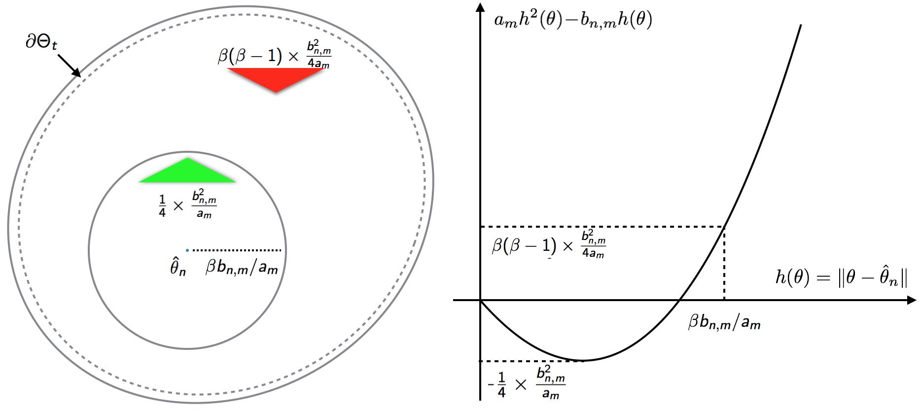
Figure 1: Intuition of Lemmas 5.1 and 5.2.

Lemma 5.2.

For any $\beta>1$, let $B=\{\theta\in\Theta:h(\theta)\leq\beta b_{n,m}/a_{m}\}$. If $a_{m}=\lambda-\sqrt{d}CL\alpha^{m}>0$ then it follows from Lemma 5.1 that both

$$\left\{\sum_{s=0}^{t-1}Y_{s+1}\mathbb{I}\left(\theta_{s}\in\partial\Theta_{s}^{c}\cap B^{c}\right)\right\}_{t\geq 0}\quad\left\{\sum_{s=0}^{t-1}Z_{s+1}\mathbb{I}\left(\theta_{s}\in\partial\Theta_{s}\cup B\right)\right\}_{t\geq 0}$$

are super-martingales (adapted to the natural filtration of $\{\theta_{t}\}_{t\geq 0}$) under $\mathbb{P}^{\mathbf{x}}$, where $Y_{t}$ and $Z_{t}$ are defined as below.

$$Y_{t+1} =h^{2}(\theta_{t+1})-h^{2}(\theta_{t})+2\eta_{t}\beta(\beta-1)b^{2}_{n,m}/a_{m}-4d\eta_{t}^{2}C^{2},$$ (16)

$$Z_{t+1} =h^{2}(\theta_{t+1})-h^{2}(\theta_{t})-\eta_{t}b^{2}_{n,m}/2a_{m}-4d\eta_{t}^{2}C^{2}.$$ (17)

6 Limiting Behaviors of $\theta_{t}$ under $\mathbb{P}^{\mathbf{x}}$

Lemma 6.1 shows that the two super-martingales constructed in Lemma 5.2 have bounded difference $\mathcal{O}(\eta_{t})$ and further by the Azuma-Hoeffding inequality [17] and Borel-Cantelli Lemma [18] that

$$\limsup_{t\to\infty}\frac{\sum_{s=0}^{t-1}Y_{s+1}\mathbb{I}\left(\theta_{s}\in\partial\Theta_{s}^{c}\cap B^{c}\right)}{\sum_{s=0}^{t-1}\eta_{s}}\leq 0,$$ (18)

$$\limsup_{t\to\infty}\frac{\sum_{s=0}^{t-1}Z_{s+1}\mathbb{I}\left(\theta_{s}\in\partial\Theta_{s}\cup B\right)}{\sum_{s=0}^{t-1}\eta_{s}}\leq 0.$$ (19)

$\mathbb{P}^{\mathbf{x}}$-almost surely. Further, (18) and (19) imply

$$\liminf_{t\to\infty}\frac{\sum_{s=0}^{t}\eta_{s}\mathbb{I}\left(\theta_{s}\in\partial\Theta_{s}\cup B\right)}{\sum_{s=0}^{t}\eta_{s}}\geq\frac{4\beta(\beta-1)}{4\beta(\beta-1)+1},$$ (20)

$\mathbb{P}^{\mathbf{x}}$-almost surely. It suggests that: if the naïve gradient descent update does not get $\theta_{t}$ stuck at the boundary of the parameter space $\Theta$, that is $\sum_{t=0}^{\infty}\mathbb{I}\left(\theta_{t}\in\partial\Theta_{t}\right)<\infty$, $\theta_{t}$ stays a large proportion of time (weighted by $\eta_{t}$) in the ball $B$.

Lemma 6.1.

Assume (A1), (A2), (A3), (A5), (A6) and that data sample $\mathbf{x}$ satisfies (12) and (13). If $\lambda-\sqrt{d}CL\alpha^{m}>0$ then (18), (19) and (20) hold $\mathbb{P}^{\mathbf{x}}$-almost surely.

Proof.

We first show the two super-martingales has bounded differences $\mathcal{O}(\eta_{t})$. Write

$$h^{2}(\theta_{t+1})-h^{2}(\theta_{t})=2\eta_{t}g_{\text{cd}}({\theta_{t}})\cdot(\theta_{t}-\hat{\theta}_{n})+\eta_{t}^{2}\|g_{\text{cd}}({\theta_{t}})\|^{2}$$

implying $|h^{2}(\theta_{t+1})-h^{2}(\theta_{t})|=\mathcal{O}(\eta_{t})$, and further $|Y_{t+1}\mathbb{I}\left(\theta_{t}\in\partial\Theta_{t}^{c}\cap B^{c}\right)|\leq H\eta_{t}$ for some constant $H>0$. Applying Azuma-Hoeffding inequality yields for any $\epsilon>0$,

$$\mathbb{P}^{\mathbf{x}}\left({\frac{\sum_{s=0}^{t-1}Y_{s+1}\mathbb{I}\left(\theta_{s}\in\partial\Theta_{s}^{c}\cap B^{c}\right)}{\sum_{s=0}^{t-1}\eta_{s}}\geq\epsilon}\right) \leq\exp{\left(-\frac{\epsilon^{2}(\sum_{s=0}^{t-1}\eta_{s})^{2}}{2H^{2}\sum_{s=0}^{t-1}\eta_{s}^{2}}\right)}$$

As assumed in (A6) $\sum_{s=0}^{\infty}\eta_{s}^{2}<\infty$, and $\sum_{s=0}^{t-1}\eta_{s}/\sqrt{\log t}\to\infty$. So the RHS $\leq\exp{(-2\log t)}=1/t^{2}$ for sufficiently large $t$ and thus is summable. Applying Borel-Cantelli Lemma yields

$$\mathbb{P}^{\mathbf{x}}\left({\frac{\sum_{s=0}^{t-1}Y_{s+1}\mathbb{I}\left(\theta_{s}\in\partial\Theta_{s}^{c}\cap B^{c}\right)}{\sum_{s=0}^{t-1}\eta_{s}}\geq\epsilon\text{ infinitely often}}\right)=0.$$

That is,

$$\limsup_{t\to\infty}\frac{\sum_{s=0}^{t-1}Y_{s+1}\mathbb{I}\left(\theta_{s}\in\partial\Theta_{s}^{c}\cap B^{c}\right)}{\sum_{s=0}^{t-1}\eta_{s}}<\epsilon$$

$\mathbb{P}^{\mathbf{x}}$-almost surely. Noting that $\epsilon$ is arbitrary, we have (18). An analogous argument obtains (19). Next, noting boundedness of $h(\theta_{t})$ and the fact that $\eta_{t}$ is not summable but square summable, we have

$$\frac{\sum_{s=0}^{t-1}Y_{s+1}}{\sum_{s=0}^{t-1}\eta_{s}}=\frac{h^{2}(\theta_{t})-h^{2}(\theta_{0})}{\sum_{s=0}^{t-1}\eta_{s}}+\frac{2\beta(\beta-1)b^{2}_{n,m}}{a_{m}}-\frac{4dC^{2}\sum_{s=0}^{t-1}\eta_{s}^{2}}{\sum_{s=0}^{t-1}\eta_{s}}\to\frac{2\beta(\beta-1)b^{2}_{n,m}}{a_{m}}$$ (21)

$\mathbb{P}^{\mathbf{x}}$-almost surely as $t\to\infty$. (18), (19), (21) and the fact that

$$(Y_{s+1}-Z_{s+1})\mathbb{I}\left(\theta_{s}\in\partial\Theta_{s}\cup B\right)=Y_{s+1}-Y_{s+1}\mathbb{I}\left(\theta_{s}\in\partial\Theta_{s}^{c}\cap B^{c}\right)-Z_{s+1}\mathbb{I}\left(\theta_{s}\in\partial\Theta_{s}\cup B\right)$$

imply

$$\liminf_{t\to\infty}\frac{\sum_{s=0}^{t-1}(Y_{s+1}-Z_{s+1})\mathbb{I}\left(\theta_{s}\in\partial\Theta_{s}\cup B\right)}{\sum_{s=0}^{t-1}\eta_{s}}\geq\frac{2\beta(\beta-1)b^{2}_{n,m}}{a_{m}}.$$

We divide both sides by $(2\beta(\beta-1)+1/2)b^{2}_{n,m}/a_{m}$ and yield (20). ∎

7 Convergence of CD to True Parameter

So far we have (20) to describe the behaviors of $\theta_{t}$ in the limit of $t\to\infty$ conditional on a particular data sample of size $n$. Lemma 7.1 follows to give an upper bound for $h(\bar{\theta}_{t})=\|\bar{\theta}_{t}-\hat{\theta}_{n}\|$ under $\mathbb{P}^{\mathbf{x}}$. Such a bound decays at a rate roughly $1/\sqrt[3]{n}$ as $n\to\infty$. The key is to let $\beta$ increase with $n$ at an appropriate rate such that the radius of $B$ vanishes as $n\to\infty$ while the proportion of time of $\theta_{t}\in B$ increases to 1. The convergence in (unconditional) probability result in Theorem 2.1 is a consequence of Lemma 7.1.

Lemma 7.1.

From Lemma 6.1, it follows that if $\lambda-\sqrt{d}CL\alpha^{m}>0$ and $\sum_{t=0}^{\infty}\mathbb{I}(\theta_{t}\in\partial\Theta_{t})<\infty$,

$$\limsup_{t\to\infty}\|\bar{\theta}_{t}-\hat{\theta}_{n}\|=\mathcal{O}(n^{-(1-2\gamma)/3})$$

$\mathbb{P}^{\mathbf{x}}$-almost surely. And the coefficient factor depends on $m$ but not data sample $\mathbf{x}$.

Proof.

Using the convexity of $h(\theta)$, (20 and the assumption $\sum_{t=0}^{\infty}\mathbb{I}(\theta_{t}\in\partial\Theta_{t})<\infty$ yields

$$\limsup_{t\to\infty}h(\bar{\theta}_{t}) \leq\limsup_{t\to\infty}\frac{\sum_{s=0}^{t}\eta_{s}h(\theta_{s})}{\sum_{s=0}^{t}\eta_{s}} h(\theta) \theta$$ [convexity of in ]

$$=\limsup_{t\to\infty}\frac{\sum_{s=0}^{t}\eta_{s}h(\theta_{s})\mathbb{I}(\theta_{s}\in B)}{\sum_{s=0}^{t}\eta_{s}}+\limsup_{t\to\infty}\frac{\sum_{s=0}^{t}\eta_{s}h(\theta_{s})\mathbb{I}(\theta_{s}\not\in B)}{\sum_{s=0}^{t}\eta_{s}}$$

$$\leq\frac{\beta b_{n,m}}{a_{m}}+\max_{\theta\in\Theta}h(\theta)\times\limsup_{t\to\infty}\frac{\sum_{s=0}^{t}\eta_{s}\mathbb{I}(\theta_{s}\not\in B)}{\sum_{s=0}^{t}\eta_{s}}$$

$$\leq\frac{\beta b_{n,m}}{a_{m}}+\max_{\theta\in\Theta}h(\theta)\times\frac{1}{4\beta(\beta-1)+1}.$$

The desired bound $\mathcal{O}(n^{-(1-2\gamma)/3})$ is obtained by letting $\beta=n^{(1-2\gamma)/6}$. If so, the radius of $B$ is $\frac{\beta b_{n,m}}{a_{m}}\asymp n^{(1-2\gamma)/6}\times n^{-1/2+\gamma}=n^{-(1-2\gamma)/3}$, and the proportion of time of $\theta_{t}\not\in B$ is at most $\frac{1}{4\beta(\beta-1)+1}\asymp n^{-(1-2\gamma)/3}$. The coefficient factor $\frac{1+\sqrt{d}CL\alpha^{m}}{\lambda-\sqrt{d}CL\alpha^{m}}+\frac{1}{4}\max_{\theta,\theta^{\prime}\in\Theta}\|\theta-\theta^{\prime}\|$ depends on $m$ but not the data sample $\mathbf{x}$. ∎

Proof of Theorem 2.1.

By Lemma 3.2,

$$\lim_{n\to\infty}\mathbb{P}\left(\left.X_{1},\dots,X_{n}\text{ satisfies (\ref{eqn: MLE}), (\ref{eqn: empirical process})}\right|\theta_{t}\in\partial\Theta_{t}\text{ finitely often}\right)=1$$

if $\mathbb{P}\left(\theta_{t}\in\partial\Theta_{t}\text{ finitely often}\right)>0$. It suffices to show that for any $\mathbf{x}$ satisfying (12) and (13)

$$\lim_{n\to\infty}\mathbb{P}^{\mathbf{x}}\left({\left.\limsup_{t\to\infty}\|\bar{\theta}_{t}-\theta^{*}\|\leq K_{m}n^{-(1-2\gamma)/3}\right|\theta_{t}\in\partial\Theta_{t}\text{ finitely often}}\right)=1$$

This is an immediate consequence of the bound $\mathcal{O}(n^{-(1-2\gamma)/3})$ given by Lemma 7.1 and the fact that

$$\|\bar{\theta}_{t}-\theta^{*}\|\leq\|\hat{\theta}_{n}-\theta^{*}\|+\|\bar{\theta}_{t}-\hat{\theta}_{n}\|\leq n^{-1/2+\gamma}+\mathcal{O}(n^{-(1-2\gamma)/3}).$$

∎

8 Example: CD for fully-visible Boltzmann Machine

An example satisfying assumptions (A1), (A2), (A3), (A4) and (A5) is Gibbs sampling with random scan for fully-visible Boltzmann Machine (details are discussed in Appendix). To demonstrate our theoretical results, we give experimental results of CD in a fully-visible $2\times 2$ Boltzmann Machine

$$p_{\theta}(x_{1},x_{2})\propto\exp{\left(\left[\begin{array}[]{c}x_{1}\\ x_{2}\end{array}\right]^{T}\left[\begin{array}[]{c c}\theta^{(1)}&\theta^{(2)}/2\\ \theta^{(2)}/2&\theta^{(3)}\end{array}\right]\left[\begin{array}[]{c}x_{1}\\ x_{2}\end{array}\right]\right)}=\exp{\left(\theta^{(1)}x_{1}^{2}+\theta^{(2)}x_{1}x_{2}+\theta^{(3)}x_{2}^{2}\right)}$$

with $x_{1},x_{2}\in\{0,1\}$. Three data sets of size $n=10^{2},10^{3},10^{4}$ are sampled with true parameter $\theta^{*}=(0.5,1.0,0.5)^{T}$. Then CD-2 and CD-4 run $t=1000$ iterations of updates with $\eta_{t}=1/t$ and generate a sequence of parameter estimates $\{\theta_{t}\}_{0\leq t\leq 1000}$. We drop the first $t_{0}=50$ estimates, and plot in Figure 2 the distance from $\bar{\theta}_{t}=\sum_{s=50}^{t}\eta_{s}\theta_{s}/\sum_{s=50}^{t}\eta_{s}$ to the true parameter $\theta^{*}$.

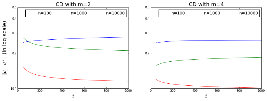
Figure 2: For each fixed $n=10^{2},10^{3},10^{4}$, $\bar{\theta}_{t}$ converges to some limit point(s) as $t\to\infty$, which is not $\theta^{*}$. But $\delta_{n}=\limsup_{t\to\infty}\|\bar{\theta}_{t}-\theta^{*}\|$ decreases as $n$ increases. The effect of $m=2$ or $4$ is not significant as it only changes the coefficient factor of the convergence rate.

9 Appendix

Proof of Lemma 3.1

Proof.

It is clearly true if $\theta_{t}\in\partial\Theta_{t}$. If $\theta_{t}\not\in\partial\Theta_{t}$, $\theta_{t+1}$ in the CD update equation (11) is function of $\theta_{t}$, $\mathbf{X}$ and a random sample $X^{(m)}_{i}$. And $X^{(m)}_{i}\sim k_{\theta_{t}}^{m}(x_{i},\cdot)$ are conditionally independent to the history of $\theta_{0},\dots,\theta_{t-1}$ given $\mathbf{X}=\mathbf{x}$ and $\theta_{t}$. For any $A\subseteq\Theta$,

$$\mathbb{P}^{\mathbf{x}}\left({\theta_{t+1}\in A|\theta_{t},\dots,\theta_{0}}\right) =\mathbb{P}\left({\theta_{t+1}\in A|\theta_{t},\dots,\theta_{0},\mathbf{X}=\mathbf{x}}\right)$$

$$=\mathbb{P}\left({\mathbf{X}^{(m)}\in g_{\text{cd}}^{-1}((A-\theta_{t})/\eta_{t})|\theta_{t},\dots,\theta_{0},\mathbf{X}=\mathbf{x}}\right)$$

$$=\mathbb{P}\left({\mathbf{X}^{(m)}\in g_{\text{cd}}^{-1}((A-\theta_{t})/\eta_{t})|\theta_{t},\mathbf{X}=\mathbf{x}}\right)$$

$$=\mathbb{P}\left({\theta_{t+1}\in A|\theta_{t},\mathbf{X}=\mathbf{x}}\right)$$

$$=\mathbb{P}^{\mathbf{x}}\left({\theta_{t+1}\in A|\theta_{t}}\right)$$

∎

Proof of Lemma 5.1

Proof.

Lemma 3.1 has shown that $\{\theta_{t}\}_{t\geq 0}$ is an inhomogeneous Markov chain. It suffices to show

$$\mathbb{E}^{\mathbf{x}}\left[{Y_{t+1}\mathbb{I}\left(\theta_{t}\in\partial\Theta_{t}^{c}\cap B^{c}\right)|\theta_{t}}\right] \geq 0,$$ (22)

$$\mathbb{E}^{\mathbf{x}}\left[{Z_{t+1}\mathbb{I}\left(\theta_{t}\in\partial\Theta_{t}\cup B\right)|\theta_{t}}\right] \geq 0.$$ (23)

Indeed, if $\theta_{t}\in\partial\Theta_{t}^{c}\cap B^{c}$ then $h(\theta_{t})\geq\beta b_{n,m}/a_{m}$ implies $a_{m}h^{2}(\theta_{t})-b_{n,m}h(\theta_{t})\geq\beta(\beta-1)b^{2}_{n,m}/a_{m}$, which together with (15) further implies

$$\mathbb{E}^{\mathbf{x}}\left[{h^{2}(\theta_{t+1})|\theta_{t}}\right]\leq h^{2}(\theta_{t})-2\beta(\beta-1)\eta_{t}b^{2}_{n,m}/a_{m}+4d\eta_{t}^{2}C^{2},$$

completing the proof of (22). Analogously, if $\theta_{t}\in B$ then $h(\theta_{t})\leq\beta b_{n,m}/a_{m}$ implies $a_{m}h^{2}(\theta_{t})-b_{n,m}h(\theta_{t})\geq-\eta_{t}b^{2}_{n,m}/4a_{m}$, which together with (15) further implies

$$\mathbb{E}^{\mathbf{x}}\left[{h^{2}(\theta_{t+1})|\theta_{t}}\right]\leq h^{2}(\theta_{t})+\eta_{t}b^{2}_{n,m}/2a_{m}+4d\eta_{t}^{2}C^{2}.$$

It with the fact that $\mathbb{E}^{\mathbf{x}}\left[{h^{2}(\theta_{t+1})|\theta_{t}}\right]=h^{2}(\theta_{t})$ if $\theta_{t}\in\partial\Theta_{t}$, completes the proof of (23). ∎

Proof of Lemma 5.2

Proof.

If $\theta_{t}\in\partial\Theta_{t}$, (15) trivially hold. If $\theta_{t}\not\in\partial\Theta_{t}$,

$$h^{2}(\theta_{t+1}) =h^{2}(\theta_{t+1}+\eta_{t}g_{\text{cd}}({\theta_{t}}))$$

$$=h^{2}(\theta_{t})+2\eta_{t}g_{\text{cd}}({\theta_{t}})\cdot(\theta_{t}-\hat{\theta}_{n})+\eta_{t}^{2}\|g_{\text{cd}}({\theta_{t}})\|^{2}$$

$$=h^{2}(\theta_{t})+2\eta_{t}g(\theta_{t})\cdot(\theta_{t}-\hat{\theta}_{n})+2\eta_{t}[g_{\text{cd}}({\theta_{t}})-g(\theta_{t})]\cdot(\theta_{t}-\hat{\theta}_{n})+\eta_{t}^{2}\|g_{\text{cd}}({\theta_{t}})\|^{2}$$

$$\leq h^{2}(\theta_{t})-2\eta_{t}\lambda h^{2}(\theta_{t})+2\eta_{t}[g_{\text{cd}}({\theta_{t}})-g(\theta_{t})]\cdot(\theta_{t}-\hat{\theta}_{n})+4d\eta_{t}^{2}C^{2}$$

where the last step follows from the facts that $g(\theta_{t})\cdot(\theta_{t}-\hat{\theta}_{n})=-(\theta_{t}-\hat{\theta}_{n})^{T}\nabla^{2}\Lambda(\theta^{\prime})(\theta_{t}-\hat{\theta}_{n})\leq-\lambda h^{2}(\theta_{t})$ with some $\theta^{\prime}$ between $\theta_{t}$ and $\hat{\theta}_{n}$ and that $\|g_{\text{cd}}({\theta})\|\leq 2\sqrt{d}C$. Taking conditional expectation $\mathbb{E}^{\mathbf{x}}\left[{\cdot|\theta_{t}}\right]$ on both sides yields

$$\mathbb{E}^{\mathbf{x}}\left[{h^{2}(\theta_{t+1})|\theta_{t}}\right] \leq h^{2}(\theta_{t})-2\eta_{t}\lambda h^{2}(\theta_{t})+2\eta_{t}\mathbb{E}^{\mathbf{x}}\left[{g_{\text{cd}}({\theta_{t}})-g(\theta_{t})|\theta_{t}}\right]\cdot(\theta_{t}-\hat{\theta}_{n})+4d\eta_{t}^{2}C^{2}$$

$$\leq h^{2}(\theta_{t})-2\eta_{t}\lambda h^{2}(\theta_{t})+2\eta_{t}\|\mathbb{E}^{\mathbf{x}}\left[{g_{\text{cd}}({\theta_{t}})-g(\theta_{t})|\theta_{t}}\right]\|\times h(\theta_{t})+4d\eta_{t}^{2}C^{2}$$

Using Lemma 4.1 and rearranging terms yields (15) as desired. ∎

Gibbs Sampling for Fully-visible Boltzmann Machine

With $x\in\{0,1\}^{p}$ and a symmetric matrix $W_{p\times p}$, fully-visible Boltzmann Machine is given by

$$p_{W}(x)\propto\exp{(x^{T}Wx)}=\exp{\left(\sum_{j=1}^{p}W_{jj}x_{j}^{2}+\sum_{1\leq j<k\leq p}2W_{jk}x_{j}x_{k}\right)}$$

which apparently belongs to an exponential family satisfying (A1) and (A3), with $d=p(p+1)/2$, $\phi(x)=(x_{j}^{2},1\leq j\leq p;x_{j}x_{k},1\leq j<k\leq p)$, $\theta=(W_{jj},1\leq j\leq p;2W_{jk},1\leq j<k\leq p)$, $C=1$. Let $\Theta$ to be the set of $\theta$ such that $W(\theta)$ has bounded Frobenius norm $\|W\|_{\text{F}}=\sqrt{\text{trace}(W^{T}W)}\leq M$, then $\Theta$ is compact as required in (A2). The probabilities $k_{\theta}(x,x^{\prime})$ of the Gibbs sampler flipping $x_{j}\to x_{j}^{\prime}$ are continuously differentiable in $\theta$ (or equivalent $W$) on compact set $\Theta$, and thus Lipchitz continuous in $\theta$. Therefore (A4) is satisfied as

$$\rho(k_{\theta},k_{\theta^{\prime}})\leq\sup_{x\in\{0,1\}^{p}}\sum_{x^{\prime}\in\{0,1\}^{p}}|k_{\theta}(x,x^{\prime})-k_{\theta^{\prime}}(x,x^{\prime})|\leq\zeta\|\theta-\theta^{\prime}\|.$$

for some $\zeta$. Moreover, a Gibbs sampler with random scan generates a uniform ergodic, reversible Markov chain which has $\mathcal{L}_{2}$-spectral gap as required in (A5).

References

- Hinton [2002] Geoffrey E Hinton. Training products of experts by minimizing contrastive divergence. Neural computation, 14(8):1771–1800, 2002.
- Hinton et al. [2006] Geoffrey E Hinton, Simon Osindero, and Yee-Whye Teh. A fast learning algorithm for deep belief nets. Neural computation, 18(7):1527–1554, 2006.
- He et al. [2004] Xuming He, Richard S Zemel, and Miguel Á Carreira-Perpiñán. Multiscale conditional random fields for image labeling. In Computer vision and pattern recognition, 2004. CVPR 2004. Proceedings of the 2004 IEEE computer society conference on, volume 2, pages II–695. IEEE, 2004.
- Roth and Black [2005] Stefan Roth and Michael J Black. Fields of experts: A framework for learning image priors. In Computer Vision and Pattern Recognition, 2005. CVPR 2005. IEEE Computer Society Conference on, volume 2, pages 860–867. IEEE, 2005.
- MacKay [2001] David MacKay. Failures of the one-step learning algorithm. In Available electronically at http://www. inference. phy. cam. ac. uk/mackay/abstracts/gbm. html. Citeseer, 2001.
- Teh et al. [2003] Yee Whye Teh, Max Welling, Simon Osindero, and Geoffrey E Hinton. Energy-based models for sparse overcomplete representations. The Journal of Machine Learning Research, 4:1235–1260, 2003.
- Williams and Agakov [2002] Christopher KI Williams and Felix V Agakov. An analysis of contrastive divergence learning in gaussian boltzmann machines. Institute for Adaptive and Neural Computation, 2002.
- Yuille [2005] Alan L Yuille. The convergence of contrastive divergences. In Advances in Neural Information Processing Systems, pages 1593–1600, 2005.
- Sutskever and Tieleman [2010] Ilya Sutskever and Tijmen Tieleman. On the convergence properties of contrastive divergence. In International Conference on Artificial Intelligence and Statistics, pages 789–795, 2010.
- Hyvärinen [2006] Aapo Hyvärinen. Consistency of pseudolikelihood estimation of fully visible boltzmann machines. Neural Computation, 18(10):2283–2292, 2006.
- Wu et al. [2016] Tung-Yu Wu, Bai Jiang, Yifan Jin, and Wing H Wong. Convergence of contrastive divergence algorithm in exponential family. arXiv preprint arXiv:1603.05729v2, 2016.
- Rudolf [2011] Daniel Rudolf. Explicit error bounds for markov chain monte carlo. arXiv preprint arXiv:1108.3201, 2011.
- Van Der Vaart and Wellner [1996] Aad W Van Der Vaart and Jon A Wellner. Weak Convergence. Springer, 1996.
- Roberts et al. [2004] Gareth O Roberts, Jeffrey S Rosenthal, et al. General state space markov chains and mcmc algorithms. Probability Surveys, 1:20–71, 2004.
- Paulin [2012] Daniel Paulin. Concentration inequalities for markov chains by marton couplings and spectral methods. arXiv preprint arXiv:1212.2015, 2012.
- Lehmann et al. [1991] Erich Leo Lehmann, George Casella, and George Casella. Theory of point estimation. Wadsworth & Brooks/Cole Advanced Books & Software, 1991.
- Azuma [1967] Kazuoki Azuma. Weighted sums of certain dependent random variables. Tohoku Mathematical Journal, Second Series, 19(3):357–367, 1967.
- Durrett [2010] Rick Durrett. Probability: theory and examples. Cambridge university press, 2010.