Light scattering from dense cold atomic media

Abstract

We theoretically study the propagation of light through a cold atomic medium, where the effects of motion, laser intensity, atomic density, and polarization can all modify the properties of the scattered light. We present two different microscopic models: the “coherent dipole model” and the “random walk model”, both suitable for modeling recent experimental work done in large atomic arrays in the low light intensity regime. We use them to compute relevant observables such as the linewidth, peak intensity and line center of the emitted light. We further develop generalized models that explicitly take into account atomic motion. Those are relevant for hotter atoms and beyond the low intensity regime. We show that atomic motion can lead to drastic dephasing and to a reduction of collective effects, together with a distortion of the lineshape. Our results are applicable to model a full gamut of quantum systems that rely on atom-light interactions including atomic clocks, quantum simulators and nanophotonic systems.

I Introduction

Light-matter interactions are fundamental for the control and manipulation of quantum systems. Thoroughly understanding them can lead to significant advancements in quantum technologies, quantum simulations, quantum information processing and precision measurements Kimble (2008); Cirac et al. (1997); De Riedmatten et al. (2008); Douglas et al. (2015); Bloch (2005); Jotzu et al. (2014); Bloch et al. (2012). Over the past decades, cold atom experiments have provided a clean and tunable platform for studying light-matter interactions in microscopic systems where rich quantum effects emerge, such as superradiance and subradiance, electromagnetically induced transparency, and non-classical states of light Bohnet et al. (2012); Guerin et al. (2016); Safavi-Naeini et al. (2011); Ourjoumtsev et al. (2011); Brooks et al. (2012). However, in spite of intensive theoretical and experimental efforts over the years, long-standing open questions still remain regarding the propagation of light through a coherent medium, especially when it consists of large and dense ensembles of scatterers James (1993); Lehmberg (1970); Ruostekoski and Javanainen (1997); Javanainen et al. (1999); Scully et al. (2006); Svidzinsky et al. (2010); Bienaimé et al. (2012); Sokolov et al. (2013); Javanainen et al. (2014); Sokolov (2015); Olave et al. (2015); Jennewein et al. (2015a); Javanainen and Ruostekoski (2016); Jenkins et al. (2016); Araújo et al. (2016). In fact, by studying small systems where analytical solutions are obtainable, it has been realized that atom-atom interactions can significantly modify the spectral characteristics of the emitted light. These effects yet need to be understood in large systems Olmos et al. (2013); Maier et al. (2014); Yu (2015); Zhu et al. (2015); Bettles et al. (2015) where finite size effects and boundary conditions become irrelevant. The situation is even more complicated when the coupling with atomic motion is non-negligible Berman (1997); Li et al. (2013). It is timely to develop theories capable of addressing these questions, given the rapid developments on cold atom experiments and nanophotonic systems. The experiments are entering strongly coupled regimes, where atom-atom and atom-photon interactions need to be treated simultaneously and sometimes fully microscopically Olmos et al. (2013); Jennewein et al. (2015b); Goldschmidt et al. (2015).

A widely adopted approach to describe light scattering consists of integrating out the atomic degrees of freedom and treating the atoms just as random scatterers with prescribed polarizability de Vries et al. (1998); van Rossum and Nieuwenhuizen (1999); Labeyrie et al. (2003); Brown and Mortensen (2000). While this approach can successfully capture some classical properties of the scattered light, it does not fully treat the roles of atom-atom interactions and atomic motion Labeyrie et al. (1999); Labeyrie et al. (2004a); Sigwarth et al. (2004); Labeyrie et al. (2006). An alternative route consists of tracing over the photonic degrees of freedom. In this case the virtual exchange of photons induces dispersive and dissipative dipole-dipole interactions between atoms, which can be accounted for by a master equation formulation James (1993); Lehmberg (1970). This approach has been used to study systems of tightly localized atoms where the dynamics only takes place in the atomic internal degrees of freedom. It has been shown to successfully capture quantum effects in light scattering Svidzinsky et al. (2010); Chomaz et al. (2012); Yu (2014); Bienaimé et al. (2012, 2014); Sutherland and Robicheaux (2016). However, due to the computational complexity, it has been often restricted to weak excitation and small samples Miroshnychenko et al. (2013); Meir et al. (2014); Yu (2015); Zhu et al. (2015), and a direct comparison with experiments containing a large number of atoms has been accomplished only recently Bromley et al. (2016); Roof et al. (2016). In general, most theories have not properly accounted for atomic motional effects and atomic interactions on the same footing and many open questions in light scattering processes remain.

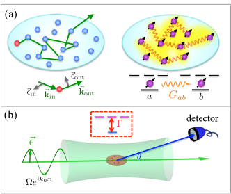
Figure 1: (Color online) Scheme. (a) Microscopic models: random walk model (left) and coherent dipole (right). In the random walk model, a photon is randomly scattered by the atoms. Scattering events are characterized by the incident and outgoing wavevector of the photons and their corresponding polarization. In the coherent dipole model, atoms are coupled by dipole-dipole interactions ($G_{ab}$) and all atoms contribute to the fluorescence. (b) Experimental setup for measuring the fluorescence from a cloud of atoms. An incident laser drives an atomic transition with a spontaneous emission rate $\Gamma$. Atoms absorb and emit light. The detectors collect scattered photons at an angle $\theta$ measured from the incident beam direction.

Here, we present a unifying theoretical framework based on a coherent dipole (CD) model (see Fig. 1(a)) to study the light scattering from cold atoms with possible residual motion. In the low intensity and slow motion regime, we use the CD to investigate the collective effects in the light scattered by a large cloud and show the interplay of optical depth and density. These results are compared with the random walk (RW) model (see Fig. 1(a)) that only accounts for incoherent scattering and thus ignores coherent dipolar interaction effects. To address the role of atomic motion, we perform different levels of generalization of the CD model. With these modified models, we show that atomic motion not only reduces phase coherence and collective effects, but also impacts the lineshape and linecenter of the spectral emission lines via photon recoils. Motivated by a recent experiment at JILA (see Fig. 1(b)) Bromley et al. (2016), we focus our discussions on a $J=0\rightarrow J=1$ transition, but the methods presented here can be extended to more complicated level structures without much difficulty.

This paper is organized as follows. In Sec. II, we provide the mathematical description of the CD model, which treats atoms as coupled, spatially fixed dipoles sharing a single excitation. Its predictions on the collective properties of the emitted light such as the light polarization and density dependence of the lineshape and peak intensity are discussed. In Sec. III, we introduce the RW model and compare its predictions on the linewidth and peak intensity of the scattered light to the ones obtained from the CD model. Those comparisons allow us to explore the role of phase coherence in the atom-light interaction. In Sec. IV, we present extended models to study motional effects on atomic emission. We first include motion in the CD model by assuming that its leading contributions comes from Doppler shifts. Those are accounted for in the frozen model approximation when we introduce local random detunings for atoms sampled from a Maxwell-Boltzmann distribution. Then we go beyond the frozen model approximation and explicitly include atomic motion by means of a semi-classical approach. This treatment also allow us to go beyond the low excitation regime. We finish in Sec. V with conclusions and and outlook.

II Coherent dipole model

II.1 Equations of motion for coherent dipoles

For an ensemble of $N$ atoms with internal dipole transition $J=0\rightarrow J^{\prime}=1$, the Hamiltonian of the system that includes the interaction between atoms and the radiation field is Gross and Haroche (1982)

$$H = \hbar\sum_{{\bf k},\bm{\epsilon}}\omega_{k}\hat{a}^{\dagger}_{{\bf k}\bm{\epsilon}}\hat{a}_{{\bf k}\bm{\epsilon}}+\hbar\sum_{i,\alpha}\omega_{\alpha}\hat{b}_{i}^{\alpha\dagger}\hat{b}_{i}^{\alpha}+\sum_{i}\hat{\bf D}_{i}\cdot\hat{\bf E}({\bf r}),$$

$$\hat{D}_{i}^{\alpha} = d(\hat{b}_{i}^{\alpha\dagger}+\hat{b}_{i}^{\alpha}),$$ (2)

$$\hat{\bf E}({\bf r}) = \sum_{{\bf k}{\bm{\epsilon}}}g_{k}\bm{\epsilon}_{\bf k}(e^{i{\bf k}\cdot{\bf r}}\hat{a}_{{\bf k}\bm{\epsilon}}+\mathrm{H.c.}),$$ (3)

where we have used the notation $\ket{\alpha}$ to denote the excited levels, and $\ket{0}$ for the lower state. For convenience, we choose the Cartesian basis, $\ket{\alpha}=\ket{x},\ket{y}$ or $\ket{z}$. $\hat{b}_{i}^{\alpha\dagger}=\ket{\alpha_{i}}\bra{0_{i}}$ is the raising operator for transition to state $\ket{\alpha}$ of the $i^{\mathrm{th}}$ atom, and $d$ is the atomic dipole moment. The field coupling strength is denoted by $g_{k}=\sqrt{\frac{\hbar\omega_{k}}{2\varepsilon_{0}V}}$, ${\bf k}~{}(\bm{\epsilon})$ is the wavevector (polarization) of the photons, $\omega_{k}$ is the frequency of the photons, $\varepsilon_{0}$ is the vacuum permitivity, and $V$ is the photon quantization volume. Under the Born-Markov approximation, the photon degrees of freedom, $\hat{a}_{\bf k\epsilon}$, can be adiabatically eliminated, leading to a master equation for the reduced density matrix ($\hat{\rho}$) of the atoms Gross and Haroche (1982); James (1993); Olmos et al. (2013) where the effective role of the scattered photons is to mediate dipole-dipole interactions between atoms. The master equation for $\hat{\rho}$ is

$$i\frac{d\hat{\rho}}{dt} = -\sum_{i,\alpha}\Delta^{\alpha}\ket{\alpha_{i}}\bra{\alpha_{i}}+\sum_{i,\alpha}\Omega^{\alpha}(e^{i{\bf k}_{0}\cdot{\bf r}_{i}}\hat{b}_{i}^{\alpha\dagger}+\mathrm{H.c.})$$

$$+\sum_{i\neq j,\alpha,\alpha^{\prime}}g_{i,j}^{\alpha\alpha^{\prime}}[\hat{b}_{i}^{\alpha\dagger}\hat{b}_{j}^{\alpha^{\prime}},\hat{\rho}]+\sum_{i,j,\alpha,\alpha^{\prime}}f_{i,j}^{\alpha\alpha^{\prime}}[[\hat{b}_{i}^{\alpha\dagger},\hat{\rho}],\hat{b}_{j}^{\alpha^{\prime}}],$$

where we have added the term describing the effect of an external driving laser with polarization $\alpha$, wavevector ${\bf k}_{0}$, and Rabi frequency $\Omega^{\alpha}$. The Hamiltonian is written in the rotating frame of the laser, with $\Delta^{\alpha}$ denoting the detuning between the laser and the transition $\ket{0}\rightarrow\ket{\alpha}$. The dipole-dipole interactions are given by James (1993); Olmos et al. (2013)

$$G_{ij}^{\alpha\alpha^{\prime}} = \frac{3\Gamma}{4}[\delta_{\alpha,\alpha^{\prime}}A(r_{ij})+\hat{\bf r}_{ij}^{\alpha}\hat{\bf r}_{ij}^{\alpha^{\prime}}B(r_{ij})],$$ (5)

$$A(r) = -\frac{e^{ik_{0}r}}{k_{0}r}-i\frac{e^{ik_{0}r}}{k_{0}^{2}r^{2}}+\frac{e^{ik_{0}r}}{k_{0}^{3}r^{3}},$$ (6)

$$B(r) = \frac{e^{ik_{0}r}}{k_{0}r}+3i\frac{e^{ik_{0}r}}{k_{0}^{2}r^{2}}-3\frac{e^{ik_{0}r}}{k_{0}^{3}r^{3}},$$ (7)

$$g_{ij}^{\alpha\alpha^{\prime}} = \Re[G_{ij}^{\alpha\alpha^{\prime}}],$$ (8)

$$f_{ij}^{\alpha\alpha^{\prime}} = \Im[G_{ij}^{\alpha\alpha^{\prime}}],$$ (9)

where $\delta_{\alpha,\alpha^{\prime}}$ is the Kronecker delta symbol, ${\bf r}_{ij}$ is the relative seperation between the atoms $i$ and $j$, and $\hat{\bf r}^{\alpha}={\bf r}^{\alpha}/r$ denotes the component of the unit vector ${\bf r}/r$ along the direction $\alpha=x,y$ or $z$. The real and imaginary parts describe the dispersive and dissipative interactions, respectively. The spontaneous emission rate is $\Gamma=\frac{k_{0}^{3}d^{2}}{3\pi\hbar\varepsilon_{0}}$, and $k_{0}=2\pi/\lambda$ is the wavevector of the dipole transition. The dipole-dipole interactions include both the far-field ($1/r$) and near-field ($1/r^{2},1/r^{3}$) contributions. The imaginary part encapsulates collective dissipative process responsible for the superradiant emission in a dense sample. The real part accounts for elastic interactions between atoms which can give rise to coherent dynamical evolution. These elastic interactions compete with and can even destroy the superradiant emission Friedberg et al. (1972); Zhu et al. (2015).

When the atoms’ thermal velocity $v$ satisfies $k_{0}v\ll\Gamma$, atoms can be assumed to be frozen during the radiation process. Moreover, in the weak driving regime, $\Omega\ll\Gamma$, to an excellent approximation, the master equation dynamics can be captured by the $3N$ linear equations describing the atomic coherences $b_{j}^{\alpha}=\langle\hat{b}_{j}^{\alpha}\rangle$ of an excitation propagating through the ground state atomic medium. The corresponding steady state solution can be found from:

$$b_{j}^{\alpha} = \frac{\Omega^{\alpha}\delta_{\alpha,\gamma}e^{i{\bf k}_{0}\cdot{\bf r}_{j}}/2}{\Delta^{\alpha}+i\Gamma/2}+\sum_{n\neq j,\alpha^{\prime}}\frac{G_{jn}^{\alpha\alpha^{\prime}}}{\Delta^{\alpha}+i\Gamma/2}b_{n}^{\alpha^{\prime}},$$ (10)

where we have specified the polarization of the driving laser to be along $\gamma$. The fluorescence intensity measured at the position ${\bf r}_{s}$ in the far-field can be obtained by the summation James (1993)

$$I({\bf r}_{s})\propto\sum_{jn}e^{-i{\bf k}_{s}\cdot{\bf r}_{jn}}\sum_{\alpha,\alpha^{\prime}}(\delta_{\alpha,\alpha^{\prime}}-\hat{\bf r}_{s}^{\alpha}\hat{\bf r}_{s}^{\alpha^{\prime}})b_{j}^{\alpha^{\prime}}b_{n}^{\alpha*},$$ (11)

where $b_{n}^{\alpha*}$ is the complex conjugate of $b_{n}^{\alpha}$, and ${\bf r}_{jn}={\bf r}_{j}-{\bf r}_{n}$.

II.2 Collective effects in fluorescence

For dilute samples the dipolar interactions are weak, $\mathcal{G}\equiv\sum_{i\neq j,\alpha,\alpha^{\prime}}|G^{\alpha\alpha^{\prime}}_{ij}|/(N\Gamma)\ll 1$, and Eq. (10) can be solved perturbatively using $\mathcal{G}$ as an the expansion parameter, $b_{j}^{\alpha}=b_{j}^{\alpha,0}+b_{j}^{\alpha,1}+b_{j}^{\alpha,2}+...$, ($b_{j}^{\alpha,n}\propto\mathcal{G}^{n}$) which results in

$$b_{j}^{\alpha,n} = \sum_{\mathclap{\begin{subarray}{c}l_{1}\neq j\\ l_{2}\neq l_{1}\\ ...l_{n}\neq l_{n-1}\\ \alpha_{1},\alpha_{2}...\alpha_{n}\end{subarray}}}\frac{G_{jl_{1}}^{\alpha\alpha_{1}}G_{l_{1}l_{2}}^{\alpha_{1}\alpha_{2}}...G_{l_{n-1}l_{n}}^{\alpha_{n-1}\alpha_{n}}\Omega^{\gamma}\delta_{\alpha_{n},\gamma}e^{i{\bf k}_{0}\cdot{\bf r}_{l_{n}}}}{i^{n}(\Delta^{\alpha}+i\frac{\Gamma}{2})(\Delta^{\alpha_{1}}+i\frac{\Gamma}{2})...(\Delta^{\alpha_{n}}+i\frac{\Gamma}{2})}.$$ (12)

In the expansion, terms of order $n$ account for $n^{\rm th}$ order scattering events. For simplicity, in the following we assume the atomic sample has a spherical shape, with density distribution $n(r)=n_{0}e^{-r^{2}/2R^{2}}$, unless otherwise specified. However, the conclusions can be generalized to other geometries. Here, $n_{0}=\frac{N}{2\pi\sqrt{2\pi}R^{3}}$ is the peak density.

To the zeroth order, the atomic response is driven by the external field only and is not modified by the scattered light:

$$b_{j}^{\alpha,0}=\frac{\Omega^{\alpha}\delta_{\alpha,\gamma}e^{i{\bf k}_{0}\cdot{\bf r}_{j}}}{\Delta^{\alpha}+i\Gamma/2}.$$ (13)

Substituting it into Eq. (11), the intensity of scattered light is

$$I\propto N+N^{2}e^{-|{\bf k}_{s}-{\bf k}_{0}|^{2}R^{2}}.$$ (14)

There are two contributions to the intensity, the first term $\propto N$ represents the incoherent contribution, and the second term $\propto N^{2}$ is the collective emission resulting from coherent scattering processesScully et al. (2006); Bromley et al. (2016). The phase coherence is restricted to a narrow angular region around the incident laser direction, with $\delta\theta\sim 1/k_{0}R$. The enhanced emission arises from the constructive interference of the radiation from $N$ dipoles Bienaimé et al. (2014). Along other directions, the random distribution of atom positions randomizes the phases of the emitted light, smearing out the phase coherence after averaging over the whole sample Bromley et al. (2016).

Including first order corrections, the intensity of the scattered light is given by

$$I(r_{s}) \propto \frac{N\Omega^{2}}{(\Delta-\Gamma\Re[\overline{G}])^{2}+(\Gamma+2\Gamma\Im[\overline{G}])^{2}/4},$$ (15)

for transverse directions, where we have denoted $\Omega=\Omega^{\gamma}$ and $\Delta=\Delta^{\gamma}$, and $\overline{G}=\sum_{i\neq j}G_{ij}^{\gamma\gamma}e^{-i{\bf k}_{0}\cdot{{\bf r}_{ij}}}/(N\Gamma)$. For the forward direction, the intensity has the same form, except that the factor $N$ is replaced by $N^{2}$, due to the phase coherence. Therefore, the lineshape of the scattered light is Lorentzian, with its line center frequency shifted by the elastic interactions, and the linewidth broadened by the radiative interactions. If we temporarily neglect the effect of polarization, when the atom-atom separation is large, the dipole-dipole interaction is dominated by far-field terms, i. e., $G_{ij}^{\gamma\gamma}\sim-\frac{3\Gamma}{4}(1-\hat{\bf r}_{ij}^{\gamma}\hat{\bf r}_{ij}^{\gamma})\frac{e^{ik_{0}r_{ij}}}{k_{0}r_{ij}}$. In this limit analytical expressions for the linewidth broadening $\overline{\Gamma}$, and density shift, $\overline{\Delta}$, can be obtained: $\overline{\Gamma}=2\Gamma\Im[\overline{G}]=3N\Gamma/(8k_{0}^{2}R^{2})=\frac{\rm OD}{4}\Gamma$, with ${\rm OD}=\frac{3N}{2k_{0}^{2}R^{2}}$ the optical depth of the sample (see Appendix A), and $\overline{\Delta}=\Gamma\Re[\overline{G}]=-\Gamma n_{0}k_{0}^{-3}/4\sqrt{2\pi}$. Therefore, while the collectively broadened linewidth depends on the OD of the atomic cloud, the frequency shift depends on the density.

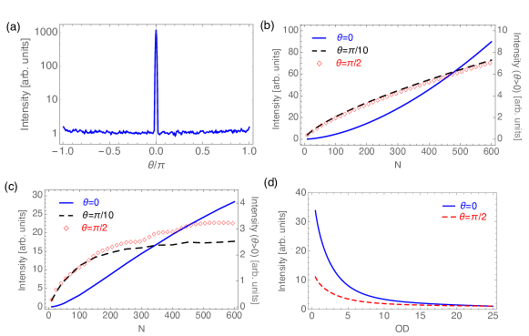
Figure 2: (Color online) CD Model: on-resonance intensity. (a) Angular distribution: due to the constructive interference along the forward direction ($\theta=0$), the intensity is drastically enhanced within a small angular region. (b)-(c) The intensities for three different directions ($\theta=0,\pi/10,\pi/2$) are shown as a function of atom number, each normalized to the value at $N=50$. All are calculated for a spherical cloud of fixed size. The right vertical axes label the intensity for $\theta=\pi/2,\pi/10$. In (b) the OD and the density are relatively low (when $N=500$, OD=2,$n_{0}k_{0}^{-3}$=0.0015). The transverse intensity increases $\sim N$, while the forward intensity increases $\sim N^{2}$, showing a collective enhancement for small window of $\theta$ around zero. Outside this narrow angular window the enhancement disappears and the intensity becomes almost $\theta$ independent as indicated by the identical behavior observed for two different angles, $\theta=\pi/10$ and $\pi/2$. In (c) the OD and density are relatively large (when $N=500$, OD=10, $n_{0}k_{0}^{-3}$=0.017). The rate at which the intensity increases with $N$ slows down in both the forward and transverse direction: with $I\sim N^{1}$ for $\theta=0$ and $I\sim N^{0.5}$ for $\theta=\pi/2$, respectively. (d) On-resonance intensity as a function of OD: it is highly suppresed at large OD. Here, the intensity is normalized to the corresponding value at ${\rm OD}=25$ for each direction.

In a dense medium dipolar interactions are strong, $\mathcal{G}\gtrsim 1$, higher order scattering events become important, and the interplay between the radiative interactions and elastic interactions becomes non-negligible. As a consequence the above perturbative analysis is no longer applicable. In Fig. 2 and Fig. 3, we show the numerical solution of Eq. (10), which takes into account all the scattering orders. As shown in Fig. 2(a), most of the scattered light is distributed within a narrow peak around the forward direction (laser direction). Outside this narrow region fluorescence is almost uniformly distributed among other directions fno (a). The forward emission is collectively enhanced. For low OD it increases as $\sim N^{2}$ (Fig. 2 (b)) while the transverse intensity increases as $\sim N$.

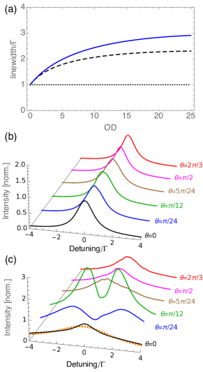
Figure 3: (Color online) CD Model: collective broadening. (a) FWHM linewidth as a function of OD. At small OD, the FWHM increases linearly with OD, but as OD increases density effects set in, multiple scattering events become relevant and the linewidth dependence on OD is no longer linear. Two different atom numbers are used for the blue (N=1000) and black lines (N=200), and the OD is varied by changing the cloud size. For the blue line, $n_{0}k_{0}^{-3}=0.14$ at OD=25, $0.003$ at OD=2. For the black line, the density at the same OD is doubled. With smaller density, the linewidth increases to a larger value in the large OD regime. (b) The lineshape at small OD values (OD=2, $n_{0}k_{0}^{-3}=0.002$) for different angles $\theta$ ($\theta$ is defined in Fig. 1(a)) is mainly Lorentzian. Here the intensity is normalized to the on-resonance intensity for each $\theta$. (c) At large OD (OD=20, $n_{0}k_{0}^{-3}=0.06$), the fluorescence lineshape significantly broadens and stops being Lorentzian. The brown dots for $\theta=0$ show the Lorentzian fit, which fails to describe the lineshape. At intermediate $\theta$, a double-peak structure shows up. For all panels, the cloud shape is spherical.

Dipolar interactions tend to suppress the rate at which the intensity grows with $N$ (Fig. 2(c)). This can be qualitatively understood from Eq. (15), which predicts that the intensity is reduced as OD increases. Despite the fact that the perturbative analysis is only valid in the weak interaction limit, this tendency remains and becomes more pronounced in the large OD regime as shown by the numerical solution presented in Fig. 2(d). Broadly speaking, multiple scattering events tend to suppress collective behavior Javanainen et al. (2014); Lagendijk and Van Tiggelen (1996). Similar physics is also observed in the behavior of the linewidth. At small OD, the FWHM linewidth increases linearly with OD (Fig. 3(a)) and the lineshape is well described by a Lorentzian (Fig. 3(b)), as expected from Eq. (15). However, when OD is large and the density is high, in addition to a significant broadening, the lineshape becomes non-Lorentzian (Fig. 3(c)) and the FWHM increases slowly with OD (Fig. 3(a)). To further illustrate this, in Fig. 3(a) we plot the FWHM for the same OD but with smaller density (by using a larger atom number). The figure shows that the linewidth indeed keeps increasing until saturation at a larger value of OD. Another interesting feature is the double-peak structure for intermediate angles $\theta$, arising due to the competition between interference and multiple scattering events (Fig. 3(c)).

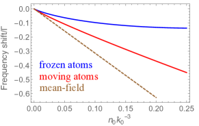
Figure 4: Color online) CD Model: frequency shift. For small density, the shift calculated from the coherent dipole model (blue line) increases linearly with density as predicted by the mean-field theory. However, when density is large, there is a significant deviation from the mean-field result. When motional effects are taken into account (red line, Doppler width $=5\Gamma$, see Sec. IV.1), the non linear suppression of the frequency shift with density is less severe.

The drastic modifications of the perturbative expectations from multiple scattering are also present in the frequency shift of the scattered light. From a mean-field point of view, the linecenter of scattered light is shifted according to the Lorentz-Lorenz shift $\pi n_{0}k_{0}^{-3}\Gamma$ Friedberg et al. (1973). As shown by the numerical calculation in Fig. 4 (blue line), at small density, the frequency shift is indeed linear with $n_{0}k_{0}^{-3}$, but as density increases, the shift is quickly suppressed Javanainen et al. (2014). For atom density $\sim 5\times 10^{13}$cm^-3 (reached for example in cold ⁸⁷Rb atom experiments Balik et al. (2013)), the calculated density shift is approximately a factor of two lower than the mean-field prediction.

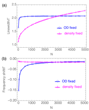
Figure 5: (Color online) CD Model: finite size scaling. (a) The linewidth is calculated for different number of atoms at the same OD (OD=4 for $N$=3000) by varying the density (blue line with circles). From $N=1000\sim 5000$ the linewidth is not obviously changed. In contrast, by keeping the same density ($n_{0}k_{0}^{-3}=0.0037$ for $N$=3000) while varying the OD (magenta line with triangles), the linewidth keeps changing. (b) The frequency shift is calculated for different number of atoms. By keeping constant density (magenta line with triangles), the frequency shift remains almost constant, while for constant OD (blue line with circles), there is a significant variation of the frequency shift with $N$. Here the cloud aspect ratio is $R_{x}:R_{y}:R_{z}=2:2:1$ Bromley et al. (2016).

The interplay between the imaginary and real part of the dipole-dipole interaction has to be carefully accounted for to compare numerical simulations with experimental measurements by doing finite size scaling. For typical computation resources the numerical solution of Eq. (10) is limited to $\sim 10^{4}$ atoms. On the other hand experiments usually operate with ensembles of tens of millions of atoms. To theoretically model these large systems a proper rescaling in the cloud size is necessary. Equation (15) implies that in order to characterize the effect of radiative interactions one should aim to match the experimental OD, which scales as $\sim N^{1/2}$. On the other hand, to properly reproduce the effect of elastic interactions it is better to match the dimensionless number $n_{0}k_{0}^{-3}$, which scales as $N^{1/3}$. Therefore, there exist two different ways of rescaling the cloud size, either by keeping the same OD or the same density. In Fig. 5 we show the effect of finite $N$ for a moderate range of atom numbers. Indeed, except from small deviations seen at very low atom number ($<1000$), the linewidth broadening can be well captured by keeping the OD constant, while the frequency shift is well described by using a constant density. In contrast, if a constant OD is used to compute the frequency shift, the result would considerablly overestimate the shift, e.g., by a factor of 10 when the $N$ in numerical simulation is 1/100 the atom number in experiment. The interplay of multiple scattering and density effects is more prominent for larger $N$ values. To deal with the OD vs density scaling issues in comparing with experiments the most appropriate rescaling procedure that we found is the following: when computing the linewidth or peak intensity, the theory is rescaled accordingly with the experimental OD. However, the actual OD value is not exactly matched to the experimental one but to a slightly modified value, $\widetilde{\rm OD}=\eta{\rm OD}$ to account for density effects Bromley et al. (2016). For a moderate window of ${\rm OD}$ values, for example achieved experimentally by letting the cloud expand for different times, $\eta$ should be kept fixed. For the frequency shift the theory should be rescaled according to density.

II.3 Anisotropic features of scattered light

For independent atoms radiation along the polarization of the driving laser is forbidden. However, dipole-dipole interactions can generate polarization components different to the driven ones if the atoms exhibit internal level structure, e.g., degenerate Zeeman levels in the excited state. This is the case of a $J=0\rightarrow J^{\prime}=1$ transition, where, as shown in Fig. 6, the fluorescence emitted along the laser polarization direction (z-direction, $\theta=\pi/2$ ) is nonzero. It is, however, much weaker than the intensity emitted along other directions. On the contrary, for two-level transitions the polarization of the scattered light is conserved and thus the emission parallel to the laser polarization is completely suppressed. The strong dependence of the scattered light on polarization and atomic internal structure is most relevant along the transverse direction. Along the forward direction those effects are irrelevant, as verified by our numerical simulations. From Eq. (12), the lowest order contribution to the intensity detected along the laser polarization direction comes from the first order scattering processes, thus $I\propto\frac{1}{(\Delta^{2}+\Gamma^{2}/4)^{2}}$, which lead to a “subradiant” lineshape (i. e. the full width at half maximum (FWHM), $\overline{\Gamma}_{\rm FWHM}=\sqrt{\sqrt{2}-1}\Gamma<\Gamma,$ is smaller than the one for independent particles). The analytic result agrees perfectly with the numerical simulation at low OD (Fig. 6(b)). As the OD increases and interactions become stronger, higher order scattering contributions lead to a collective broadening (linewidth larger than $\Gamma$) even along this “single dipole forbidden” direction, as shown in Fig. (6 (c)).

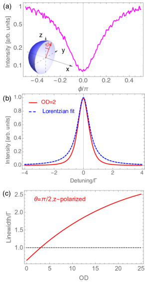
Figure 6: (Color online) CD Model: effect of laser polarization. (a) Intensity distribution in the plane perpendicular to the laser propagation direction, i. e., $\theta=\pi/2$ for all $\phi$’s (inset shows the geometry). $\phi=0$ is the z-direction. Here, the incident laser is polarized along z. The intensity detected along the laser polarization is suppressed compared to other directions. Panels (b)(c) show the lineshape and linewidth of light detected at $\theta=\pi/2,\phi=0$. (b) At small OD, the FWHM linewidth is below the natural linewidth. (c) As OD increases, the linewidth is collectively broadened due to multiple scattering processes (Fig. 3(a)). For all panels, degeneracy in excited levels has been assumed.

III Random walk model

In this section we use the random walk model to investigate the role of incoherent scattering processes in collective emission. We focus on the low-intensity regime. Classically, light transport in a disordered medium can be described by a sequence of random scattering events experienced by a photon (see Fig. 1(a)) Labeyrie et al. (2003); Labeyrie et al. (2004b); Lagendijk and Van Tiggelen (1996). The expected number of scattering events is roughly given by $({\rm OD}_{p})^{2}$, where ${\rm OD}_{p}$ is the peak optical depth, which depends on detuning $\Delta$ as $3N/[k_{0}^{2}R^{2}(1+4\Delta^{2}/\Gamma^{2})]$ . For simplicity here we also assume a spherical cloud. The transmission of light is given by $e^{-{\rm OD}_{p}}$ fno (b); Chabé et al. (2014). For the $J=0\rightarrow J^{\prime}=1$ transition (degenerated $J^{\prime}=1$ states), the differential scattering cross section that defines a scattering event is given by Labeyrie et al. (2003); Lagendijk and Van Tiggelen (1996)

$$\frac{d\sigma}{d\Omega}({\bf k}_{\rm in},\bm{\epsilon}_{\rm in}\rightarrow{\bf k}_{\rm out},\bm{\epsilon}_{\rm out}) = \frac{3\sigma_{0}}{8\pi}|\bm{\epsilon}_{\rm in}^{*}\cdot\bm{\epsilon}_{\rm out}|^{2},$$ (16)

where ${\bf k}_{\rm in,out}$ is the incident/scattered wavevector, $\bm{\epsilon}_{\rm in,out}$ is the polarization of the incident/scattered photon Labeyrie et al. (2003); Lagendijk and Van Tiggelen (1996); Raković et al. (1999) and $\sigma_{0}=3\lambda^{2}/[2\pi(1+4\Delta^{2}/\Gamma^{2})]$, with $\lambda$ the wavelength of the driving laser.

To simulate the polarization dependent scattering events as dictated by Eq. (16), it is convenient to use the Stokes-Mueller formalism Hovenier et al. (2004). A photon in a given state of polarization can be described by a Stokes vector Brosseau (1998)

$${\bf S} = \left(\begin{array}[]{lcr}S_{0}\\ S_{1}\\ S_{2}\\ S_{3}\end{array}\right)=\left({\begin{array}[]{c}\overline{|E_{l}|^{2}}+\overline{|E_{r}|^{2}}\\ \overline{|E_{l}|^{2}}-\overline{|E_{r}|^{2}}\\ \overline{E_{l}^{*}E_{r}}+\overline{E_{l}E_{r}^{*}}\\ i(\overline{E_{l}^{*}E_{r}}-\overline{E_{l}E_{r}^{*}})\end{array}}\right),$$ (25)

where $E_{l}$, $E_{r}$ are the electric field components projected onto the two orthorgonal axis $\hat{e}_{l}$ and $\hat{e}_{r}$ in the plane perpendicular to the wavevector ${\bf k}$. For example, ${\bf S}=(1,1,0,0)$ represents a photon linearly polarized along the reference axis $\hat{e}_{l}$. A scattering event ${\bf k}_{\rm in},\bm{\epsilon}_{\rm in}\rightarrow{\bf k}_{\rm out},\bm{\epsilon}_{\rm out}$ can be determined by two angles: $\theta$ and $\phi$ [see Fig. 7]. The change of polarization can be obtained from the transformation ${\bf S}^{\prime\prime}=M(\theta)\mathcal{R}(\phi){\bf S}^{\rm in}$, where ${\bf S}^{\rm in}$ is the incident Stokes vector, ${\bf S}^{\prime\prime}$ is defined with respect to the axis $\hat{e}_{l}^{\prime\prime}$, $\hat{e}_{r}^{\prime\prime}$ and $\hat{e}_{3}^{\prime\prime}$, and then ${\bf S}^{\rm out}=\mathcal{R}(\psi){\bf S}^{\prime\prime}$ transforming back to the original frame $\hat{e}_{l}$, $\hat{e}_{r}$ and $\hat{e}_{3}$ Bartel and Hielscher (2000), with ${\bf S}^{\rm out}$ the scattered Stokes vectors. The scattering matrix that we use, $M$, is the scattering matrix that describes Rayleigh scattering Hovenier et al. (2004); Lagendijk and Van Tiggelen (1996). It is given by

$${M(\theta)} = \frac{3}{4}\begin{pmatrix}{\rm cos}^{2}\theta+1&{\rm cos}^{2}\theta-1&0&0\\ {\rm cos}^{2}\theta-1&{\rm cos}^{2}\theta+1&0&0\\ 0&0&2{\rm cos}\theta&0\\ 0&0&0&2{\rm cos}\theta\end{pmatrix}.$$ (26)

The matrix, $\mathcal{R}(\phi)$, is the rotation matrix that rotates the incident axis $\hat{e}_{r}$ to $\hat{e}_{r}^{\prime}$ (perpendicular to the scattering plane),

$${\mathcal{R}(\phi)} = \begin{pmatrix}1&0&0&0\\ 0&{\rm cos}(2\phi)&{\rm sin}(2\phi)&0\\ 0&-{\rm sin}(2\phi)&{\rm cos}(2\phi)&0\\ 0&0&0&1\end{pmatrix}$$ (27)

and $\mathcal{R}(\psi)$ is the rotation matrix that transforms the coordinate system $\hat{e}_{l}^{\prime\prime}$, $\hat{e}_{r}^{\prime\prime}$ and $\hat{e}_{3}^{\prime\prime}$ back to the original coordinate system $\hat{e}_{l}$,$\hat{e}_{r}$ and $\hat{e}_{3}$, and can be found from $\theta$ and $\phi$. The polarization of the photons is encoded in the Stokes vector. The probability of a scattering event can be directly calculated from $S^{\prime\prime}_{0}/S^{\rm in}_{0}$. Complete trajectories of the photons can be found from Monte Carlo sampling of scattering events. As the phase information of photon is not kept in this approach, it is more suitable for describing classical media or hot atoms where phase coherence is not important.

The polarization of the incident photon is randomized after multiple scattering events. Since the intensity detected along the polarization direction of the incident photon requires at least two scattering events, it is suppressed compared to other directions but nonzero (Fig. 8(a)) and the linewidth at small ${\rm OD}_{p}$ also drops below the natural linewidth (Fig. 8(c)) along this direction. For the other directions, the intensity distribution is roughly homogeneous and does not exhibit the collective enhancement along the forward direction observed in the coherent dipole model. The FWHM linewidth for different directions increases linearly with OD up to a moderate value of OD (see Fig. 8(b)), and displays a polarization dependence similar to the prediction of CD. Under this classical treatment more scattering processes are expected to occur with increasing ${\rm OD}_{p}$ and those processes tend to inhibit the transmission of light. As the scattering becomes more frequent, forward scattering decreases and more light is scattered backwards Labeyrie et al. (2004a). Since ${\rm OD}_{p}$ is maximum at resonance, $\Delta=0$, the linewidth develops a a “double-peak” profile as the medium becomes denser (Fig. 8(c)). Before the distortion in lineshape develops, the FWHM linewidth also linearly increases with ${\rm OD}_{p}$. We note that a similar “double-peak” structure also appears in the coherent dipole model, but the physical origin of it is different. In the latter, it only happens at specific small angles where the interference and multiple scattering effects compete with each other (see Fig. 3(c)), and never happens along the forward direction, where the interference effect dominates or the transverse direction, where the multiple scattering effect dominates. In summary, despite of the fact that the RW model does not include coherent emission mechanisms, it is able to reproduce the collective broadening observed with increasing optical depth and the sub-natural linewidth present in the direction parallel to the laser polarization at relatively small optical depths. The RW model on the other hand ignores coherent elastic dipolar interactions and thus does not predict a density shift.

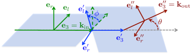
Figure 7: (Color online) RW: transformation of Stokes vectors. In the random walk model, a scattering event is determined by two consecutive transformations of local coordinates: $\{{\bf e}_{\rm 3},{\bf e}_{\rm r},{\bf e}_{\rm l}\}\rightarrow\{{\bf e}_{\rm 3}^{\prime},{\bf e}_{\rm r}^{\prime},{\bf e}_{\rm l}^{\prime}\}$ via rotation $\phi$, and $\{{\bf e}_{\rm 3}^{\prime},{\bf e}_{\rm r}^{\prime},{\bf e}_{\rm l}^{\prime}\}\rightarrow\{{\bf e}_{\rm 3}^{\prime\prime},{\bf e}_{\rm r}^{\prime\prime},{\bf e}_{\rm l}^{\prime\prime}\}$ via rotation $\theta$ Bartel and Hielscher (2000).

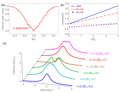
Figure 8: (Color online) RW Model. (a) Distribution of on-resonance intensity in the plane $\theta=\pi/2$. Along the direction where single scattering events are forbidden ($\phi=0$), the light intensity is suppressed. (b) The FWHM linewdith increases linearly with OD_p in a dilute medium. The linewidth along the direction parallel to the laser polarization can drop below $\Gamma$ for small (purple squares). (c) Lineshapes for different OD_ps and angles of observation. The lineshape is Lorentzian for low OD_p but gets distorted and develops a double-peak structure as the OD_p increases. Here, for all angles, the signal is collected within a small angular region $\delta\theta=5^{\circ}$. The intensity is normalized to the value at zero detuning for $\theta=0$ and OD_p=0.3, and the width of laser beam is 5 times the Gaussian width of the atomic cloud. Here all OD_p are labeled as the value at $\Delta=0$.

IV Role of atomic motion

An assumption made in Sec. II is that the position of the atoms remains fixed. This assumption is only valid when atoms move at a rate slower than the radiative decay rate. When motion is significantly faster, e.g. hot atomic clouds, the coherence during radiation is smeared out and classical approaches, such as the RW model, are usually satisfactory van Rossum and Nieuwenhuizen (1999); Brown and Mortensen (2000) to describe collective light emission. However, many experiments operate in an intermediate regime where coherences cannot be totally disregarded and it is not a good approximation to treat atoms as frozen. For example, for the ${}^{1}{\rm S}_{0}\rightarrow{}^{3}$P₁ transition of ⁸⁸Sr atoms, the Doppler boadening at $\sim 1~{}\mu$K, $\Delta_{\rm D}\approx 6\Gamma$, and recoil frequency $\omega_{r}=\hbar k_{0}^{2}/2m\approx 0.6\Gamma$, both comparable to the natural linewidth Ido et al. (2005); Trippenbach et al. (1992). Consequently for a proper description of light scattering one needs to account for both photon coherences and atomic motion on an equal footing. Below we present two approximate ways to accomplish this task:

IV.1 Modified frozen dipole model

In this section, we discuss a simple way to include the effects of atomic motion on light scattering via a modified CD model. Here we start by deriving the fluorescence intensity emitted by a weakly driven atom, using a full quantum approach with motional effect included. We consider the states including at most one excitation, and label the relevant quantum states by $\ket{{\bf p}\alpha,0},\ket{{\bf p}g,{\bf k}}$, with $\alpha=\{e,g\}$, p the momentum of the atom, and ${\bf k}$ is the momentum of the photon in vacuum ($\ket{{\bf p}\alpha,0}$ stands for no photon). For generality we assume here that two counter propagating lasers are used to drive the atoms, carrying momentum ${\bf k}_{0}$ and $-{\bf k}_{0}$ respectivelly. The Hamiltonian is fno (c)

$$\hat{H} = \frac{\hat{\bf p}^{2}}{2m}+\hbar\omega_{a}\hat{b}^{\dagger}\hat{b}+\hbar\Omega[{\rm cos}({\bf k}_{0}\cdot{\bf r})(e^{-i\omega_{L}t}\hat{b}^{\dagger}+\mathrm{H.c.})]$$

$$+\sum_{{\bf k},\bm{\epsilon}}\hbar\omega_{k}\hat{a}_{{\bf k}\bm{\epsilon}}^{\dagger}\hat{a}_{{\bf k},\bm{\epsilon}}-\hbar\sum_{{\bf k},\bm{\epsilon}}({\bf d}\cdot\hat{\bm{\epsilon}}_{\bf k})g_{k}[e^{i{\bf k}\cdot{\bf r}}\hat{a}_{{\bf k}\bm{\epsilon}}\hat{b}^{\dagger}+\mathrm{H.c.}].$$

The state vector of the system is

$$\ket{\psi} = \sum_{\alpha}\int d{\bf p}\ket{{\bf p}\alpha,0}A_{\alpha 0}({\bf p},t)e^{-i(E_{\alpha}+E_{p})t/\hbar}$$

$$+\sum_{{\bf k},\bm{\epsilon}}\int d{\bf p}\ket{{\bf p}g,{\bf k}}B_{g{\bf k}\bm{\epsilon}}({\bf p},t)e^{-i(E_{g}+E_{p}+\hbar\omega_{k})t/\hbar},$$

where $E_{\alpha}=\omega_{a}\delta_{\alpha,e}$, $E_{p}=\frac{p^{2}}{2m}$, $|A_{\alpha 0}({\bf p},t)|^{2}$ represents the population in the ground/excited state possessing momentum ${\bf p}$, and $B_{g{\bf k}\bm{\epsilon}}({\bf p},t)$ is the amplitude of having a photon ${\bf k}$ with polarization $\bm{\epsilon}$. The state of the system evolves according to

$$i\frac{dA_{g0}({\bf p},t)}{dt} = \Omega A_{e0}({\bf p}+{\bf k},t)e^{i(\omega_{L}-\omega_{a})t}e^{-iE_{{\bf p}+{\bf k}_{0},{\bf p}}t/\hbar}$$

$$+\Omega A_{e0}({\bf p}-{\bf k},t)e^{i(\omega_{L}-\omega_{a})t}e^{-iE_{{\bf p}-{\bf k}_{0},{\bf p}}t/\hbar},$$

$$i\frac{dA_{e0}({\bf p},t)}{dt} = -\sum_{{\bf k},\bm{\epsilon}}({\bf d}\cdot\hat{\bm{\epsilon}}_{\bf k})g_{k}B_{g{\bf k}\bm{\epsilon}}({\bf p}-{\bf k},t)$$

$$\times e^{-i(\omega_{k}-\omega_{a})t}e^{-iE_{{\bf p}-{\bf k},{\bf p}}t/\hbar}$$

$$+\Omega A_{g0}({\bf p}-{\bf k},t)e^{-i(\omega_{L}-\omega_{a})t}e^{-iE_{{\bf p}-{\bf k}_{0},{\bf p}}t/\hbar}$$

$$+\Omega A_{g0}({\bf p}+{\bf k},t)e^{-i(\omega_{L}-\omega_{a})t}e^{-iE_{{\bf p}+{\bf k}_{0},{\bf p}}t/\hbar},$$

$$i\frac{dB_{g{\bf k}\bm{\epsilon}}({\bf p},t)}{dt} = B_{g{\bf k}\bm{\epsilon}}({\bf p},t)-({\bf d}\cdot\hat{\bm{\epsilon}}_{\bf k})g_{k}A_{e0}({\bf p}+{\bf k},t)$$ (32)

$$\times e^{i(\omega_{k}-\omega_{a})t}e^{-iE_{{\bf p}+{\bf k},p}t/\hbar},$$

where $E_{p_{1},p_{2}}=\frac{p_{1}^{2}-p_{2}^{2}}{2m}$. The first term in Eq. (LABEL:eq:2nd) describes the effect of vacuum photons, which according to Wigner-Weisskopf approach leads to the spontaneous decay with rate $\Gamma$, and can be rewritten as Lam and Berman (1976)

$$i\frac{dA_{e0}({\bf p},t)}{dt} = -i\frac{\Gamma}{2}A_{e0}({\bf p},t)+\Omega A_{g0}({\bf p}-{\bf k},t)$$

$$\times e^{-i(\omega_{L}-\omega_{a})t}e^{-iE_{{\bf p}-{\bf k}_{0},{\bf p}}t/\hbar}$$

$$+\Omega A_{g0}({\bf p}+{\bf k},t)e^{-i(\omega_{L}-\omega_{a})t}e^{-iE_{{\bf p}+{\bf k}_{0},{\bf p}}t/\hbar}.$$

Consider the initial condition $B_{g{\bf k}\bm{\epsilon}}({\bf p},0)=0$, $A_{g0}=\delta({\bf p}-{\bf p}_{0})$, where ${\bf p}_{0}$ is the initial momentum of the atom. The steady state solution is

$$A_{e0}({\bf p},\infty)=\frac{\Omega[\delta({\bf p}_{0}-{\bf p}+{\bf k}_{0})+\delta({\bf p}_{0}-{\bf p}-{\bf k}_{0})]}{\Delta_{L}+E_{{\bf p}_{0},{\bf p}}+i\frac{\Gamma}{2}},$$

with $\Delta_{L}=\omega_{L}-\omega_{a}$. Thus the atomic excitation $\mathcal{A}_{e}=\int d{\bf p}|A_{e0}({\bf p},\infty)|^{2}$ indicates two Lorentzian with FWHM=$\Gamma$ and centered at $\omega_{r}\pm\frac{{\bf k}_{0}\cdot{\bf p}_{0}}{m}$. The photon emission rate along a given direction ${{\bf k}_{s}}$ is

$$I_{{\bf k}_{s}}=\frac{V\hbar c}{(2\pi)^{3}}\!\int\!dk~{}k^{3}\sum_{\bm{\epsilon}}\int\!d{\bf p}~{}\lim_{t\to\infty}\frac{|B_{g{\bf k}\bm{\epsilon}}({\bf p},t)|^{2}}{t},$$

with ${\bf k}=k\hat{\bf k}_{s}$. We consider the transverse intensity case where, ${\bf k}\cdot{\bf k}_{0}=0$, and for atomic transitions $\omega_{r},~{}{\bf p}_{0}\cdot{\bf k}_{0}/m\ll\omega_{L}$, then

$$I_{{\bf k}_{s}} \approx \frac{\omega_{L}^{4}}{c^{3}}\frac{d^{2}\Omega^{2}}{8\pi^{2}\varepsilon_{0}}[\frac{1}{(\Delta-\omega_{r}+\frac{{\bf k}_{0}\cdot{\bf p}_{0}}{m})^{2}+\frac{\Gamma^{2}}{4}}$$ (36)

$$+\frac{1}{(\Delta-\omega_{r}-\frac{{\bf k}_{0}\cdot{\bf p}_{0}}{m})^{2}+\frac{\Gamma^{2}}{4}}],$$

The emitted light intensity exhibits the same profile as the atomic excitation $\mathcal{A}_{e}$.

For a single atom, to leading order, motion modifies the emitted light intensity by adding two natural corrections: a Doppler shift $\propto\frac{{\bf k}_{0}\cdot{\bf p}_{0}}{m}$, a velocity dependent modification of the effective laser detuning experienced by an atom, and a recoil shift, $\omega_{r}$, which physically accounts for the fact that to compensate for the energy imparted to the atom via photon recoil, the incident laser needs to have a higher frequency to be resonant with the atomic transition.

We generalize the above results to deal with motional effects in the many-body system by introducing random detunings $\delta\nu$ for each atom, and by sampling them according to a Maxwell-Boltzmann distribution $P(\delta\nu)=\frac{1}{\sqrt{2\pi}\widetilde{\Delta}_{\rm D}}{\rm exp}\left(-\frac{\delta\nu^{2}}{2\widetilde{\Delta}_{\rm D}^{2}}\right)$ that accounts for the Doppler shifts Javanainen et al. (2014). Here $\widetilde{\Delta}_{\rm D}=\Delta_{\rm D}/\sqrt{8{\rm ln}2}$. We denote this approximation as the modified frozen dipole model. The random detunings have two straightforward effects: (i) dephasing and (ii) reduced light scattering probability Bromley et al. (2016). (i) Dephasing reduces the forward enhancement of fluorescence intensity as shown in Fig. 9 (a). This can be understood even at the level of non-interacting two-level atoms, where Doppler shifts modify atomic coherences as (for simplicity we assume a single beam illumination):

$$b_{j} = \frac{\Omega e^{i{\bf k}_{0}\cdot{\bf r}_{j}}}{(\Delta-\delta\nu_{j})+i\Gamma/2}.$$ (37)

Using Eq. (37), the intensity along a generic direction becomes

$$I_{\rm incoh} = \frac{1}{\sqrt{2\pi}\widetilde{\Delta}_{\rm D}}\int d\delta\nu_{j}|b_{j}|^{2}e^{-\delta\nu_{j}^{2}/2\widetilde{\Delta}_{\rm D}^{2}}.$$ (38)

On the other hand, the coherent scattering in the forward direction which takes into account pairwise atomic contributions, becomes

$$I_{\rm coh}\! = \!\frac{1}{2\pi\widetilde{\Delta}_{\rm D}^{2}}\!\!\int\!\!d\delta\nu_{j}d\delta\nu_{j^{\prime}}b_{j}b^{*}_{j^{\prime}}e^{-\delta\nu_{j}^{2}/2\widetilde{\Delta}_{\rm D}^{2}}e^{-\delta\nu_{j^{\prime}}^{2}/2\widetilde{\Delta}_{\rm D}^{2}}.$$ (39)

The on-resonance enhancement factor is thus

$$\frac{I_{\rm coh}}{I_{\rm incoh}} = \frac{\sqrt{\frac{\pi}{2}}e^{\frac{1}{8\widetilde{\Delta}_{\rm D}^{2}/\Gamma^{2}}}{\rm Erfc}(\frac{1}{2\sqrt{2}\widetilde{\Delta}_{\rm D}/\Gamma})}{2\widetilde{\Delta}_{\rm D}/\Gamma},$$ (40)

where ${\rm Erfc}$ is the complementary error function. This shows an exponential suppression of the forward interference that depends on $\widetilde{\Delta}_{\rm D}/\Gamma$.

The reduced light scattering probability, on the other hand, competes with dephasing since it suppresses multiple scattering, and as a consequence promotes collective enhancement. Effectively, it brings the system closer to the small OD regime (Fig. 2(b)). The motion induced suppression of multi-scattering processes is also signaled in the frequency shift (Fig. 4) Javanainen et al. (2014); Jenkins et al. (2016), which keeps increasing until a larger value of density in the presence of motion.

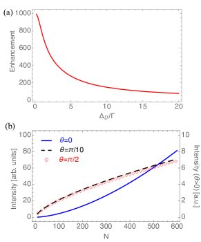
Figure 9: (Color online) Modified frozen dipole model: peak intensity. (a) Collective forward enhancement: forward intensity normalized by the transverse intensity as a function of Doppler width. (b) Intensity detected along different directions at Doppler width $\Delta_{\rm D}=6\Gamma$ as a function of atom number for fixed cloud size (when $N=500$, OD=2,$n_{0}k_{0}^{-3}$=0.0015). $I\sim N^{1.6}$ for $\theta=0$, and $I\sim N^{0.7}$ for $\theta=\pi/2$. The right vertical axis labels the intensity for $\theta=\pi/2,\pi/10$.

IV.2 Semi-classical approach

Laser light mediated forces on atoms are a fundamental concept in atomic physics and lay the foundations of laser trapping and cooling Phillips (1998). They can be accounted for at the semiclassical level by explicitly including the position ${\bf r}_{i}$ and the momentum ${\bf p}_{i}$ degrees of freedom of the atoms, and solving for their dynamics while feeding those back into the quantum dynamics of the internal degrees of freedom. An explicit description of this procedure is presented below.

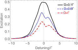
Figure 10: (Color online) Semi-classical model: single-atom lineshape. The excitation lineshape is calculated for three different driving strength, each normalized by $\Omega^{2}$. The atomic motion is allowed to be one-dimensional and parallel to the laser propagating direction. Here we used $\omega_{r}=0.6\Gamma$ (the value of the ${}^{1}{\rm S}_{0}\rightarrow{}^{3}$P₁ transition of Sr Ido et al. (2005)).

For simplicity we will assume a two-level transition, with $\omega_{a}=k_{0}c$ the frequency of transition and ${\bf d}$ the dipole moment. This condition is achievable in experiments, for example, by applying a large magnetic field to split apart ($|\Delta^{\alpha}-\Delta^{\gamma}|\gg{\mathcal{G}}\Gamma$) the excited state levels and thus energetically suppressing population of the ones not directly driven by the laser.

Let us first ignore the driving term and include motion in the dipolar coupling after eliminating the electromagnetic vacuum modes. The Hamiltonian, including the atoms and free-space electromagnetic field is

$$H = \hbar\omega_{a}\sum_{j}\hat{b}_{j}^{\dagger}\hat{b}_{j}+\sum_{{\bf k},\bm{\epsilon}}\omega_{k}\hat{a}^{\dagger}_{{\bf k}\bm{\epsilon}}\hat{a}_{{\bf k}\bm{\epsilon}}-\sum_{j}\sum_{{\bf k},\bm{\epsilon}}g_{k}$$ (41)

$$\times({\bf d}\cdot\hat{\bm{\epsilon}}_{\bf k})[(e^{i{\bf k}\cdot{\bf r}_{j}}\hat{a}_{{\bf k}\bm{\epsilon}}+\mathrm{H.c.})(\hat{b}_{j}^{\dagger}+\mathrm{H.c.})].$$

The evolution of atomic dipoles and the field modes are

$$\frac{d\hat{a}_{{\bf k}\bm{\epsilon}}}{dt} = -i\omega_{k}\hat{a}_{{\bf k}\bm{\epsilon}}+\frac{i}{\hbar}\sum_{j}g_{k}({\bf d}_{j}\cdot\bm{\epsilon}_{\bf k})[e^{-i{\bf k}\cdot{\bf r}_{j}}(\hat{b}_{j}+\mathrm{H.c.})],$$

$$\frac{d\hat{b}_{j}}{dt} = -i\omega_{a}\hat{b}_{j}+i\sum_{{\bf k},\bm{\epsilon}}\frac{g_{k}}{\hbar}({\bf d}_{j}\cdot\hat{\bm{\epsilon}}_{\bf k})[e^{i{\bf k}\cdot{\bf r}_{j}}\hat{a}_{{\bf k}\bm{\epsilon}}\hat{s}_{j}+\mathrm{H.c.}],$$

$$\frac{d\hat{s}_{j}}{dt} = -i\sum_{{\bf k},\bm{\epsilon}}\frac{g_{k}}{\hbar}({\bf d}_{j}\cdot\hat{\bm{\epsilon}}_{\bf k})[e^{i{\bf k}\cdot{\bf r}_{j}}\hat{a}_{{\bf k}\bm{\epsilon}}\hat{b}_{j}^{\dagger}-e^{-i{\bf k}\cdot{\bf r}_{j}}\hat{a}_{{\bf k}\bm{\epsilon}}^{\dagger}\hat{b}_{j}$$ (44)

$$-e^{i{\bf k}\cdot{\bf r}_{j}}\hat{a}_{{\bf k}\bm{\epsilon}}\hat{b}_{j}+e^{-i{\bf k}\cdot{\bf r}_{j}}\hat{a}_{{\bf k}\bm{\epsilon}}^{\dagger}\hat{b}_{j}^{\dagger}],$$

where $\hat{s}_{j}=\hat{b}_{j}^{\dagger}\hat{b}_{j}-\hat{b}_{j}\hat{b}_{j}^{\dagger}$, and $s_{j}=\langle\hat{s}_{j}\rangle$ gives the inversion of the $j^{\rm th}$ atom. We have assumed that internal operators commute with external operators, and neglected the diffusion of the atomic wavepacket. Eq. (IV.2) can be formally integrated to obtain

$$\hat{a}_{{\bf k}\bm{\epsilon}}(t) = \hat{a}_{{\bf k}\bm{\epsilon}}(0)-i\sum_{j}\frac{g_{k}}{\hbar}({\bf d}_{j}\cdot\hat{\bm{\epsilon}}_{\bf k})\int dt^{\prime}~{}e^{i{\bf k}\cdot{\bf r}_{j}+i\omega_{k}(t^{\prime}-t)}$$ (45)

$$\times(\hat{b}_{j}+\mathrm{H.c.}),$$

in which we have assumed the external motion is much slower than the internal dynamics so that ${\bf r}_{j}(t^{\prime})\approx{\bf r}_{j}(t)$, and the interaction between atoms and the field modes is weak so that $\hat{b}_{j}(t^{\prime})\approx\hat{b}_{j}(t)e^{-i\omega_{a}(t^{\prime}-t)}$. Substituting Eq. (45) into Eq. (IV.2), we obtain the equation for the quantum averaged quantities

$$\frac{db_{j}}{dt} = -i\omega_{a}b_{j}+s_{j}\sum_{l}\sum_{{\bf k},\bm{\epsilon}}\frac{g_{k}^{2}}{\hbar^{2}}({\bf d}_{j}\cdot\hat{\bm{\epsilon}}_{\bf k})({\bf d}_{l}\cdot\hat{\bm{\epsilon}}_{\bf k})$$ (46)

$$\times\{e^{i{\bf k}\cdot{\bf r}_{jl}}[b_{l}^{*}(\pi\delta(\omega_{k}+\omega_{a})-i{\rm P}\frac{1}{\omega_{k}+\omega_{a}})$$

$$+b_{l}(\pi\delta(\omega_{k}-\omega_{a})-i{\rm P}\frac{1}{\omega_{k}-\omega_{a}})]$$

$$-e^{-i{\bf k}\cdot{\bf r}_{jl}}[b_{l}^{*}(\pi\delta(\omega_{k}-\omega_{a})+i{\rm P}\frac{1}{\omega_{k}-\omega_{a}})$$

$$+b_{l}(\pi\delta(\omega_{k}+\omega_{a})+i{\rm P}\frac{1}{\omega_{k}+\omega_{a}})]\},$$

where $\mathcal{O}=\langle\hat{\mathcal{O}}\rangle$ for any atomic operator $\hat{\mathcal{O}}$, and we have utilized the fact that $\langle\hat{a}_{{\bf k}\bm{\epsilon}}(0)\rangle=0$, and assumed that atomic motion is classical Smith and Burnett (1991, 1992). Changing $\sum_{\bf k}=\frac{V}{(2\pi)^{3}}\int d\Omega\,dk~{}k^{2}$, and applying rotating wave approximation, we have

$$\frac{db_{j}}{dt} = -i\omega_{a}b_{j}+i\sum_{l\neq j}s_{j}b_{l}(g_{jl}-if_{jl})-\frac{\Gamma}{2}b_{j},$$ (47)

with $f(0)=\Gamma$. The equation for $s_{j}$ can be derived in a similar way and is given by

$$\frac{ds_{j}}{dt} = -\Gamma s_{j}-2i\sum_{l\neq j}(g_{jl}-if_{jl})b_{j}^{*}b_{l}+2i\sum_{l\neq j}(g_{jl}+if_{jl})b_{l}^{*}b_{j},$$

and

$$g(r) = -\frac{3\Gamma}{4}(z_{1}(\theta)\frac{{\rm cos}k_{0}r}{k_{0}r}+z_{2}(\theta)[\frac{{\rm cos}k_{0}r}{k_{0}^{3}r^{3}}+\frac{{\rm sin}k_{0}r}{k_{0}^{2}r^{2}}]),$$

$$f(r) = \frac{3\Gamma}{4}(z_{1}(\theta)\frac{{\rm sin}k_{0}r}{k_{0}r}+z_{2}(\theta)[\frac{{\rm sin}k_{0}r}{k_{0}^{3}r^{3}}\!-\!\frac{{\rm cos}k_{0}r}{k_{0}^{2}r^{2}}]),$$ (50)

where $z_{1}(\theta)={\rm sin}^{2}\theta$, and $z_{2}(\theta)=(3{\rm cos}^{2}\theta-1)$. For the momentum,

$$\frac{d\hat{\bf p}_{j}}{dt} = -\nabla\hat{H}$$ (51)

$$= -\sum_{{\bf k},\bm{\epsilon}}g_{k}({\bf d}_{j}\cdot\bm{\epsilon}_{\bf k})(i{\bf k}e^{i{\bf k}\cdot{\bf r}_{j}}\hat{a}_{{\bf k}\bm{\epsilon}}\hat{b}_{j}^{\dagger}-i{\bf k}e^{-i{\bf k}\cdot{\bf r}_{j}}\hat{a}_{{\bf k}\bm{\epsilon}}^{\dagger}\hat{b}_{j}$$

$$+i{\bf k}e^{i{\bf k}\cdot{\bf r}_{j}}\hat{a}_{{\bf k}\bm{\epsilon}}\hat{b}_{j}-i{\bf k}e^{-i{\bf k}\cdot{\bf r}_{j}}\hat{a}_{{\bf k}\bm{\epsilon}}^{\dagger}\hat{b}_{j}^{\dagger}).$$

After substituting Eq. (45), taking the quantum average and performing a similar integration procedure of as above, we obtain

$$\frac{d{\bf p}_{j}}{dt} = \sum_{l\neq j}[\mathpzc{g}_{jl}(b_{j}b_{l}^{*}+\mathrm{H.c.})-i\mathpzc{f}_{jl}(b_{j}b_{l}^{*}-\mathrm{H.c.})],$$ (52)

with $\mathpzc{g}_{jl}=-\nabla g_{jl}$ and $\mathpzc{f}_{jl}=-\nabla f_{jl}$. As the dispersive force $\mathpzc{g}_{jl}$ is a steep function of $r_{jl}$, it dominates at short distance, and atoms are drastically accelerated/decelerated. Both the dispersive and dissipative forces are anisotropic and couple motion along different directions.

The prior equations of motion however are not the full story. Due to the presence of spontaneous emission and radiative interactions, the atomic momentum diffuses over time, which can be described by including classical noise $d\xi_{i}^{\alpha}$ in the equation of motion for $p_{i}^{\alpha}$. The components of these noises are correlated, and characterized by the diffusion matrix

$$E[d\xi_{i}^{\alpha}(t)d\xi_{i}^{\beta}(t^{\prime})] = \delta_{\alpha,\beta}\frac{2-\delta_{\alpha,z}}{20}\hbar^{2}k_{0}^{2}\Gamma(s_{i}+1)\delta(t-t^{\prime}),$$

$$E[d\xi_{i}^{\alpha}(t)d\xi_{j}^{\beta}(t^{\prime})] = -\hbar^{2}k_{0}^{2}\nabla_{\alpha}\nabla_{\beta}f(r_{ij})\Re[b^{*}_{i}b_{j}]\delta(t-t^{\prime}),$$

where $E[\cdot]$ denotes the expectation value.

The momentum diffusion matrix can be found from

$$\mathcal{D}_{jl} = \frac{d\langle\hat{\bf p}_{j}\hat{\bf p}_{l}\rangle}{dt}-\langle{\bf p}_{j}\rangle\frac{d\langle{\bf p}_{l}\rangle}{dt}-\frac{d\langle{\bf p}_{j}\rangle}{dt}\langle{\bf p}_{l}\rangle$$

$$= \sum_{{\bf k}_{1},\bm{\epsilon_{1}}}\sum_{{\bf k}_{2},\bm{\epsilon}_{2}}g_{k_{1}}g_{k_{2}}({\bf d}_{j}\cdot\bm{\epsilon}_{1})({\bf d}_{l}\cdot\bm{\epsilon}_{2})(i{\bf k}_{1}e^{i{\bf k}_{1}\cdot{\bf r}_{j}}\hat{a}_{{\bf k}_{1}\bm{\epsilon}_{1}}\hat{b}_{j}^{\dagger}$$

$$-i{\bf k}_{1}e^{-i{\bf k}_{1}\cdot{\bf r}_{j}}\hat{a}_{{\bf k}_{1}\bm{\epsilon}_{1}}^{\dagger}\hat{b}_{j}$$

$$+i{\bf k}_{1}e^{i{\bf k}_{1}\cdot{\bf r}_{j}}\hat{a}_{{\bf k}_{1}\bm{\epsilon}_{1}}\hat{b}_{j}-i{\bf k}_{1}e^{-i{\bf k}_{1}\cdot{\bf r}_{j}}\hat{a}_{{\bf k}_{1}\bm{\epsilon}_{1}}^{\dagger}\hat{b}_{j}^{\dagger})$$

$$\times(i{\bf k}_{2}e^{i{\bf k}_{2}\cdot{\bf r}_{l}}\hat{a}_{{\bf k}_{2}\bm{\epsilon}_{2}}\hat{b}_{l}^{\dagger}-i{\bf k}_{2}e^{-i{\bf k}_{2}\cdot{\bf r}_{l}}\hat{a}_{{\bf k}_{2}\bm{\epsilon}_{2}}^{\dagger}\hat{b}_{l}$$

$$+i{\bf k}_{2}e^{i{\bf k}_{2}\cdot{\bf r}_{l}}\hat{a}_{{\bf k}_{2}\bm{\epsilon}_{2}}\hat{b}_{l}-i{\bf k}_{2}e^{-i{\bf k}_{2}\cdot{\bf r}_{l}}\hat{a}_{{\bf k}_{2}\bm{\epsilon}_{2}}^{\dagger}\hat{b}_{l}^{\dagger})$$

$$= -\hbar^{2}k_{0}^{2}\nabla\nabla f_{ij}\Re[b_{j}^{*}b_{l}].$$ (56)

In dense clouds momentum diffusion from radiative interactions can give rise at long times to significant heating. This heating was reported to be one of the main limiting mechanisms in laser cooling Castin et al. (1989); Smith and Burnett (1992). At short times, $t\Gamma\sim 1$, with low densities and weak probes, $\Omega<\Gamma$, the momentum diffusion is not prominent, and since this is the regime we are interested in this work, we will ignore momentum diffusion in our calculations.

For driving the atoms we will consider the case of two counter-propagating lasers with wavevector $\pm{\bf k}_{0}$, propagating along $z$. The laser generates an additional force $-2\hbar{\bf k}_{0}\Omega{\rm sin}({\bf k}_{0}\cdot{\bf r}_{i})\Re\{b_{i}(t)\}$ and drives the laser coherences as $\frac{db_{i}}{dt}=i\Omega\cos({\bf k}_{0}\cdot{\bf r}_{i})s_{i}$ Chabé et al. (2014). Those terms need to be added in the corresponding equations.

From previous sections, it has been shown that except for a narrow cone around the forward direction, the fluorescence intensity is $I({\bf r}_{s})\propto\sum_{i}s_{i}$. Since we expect motion to further reduce the effect of coherence, we will focus on the transverse scattering, and compute $\sum_{i}s_{i}$. Fig. 10 shows the lineshape of a single atom for different $\Omega$ calculated from the semi-classical approach, without accounting for momentum diffusion. We have verified in our numerical simulations that it can be safely ignored for most of the parameters presented there.

As a result of atomic motion, the laser-atom system is not in a stationary state. We show the results for driving time $t=5/\Gamma$. When $\Omega\ll\Gamma$, the lineshape is a Voigt profile with the Doppler width determined by the velocity. When $\Omega\sim\Gamma$, there is a distortion in the lineshape, with more intensity at $\Delta<0$. This is because for $\Delta<0$ the laser force decelerates the atom, while for $\Delta>0$ the atom is heated up. With reduced/increased velocity, the atom is on average more/less excited, resulting in a distorted lineshape. The center of the line is therefore shifted to the red.

Motion can significantly modify the interactions between atoms Damanet et al. (2016). We study the effect of motion on the frequency shift in Fig. 11. Dipolar induced frequency shifts were previously discussed in Sec. II. Since we focus on low driving fields, again we neglect momentum diffusion in these calculations. The calculations show that unless $\Delta_{\rm D}$ is very small, atomic motion leads to a fast suppression of the frequency shift. Only when $\Delta_{\rm D}\ll\Gamma$, the frequency can be increased by motion and this is the regime where the modified frozen dipole model is qualitatively valid; recall, it predicts always an increase of density shift with Doppler broadening. We note that at $\Delta_{\rm D}\rightarrow 0$ the frequency shift obtained using the modified frozen dipole model, is slightly smaller than that one obtained from the semi-classical approach. This is a consequence of the distortion caused by laser cooling/heating which additionally shifts the spectral line. For $\Delta_{\rm D}\gtrsim\Gamma$ motion needs to be properly accounted for and the modified frozen dipole model is not reliable.

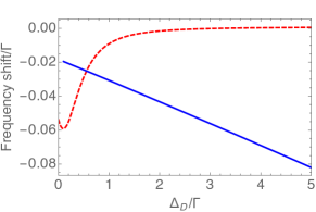
Figure 11: (Color online) Semi-classical model: effect of motion on frequency shift. Two atoms are driven by a pair of counter-propagating lasers, with $\Omega=0.1\Gamma$, $\omega_{r}=0.6\Gamma$. The red dashed line shows the result of semi-classical model where motion is allowed in three dimensions. The blue line shows the result from the modified CD. The center of excitation lineshape is calculated at $t=5/\Gamma$ for different Doppler width, for both models.

V Conclusion

We theoretically studied the propagation of light through a cold atomic medium. We presented two different microscopic models, the “coherent dipole model” and the “random walk model”, and analyzed how the light polarization, optical depth and density affect the linewidth broadening, intensity and line center shift of the emitted light. We showed that the random walk model, which neglects photonic phase coherence, can fairly capture the collective broadening (narrowing) of the emission linewidth but on the other hand does not predict a density shift. Due to the limitation of computation capacity, the numerical simulation of CD is usually restricted to $\sim 10^{4}$ atoms, which is much smaller than that in some cold atom experiments Guerin et al. (2016); Balik et al. (2013). Nevertheless, the understanding of the underlying physics allowed us to perform an appropriate rescaling in the cloud size which we used to compare with experiments Bromley et al. (2016). We further developed generalized models that explicitly take into account motional effects. We showed that atomic motion can lead to drastic dephasing and reduction in the collective effects, together with a distortion in the lineshape. While the modified frozen dipole model predicts a monotonic increase of the density shift with increasing motion, the semiclassical model, which properly accounts for recoil effects, predicts that this behavior only holds at slow motion $\Delta_{\rm D}\ll\Gamma$. Instead, as atoms move faster, motional effects start to become dominant, the cloud expands and the frequency shift decreases. None of the presented theoretical models, however, can explain the large density shift measured in the ${}^{1}{\rm S}_{0}\rightarrow{}^{3}{\rm P}_{1}$ transition of ⁸⁸Sr atoms Ido et al. (2005). It will be intriguing to determine what are the actual physical processes that cause this large shift.

VI Acknowledgements

The authors wish to acknowledge useful discussions with JILA Ye group, Alexey Gorshkov, Juha Javanainen, Mark Havey, Muray Holland, Michael L. Wall, Jose D’Incao, Matthew Davis, and Johannes Schachenmayer. We would like to especially thank Robin Kaiser for helpful discussions and insightful comments. This work was supported by the NSF (PIF-1211914 and PFC-1125844), AFOSR, AFOSR-MURI, NIST and ARO. Computations utilized the Janus supercomputer, supported by NSF (award number CNS-0821794), NCAR, and CU Boulder/Denver.

Appendix A Optical depth of a cloud with Gaussian distribution

We consider an atomic cloud with a Gaussian distribution $n(x,y,z)=n_{0}e^{-\frac{x^{2}}{2R_{x}^{2}}-\frac{y^{2}}{2R_{y}^{2}}-\frac{z^{2}}{2R_{z}^{2}}}$, where $n_{0}$ satisfies $\int dxdydz\,n(x,y,z)=N$, and $N$ is the total number of atoms. Along the line of observation, e.g. $\hat{x}$, the on resonance optical depth is related to the resonant scattering cross section, which for the $J=0\rightarrow J=1$ transition is $\sigma_{sc}=\sigma_{0}(\Delta=0)=\frac{6\pi}{k_{0}^{2}}$, and the column density averaged over the profile perpendicular to this direction Chomaz et al. (2012); Bienaimé et al. (2012),

$${\rm OD} = [\int dydz\,n(y,z)]^{-1}\int dydz\,n(y,z){\rm OD}(y,z)$$ (57)

$$= [\int dydz\,n(y,z)]^{-1}\int dydz\,n(y,z)\int dxn(x,y,z)\sigma_{sc}$$

$$= [\int dydz\,n(y,z)]^{-1}dydz\,n(y,z)e^{-\frac{y^{2}}{2R_{y}^{2}}-\frac{z^{2}}{2R_{z}^{2}}}$$

$$\times\int dx\,n_{0}e^{-\frac{x^{2}}{2R_{x}^{2}}}\sigma_{sc}$$

$$= \frac{3N}{2k_{0}^{2}R_{y}R_{z}}$$

$$= \frac{3N}{2k_{0}^{2}R_{\perp}^{2}}.$$

With laser detuning $\Delta$, the optical depth is ${\rm OD}/(1+4\Delta^{2}/\Gamma^{2})$.

References

- Kimble (2008) H. J. Kimble, Nature 453, 1023 (2008).
- Cirac et al. (1997) J. I. Cirac, P. Zoller, H. J. Kimble, and H. Mabuchi, Phys. Rev. Lett. 78, 3221 (1997).
- De Riedmatten et al. (2008) H. De Riedmatten, M. Afzelius, M. U. Staudt, C. Simon, and N. Gisin, Nature 456, 773 (2008).
- Douglas et al. (2015) J. S. Douglas, H. Habibian, C.-L. Hung, A. Gorshkov, H. J. Kimble, and D. E. Chang, Nature Photonics 9, 326 (2015).
- Bloch (2005) I. Bloch, Nature Physics 1, 23 (2005).
- Jotzu et al. (2014) G. Jotzu, M. Messer, R. Desbuquois, M. Lebrat, T. Uehlinger, D. Greif, and T. Esslinger, Nature 515, 237 (2014).
- Bloch et al. (2012) I. Bloch, J. Dalibard, and S. Nascimbène, Nature Physics 8, 267 (2012).
- Bohnet et al. (2012) J. G. Bohnet, Z. Chen, J. M. Weiner, D. Meiser, M. J. Holland, and J. K. Thompson, Nature 484, 78 (2012).
- Guerin et al. (2016) W. Guerin, M. O. Araújo, and R. Kaiser, Phys. Rev. Lett. 116, 083601 (2016).
- Safavi-Naeini et al. (2011) A. H. Safavi-Naeini, T. M. Alegre, J. Chan, M. Eichenfield, M. Winger, Q. Lin, J. T. Hill, D. Chang, and O. Painter, Nature 472, 69 (2011).
- Ourjoumtsev et al. (2011) A. Ourjoumtsev, A. Kubanek, M. Koch, C. Sames, P. W. Pinkse, G. Rempe, and K. Murr, Nature 474, 623 (2011).
- Brooks et al. (2012) D. W. Brooks, T. Botter, S. Schreppler, T. P. Purdy, N. Brahms, and D. M. Stamper-Kurn, Nature 488, 476 (2012).
- James (1993) D. F. V. James, Phys. Rev. A 47, 1336 (1993).
- Lehmberg (1970) R. H. Lehmberg, Phys. Rev. A 2, 883 (1970).
- Ruostekoski and Javanainen (1997) J. Ruostekoski and J. Javanainen, Phys. Rev. A 55, 513 (1997).
- Javanainen et al. (1999) J. Javanainen, J. Ruostekoski, B. Vestergaard, and M. R. Francis, Phys. Rev. A 59, 649 (1999).
- Scully et al. (2006) M. O. Scully, E. S. Fry, C. H. R. Ooi, and K. Wódkiewicz, Phys. Rev. Lett. 96, 010501 (2006).
- Svidzinsky et al. (2010) A. A. Svidzinsky, J.-T. Chang, and M. O. Scully, Phys. Rev. A 81, 053821 (2010).
- Bienaimé et al. (2012) T. Bienaimé, N. Piovella, and R. Kaiser, Phys. Rev. Lett. 108, 123602 (2012).
- Sokolov et al. (2013) I. Sokolov, A. Kuraptsev, D. Kupriyanov, M. Havey, and S. Balik, Journal of Modern Optics 60, 50 (2013).
- Javanainen et al. (2014) J. Javanainen, J. Ruostekoski, Y. Li, and S.-M. Yoo, Phys. Rev. Lett. 112, 113603 (2014).
- Sokolov (2015) I. Sokolov, Laser Physics 25, 065202 (2015).
- Olave et al. (2015) R. Olave, A. Win, K. Kemp, S. Roof, S. Balik, M. Havey, I. Sokolov, and D. Kupriyanov, From Atomic to Mesoscale: The Role of Quantum Coherence in Systems of Various Complexities. Edited by Malinovskaya Svetlana A et al. Published by World Scientific Publishing Co. Pte. Ltd., 2015. ISBN# 9789814678704, pp. 39-59 1, 39 (2015).
- Jennewein et al. (2015a) S. Jennewein, M. Besbes, N. Schilder, S. Jenkins, C. Sauvan, J. Ruostekoski, J.-J. Greffet, Y. Sortais, and A. Browaeys, arXiv preprint arXiv:1510.08041 (2015a).
- Javanainen and Ruostekoski (2016) J. Javanainen and J. Ruostekoski, Optics Express 24, 993 (2016).
- Jenkins et al. (2016) S. Jenkins, J. Ruostekoski, J. Javanainen, R. Bourgain, S. Jennewein, Y. Sortais, and A. Browaeys, arXiv preprint arXiv:1602.01037 (2016).
- Araújo et al. (2016) M. O. Araújo, I. Kresic, R. Kaiser, and W. Guerin, arXiv preprint arXiv:1603.07204 (2016).
- Olmos et al. (2013) B. Olmos, D. Yu, Y. Singh, F. Schreck, K. Bongs, and I. Lesanovsky, Phys. Rev. Lett. 110, 143602 (2013).
- Maier et al. (2014) T. Maier, S. Kraemer, L. Ostermann, and H. Ritsch, Opt. Express 22, 13269 (2014).
- Yu (2015) D. Yu, Journal of Modern Optics pp. 1–15 (2015).
- Zhu et al. (2015) B. Zhu, J. Schachenmayer, M. Xu, F. Herrera, J. G. Restrepo, M. J. Holland, and A. M. Rey, New Journal of Physics 17, 083063 (2015).
- Bettles et al. (2015) R. J. Bettles, S. A. Gardiner, and C. S. Adams, Physical Review A 92, 063822 (2015).
- Berman (1997) P. R. Berman, Phys. Rev. A 55, 4466 (1997).
- Li et al. (2013) Q. Li, D. Xu, C. Cai, and C. Sun, Scientific reports 3 (2013).
- Jennewein et al. (2015b) S. Jennewein, Y. Sortais, J.-J. Greffet, and A. Browaeys, arXiv preprint arXiv:1511.08527 (2015b).
- Goldschmidt et al. (2015) E. Goldschmidt, T. Boulier, R. Brown, S. Koller, J. Young, A. Gorshkov, S. Rolston, and J. Porto, arXiv preprint arXiv:1510.08710 (2015).
- de Vries et al. (1998) P. de Vries, D. V. van Coevorden, and A. Lagendijk, Rev. Mod. Phys. 70, 447 (1998).
- van Rossum and Nieuwenhuizen (1999) M. C. W. van Rossum and T. M. Nieuwenhuizen, Rev. Mod. Phys. 71, 313 (1999).
- Labeyrie et al. (2003) G. Labeyrie, D. Delande, C. A. Müller, C. Miniatura, and R. Kaiser, Phys. Rev. A 67, 033814 (2003).
- Brown and Mortensen (2000) W. Brown and K. Mortensen, Scattering in Polymeric and Colloidal Systems (Taylor & Francis, 2000), ISBN 9789056992606.
- Labeyrie et al. (1999) G. Labeyrie, F. de Tomasi, J.-C. Bernard, C. A. Müller, C. Miniatura, and R. Kaiser, Phys. Rev. Lett. 83, 5266 (1999).
- Labeyrie et al. (2004a) G. Labeyrie, D. Delande, C. A. Mueller, C. Miniatura, and R. Kaiser, Optics communications 243, 157 (2004a).
- Sigwarth et al. (2004) O. Sigwarth, G. Labeyrie, T. Jonckheere, D. Delande, R. Kaiser, and C. Miniatura, Phys. Rev. Lett. 93, 143906 (2004).
- Labeyrie et al. (2006) G. Labeyrie, D. Delande, R. Kaiser, and C. Miniatura, Phys. Rev. Lett. 97, 013004 (2006).
- Chomaz et al. (2012) L. Chomaz, L. Corman, T. Yefsah, R. Desbuquois, and J. Dalibard, New Journal of Physics 14, 055001 (2012).
- Yu (2014) D. Yu, Phys. Rev. A 89, 063809 (2014).
- Bienaimé et al. (2014) T. Bienaimé, R. Bachelard, J. Chabé, M. Rouabah, L. Bellando, P. Courteille, N. Piovella, and R. Kaiser, Journal of Modern Optics 61, 18 (2014).
- Sutherland and Robicheaux (2016) R. T. Sutherland and F. Robicheaux, Phys. Rev. A 93, 023407 (2016).
- Miroshnychenko et al. (2013) Y. Miroshnychenko, U. V. Poulsen, and K. Mølmer, Phys. Rev. A 87, 023821 (2013).
- Meir et al. (2014) Z. Meir, O. Schwartz, E. Shahmoon, D. Oron, and R. Ozeri, Phys. Rev. Lett. 113, 193002 (2014).
- Bromley et al. (2016) S. L. Bromley, B. Zhu, M. Bishof, X. Zhang, T. Bothwell, J. Schachenmayer, T. L. Nicholson, R. Kaiser, S. F. Yelin, M. D. Lukin, et al., Nature communications 7, 11039 (2016).
- Roof et al. (2016) S. Roof, K. Kemp, M. Havey, and I. Sokolov, arXiv preprint arXiv:1603.07268 (2016).
- Gross and Haroche (1982) M. Gross and S. Haroche, Physics Reports 93, 302 (1982).
- Friedberg et al. (1972) R. Friedberg, S. Hartmann, and J. Manassah, Physics Letters A 40, 365 (1972), ISSN 0375-9601.
- fno (a) Note: Around the direction there is a small enhancement due to the coherent backward scattering Labeyrie et al. (2003).
- Lagendijk and Van Tiggelen (1996) A. Lagendijk and B. A. Van Tiggelen, Physics Reports 270, 143 (1996).
- Friedberg et al. (1973) R. Friedberg, S. Hartmann, and J. Manassah, Physics Reports 7, 101 (1973), ISSN 0370-1573.
- Balik et al. (2013) S. Balik, A. L. Win, M. D. Havey, I. M. Sokolov, and D. V. Kupriyanov, Phys. Rev. A 87, 053817 (2013).
- Labeyrie et al. (2004b) G. Labeyrie, D. Delande, C. Müller, C. Miniatura, and R. Kaiser, Optics Communications 243, 157 (2004b), ISSN 0030-4018, ultra Cold Atoms and Degenerate Quantum Gases.
- fno (b) Note: For a cloud with a Gaussian distribution, the size of the incident laser beam needs to be taken into account, since a broad beam experiences fewer scattering events at the edge of the cloud and the actual optical depth depends on the transverse coordinates. The finite beamsize is not taken into account in the CD presented here. In RW we choose the beamsize to be 5 times the Gaussian width of the cloud.
- Chabé et al. (2014) J. Chabé, M.-T. Rouabah, L. Bellando, T. Bienaimé, N. Piovella, R. Bachelard, and R. Kaiser, Phys. Rev. A 89, 043833 (2014).
- Raković et al. (1999) M. J. Raković, G. W. Kattawar, M. Mehrűbeoğlu, B. D. Cameron, L. V. Wang, S. Rastegar, and G. L. Coté, Appl. Opt. 38, 3399 (1999).
- Hovenier et al. (2004) J. Hovenier, C. Mee, and H. Domke, Transfer of Polarized Light in Planetary Atmospheres: Basic Concepts and Practical Methods, Astrophysics and Space Science Library (Springer, 2004), ISBN 9781402028557.
- Brosseau (1998) C. Brosseau, Fundamentals of polarized light: a statistical optics approach, Wiley-interscience publication (John Wiley, 1998), ISBN 9780471143024.
- Bartel and Hielscher (2000) S. Bartel and A. H. Hielscher, Appl. Opt. 39, 1580 (2000).
- Ido et al. (2005) T. Ido, T. H. Loftus, M. M. Boyd, A. D. Ludlow, K. W. Holman, and J. Ye, Phys. Rev. Lett. 94, 153001 (2005).
- Trippenbach et al. (1992) M. Trippenbach, B. Gao, J. Cooper, and K. Burnett, Phys. Rev. A 45, 6555 (1992).
- fno (c) Note: The counterrotating terms such as have been dropped because the relevant states are restricted to including at most one excitation.
- Lam and Berman (1976) J. F. Lam and P. R. Berman, Phys. Rev. A 14, 1683 (1976).
- Phillips (1998) W. D. Phillips, Rev. Mod. Phys. 70, 721 (1998).
- Smith and Burnett (1991) A. M. Smith and K. Burnett, J. Opt. Soc. Am. B 8, 1592 (1991).
- Smith and Burnett (1992) A. M. Smith and K. Burnett, J. Opt. Soc. Am. B 9, 1240 (1992).
- Castin et al. (1989) Y. Castin, H. Wallis, and J. Dalibard, JOSA B 6, 2046 (1989).
- Damanet et al. (2016) F. Damanet, D. Braun, and J. Martin, Phys. Rev. A 93, 022124 (2016).