Basis for solutions of the Benoit & Saint-Aubin PDEs with particular asymptotics properties

Eveliina Peltola
eveliina.peltola@unige.ch
Section de Mathématiques, Université de Genève,
2–4 rue du Lièvre, C.P. 64, 1211 Genève 4, Switzerland

Abstract. Applying the quantum group method developed in [KP20], we construct solutions to the Benoit & Saint-Aubin partial differential equations with boundary conditions given by specific recursive asymptotics properties. Our results generalize solutions constructed in [KP16, PW19], known as the pure partition functions of multiple Schramm-Loewner evolutions. The generalization is reminiscent of fusion in conformal field theory, and our solutions can be thought of as partition functions of systems of random curves, where many curves may emerge from the same point.

1. Introduction

Conformal field theories (CFT) are expected to describe scaling limits of critical models of statistical mechanics. In particular, scaling limits of correlations in discrete critical systems should be CFT correlation functions. Many correlation functions of interest satisfy linear homogeneous partial differential equations (PDEs), which in CFT arise from the presence of singular vectors in representations of the Virasoro algebra [BPZ84a, Car84, FF84, DFMS97].

Such PDEs of second order frequently appear also in the theory of Schramm-Loewner evolutions ($\mathrm{SLE}$). In this probabilistic context, they arise from stochastic differentials of certain local martingales. Solutions to systems of these second order PDEs are known as partition functions for multiple $\mathrm{SLE}$s [BBK05, Dub07, KL07, KP16, PW19]. On the other hand, the higher order PDEs of CFT seem not to have a direct probabilistic interpretation, but can in some cases be understood in terms of scaling limits, as in [GC05, KKP20], $\mathrm{SLE}$ observables, as in [BJV13, LV19a, LV19b], or generalizations of multiple $\mathrm{SLE}$ measures [FW03, Kon03, FK04, KS07, Dub15b]. See also [BPZ84b, Car92, Wat96, BB03a, BB03b, Dub06a, Dub06b, SW11, FK15b, FSK15, JJK16, PW19] for further examples.

In this article, we consider solutions to the class of Benoit & Saint-Aubin type PDE systems [BSA88, BFIZ91], corresponding to singular vectors with conformal weights of type $h_{1,s}$ in the Kac table. We assume throughout that the parameter $\kappa$ in the central charge $c=c(\kappa)=\frac{1}{2\kappa}(6-\kappa)(3\kappa-8)$ is non-rational. We construct solutions which satisfy particular boundary conditions given in terms of specified asymptotic behavior, recursive in the number of variables. In the articles [JJK16, KP16, KKP20, LV19a, LV19b, PW19], examples of such functions were constructed for applications concerning Schramm-Loewner evolutions (see also [KKP19] for solutions relevant in CFT). In these applications, the choice of boundary conditions is motivated by properties of the random curves, which in CFT language means specific fusion channels for the fields; see also [Car89, Car92, Wat96, BB03a, BB03b, BBK05, GC05, BJV13, Dub15b].

To construct our solutions with the particular boundary conditions, we apply the quantum group method developed in [KP20]. We consider spaces of highest weight vectors in tensor product representations of the quantum group $\mathcal{U}_{q}(\mathfrak{sl}_{2})$ in the generic, semisimple case. We construct particular bases for these vector spaces, specified by projections to subrepresentations. Then, via the “spin chain – Coulomb gas correspondence” of [KP20], we obtain the sought solutions to the Benoit & Saint-Aubin PDE systems.

Our results provide a generalization of the pure partition functions of multiple $\mathrm{SLE}$s [KP16, PW19]. They are solutions to a system of second order Benoit & Saint-Aubin PDEs, and their recursive boundary conditions are related to multiple $\mathrm{SLE}$ processes having deterministic connectivities of the random curves. For statistical physics models, the pure partition functions give formulas for crossing probabilities, see [Car92, BB03a, Kon03, BBK05, FSK15, Izy15, KKP20, PW19]. Analogously, our solutions can be thought of as partition functions for systems of random curves, where packets of curves grow from boundary points of a simply connected domain. In statistical physics, this corresponds to boundary arm events. Thus, probabilities of such events should be given by our more general partition functions. In CFT point of view, this kind of events should arise from insertions of boundary changing operators with Kac conformal weights of type $h_{1,s}$ at the starting points of the curves. In this sense, our generalization of the pure partition functions of multiple $\mathrm{SLE}$s is reminiscent of fusion in CFT.

J. Dubédat studied related questions in his articles [Dub15a, Dub15b], with emphasis on a priori regularity of the partition functions, as well as on the construction of a very general framework for the relationship of random $\mathrm{SLE}$ type curves and representations of the Virasoro algebra. His work is based on the approach of Virasoro uniformization initiated by M. Kontsevich [Kon87, Kon03, FK04, KS07], and hypoellipticity [Hör67, Bon69] and stochastic flow arguments.

1.1. Description of the main results

We now give an overview of the main results of the present article, in a slightly informal manner. The detailed formulations are given later, as referred to below.

1.1.1. Solutions with particular asymptotics

The main result of this article is the construction of translation invariant, homogeneous solutions $\mathscr{F}\colon\left\{(x_{1},\ldots,x_{p})\in\mathbb{R}^{p}\;|\;x_{1}<\cdots<x_{p}\right\}\to\mathbb{C}$ to the Benoit & Saint-Aubin PDE systems, determined by boundary conditions which concern the asymptotic behavior of the functions. The PDE system contains $p$ linear, homogeneous PDEs of orders $d_{1},d_{2},\ldots,d_{p}$,

(PDE) $$\mathcal{D}^{(j)}_{d_{j}}\mathscr{F}(x_{1},\ldots,x_{p})=0,\qquad\text{ for all }j\in\{1,2,\ldots,p\},$$

and the partial differential operators $\mathcal{D}^{(j)}_{d_{j}}$ of interest are given in Equation (5.1) in Section 5.

The particular asymptotics properties of the solutions are recursive in the number of variables. The collection $(\mathscr{F}_{\omega})$ of solutions satisfying these properties is indexed by planar link patterns

$$\omega=\Big{\{}\underset{\;a_{1}\;\;b_{1}}{\vbox{\hbox{\includegraphics[scale={0.5}]{link-0.pdf}}}},\ldots,\underset{\;a_{\ell}\;\;b_{\ell}}{\vbox{\hbox{\includegraphics[scale={0.5}]{link-0.pdf}}}}\Big{\}}\bigcup\Big{\{}\underset{c_{1}}{\vbox{\hbox{\includegraphics[scale={0.5}]{defect-0.pdf}}}},\ldots,\underset{c_{s}}{\vbox{\hbox{\includegraphics[scale={0.5}]{defect-0.pdf}}}}\Big{\}},$$

which are defined as collections of $\ell$ links $\underset{\;\boldsymbol{a\;}\;\;\boldsymbol{\;b\,}}{\vbox{\hbox{\includegraphics[scale={0.5}]{link-0.pdf}}}}$ and $s$ defects $\underset{\boldsymbol{c}}{\vbox{\hbox{\includegraphics[scale={0.5}]{defect-0.pdf}}}}$ in the upper half-plane, with endpoints $a_{1},\ldots,a_{\ell},b_{1},\ldots,b_{\ell},c_{1},\ldots,c_{s}$ on the real axis — see Section 2.5 for details. The set of links in $\omega$ is a multiset, and for a link $\underset{\;\boldsymbol{a\;}\;\;\boldsymbol{\;b\,}}{\vbox{\hbox{\includegraphics[scale={0.5}]{link-0.pdf}}}}$ , we denote by $\ell_{a,b}=\ell_{a,b}(\omega)$ its multiplicity in $\omega$.

The homogeneity degree of the solution $\mathscr{F}_{\omega}$ is related to the number $s$ of defects in $\omega$, as explained in Section 5. The asymptotic boundary conditions for $\mathscr{F}_{\omega}$ are given in terms of removing links from the link pattern $\omega$. Removal of $m$ links $\underset{\;\boldsymbol{a\;}\;\;\boldsymbol{\;b\,}}{\vbox{\hbox{\includegraphics[scale={0.5}]{link-0.pdf}}}}$ from $\omega$ results in a planar link pattern with $(\ell-m)$ links, denoted by $\hat{\omega}=\omega/(m\times\raisebox{2.15277pt}{ \scalebox{0.75}{$\underset{\;\boldsymbol{a\;}\;\;\boldsymbol{\;b\,}}{\vbox{\hbox{\includegraphics[scale={0.5}]{link-0.pdf}}}}$}})$, as illustrated in Figure 2.5 and explained in Section 2.7.2.

Theorem (Theorem 5.3).

There exists a collection $(\mathscr{F}_{\omega})$ of translation invariant, homogeneous solutions to the Benoit $\&$ Saint-Aubin PDE system (PDE) such that each function $\mathscr{F}_{\omega}$ has the asymptotic behavior

$$\mathscr{F}_{\omega}(x_{1},\ldots,x_{p})\;\sim\;\; C_{j}\times(x_{j+1}-x_{j})^{\Delta_{j}}\times\mathscr{F}_{\hat{\omega}}(x_{1},\ldots,x_{j-1},\xi,x_{j+2}\ldots,x_{p}),$$

as $x_{j},x_{j+1}\to\xi$, for any $j\in\{1,2,\ldots,p-1\}$ and $\xi\in(x_{j-1},x_{j+2})$, where $\hat{\omega}=\omega/(\ell_{j,j+1}\times\raisebox{2.15277pt}{ \scalebox{0.75}{$\underset{\;\boldsymbol{j}\;\;\boldsymbol{j+1}}{\vbox{\hbox{\includegraphics[scale={0.5}]{link-0.pdf}}}}$}})$ denotes the link pattern obtained from $\omega$ by removing all the links $\underset{\;\boldsymbol{j}\;\;\boldsymbol{j+1}}{\vbox{\hbox{\includegraphics[scale={0.5}]{link-0.pdf}}}}$ , and the constant $C_{j}=C(\ell_{j,j+1};d_{j},d_{j+1})$ and exponent $\Delta_{j}=\Delta(\ell_{j,j+1};d_{j},d_{j+1})$ are explicitly given in Section 5.

We prove in [FP20b⁺] that the solutions $(\mathscr{F}_{\omega})$ are in fact linearly independent, and hence, indeed form a basis of a solution space for the Benoit $\&$ Saint-Aubin PDE system (PDE). A special case is already established in Proposition 6.3 of the present article.

Examples of solutions with asymptotics as above were considered in [JJK16, KP16, KKP20, PW19] with applications to $\mathrm{SLE}$s: the multiple $\mathrm{SLE}$ pure partition functions $\mathcal{Z}_{\alpha}(x_{1},\ldots,x_{2N})\propto\mathscr{F}_{\alpha}(x_{1},\ldots,x_{2N})$, where $\alpha$ is a planar pair partition (thought of as a link pattern with $\ell=N$ links and $s=0$ defects), and the chordal $\mathrm{SLE}$ boundary visit probability amplitudes $\zeta_{\omega}(x;y_{1},y_{2},\ldots,y_{n})=\mathscr{F}_{\omega}(x;y_{1},y_{2},\ldots,y_{n})$, where the link pattern $\omega$ encodes the order of visits of the $\mathrm{SLE}$ curve started from $x$ to the boundary points $y_{1},y_{2},\ldots,y_{n}$. We discuss the pure partition functions $\mathcal{Z}_{\alpha}$ briefly in Section 6, but refer to the literature for details about the boundary visit amplitudes $\zeta_{\omega}$; see [JJK16, KP16].

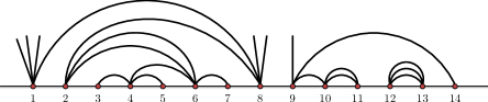
Figure 1.1. Example of a planar $(36,15)$-link pattern of $p=14$ points.

In Section 5, we also prove a further property of the functions $\mathscr{F}_{\omega}$, concerning limits when taking several variables together simultaneously. In terms of the link pattern $\omega$, this means removing several links simultaneously. Such asymptotics pertains to general boundary behavior of the solutions.

Proposition (Proposition 5.6).

For any $1\leq j<k\leq p$ and $\xi\in(x_{j-1},x_{k+1})$, we have

$$\lim_{x_{j},x_{j+1},\ldots,x_{k}\to\xi}\frac{\mathscr{F}_{\omega}(x_{1},\ldots,x_{p})}{\mathscr{F}_{\tau}(x_{j},\ldots,x_{k})}=\; \mathscr{F}_{\omega/\tau}(x_{1},\ldots,x_{j-1},\xi,x_{k+1},\ldots,x_{p}),$$

where $\tau$ denotes the sub-link pattern of $\omega$ between the indices $j,k$ and $\omega/\tau$ denotes the link pattern obtained from $\omega$ by removing $\tau$, as detailed in Section 5.3.

1.1.2. Cyclic permutation symmetry

Solutions of the Benoit & Saint-Aubin PDEs enjoying Möbius covariance play a special role in conformal field theory. In particular, physical correlation functions should transform covariantly under all Möbius maps, by conformal invariance of the theory. In applications to the theory of $\mathrm{SLE}$s, observables such as the multiple $\mathrm{SLE}$ (pure) partition functions also have this property. More generally, in Theorem 5.3 we show also that the solutions $\mathscr{F}_{\omega}$ corresponding to link patterns $\omega$ with zero defects are Möbius covariant. These functions also behave nicely in the limits $x_{1}\to-\infty$ and $x_{p}\to+\infty$, in the following sense.

Proposition (Proposition 5.8).

For any link pattern $\omega$ with no defects $(s=0)$, we have

$$\lim_{y\to+\infty}\Big{(}y^{2h}\times\mathscr{F}_{\omega}(x_{1},\ldots,x_{p-1},y)\Big{)}=\lim_{y\to-\infty}\Big{(}|y|^{2h}\times\mathscr{F}_{\mathcal{S}(\omega)}(y,x_{2},\ldots,x_{p})\Big{)},$$

where $h=h_{1,d_{p}}$ is a Kac weight associated to the point $x_{p}$, and $\mathcal{S}(\omega)$ is a planar link pattern obtained from $\omega$ by a cyclic permutation, as defined in Equation (4.4) in Section 4.

1.1.3. Application to multiple $\mathrm{SLE}$ pure partition functions

Figure 1.2. Example of a planar pair partition of $2N=14$ points.

As a special case of the cyclic permutation symmetry, it follows that the multiple $\mathrm{SLE}$ pure partition functions $\mathcal{Z}_{\alpha}(x_{1},\ldots,x_{2N})$ satisfy a cascade property when $x_{1}\to-\infty$ and $x_{2N}\to+\infty$. In terms of the probability measures of the random curves, we have a natural cascade property concerning the removal of one curve, see [KL07, KP16, PW19].

Corollary (Corollary 6.2).

For any planar pair partition $\alpha$, we have

$$\lim_{\begin{subarray}{c}x_{1}\to-\infty,\\ x_{2N}\to+\infty\end{subarray}}|x_{2N}-x_{1}|^{2h_{1,2}}\times\mathcal{Z}_{\alpha}(x_{1},\ldots,x_{2N})=\; \begin{cases}0\quad&\text{if }\underset{\;1\;\;2N}{\vbox{\hbox{\includegraphics[scale={0.5}]{link-0.pdf}}}}\notin\alpha\\ \mathcal{Z}_{\hat{\alpha}}(x_{2},\ldots,x_{2N-1})&\text{if }\underset{\;1\;\;2N}{\vbox{\hbox{\includegraphics[scale={0.5}]{link-0.pdf}}}}\in\alpha,\end{cases}$$

where $\hat{\alpha}=\alpha/\raisebox{2.15277pt}{ \scalebox{0.75}{$\underset{\;\boldsymbol{1}\;\;\boldsymbol{2N}}{\vbox{\hbox{\includegraphics[scale={0.5}]{link-0.pdf}}}}$}}$, and $h_{1,2}=\frac{6-\kappa}{2\kappa}$, and $\kappa\in(0,8)\setminus\mathbb{Q}$ is the parameter of the $\mathrm{SLE}_{\kappa}$.

1.2. Organization

Our most important results are given in Section 5 (Theorem 5.3 & Proposition 5.6): construction of the solutions $\mathscr{F}_{\omega}$ to the Benoit & Saint-Aubin PDEs, Section 6 (Corollary 6.1): application to the multiple $\mathrm{SLE}$ pure partition functions, and Section 3 (Theorem 3.1): construction of certain basis vectors $\mathfrak{v}_{\omega}$ in tensor product representations of the quantum group $\mathcal{U}_{q}(\mathfrak{sl}_{2})$, which serve as building blocks for the solutions $\mathscr{F}_{\omega}$ with the “spin chain – Coulomb gas correspondence” of [KP20].

Sections 2 – 4 concern the representation theory of the quantum group $\mathcal{U}_{q}(\mathfrak{sl}_{2})$ and the construction and properties of the vectors $\mathfrak{v}_{\omega}$. Sections 5 – 6 treat the solutions $\mathscr{F}_{\omega}$ themselves. In Section 5, we also very briefly discuss the quantum group method of the article [KP20]. Appendices A and B contain auxiliary calculations which are needed in the proofs in Section 3. Appendix C constitutes some additional tools needed to prove the general limiting behavior of the basis functions $\mathscr{F}_{\omega}$.

1.3. Acknowledgments

During this work, the author was supported by Vilho, Yrjö and Kalle Väisälä Foundation and affiliated with the University of Helsinki. She wishes to especially thank Steven Flores and Kalle Kytölä for many inspiring discussions and ideas. She has also enjoyed stimulating and helpful discussions with Michel Bauer, Dmitry Chelkak, Julien Dubédat, Bertrand Duplantier, Philippe Di Francesco, Clément Hongler, Konstantin Izyurov, Jesper Jacobsen, Fredrik Johansson-Viklund, Rinat Kedem, Antti Kemppainen, Jonatan Lenells, Jason Miller, Wei Qian, Hubert Saleur, and Hao Wu. She thanks Roland Friedrich for pointing out important references.

2. Preliminaries: The quantum group $\mathcal{U}_{q}(\mathfrak{sl}_{2})$ and some combinatorics

In this section, we discuss preliminaries concerning the quantum group $\mathcal{U}_{q}(\mathfrak{sl}_{2})$ and its representations, as well as the set of planar link patterns $\omega$ and some combinatorial results. We also introduce notations which will be used and referred to throughout this article.

Fix a parameter $q\in\mathbb{C}\setminus\left\{0\right\}$, and assume that $q^{m}\neq 1$, for all $m\in\mathbb{Z}\setminus\left\{0\right\}$, i.e., that $q$ is not a root of unity. Let $m\in\mathbb{Z}$, and $n,k\in\mathbb{N}$, with $0\leq k\leq n$. We define the $q$-integers as

$$\left[m\right]=\; \frac{q^{m}-q^{-m}}{q-q^{-1}}=q^{m-1}+q^{m-3}+\cdots+q^{3-m}+q^{1-m}$$

and the $q$-factorials and $q$-binomial coefficients as

$$\left[n\right]!=\; \prod_{m=1}^{n}\left[m\right]\qquad\qquad\text{and}\qquad\qquad\left[\begin{array}[]{c}n\\ k\end{array}\right]=\frac{\left[n\right]!}{\left[k\right]!\left[n-k\right]!}.$$

2.1. The quantum group

We define the quantum group $\mathcal{U}_{q}(\mathfrak{sl}_{2})$ as the associative unital algebra over the field $\mathbb{C}$ of complex numbers, with generators $K,K^{-1},E,F$ and relations

$$KK^{-1}= \;1=K^{-1}K,\qquad KE=q^{2}EK,\qquad KF=q^{-2}FK,$$

$$EF-FE= \;\frac{1}{q-q^{-1}}\left(K-K^{-1}\right).$$

The algebra homomorphism

$$\Delta\;\colon\; \mathcal{U}_{q}(\mathfrak{sl}_{2})\rightarrow\mathcal{U}_{q}(\mathfrak{sl}_{2})\otimes\mathcal{U}_{q}(\mathfrak{sl}_{2}),$$

defined by its values on the generators,

(2.1) $$\Delta(E)=E\otimes K+1\otimes E,\qquad\Delta(K)=K\otimes K,\qquad\Delta(F)=F\otimes 1+K^{-1}\otimes F,$$

gives a coproduct on $\mathcal{U}_{q}(\mathfrak{sl}_{2})$, and it determines the unique Hopf algebra structure on the quantum group. Furthermore, using the the coproduct $\Delta$, tensor products of representations of $\mathcal{U}_{q}(\mathfrak{sl}_{2})$ can be equipped with a representation structure as follows. If $M^{\prime}$ and $M^{\prime\prime}$ are two representations, and we have

$$\Delta(X)=\; \sum_{i}X_{i}^{\prime}\otimes X_{i}^{\prime\prime}\,\in\,\mathcal{U}_{q}(\mathfrak{sl}_{2})\otimes\mathcal{U}_{q}(\mathfrak{sl}_{2}),$$

we define the action of $X\in\mathcal{U}_{q}(\mathfrak{sl}_{2})$ on the tensor product $M^{\prime}\otimes M^{\prime\prime}$ by linear extension of the formula

$$X.(v^{\prime}\otimes v^{\prime\prime})=\; \sum_{i}(X_{i}^{\prime}.v^{\prime})\otimes(X_{i}^{\prime\prime}.v^{\prime\prime})\,\in\,M^{\prime}\otimes M^{\prime\prime},$$

for any $v^{\prime}\in M^{\prime}$, $v^{\prime\prime}\in M^{\prime\prime}$. We similarly define tensor product representations with $n$ tensor components using the $(n-1)$-fold coproduct

$$\Delta^{(n)}\colon\mathcal{U}_{q}(\mathfrak{sl}_{2})\rightarrow\Big{(}\mathcal{U}_{q}(\mathfrak{sl}_{2})\Big{)}^{\otimes n},\qquad\Delta^{(n)}=\; (\Delta\otimes\mathrm{id}^{\otimes(n-2)})\circ(\Delta\otimes\mathrm{id}^{\otimes(n-3)})\circ\cdots\circ(\Delta\otimes\mathrm{id})\circ\Delta,$$

and by the coassociativity property $(\mathrm{id}\otimes\Delta)\circ\Delta=(\Delta\otimes\mathrm{id})\circ\Delta$ of the coproduct, there is no need to specify the order in which the tensor products are formed. The multiple coproducts of the generators have the following formulas (see e.g. [KP20, Lemma 2.2]):

(2.2) $$\begin{split}\Delta^{(n)}(K)=\;&K^{\otimes n},\\ \Delta^{(n)}(E)=\;&\sum_{i=1}^{n}1^{\otimes(i-1)}\otimes E\otimes K^{\otimes(n-i)},\\ \Delta^{(n)}(F)=\;&\sum_{i=1}^{n}(K^{-1})^{\otimes(i-1)}\otimes F\otimes 1^{\otimes(n-i)}.\end{split}$$

2.2. Representations of the quantum group

The quantum group $\mathcal{U}_{q}(\mathfrak{sl}_{2})$ has irreducible representations of any dimension $d\in\mathbb{Z}_{>0}$. Given $d$, we always denote $s=d-1$. A $d$-dimensional representation $\mathsf{M}_{d}$ of highest weight $q^{s}$ is obtained by suitably $q$-deforming the irreducible representation of dimension $d$ and highest weight $s$ of the semisimple Lie algebra $\mathfrak{sl}_{2}(\mathbb{C})$: $\mathsf{M}_{d}$ has a basis $e_{0}^{(d)},e_{1}^{(d)},\ldots,e_{s}^{(d)}$ with action

$$K.e_{l}^{(d)}=\; q^{s-2l}\,e_{l}^{(d)},$$

$$F.e_{l}^{(d)}=\; \begin{cases}e_{l+1}^{(d)}&\text{if }l\neq s\\ 0&\text{if }l=s,\end{cases}$$

$$E.e_{l}^{(d)}=\; \begin{cases}\left[l\right]\left[s-l+1\right]\,e_{l-1}^{(d)}&\text{if }l\neq 0\\ 0&\text{if }l=0\end{cases}$$

of the generators $E,F,K$. For simplicity, we usually drop the superscript notation from the basis vectors, writing $e_{l}^{(d)}=e_{l}$. It is well-known that $\mathsf{M}_{d}$ are irreducible, see, e.g., [KP20, Lemma 2.3].

When $q$ is generic (not a root of unity), the representation theory of $\mathcal{U}_{q}(\mathfrak{sl}_{2})$ is semisimple, and in particular, tensor products of representations decompose into direct sums of irreducible subrepresentations. We will make use of the following quantum Clebsch-Gordan decomposition.

Lemma 2.1 (see, e.g., [KP20, Lemma 2.4]).

Let $d_{1},d_{2}\in\mathbb{Z}_{>0}$ and $m\in\{0,1,\ldots,\min(s_{1},s_{2})\}$, where we denote $d=d_{1}+d_{2}-1-2m$ and $s_{1}=d_{1}-1$, $s_{2}=d_{2}-1$. In the representation $\mathsf{M}_{d_{2}}\otimes\mathsf{M}_{d_{1}}$, the vector

(2.3) $$\tau_{0}^{(d;d_{1},d_{2})}=\; \sum_{l_{1},l_{2}=0}^{\min(s_{1},s_{2})}\delta_{l_{1}+l_{2},m}\times(-1)^{l_{1}}\frac{\left[s_{1}-l_{1}\right]!\,\left[s_{2}-l_{2}\right]!}{\left[l_{1}\right]!\left[s_{1}\right]!\left[l_{2}\right]!\left[s_{2}\right]!}\,\frac{q^{l_{1}(s_{1}-l_{1}+1)}}{(q-q^{-1})^{m}}\times(e_{l_{2}}\otimes e_{l_{1}}),$$

is a highest weight vector of a subrepresentation isomorphic to $\mathsf{M}_{d}$, that is, we have

$$E.\tau_{0}^{(d;d_{1},d_{2})}=0\qquad\text{and}\qquad K.\tau_{0}^{(d;d_{1},d_{2})}=q^{s}\,\tau_{0}^{(d;d_{1},d_{2})}.$$

The space $\mathsf{M}_{d_{2}}\otimes\mathsf{M}_{d_{1}}$ has the following decomposition according to the $d$-dimensional subrepresentations:

(2.4) $$\mathsf{M}_{d_{2}}\otimes\mathsf{M}_{d_{1}}\cong\; \mathsf{M}_{d_{1}+d_{2}-1}\oplus\mathsf{M}_{d_{1}+d_{2}-3}\oplus\cdots\oplus\mathsf{M}_{|d_{1}-d_{2}|+3}\oplus\mathsf{M}_{|d_{1}-d_{2}|+1}.$$

For each $d$, the subrepresentation $\mathsf{M}_{d}\subset\mathsf{M}_{d_{2}}\otimes\mathsf{M}_{d_{1}}$ is generated by the highest weight vector $\tau_{0}^{(d;d_{1},d_{2})}$, and we denote by $\tau_{l}^{(d;d_{1},d_{2})}=F^{l}.\tau_{0}^{(d;d_{1},d_{2})}$ the corresponding basis, with $l\in\{0,1,\ldots,s\}$.

2.3. Tensor products of representations

In this article, we consider tensor products

(2.5) $$\bigotimes_{i=1}^{p}\mathsf{M}_{d_{i}}=\; \mathsf{M}_{d_{p}}\otimes\mathsf{M}_{d_{p-1}}\otimes\cdots\otimes\mathsf{M}_{d_{2}}\otimes\mathsf{M}_{d_{1}}$$

of irreducible representations of the quantum group $\mathcal{U}_{q}(\mathfrak{sl}_{2})$, and we use the convention of [KP16, KP20] for the order of tensorands, as explicitly written on the right hand side. We occasionally abbreviate the tensor product as above, in which case the reverse order of tensorands is implicit. By the coassociativity property of the coproduct, repeated application of the decomposition (2.4) gives the direct sum formula

(2.6) $$\mathsf{M}_{d_{p}}\otimes\cdots\otimes\mathsf{M}_{d_{1}}\cong\bigoplus_{d}m_{d}\,\mathsf{M}_{d},$$

where the subrepresentations isomorphic to $\mathsf{M}_{d}$ now have multiplicities $m_{d}=m_{d}(d_{1},\ldots,d_{p})$.

Throughout this article, it is convenient to denote by

(2.7) $$s=d-1,\qquad s_{i}=d_{i}-1,\quad\text{ for all }i\in\{1,2,\ldots,p\},\qquad\text{ and }\qquad\varsigma=(s_{1},s_{2},\ldots,s_{p})\in\mathbb{Z}_{\geq 0}^{p}.$$

For $d=s+1$, the $m_{d}$ copies of $\mathsf{M}_{d}$ are generated by highest weight vectors of weight $q^{s}$. We denote by

(2.8) $$\mathsf{H}_{\varsigma}^{(s)}=\; \Big{\{}v\in\bigotimes_{i=1}^{p}\mathsf{M}_{d_{i}}\;\big{|}\;E.v=0,\;K.v=q^{s}\,v\Big{\}}$$

the $m_{d}$-dimensional subspace consisting of such vectors. The dimensions $m_{d}$ satisfy a recursion equation, given in Lemma 2.2, and they can be calculated by counting certain type of planar link patterns.

2.4. Projections to subrepresentations

Fix $j\in\{1,2,\ldots,p-1\}$. We decompose the $j$:th and $(j+1)$:st tensor components in (2.5) according to the quantum Clebsch-Gordan formula (2.4), and denote the embedding of the $d$-dimensional component in the $j$:th and $(j+1)$:st tensor positions by

(2.9) $$\begin{split}&\iota_{j}^{(d)}=\iota_{j,j+1}^{(d;d_{j},d_{j+1})}\;\colon\;\Big{(}\bigotimes_{i=j+2}^{p}\mathsf{M}_{d_{i}}\Big{)}\otimes\mathsf{M}_{d}\otimes\Big{(}\bigotimes_{i=1}^{j-1}\mathsf{M}_{d_{i}}\Big{)}\;\to\;\bigotimes_{i=1}^{p}\mathsf{M}_{d_{i}}\\ &\iota_{j}^{(d)}\left(e_{l_{p}}\otimes\cdots\otimes e_{l_{j+2}}\otimes e_{l}\otimes e_{l_{j-1}}\otimes\cdots\otimes e_{l_{1}}\right)=e_{l_{p}}\otimes\cdots\otimes e_{l_{j+2}}\otimes\tau_{l}^{(d;d_{j},d_{j+1})}\otimes e_{l_{j-1}}\otimes\cdots\otimes e_{l_{1}}.\end{split}$$

Via the embedding (2.9), we identify the shorter tensor product as a subrepresentation of (2.5),

(2.10) $$\Big{(}\bigotimes_{i=j+2}^{p}\mathsf{M}_{d_{i}}\Big{)}\otimes\mathsf{M}_{d}\otimes\Big{(}\bigotimes_{i=1}^{j-1}\mathsf{M}_{d_{i}}\Big{)}\,\subset\,\; \bigotimes_{i=1}^{p}\mathsf{M}_{d_{i}},$$

and denote by

(2.11) $$\pi_{j}^{(d)}=\pi_{j,j+1}^{(d;d_{j},d_{j+1})}\;\colon\; \bigotimes_{i=1}^{p}\mathsf{M}_{d_{i}}\to\bigotimes_{i=1}^{p}\mathsf{M}_{d_{i}}$$

the projection to this subrepresentation — by definition, a vector $v\in\bigotimes_{i=1}^{p}\mathsf{M}_{d_{i}}$ lies in the subrepresentation (2.10) if and only if we have $\pi_{j}^{(d)}(v)=v$. We further let

$$\hat{\pi}_{j}^{(d)}=\hat{\pi}_{j,j+1}^{(d;d_{j},d_{j+1})}\;\colon\; \bigotimes_{i=1}^{p}\mathsf{M}_{d_{i}}\to\Big{(}\bigotimes_{i=j+2}^{p}\mathsf{M}_{d_{i}}\Big{)}\otimes\mathsf{M}_{d}\otimes\Big{(}\bigotimes_{i=1}^{j-1}\mathsf{M}_{d_{i}}\Big{)}$$

denote the projection (2.11) combined with the identification (2.10) — the identity $\pi_{j}^{(d)}=\iota_{j}^{(d)}\circ\hat{\pi}_{j}^{(d)}$ then holds.

More generally, for $m\in\{0,1,\ldots,\min(d_{j},d_{j+1})-1\}$ and $d=d_{j}+d_{j+1}-1-2m$, we define the map

(2.12) $$\begin{split}&\widetilde{\pi}_{j}^{(d)}=\widetilde{\pi}_{j,j+1}^{(d;d_{j},d_{j+1})}\;\colon\;\bigotimes_{i=1}^{p}\mathsf{M}_{d_{i}}\;\to\;\Big{(}\bigotimes_{i=j+2}^{p}\mathsf{M}_{d_{i}}\Big{)}\otimes\mathsf{M}_{d_{j+1}-m}\otimes\mathsf{M}_{d_{j}-m}\otimes\Big{(}\bigotimes_{i=1}^{j-1}\mathsf{M}_{d_{i}}\Big{)}\\ &\widetilde{\pi}_{j,j+1}^{(d;d_{j},d_{j+1})}:=\iota_{j,j+1}^{(d;d_{j}-m,d_{j+1}-m)}\circ\hat{\pi}_{j,j+1}^{(d;d_{j},d_{j+1})},\end{split}$$

whose image is a subrepresentation of type (2.10), having the subrepresentation of $\mathsf{M}_{d_{j+1}-m}\otimes\mathsf{M}_{d_{j}-m}$ isomorphic to $\mathsf{M}_{d}$ in the $j$:th and $(j+1)$:st tensor positions.

The trivial representation $\mathsf{M}_{1}$ is the neutral element for tensor products of representations. We always identify it with the complex numbers $\mathbb{C}$, via $\tau_{0}^{(1;d_{j},d_{j+1})}\mapsto 1$, and omit it from the tensor products. The image of the projection $\hat{\pi}_{j}^{(1)}$ thus lies in the shorter tensor product $\Big{(}\bigotimes_{i=j+2}^{p}\mathsf{M}_{d_{i}}\Big{)}\otimes\Big{(}\bigotimes_{i=1}^{j-1}\mathsf{M}_{d_{i}}\Big{)}$, and for $m=\min(d_{j},d_{j+1})-1$, the embedding $\iota_{j,j+1}^{(d;d_{j}-m,d_{j+1}-m)}$ reduces to the identity map.

2.5. Planar link patterns

Tensor product representations of type (2.6) have bases indexed by planar link patterns, where each highest weight vector corresponds to a link pattern, and the other basis elements are obtained by action of the generator $F$. For example, a relatively well-known fact is that the tensor power $\mathsf{M}_{2}^{\otimes n}$ of two-dimensional irreducibles has such a basis; see e.g. [Jim86, Lus92, Mar92, FK97, PSA14, RSA14]. In this case, for each $s\in\mathbb{Z}_{\geq 0}$ the space (2.8) of highest weight vectors in $\mathsf{M}_{2}^{\otimes n}$ admits a natural diagrammatic action of the Temperley-Lieb algebra, known as the link-state representation. For $s=0$, $n$ is even, and the link states are indexed by planar pair partitions of $n/2$ points, see Figure 1.2. For $s>0$, there are also additional lines called defects, see Figure 2.1.

In the present article, we consider general link patterns, which are useful in calculations concerning general tensor product representations of type (2.6). The planar pair partitions then arise as a special case. A word of warning is in order here: the bases of the tensor product representations of type (2.6) which we construct in Section 3 do not carry the “usual” link-state action of diagram algebras such as the Temperley-Lieb algebra, even in the special case of $\mathsf{M}_{2}^{\otimes n}$. In fact, the basis we construct in the present article is the dual basis of the “canonical basis” [Lus92, FK97]. However, we will not pursue this direction here — our interests lie in constructing solutions to the Benoit & Saint-Aubin PDE systems with given asymptotics properties, using the quantum group rather as a tool.

Denote the upper half-plane by $\mathbb{H}=\left\{z\in\mathbb{C}\;|\;\Im\mathfrak{m}(z)>0\right\}$. Fix a multiindex $\varsigma=(s_{1},\ldots,s_{p})\in\mathbb{Z}_{>0}^{p}$, and let $\ell\in\mathbb{Z}_{\geq 0}$ be an integer such that $2\ell\leq n$, where we denote

(2.13) $$n=|\varsigma|:=\sum_{i=1}^{p}s_{i}\qquad\text{ and }\qquad s=n-2\ell\,\in\,\mathbb{Z}_{\geq 0}.$$

We define planar ($n,\ell$)-link patterns of $p$ points with index valences $\varsigma=(s_{1},\ldots,s_{p})$ as collections

$$\omega=\Big{\{}\underset{\;a_{1}\;\;b_{1}}{\vbox{\hbox{\includegraphics[scale={0.5}]{link-0.pdf}}}},\ldots,\underset{\;a_{\ell}\;\;b_{\ell}}{\vbox{\hbox{\includegraphics[scale={0.5}]{link-0.pdf}}}}\Big{\}}\bigcup\Big{\{}\underset{c_{1}}{\vbox{\hbox{\includegraphics[scale={0.5}]{defect-0.pdf}}}},\ldots,\underset{c_{s}}{\vbox{\hbox{\includegraphics[scale={0.5}]{defect-0.pdf}}}}\Big{\}}$$

of

• $\ell$ links of type $\underset{\;\boldsymbol{a\;}\;\;\boldsymbol{\;b\,}}{\vbox{\hbox{\includegraphics[scale={0.5}]{link-0.pdf}}}}$ in $\mathbb{H}$, which connect a pair $a<b$ of indices $a,b\in\{1,2,\ldots,p\}$, and

• $s=n-2\ell$ defects of type $\underset{\boldsymbol{c}}{\vbox{\hbox{\includegraphics[scale={0.5}]{defect-0.pdf}}}}$ in $\mathbb{H}$, attached to an index $c\in\{1,2,\ldots,p\}$,

such that

• for any $i\in\{1,2,\ldots,p\}$, the index $i$ is an endpoint of exactly $s_{i}$ links and defects,

• all the defects lie in the unbounded component of the complement of the set of links in $\mathbb{H}$, and

• none of the links and defects intersect in $\mathbb{H}$, but only at their common endpoints in $\mathbb{N}\subset\mathbb{R}$.

Figure 1.1 shows an example of a planar link pattern. We denote by $\mathrm{LP}^{(s)}_{\varsigma}$ the set of planar ($n,\ell$)-link patterns of $p$ points with index valences $\varsigma=(s_{1},\ldots,s_{p})$, having $s=n-2\ell$ defects. We usually omit the word “planar” when we speak of link patterns.

Because the planar pair partitions play a special role in this article, we denote the set of them by

$$\mathrm{PP}_{N}:=\mathrm{LP}^{(0)}_{(1,1,\ldots,1,1)},\quad\text{ for }N\in\mathbb{Z}_{>0},\qquad\text{ and }\qquad\mathrm{PP}_{0}:=\mathrm{LP}^{(0)}_{()}=\left\{\emptyset\right\},\quad\text{ for }N=0.$$

We also set $\mathrm{PP}=\bigsqcup_{N\geq 0}\mathrm{PP}_{N}$.

More generally, if $\varsigma=(1,1,\ldots,1,1)\in\mathbb{Z}^{n}$ for $n=2N+s$, we denote by $\mathrm{PP}_{N}^{(s)}:=\mathrm{LP}^{(s)}_{(1,1,\ldots,1,1)}$ the set of planar $(n,N)$-link patterns each of which consists of a planar pair partition of $2N$ points and $s$ defects — see Figure 2.1 for an example. The set of planar pair partitions then corresponds to $\mathrm{PP}_{N}=\mathrm{PP}_{N}^{(0)}$.

Figure 2.1. Example of a planar pair partition with defects.

Next, we consider the tensor product representation (2.5), with dimensions $d_{1},\ldots,d_{p}\geq 2$ related to the multiindex $\varsigma$ as in (2.7). The dimension of the subspace $\mathsf{H}_{\varsigma}^{(s)}$ of highest weight vectors of weight $q^{s}$ can be calculated by counting the planar link patterns in $\mathrm{LP}_{\varsigma}^{(s)}$.

Lemma 2.2.

For each $s\in\mathbb{Z}_{\geq 0}$, we have $\mathrm{dim}\mathsf{H}_{\varsigma}^{(s)}=\#\mathrm{LP}_{\varsigma}^{(s)}$.

Proof.

Fix $s\in\mathbb{Z}_{\geq 0}$. The claim follows from the fact that both sides of the asserted equation,

$$D_{\varsigma}^{(s)}:=\mathrm{dim}\mathsf{H}_{\varsigma}^{(s)}\qquad\text{and}\qquad N_{\varsigma}^{(s)}:=\#\mathrm{LP}_{\varsigma}^{(s)},$$

satisfy the same recursion with the same initial condition. If $p=1$, then obviously $D_{(s_{1})}^{(s)}=\delta_{s,s_{1}}=N_{(s_{1})}^{(s)}$. For general $\varsigma=(s_{1},\ldots,s_{p})\in\mathbb{Z}_{>0}^{p}$, consider first the dimension $D_{\varsigma}^{(s)}$ of $\mathsf{H}_{\varsigma}^{(s)}$. Using the notations (2.7), the direct sum decomposition (2.6) of $p$ irreducibles, with $m_{d}=D_{\varsigma}^{(s)}$, can be written recursively as

(2.14) $$\bigoplus_{d}D_{\varsigma}^{(s)}\;\mathsf{M}_{d}=\mathsf{M}_{d_{p}}\otimes(\mathsf{M}_{d_{p-1}}\otimes\cdots\otimes\mathsf{M}_{d_{1}})=\mathsf{M}_{d_{p}}\otimes\Big{(}\bigoplus_{\hat{d}}D_{\hat{\varsigma}}^{(\hat{s})}\;\mathsf{M}_{\hat{d}}\Big{)}=\bigoplus_{\hat{d}}D_{\hat{\varsigma}}^{(\hat{s})}\left(\mathsf{M}_{d_{p}}\otimes\mathsf{M}_{\hat{d}}\right),$$

where $\hat{s}=\hat{d}-1$ and $\hat{\varsigma}=(s_{1},\ldots,s_{p-1})$, by the coassociativity property of the coproduct of $\mathcal{U}_{q}(\mathfrak{sl}_{2})$. Using the explicit decomposition (2.4) of the tensor product of two irreducibles, we obtain the recursion

$$D_{\varsigma}^{(s)}=\sum_{k\geq 0}D_{\hat{\varsigma}}^{(s-s_{p}+2k)},$$

where the numbers $D_{\hat{\varsigma}}^{(s-s_{p}+2k)}$ are zero when $k$ is large enough (and for small $k$ in some cases).

Consider then the number $N_{\varsigma}^{(s)}$ of link patterns with $s$ defects. We classify the link patterns $\omega\in\mathrm{LP}_{\varsigma}^{(s)}$ according to the number $k$ of links having the endpoint $p$ (so there are $s_{p}-k$ defects having the endpoint $p$). Imagine cutting the point $p$ off from the link pattern $\omega$. Then, the remaining points $1,2,\ldots,p-1$ will have $\hat{s}=s-(s_{p}-k)+k=s-s_{p}+2k$ defects in total — see Figure 2.2 — namely, the $s-(s_{p}-k)$ defects inherited from $\omega$ and in addition $k$ defects attached to the $k$ links which had the endpoint $p$. This gives the same recursion as above:

$$N_{\varsigma}^{(s)}=\sum_{k\geq 0}N_{\hat{\varsigma}}^{(s-s_{p}+2k)}.$$

It follows that $D_{\varsigma}^{(s)}=N_{\varsigma}^{(s)}$, as claimed. ∎

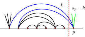
Figure 2.2. Illustration of the recursion used in the proof of Lemma 2.2. When cutting the point $p$ off from the link pattern, the blue links become defects.

2.6. Combinatorial maps

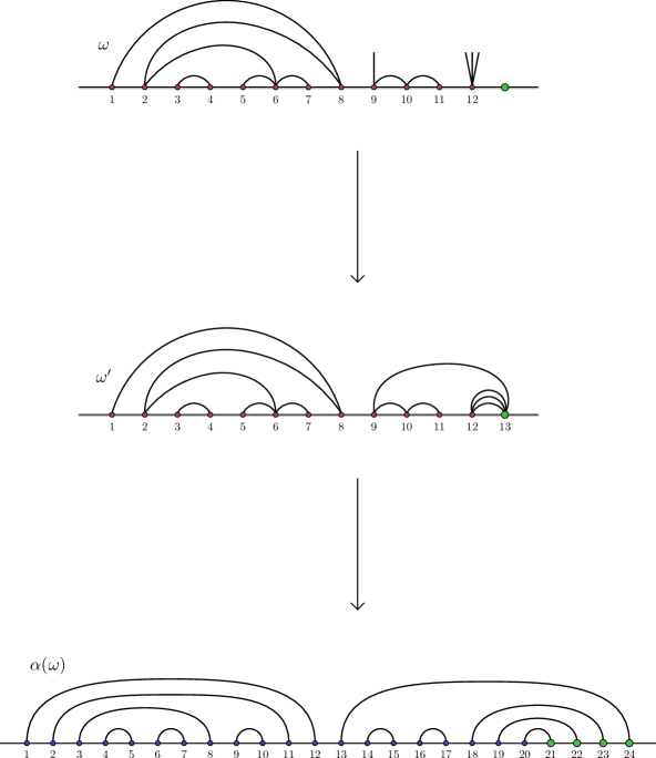
Figure 2.3. Illustration of the map $\varphi\colon\omega\mapsto\alpha(\omega)$, defined as the composition $\varphi=\mathcal{I}\circ\mathcal{R}_{+}^{-1}$. The middle figure illustrates the image of $\omega$ under the first map, that is, $\omega^{\prime}=\mathcal{R}_{+}^{-1}(\omega)$, where the defects of $\omega$ are attached to an additional index $p+1$ on the right of all the other indices. The lowest figure depicts the planar pair partition $\alpha(\omega)$, which is obtained from $\omega^{\prime}$ by “opening up” all the points, that is, splitting each index $i$ to $s_{i}$ new indices and taking the lines of $i$ along with the points.

We next define a natural map, which associates to each planar link pattern $\omega\in\mathrm{LP}^{(s)}_{\varsigma}$ a planar pair partition $\alpha=\alpha(\omega)\in\mathrm{PP}_{N}$, such that

(2.15) $$N=\frac{1}{2}\left(\sum_{i=1}^{p}s_{i}+s\right)=\frac{n+s}{2}=\ell+s.$$

This map, denoted by

(2.16) $$\varphi\;\colon\;\mathrm{LP}^{(s)}_{\varsigma}\rightarrow\mathrm{PP}_{N},\qquad\omega\mapsto\alpha(\omega),$$

is defined as a composition $\varphi=\mathcal{I}\circ\mathcal{R}_{+}^{-1}$ of the two combinatorial maps

$$\mathcal{R}_{+}^{-1}=(\mathcal{R}_{+}^{(s)})^{-1}\; \colon\;\mathrm{LP}^{(s)}_{\varsigma}\rightarrow\mathrm{LP}^{(0)}_{(\varsigma,s)},\qquad\text{ and }\qquad\mathcal{I}=\mathcal{I}_{(\varsigma,s)}\;\colon\;\mathrm{LP}^{(0)}_{(\varsigma,s)}\rightarrow\mathrm{PP}_{N},$$

which we define shortly — see also Figure 2.3 for an illustration.

We first define $\mathcal{R}_{+}^{-1}$ and its inverse map $\mathcal{R}_{+}\colon\mathrm{LP}^{(0)}_{(\varsigma,s)}\to\mathrm{LP}^{(s)}_{\varsigma}$. Consider a link pattern

$$\omega=\Big{\{}\underset{\;a_{1}\;\;b_{1}}{\vbox{\hbox{\includegraphics[scale={0.5}]{link-0.pdf}}}},\ldots,\underset{\;a_{\ell}\;\;b_{\ell}}{\vbox{\hbox{\includegraphics[scale={0.5}]{link-0.pdf}}}}\Big{\}}\bigcup\Big{\{}\underset{c_{1}}{\vbox{\hbox{\includegraphics[scale={0.5}]{defect-0.pdf}}}},\ldots,\underset{c_{s}}{\vbox{\hbox{\includegraphics[scale={0.5}]{defect-0.pdf}}}}\Big{\}}\,\in\,\mathrm{LP}^{(s)}_{\varsigma}.$$

Introduce an additional index $p+1$, of valence $s_{p+1}=s$, and connect the defects of $\omega$ to it, to form

$$\omega^{\prime}=\Big{\{}\underset{\;a_{1}\;\;b_{1}}{\vbox{\hbox{\includegraphics[scale={0.5}]{link-0.pdf}}}},\ldots,\underset{\;a_{\ell}\;\;b_{\ell}}{\vbox{\hbox{\includegraphics[scale={0.5}]{link-0.pdf}}}},\underset{\;c_{1}\;\;p+1}{\vbox{\hbox{\includegraphics[scale={0.5}]{link-0.pdf}}}},\underset{\;c_{2}\;\;p+1}{\vbox{\hbox{\includegraphics[scale={0.5}]{link-0.pdf}}}},\ldots,\underset{\;c_{s}\;\;p+1}{\vbox{\hbox{\includegraphics[scale={0.5}]{link-0.pdf}}}}\Big{\}}\,\in\,\mathrm{LP}^{(0)}_{(\varsigma,s)},$$

a link pattern of $p+1$ points having index valences $(\varsigma,s):=(s_{1},\ldots,s_{p},s)$ and zero defects. Set

$$\mathcal{R}_{+}^{-1}(\omega):=\omega^{\prime}.$$

This defines the map $\mathcal{R}_{+}^{-1}\colon\mathrm{LP}^{(s)}_{\varsigma}\rightarrow\mathrm{LP}^{(0)}_{(\varsigma,s)}$. It has an obvious inverse map $\mathcal{R}_{+}=\mathcal{R}_{+}^{(s)}\;\colon\;\mathrm{LP}^{(0)}_{(\varsigma,s)}\rightarrow\mathrm{LP}^{(s)}_{\varsigma}$ obtained by removing the last index $p+1$ of valence $s$ so that the links attached to it become defects. We similarly define $\mathcal{R}_{-}=\mathcal{R}_{-}^{(s)}\colon\mathrm{LP}^{(0)}_{(s,\varsigma)}\rightarrow\mathrm{LP}^{(s)}_{\varsigma}$ and its inverse map $\mathcal{R}_{-}^{-1}=(\mathcal{R}_{-}^{(s)})^{-1}\colon\mathrm{LP}^{(s)}_{\varsigma}\rightarrow\mathrm{LP}^{(0)}_{(s,\varsigma)}$ by removing (resp. adding) the index $1$ and relabeling the other indices from left to right by $1,2,\ldots,p$ (resp. $2,3,\ldots,p+1$).

To define the map $\mathcal{I}=\mathcal{I}_{(\varsigma,s)}$, split each index $i\in\{1,2,\ldots,p+1\}$ of $\omega^{\prime}$ to $s_{i}$ distinct indices, with $s_{p+1}=s$, and attach the $s_{i}$ links ending at $i$ in $\omega^{\prime}$ to these new $s_{i}$ indices, so that each of them has valence one (see Figure 2.3). This results in a diagram with $2N=\sum_{i=1}^{p}s_{i}+s$ indices, each of which has valence one. Label these indices from left to right by $1,2,\ldots,2N$, to obtain the planar pair partition

$$\mathcal{I}(\omega^{\prime})=\alpha(\omega)\,\in\,\mathrm{LP}^{(0)}_{(1,1,\ldots,1,1)}=\mathrm{PP}_{N}.$$

This finally defines the map $\mathcal{I}\colon\mathrm{LP}^{(0)}_{(\varsigma,s)}\rightarrow\mathrm{PP}_{N}$ and thus the map $\varphi=\mathcal{I}\circ\mathcal{R}_{+}^{-1}$.

2.7. Properties of the link patterns

To finish, we introduce some notation concerning the recursive structure of the set of planar link patterns, to be used throughout this article.

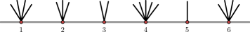
Figure 2.4. Example of a link pattern $\shuffle_{\lambda}$ for a partition $\lambda=(4,3,2,5,1,4)$.

2.7.1. Defects and partitions

Integer partitions $\lambda=(s_{1},\ldots,s_{|\lambda|})$ of $s$ correspond naturally to endpoints of defects in planar link patterns. A partition $\lambda$ of $s$ determines a unique $(s,0)$-link pattern denoted by $\shuffle_{\lambda}\in\mathrm{LP}^{(s)}_{\lambda}$, which consists of $s$ defects with endpoints $i=1,2\ldots,|\lambda|$, having valences $s_{i}=s_{i}$ specified by $\lambda$, as in Figure 2.4. We also include the $(0,0)$-link pattern $\shuffle_{()}=\emptyset$ for $s=0$.

Conversely, let $\varsigma\in\mathbb{Z}_{>0}^{p}$ and consider an $(n,\ell)$-link pattern with $s=n-2\ell$ defects, with notations (2.13),

$$\omega=\Big{\{}\underset{\;a_{1}\;\;b_{1}}{\vbox{\hbox{\includegraphics[scale={0.5}]{link-0.pdf}}}},\ldots,\underset{\;a_{\ell}\;\;b_{\ell}}{\vbox{\hbox{\includegraphics[scale={0.5}]{link-0.pdf}}}}\Big{\}}\bigcup\Big{\{}\underset{c_{1}}{\vbox{\hbox{\includegraphics[scale={0.5}]{defect-0.pdf}}}},\ldots,\underset{c_{s}}{\vbox{\hbox{\includegraphics[scale={0.5}]{defect-0.pdf}}}}\Big{\}}\,\in\,\mathrm{LP}^{(s)}_{\varsigma}.$$

When $s\geq 1$, the set $\big{\{}\raisebox{2.15277pt}{ \scalebox{0.75}{$\underset{\boldsymbol{c_{1}}}{\vbox{\hbox{\includegraphics[scale={0.5}]{defect-0.pdf}}}}$}},\ldots,\raisebox{2.15277pt}{ \scalebox{0.75}{$\underset{\boldsymbol{c_{s}}}{\vbox{\hbox{\includegraphics[scale={0.5}]{defect-0.pdf}}}}$}}\big{\}}$ of defects in $\omega$ defines naturally a partition of $s$ as follows: if $\left\{u_{1},\ldots,u_{t}\right\}\subset\left\{1,\ldots,p\right\}$, for $u_{1}<\ldots<u_{t}$, denote the distinct endpoints of the defects in $\omega$ with multiplicities given by the number $r_{i}(\omega)=\#\left\{k\;|\;c_{k}=u_{i}\right\}\geq 1$ of defects ending at the index $u_{i}$, then we have $s=\sum_{i=1}^{t}r_{i}(\omega)$, and the numbers $r_{i}(\omega)$ thus define a partition of $s$ into $t$ positive integers,

$$\lambda(\omega)=\big{(}r_{1}(\omega),\ldots,r_{t}(\omega)\big{)}.$$

We denote the set of all planar link patterns with a fixed number $s\in\mathbb{Z}_{\geq 0}$ of defects by

$$\mathrm{LP}^{(s)}=\bigsqcup_{p\in\mathbb{N},\;\varsigma\in\mathbb{Z}_{>0}^{p}}\mathrm{LP}^{(s)}_{\varsigma},$$

and, for a fixed partition $\lambda=(s_{1},\ldots,s_{|\lambda|})$ of $s$, we denote by

$$\mathrm{LP}^{(s)}(\lambda)=\left\{\omega\in\mathrm{LP}^{(s)}\;|\;\lambda(\omega)=\lambda\right\}\qquad\text{ and }\qquad\mathrm{LP}^{(0)}()=\mathrm{LP}^{(0)}$$

the set of all planar link patterns whose defects $\big{\{}\raisebox{2.15277pt}{ \scalebox{0.75}{$\underset{\boldsymbol{c_{1}}}{\vbox{\hbox{\includegraphics[scale={0.5}]{defect-0.pdf}}}}$}},\ldots,\raisebox{2.15277pt}{ \scalebox{0.75}{$\underset{\boldsymbol{c_{s}}}{\vbox{\hbox{\includegraphics[scale={0.5}]{defect-0.pdf}}}}$}}\big{\}}$ define the partition $\lambda(\omega)=\lambda$.

2.7.2. Removing links

Also the links in the $(n,\ell)$-link pattern

$$\omega=\Big{\{}\underset{\;a_{1}\;\;b_{1}}{\vbox{\hbox{\includegraphics[scale={0.5}]{link-0.pdf}}}},\ldots,\underset{\;a_{\ell}\;\;b_{\ell}}{\vbox{\hbox{\includegraphics[scale={0.5}]{link-0.pdf}}}}\Big{\}}\bigcup\Big{\{}\underset{c_{1}}{\vbox{\hbox{\includegraphics[scale={0.5}]{defect-0.pdf}}}},\ldots,\underset{c_{s}}{\vbox{\hbox{\includegraphics[scale={0.5}]{defect-0.pdf}}}}\Big{\}}\,\in\,\mathrm{LP}^{(s)}_{\varsigma}$$

appear with multiplicity. For two indices $a<b$, we denote by $\ell_{a,b}=\ell_{a,b}(\omega)$ the multiplicity of the link $\underset{\;\boldsymbol{a\;}\;\;\boldsymbol{b\;}}{\vbox{\hbox{\includegraphics[scale={0.5}]{link-0.pdf}}}}$ in $\omega$, that is, we have $\ell_{a,b}=\#\left\{i\;|\;a_{i}=a,b_{i}=b\right\}$ and $\ell=\sum_{k,l}\ell_{k,l}$. In particular, the links of $\omega$ can be regarded as a multiset of $k\leq\ell=\sum_{a,b}\ell_{a,b}$ elements,

$$\mathfrak{L}(\omega)=\Big{\{}\ell_{a_{1},b_{1}}\times\underset{\;a_{1}\;\;b_{1}}{\vbox{\hbox{\includegraphics[scale={0.5}]{link-0.pdf}}}},\;\ldots,\;\ell_{a_{k},b_{k}}\times\underset{\;a_{k}\;\;b_{k}}{\vbox{\hbox{\includegraphics[scale={0.5}]{link-0.pdf}}}}\Big{\}}.$$

Removing one link from an $(n,\ell)$-link pattern determines an $(n-2,\ell-1)$-link pattern. If the removed link had an endpoint with valence one, then the endpoint must be removed as well, and the remaining indices must be relabeled so as to form the endpoints of the smaller link pattern, as illustrated in Figure 2.5. We denote the removal of a link $\underset{\;\boldsymbol{a\;}\;\;\boldsymbol{\;b\,}}{\vbox{\hbox{\includegraphics[scale={0.5}]{link-0.pdf}}}}$ from a link pattern $\omega$ by $\omega/\raisebox{2.15277pt}{ \scalebox{0.75}{$\underset{\;\boldsymbol{a\;}\;\;\boldsymbol{\;b\,}}{\vbox{\hbox{\includegraphics[scale={0.5}]{link-0.pdf}}}}$}}$.

More generally, if the link $\underset{\;\boldsymbol{a\;}\;\;\boldsymbol{\;b\,}}{\vbox{\hbox{\includegraphics[scale={0.5}]{link-0.pdf}}}}$ appears in $\omega\in\mathrm{LP}^{(s)}_{\varsigma}$ with multiplicity $\ell_{a,b}$, we can remove $m\leq\ell_{a,b}$ links from $\omega$. The removal of $m$ links $\underset{\;\boldsymbol{a\;}\;\;\boldsymbol{\;b\,}}{\vbox{\hbox{\includegraphics[scale={0.5}]{link-0.pdf}}}}$ from $\omega$ is then denoted by $\omega/(m\times\raisebox{2.15277pt}{ \scalebox{0.75}{$\underset{\;\boldsymbol{a\;}\;\;\boldsymbol{\;b\,}}{\vbox{\hbox{\includegraphics[scale={0.5}]{link-0.pdf}}}}$}})$. In this case, if $s_{j}=m$ or $s_{j+1}=m$, we have to also remove the index $j$ or $j+1$, respectively (or both), and relabel the indices of the remaining links and defects, as also illustrated in Figure 2.5.

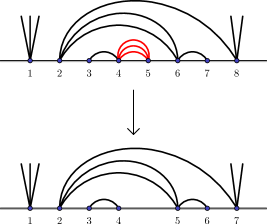
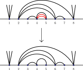
Figure 2.5. Removal of links between the indices $a=4$ and $b=5$. In the left figure, all three links are removed, so the index $5$ has to be removed as well (because it becomes empty, i.e., its valence becomes equal to zero), and the remaining indices are labeled accordingly. On the right, only two links are removed, so the indices remain the same.

3. Basis vectors in quantum group representations

In this section, we construct a basis for each highest weight vector space $\mathsf{H}_{\varsigma}^{(s)}$ (defined in Equation (2.8)) whose vectors are uniquely characterized by certain recursive properties, concerning projections onto subrepresentations. These basis vectors are crucial in our construction of the basis for solutions to the Benoit & Saint-Aubin PDEs in Section 5. The defining properties of the basis vectors correspond to the asymptotic boundary conditions for the basis functions, as explained in Section 5.

In view of Lemma 2.2, it is natural to index the basis vectors $\mathfrak{v}_{\omega}$ by link patterns $\omega$. Specifically, we consider the following system of equations for vectors $\mathfrak{v}_{\omega}\in\bigotimes_{i=1}^{p}\mathsf{M}_{d_{i}}$, with $\omega\in\mathrm{LP}^{(s)}_{\varsigma}$:

(3.1) $$K.\mathfrak{v}_{\omega}=q^{s}\,\mathfrak{v}_{\omega}$$

(3.2) $$E.\mathfrak{v}_{\omega}=0$$

(3.3) $$\widetilde{\pi}_{j}^{(\delta)}(\mathfrak{v}_{\omega})=\begin{cases}\frac{1}{\mathcal{C}({m;s_{j},s_{j+1}})}\times\mathfrak{v}_{\hat{\omega}}&\mbox{if there are at least $m$ links }\underset{\;j\;\;j+1}{\vbox{\hbox{\includegraphics[scale={0.5}]{link-0.pdf}}}}\text{ in }\omega\\ 0&\mbox{otherwise,}\end{cases}$$

$$\text{for all }j\in\{1,2,\ldots,p-1\},\;m\in\{1,2,\ldots,\min(s_{j},s_{j+1})\},\text{ and }\delta=s_{j}+s_{j+1}+1-2m,$$

where $\hat{\omega}=\omega/(m\times\raisebox{2.15277pt}{ \scalebox{0.75}{$\underset{\;\boldsymbol{j}\;\;\boldsymbol{j+1}}{\vbox{\hbox{\includegraphics[scale={0.5}]{link-0.pdf}}}}$}})$, and the constants in (3.3) are non-zero and explicit:

(3.10) $$\mathcal{C}({m;s_{j},s_{j+1}})=\frac{\left[s_{j}-m\right]!\left[s_{j+1}-m\right]!\left[s_{j}+s_{j+1}-m+1\right]!}{\left[2\right]^{m}\left[s_{j}\right]!\left[s_{j+1}\right]!\left[s_{j}+s_{j+1}-2m+1\right]!}=\frac{\left[\begin{array}[]{c}s_{j}+s_{j+1}-m+1\\ m\end{array}\right]}{\left[2\right]^{m}\left[m\right]!\left[\begin{array}[]{c}s_{j}\\ m\end{array}\right]\left[\begin{array}[]{c}s_{j+1}\\ m\end{array}\right]},$$

and where we use, by default, the notations (2.7) for the parameters $s$, $s_{j}$, $s_{j+1}$, and $d=s+1$.

Equations (3.1) – (3.2) state that each $\mathfrak{v}_{\omega}$ belongs to the highest weight vector space $\mathsf{H}_{\varsigma}^{(s)}$. Equations (3.3) concern projections of $\mathfrak{v}_{\omega}$ to subrepresentations, corresponding to removing links from the link pattern $\omega$.

Theorem 3.1.

(a):

For each integer $s\geq 0$, there exists a unique collection $\left(\mathfrak{v}_{\omega}\right)_{\omega\in\mathrm{LP}^{(s)}}$ of vectors such that the system of equations (3.1) – (3.3) holds for all $\omega\in\mathrm{LP}^{(s)}$, we have $\mathfrak{v}_{\emptyset}=1$, and

(3.11) $$\mathfrak{v}_{\shuffle_{\lambda}}=\frac{1}{(q-q^{-1})^{s}}\frac{\left[2\right]^{s}}{\left[s+1\right]!}\times(e_{0}^{(s_{|\lambda|}+1)}\otimes\cdots\otimes e_{0}^{(s_{1}+1)})\,\in\,\mathsf{H}_{\lambda}^{(s)},$$

for any partition $\lambda=(s_{1},\ldots,s_{|\lambda|})$ of $s\geq 1$.

(b):

For fixed $\varsigma\in\mathbb{Z}_{>0}^{p}$, the collection $\left(\mathfrak{v}_{\omega}\right)_{\omega\in\mathrm{LP}^{(s)}_{\varsigma}}$ is a basis of the vector space $\mathsf{H}_{\varsigma}^{(s)}$. In particular,

$$\big{\{}F^{l}.\mathfrak{v}_{\omega}\;|\;\omega\in\mathrm{LP}^{(s)}_{\varsigma},\;l\in\{0,1,\ldots,s\}\big{\}}$$

is a basis of the subrepresentation $m_{d}\,\mathsf{M}_{d}\subset\bigotimes_{i=1}^{p}\mathsf{M}_{d_{i}}$, with $d=s+1$ and $m_{d}=\#\mathrm{LP}^{(s)}_{\varsigma}$.

A special case of the above problem was considered in [KP16, Theorem 3.1] where a particular basis for the trivial subrepresentation $\mathsf{H}_{(1,1,\ldots,1,1)}^{(0)}\subset\mathsf{M}_{2}^{\otimes 2N}$ was constructed. We state the result below in Theorem 3.4. In this case, all valences in $\varsigma=(1,1,\ldots,1,1)$ are equal to one: $s_{i}=1$, for all $i$. The solution to this special case is crucial in the proof of the general case in Section 3.3.

Remark 3.2.

Let $\lambda=(s_{1},\ldots,s_{|\lambda|})$ be a partition of $s\geq 1$. Then, the space $\mathsf{H}_{\lambda}^{(s)}$ is one-dimensional: by Lemma 2.2, we have $\mathrm{dim}\mathsf{H}_{\lambda}^{(s)}=\#\mathrm{LP}^{(s)}_{\lambda}=\#\left\{\shuffle_{\lambda}\right\}=1$. In the the tensor product (2.5), the vector $\mathfrak{v}_{\shuffle_{\lambda}}\in\mathsf{H}_{\lambda}^{(s)}$ generates the highest dimensional subrepresentation isomorphic to $\mathsf{M}_{s+1}$ with multiplicity one. It is sometimes convenient to identify the space $\mathsf{H}_{\lambda}^{(s)}$ with $\mathbb{C}$, via the map $\mathfrak{v}_{\shuffle_{\lambda}}\mapsto 1\in\mathbb{C}$.

The somewhat lengthy proof of Theorem 3.1 is distributed in the next subsections. The results obtained in Sections 3.1 – 3.6 are put together in Section 3.7, which constitutes a summary of the proof.

We begin with introducing needed results concerning tensor products of two-dimensional irreducible representations of $\mathcal{U}_{q}(\mathfrak{sl}_{2})$. Throughout, we use the notations from (2.7) and (2.13).

3.1. Tensor powers of two-dimensional irreducibles

The tensor power $\mathsf{M}_{2}^{\otimes s}$ of two-dimensional irreducible representations of $\mathcal{U}_{q}(\mathfrak{sl}_{2})$ contains a unique subrepresentation of highest dimension, generated by the highest weight vector (a special case of the vectors in Remark 3.2)

$$\theta_{0}^{(s)}:=e^{(2)}_{0}\otimes\cdots\otimes e^{(2)}_{0}\,\in\,\mathsf{M}_{2}^{\otimes s}.$$

This subrepresentation is isomorphic to $\mathsf{M}_{d}$, with $s=d-1$. For its basis, we use the notation

$$\theta_{l}^{(s)}:=F^{l}.\theta_{0}^{(s)},\quad\text{ for }l\in\{0,1,\ldots s\},$$

with convention $\theta_{l}^{(s)}=0$ when $l<0$ or $l>s$. Using this basis, we define the projections

(3.12) $$\mathfrak{p}=\mathfrak{p}^{(s)}\colon \;\mathsf{M}_{2}^{\otimes s}\to\mathsf{M}_{2}^{\otimes s}\qquad\text{ and }\qquad\widehat{\mathfrak{p}}^{(s)}\colon\mathsf{M}_{2}^{\otimes s}\to\mathsf{M}_{d}$$

as follows. The map $\mathfrak{p}^{(s)}$ is the projection onto the subrepresentation isomorphic to $\mathsf{M}_{d}$, so that we have

$$\mathfrak{p}^{(s)}(\theta_{l}^{(s)})=\theta_{l}^{(s)},\quad\text{ for }l\in\{0,1,\ldots,s\}\qquad\text{ and }\qquad\mathfrak{p}^{(s)}(v)=0,\quad\text{ for }v\notin\mathrm{span}\left\{\theta_{0}^{(s)},\ldots,\theta_{s}^{(s)}\right\}\cong\mathsf{M}_{d}.$$

The map $\widehat{\mathfrak{p}}^{(s)}$ is defined as a composition of $\mathfrak{p}^{(s)}$ with the identification $\theta_{l}^{(s)}\mapsto e_{l}^{(s)}$ of its image and $\mathsf{M}_{d}$, so that we have $\mathfrak{I}^{(s)}\circ\widehat{\mathfrak{p}}^{(s)}=\mathfrak{p}^{(s)}$, where $\mathfrak{I}^{(s)}$ is the embedding

$$\mathfrak{I}^{(s)}\colon\mathsf{M}_{d}\hookrightarrow\mathsf{M}_{2}^{\otimes s},\qquad\mathfrak{I}^{(s)}(e_{l}^{(d)}):=\theta_{l}^{(s)},\quad\text{ for }l\in\{0,1,\ldots,s\}.$$

Vectors of $\mathsf{M}_{d}\subset\mathsf{M}_{2}^{\otimes s}$ can be characterized in terms of projections to subrepresentations in two consecutive tensorands. This property is used repeatedly in the proof of Theorem 3.1.

Lemma 3.3 (see, e.g., [KP16, Lemma 2.4 & Corollary 2.5]).

For any $v\in\mathsf{M}_{2}^{\otimes s}$, $s=d-1\in\mathbb{Z}_{>0}$, the following two conditions are equivalent.

(a):$$\hat{\pi}_{j}^{(1)}(v)=0 j\in\{1,2,\ldots,s-1\} v\in\mathsf{M}_{d}\subset\mathsf{M}_{2}^{\otimes s}$$, for all ,(b):

In particular, if we have $E.v=0$, $K.v=v$, and $\hat{\pi}_{j}^{(1)}(v)=0$, for all $j\in\{1,2,\ldots,s-1\}$, then $v=0.$

Consider now the tensor product (2.5) with $\varsigma=(1,1,\ldots,1,1)\in\mathbb{Z}_{>0}^{n}$. By the decomposition (2.4), we can write this tensor product in the form

$$\mathsf{M}_{2}^{\otimes n}\cong\bigoplus_{d}m_{d}^{(n)}\,\mathsf{M}_{d},$$

where, by Lemma 2.2, the multiplicities are $m_{d}^{(n)}=\#\mathrm{PP}_{N}^{(s)}$, with $N=\frac{1}{2}(n-s)$ and $s=d-1$. These numbers can be calculated explicitly (see e.g. [KP16, Lemma 2.2]): we have

$$m_{d}^{(n)}=\#\mathrm{PP}_{N}^{(s)}=\; \begin{cases}\frac{2d}{n+d+1}\binom{n}{\frac{n+d-1}{2}}=\frac{s+1}{N+s+1}\binom{2N+s}{N+s}\quad&\text{if }n+s\in 2\,\mathbb{Z}_{\geq 0}\text{ and }0\leq s\leq n\\ 0&\text{otherwise}.\end{cases}$$

In particular, when $n=2N$ (i.e., $s=0$), the dimension of the trivial subrepresentation

$$\mathsf{H}_{2N}^{(0)}:=\Big{\{}v\in\mathsf{M}_{2}^{\otimes 2N}\;\big{|}\;E.v=0,\;K.v=v\Big{\}}\subset\mathsf{M}_{2}^{\otimes 2N}$$

is the Catalan number $m_{1}^{(2N)}=\mathrm{C}_{N}=\frac{1}{N+1}\binom{2N}{N}$. For convenience, we also denote by $\mathsf{H}_{n}^{(s)}=\mathsf{H}_{(1,1,\ldots,1,1)}^{(s)}$ the $m_{d}^{(n)}$-dimensional spaces of highest weight vectors in $\mathsf{M}_{2}^{\otimes n}$.

3.2. The special case $\varsigma=(1,1,\ldots,1,1)$

In the proof of Theorem 3.1, we make use of results of the article [KP16] concerning a particular basis of the trivial subrepresentation $\mathsf{H}_{2N}^{(0)}\subset\mathsf{M}_{2}^{\otimes 2N}$. Then, the basis vectors $v_{\alpha}$ are indexed by planar pair partitions $\alpha\in\mathrm{PP}_{N}$ of $2N$ points. They are uniquely characterized by the projection properties (3.15) given below — a special case of (3.3).

Now, we consider the following linear system of equations for vectors $v_{\alpha}\in\mathsf{M}_{2}^{\otimes 2N}$, with $\alpha\in\mathrm{PP}_{N}$:

(3.13) $$K.v_{\alpha}=v_{\alpha}$$

(3.14) $$E.v_{\alpha}=0$$

(3.15) $$\hat{\pi}^{(1)}_{j}(v_{\alpha})=\begin{cases}0&\mbox{if }\underset{\;j\;\;j+1}{\vbox{\hbox{\includegraphics[scale={0.5}]{link-0.pdf}}}}\notin\alpha\\ v_{\hat{\alpha}}&\mbox{if }\underset{\;j\;\;j+1}{\vbox{\hbox{\includegraphics[scale={0.5}]{link-0.pdf}}}}\in\alpha,\end{cases}\qquad\text{for all }j\in\{1,2,\ldots,2N-1\},$$

where $\hat{\alpha}=\alpha/\raisebox{2.15277pt}{ \scalebox{0.75}{$\underset{\;\boldsymbol{j}\;\;\boldsymbol{j+1}}{\vbox{\hbox{\includegraphics[scale={0.5}]{link-0.pdf}}}}$}}\in\mathrm{PP}_{N-1}$.

Theorem 3.4.

[KP16, Theorem 3.1 & Proposition 3.7] There exists a unique collection $\left(v_{\alpha}\right)_{\alpha\in\mathrm{PP}}$ of vectors such that the system of equations (3.13) – (3.15) holds for all $\alpha\in\mathrm{PP}$, and we have $v_{\emptyset}=1$. For any $N\in\mathbb{Z}_{\geq 0}$, the collection $\left(v_{\alpha}\right)_{\alpha\in\mathrm{PP}_{N}}$ is a basis of $\mathsf{H}_{2N}^{(0)}$.

The vectors $v_{\alpha}$ are related to the pure partition functions $\mathcal{Z}_{\alpha}(x_{1},\ldots,x_{2N})$ of multiple $\mathrm{SLE}_{\kappa}$, with parameter $\kappa$ associated to the deformation parameter $q$ by $q=e^{\mathfrak{i}\pi 4/\kappa}$; see Section 6, and [KP16] for details. Our general Theorem 3.1 concerns basis vectors $\mathfrak{v}_{\omega}$ of the space $\mathsf{H}_{\varsigma}^{(s)}$, with $\varsigma\in\mathbb{Z}_{>0}^{p}$. To these vectors, we can also associate functions $\mathscr{F}_{\omega}(x_{1},\ldots,x_{p})$, as stated in Theorem 5.3. These functions are solutions to the Benoit & Saint-Aubin PDEs, and they can be interpreted as pure partition functions for systems of random curves, where many curves may emerge from the same point, see [Dub15b].

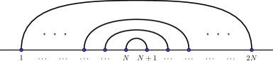
Figure 3.1. The rainbow pattern (planar pair partition) of $2N$ points.

For the special case concerning the rainbow pattern defined by $\boldsymbol{\underline{\Cap}}_{0}=\emptyset$ and

$$\boldsymbol{\underline{\Cap}}_{N}=\left\{\underset{\;1\;\;2N}{\vbox{\hbox{\includegraphics[scale={0.5}]{link-0.pdf}}}},\ldots,\underset{\;N-1\;\;N+2}{\vbox{\hbox{\includegraphics[scale={0.5}]{link-0.pdf}}}},\underset{\;N\;\;N+1}{\vbox{\hbox{\includegraphics[scale={0.5}]{link-0.pdf}}}}\right\}\,\in\,\mathrm{PP}_{N},\quad\text{ for }N\in\mathbb{Z}_{>0},$$

(see also Figure 3.1), the equations (3.13) – (3.15) involve only the rainbow patterns $\boldsymbol{\underline{\Cap}}_{N}$ and $\boldsymbol{\underline{\Cap}}_{N-1}$:

(3.16) $$(K-1).v_{\boldsymbol{\underline{\Cap}}_{N}}=\; 0$$

(3.17) $$E.v_{\boldsymbol{\underline{\Cap}}_{N}}=\; 0$$

(3.18) $$\hat{\pi}^{(1)}_{N}(v_{\boldsymbol{\underline{\Cap}}_{N}})=\; v_{\boldsymbol{\underline{\Cap}}_{N-1}}\qquad\text{and}\qquad\hat{\pi}^{(1)}_{j}(v_{\boldsymbol{\underline{\Cap}}_{N}})=0,\quad\text{for }j\neq N.$$

Therefore, the formula for $v_{\boldsymbol{\underline{\Cap}}_{N}}$ is particularly simple.

Proposition 3.5.

[KP16, Proposition 3.3] The vectors

(3.19) $$v_{\boldsymbol{\underline{\Cap}}_{N}}:=\; \frac{1}{(q^{-2}-1)^{N}}\frac{\left[2\right]^{N}}{\left[N+1\right]!}\,\sum_{l=0}^{N}(-1)^{l}q^{l(N-l-1)}\times\left(\theta_{l}^{(N)}\otimes\theta_{N-l}^{(N)}\right)\,\in\,\mathsf{M}_{2}^{\otimes 2N},$$

for $N\in\mathbb{Z}_{\geq 0}$, determine the unique solution to (3.16) – (3.18) with $v_{\emptyset}=1$.

3.3. Construction

Now we construct the basis vectors $\mathfrak{v}_{\omega}$ of Theorem 3.1. In the construction, we use the vectors $v_{\alpha}$ of Theorem 3.4, with $N=\frac{1}{2}(n+s)$ chosen as in (2.15), and the map (2.16),

$$\mathrm{LP}^{(s)}_{\varsigma}\rightarrow\mathrm{PP}_{N},\qquad\omega\mapsto\alpha(\omega),$$

see also Figure 2.3 in Section 2.6.

For a link pattern $\omega\in\mathrm{LP}^{(s)}_{\varsigma}$, the basis vector $\mathfrak{v}_{\omega}\in\mathsf{H}_{\varsigma}^{(s)}\subset\bigotimes_{i=1}^{p}\mathsf{M}_{d_{i}}$ is obtained from the vector $v_{\alpha(\omega)}\in\mathsf{H}_{2N}^{(0)}\subset\mathsf{M}_{2}^{\otimes 2N}$ as follows: we let

(3.24) $$\mathfrak{v}_{\omega}:=R_{+}^{(s)}\left(\widehat{\mathfrak{p}}^{(\varsigma,s)}(v_{\alpha(\omega)})\right)\qquad\qquad\text{ with }\qquad\qquad\lx@xy@svg{\hbox{\raise 0.0pt\hbox{\kern 14.09253pt\hbox{\ignorespaces\ignorespaces\ignorespaces\hbox{\vtop{\kern 0.0pt\offinterlineskip\halign{\entry@#!@&&\entry@@#!@\cr&&\\&&\crcr}}}\ignorespaces{\hbox{\kern-13.48271pt\raise 0.0pt\hbox{\hbox{\kern 0.0pt\raise 0.0pt\hbox{\hbox{\kern 3.0pt\raise 0.0pt\hbox{$\textstyle{\mathsf{H}_{2N}^{(0)}\;\;\ignorespaces\ignorespaces\ignorespaces\ignorespaces\ignorespaces\ignorespaces\ignorespaces\ignorespaces}$}}}}}}}\ignorespaces\ignorespaces\ignorespaces\ignorespaces{}{\hbox{\lx@xy@droprule}}\ignorespaces\ignorespaces\ignorespaces{\hbox{\kern 22.90004pt\raise 11.66666pt\hbox{{}\hbox{\kern 0.0pt\raise 0.0pt\hbox{\hbox{\kern 3.0pt\hbox{\hbox{\kern 0.0pt\raise-4.36111pt\hbox{$\scriptstyle{\widehat{\mathfrak{p}}^{(\varsigma,s)}}$}}}\kern 3.0pt}}}}}}\ignorespaces{\hbox{\kern 50.09253pt\raise 4.30554pt\hbox{\hbox{\kern 0.0pt\raise 0.0pt\hbox{\lx@xy@tip{1}\lx@xy@tip{-1}}}}}}{\hbox{\lx@xy@droprule}}{\hbox{\lx@xy@droprule}}\ignorespaces\ignorespaces\ignorespaces\ignorespaces{\hbox{\kern 13.48271pt\raise-8.61108pt\hbox{\hbox{\kern 0.0pt\raise 0.0pt\hbox{\lx@xy@tip{1}\lx@xy@tip{-1}}}}}}{\hbox{\lx@xy@droprule}}\ignorespaces\ignorespaces\ignorespaces{\hbox{\kern 24.41394pt\raise-14.75275pt\hbox{{}\hbox{\kern 0.0pt\raise 0.0pt\hbox{\hbox{\kern 3.0pt\hbox{\hbox{\kern 0.0pt\raise-3.14166pt\hbox{$\scriptstyle{\mathfrak{I}^{(\varsigma,s)}}$}}}\kern 3.0pt}}}}}}\ignorespaces{\hbox{\kern 50.09253pt\raise-8.61108pt\hbox{\hbox{\kern 0.0pt\raise 0.0pt\hbox{\lx@xy@hook{-1}}}}}}{\hbox{\lx@xy@droprule}}{\hbox{\lx@xy@droprule}}{\hbox{\kern 50.09253pt\raise 0.0pt\hbox{\hbox{\kern 0.0pt\raise 0.0pt\hbox{\hbox{\kern 3.0pt\raise 0.0pt\hbox{$\textstyle{\;\;\mathsf{H}_{(\varsigma,s)}^{(0)}\ignorespaces\ignorespaces\ignorespaces\ignorespaces}$}}}}}}}\ignorespaces\ignorespaces\ignorespaces\ignorespaces{}{\hbox{\lx@xy@droprule}}\ignorespaces\ignorespaces\ignorespaces{\hbox{\kern 88.84424pt\raise 6.89166pt\hbox{{}\hbox{\kern 0.0pt\raise 0.0pt\hbox{\hbox{\kern 3.0pt\hbox{\hbox{\kern 0.0pt\raise-2.39168pt\hbox{$\scriptstyle{R_{+}^{(s)}}$}}}\kern 3.0pt}}}}}}\ignorespaces{\hbox{\kern 116.72072pt\raise 0.0pt\hbox{\hbox{\kern 0.0pt\raise 0.0pt\hbox{\lx@xy@tip{1}\lx@xy@tip{-1}}}}}}{\hbox{\lx@xy@droprule}}{\hbox{\lx@xy@droprule}}{\hbox{\kern 116.72072pt\raise 0.0pt\hbox{\hbox{\kern 0.0pt\raise 0.0pt\hbox{\hbox{\kern 3.0pt\raise 0.0pt\hbox{$\textstyle{\;\;\mathsf{H}_{\varsigma}^{(s)}}$}}}}}}}{\hbox{\kern-14.09253pt\raise-40.7222pt\hbox{\hbox{\kern 0.0pt\raise 0.0pt\hbox{\hbox{\kern 3.0pt\raise 0.0pt\hbox{$\textstyle{v_{\alpha(\omega)}\;\;\ignorespaces\ignorespaces\ignorespaces\ignorespaces\ignorespaces\ignorespaces\ignorespaces\ignorespaces}$}}}}}}}\ignorespaces\ignorespaces\ignorespaces\ignorespaces{\hbox{\kern 14.09253pt\raise-36.41666pt\hbox{\hbox{\kern 0.0pt\raise 0.0pt\hbox{\lx@xy@stopper}}}}}{\hbox{\lx@xy@droprule}}\ignorespaces\ignorespaces\ignorespaces{\hbox{\kern 22.90004pt\raise-29.05554pt\hbox{{}\hbox{\kern 0.0pt\raise 0.0pt\hbox{\hbox{\kern 3.0pt\hbox{\hbox{\kern 0.0pt\raise-4.36111pt\hbox{$\scriptstyle{\widehat{\mathfrak{p}}^{(\varsigma,s)}}$}}}\kern 3.0pt}}}}}}\ignorespaces{\hbox{\kern 51.96709pt\raise-36.41666pt\hbox{\hbox{\kern 0.0pt\raise 0.0pt\hbox{\lx@xy@tip{1}\lx@xy@tip{-1}}}}}}{\hbox{\lx@xy@droprule}}{\hbox{\lx@xy@droprule}}\ignorespaces\ignorespaces\ignorespaces\ignorespaces{\hbox{\kern 14.09253pt\raise-49.33328pt\hbox{\hbox{\kern 0.0pt\raise 0.0pt\hbox{\lx@xy@tip{1}\lx@xy@tip{-1}}}}}}{\hbox{\lx@xy@droprule}}\ignorespaces\ignorespaces\ignorespaces{\hbox{\kern 24.41394pt\raise-55.47495pt\hbox{{}\hbox{\kern 0.0pt\raise 0.0pt\hbox{\hbox{\kern 3.0pt\hbox{\hbox{\kern 0.0pt\raise-3.14166pt\hbox{$\scriptstyle{\mathfrak{I}^{(\varsigma,s)}}$}}}\kern 3.0pt}}}}}}\ignorespaces{\hbox{\kern 51.96709pt\raise-49.33328pt\hbox{\hbox{\kern 0.0pt\raise 0.0pt\hbox{\lx@xy@hook{-1}}}}}}{\hbox{\lx@xy@droprule}}{\hbox{\lx@xy@droprule}}{\hbox{\kern 51.96709pt\raise-40.7222pt\hbox{\hbox{\kern 0.0pt\raise 0.0pt\hbox{\hbox{\kern 3.0pt\raise 0.0pt\hbox{$\textstyle{\;\;\mathfrak{v}_{\omega}^{\infty}\;\;\ignorespaces\ignorespaces\ignorespaces\ignorespaces}$}}}}}}}\ignorespaces\ignorespaces\ignorespaces\ignorespaces{\hbox{\kern 77.84148pt\raise-40.7222pt\hbox{\hbox{\kern 0.0pt\raise 0.0pt\hbox{\lx@xy@stopper}}}}}{\hbox{\lx@xy@droprule}}\ignorespaces\ignorespaces\ignorespaces{\hbox{\kern 88.84424pt\raise-33.83054pt\hbox{{}\hbox{\kern 0.0pt\raise 0.0pt\hbox{\hbox{\kern 3.0pt\hbox{\hbox{\kern 0.0pt\raise-2.39168pt\hbox{$\scriptstyle{R_{+}^{(s)}}$}}}\kern 3.0pt}}}}}}\ignorespaces{\hbox{\kern 115.71603pt\raise-40.7222pt\hbox{\hbox{\kern 0.0pt\raise 0.0pt\hbox{\lx@xy@tip{1}\lx@xy@tip{-1}}}}}}{\hbox{\lx@xy@droprule}}{\hbox{\lx@xy@droprule}}{\hbox{\kern 115.71603pt\raise-40.7222pt\hbox{\hbox{\kern 0.0pt\raise 0.0pt\hbox{\hbox{\kern 3.0pt\raise 0.0pt\hbox{$\textstyle{\;\;\mathfrak{v}_{\omega},}$}}}}}}}\ignorespaces}}}}\ignorespaces \textstyle{\mathsf{H}_{2N}^{(0)}\;\;\ignorespaces\ignorespaces\ignorespaces\ignorespaces\ignorespaces\ignorespaces\ignorespaces\ignorespaces} \scriptstyle{\widehat{\mathfrak{p}}^{(\varsigma,s)}} \scriptstyle{\mathfrak{I}^{(\varsigma,s)}} \textstyle{\;\;\mathsf{H}_{(\varsigma,s)}^{(0)}\ignorespaces\ignorespaces\ignorespaces\ignorespaces} \scriptstyle{R_{+}^{(s)}} \textstyle{\;\;\mathsf{H}_{\varsigma}^{(s)}} \textstyle{v_{\alpha(\omega)}\;\;\ignorespaces\ignorespaces\ignorespaces\ignorespaces\ignorespaces\ignorespaces\ignorespaces\ignorespaces} \scriptstyle{\widehat{\mathfrak{p}}^{(\varsigma,s)}} \scriptstyle{\mathfrak{I}^{(\varsigma,s)}} \textstyle{\;\;\mathfrak{v}_{\omega}^{\infty}\;\;\ignorespaces\ignorespaces\ignorespaces\ignorespaces} \scriptstyle{R_{+}^{(s)}} \textstyle{\;\;\mathfrak{v}_{\omega},} \textstyle{\mathsf{H}_{2N}^{(0)}\;\;\ignorespaces\ignorespaces\ignorespaces\ignorespaces\ignorespaces\ignorespaces\ignorespaces\ignorespaces} \scriptstyle{\widehat{\mathfrak{p}}^{(\varsigma,s)}} \scriptstyle{\mathfrak{I}^{(\varsigma,s)}} \textstyle{\;\;\mathsf{H}_{(\varsigma,s)}^{(0)}\ignorespaces\ignorespaces\ignorespaces\ignorespaces} \scriptstyle{R_{+}^{(s)}} \textstyle{\;\;\mathsf{H}_{\varsigma}^{(s)}} \textstyle{v_{\alpha(\omega)}\;\;\ignorespaces\ignorespaces\ignorespaces\ignorespaces\ignorespaces\ignorespaces\ignorespaces\ignorespaces} \scriptstyle{\widehat{\mathfrak{p}}^{(\varsigma,s)}} \scriptstyle{\mathfrak{I}^{(\varsigma,s)}} \textstyle{\;\;\mathfrak{v}_{\omega}^{\infty}\;\;\ignorespaces\ignorespaces\ignorespaces\ignorespaces} \scriptstyle{R_{+}^{(s)}} \textstyle{\;\;\mathfrak{v}_{\omega},}$$

where

• $\widehat{\mathfrak{p}}^{(\varsigma,s)}:=\widehat{\mathfrak{p}}^{(s)}\otimes\widehat{\mathfrak{p}}^{(s_{p})}\otimes\cdots\otimes\widehat{\mathfrak{p}}^{(s_{1})}$ and $\mathfrak{I}^{(\varsigma,s)}:=\mathfrak{I}^{(s)}\otimes\mathfrak{I}^{(s_{p})}\otimes\cdots\otimes\mathfrak{I}^{(s_{1})}$ (recall Section 3.1),

• we denote by $\mathfrak{v}_{\omega}^{\infty}:=\widehat{\mathfrak{p}}^{(\varsigma,s)}(v_{\alpha(\omega)})$, and

• $R_{+}^{(s)}\colon\mathsf{H}_{(\varsigma,s)}^{(0)}\to\mathsf{H}_{\varsigma}^{(s)}$ is a linear isomorphism, which will be defined in more detail in Section 3.4.

The idea is to think the tensor power $\mathsf{M}_{2}^{\otimes 2N}$ of as a chain of blocks of smaller tensor powers of $\mathsf{M}_{2}$,

$$\mathsf{M}_{2}^{\otimes 2N}=\mathsf{M}_{2}^{\otimes s}\otimes\mathsf{M}_{2}^{\otimes s_{p}}\otimes\mathsf{M}_{2}^{\otimes s_{p-1}}\otimes\cdots\otimes\mathsf{M}_{2}^{\otimes s_{2}}\otimes\mathsf{M}_{2}^{\otimes s_{1}},$$

where each block $\mathsf{M}_{2}^{\otimes r}$ is mapped onto the $\delta=r+1$-dimensional irreducible representation $\mathsf{M}_{\delta}$ under the map $\widehat{\mathfrak{p}}^{(\varsigma,s)}\colon\mathsf{M}_{2}^{\otimes 2N}\to\mathsf{M}_{d}\otimes\mathsf{M}_{d_{p}}\otimes\cdots\otimes\mathsf{M}_{d_{1}}$. Conversely, the image of the embedding $\mathfrak{I}^{(\varsigma,s)}$ can be characterized by projection properties inside the blocks, as we show next.

Proposition 3.6.

The image of the space $\mathsf{H}_{(\varsigma,s)}^{(0)}$ under the embedding $\mathfrak{I}^{(\varsigma,s)}$ is the space

$$\mathsf{J}^{(\varsigma,s)}_{N}:=\left\{v\in\mathsf{H}_{2N}^{(0)}\;\Big{|}\;\hat{\pi}^{(1)}_{j}(v)=0,\text{ for all }j\in\big{\{}1,\ldots,2N-1\big{\}}\setminus\bigg{\{}\sum_{i=1}^{k}s_{i}\;\big{|}\;1\leq k\leq p\bigg{\}}\right\}.$$

The projection $\widehat{\mathfrak{p}}^{(\varsigma,s)}$ defines an isomorphism of representations of $\mathcal{U}_{q}(\mathfrak{sl}_{2})$,

$$\widehat{\mathfrak{p}}^{(\varsigma,s)}\;\colon\;\mathsf{J}^{(\varsigma,s)}_{N}\to\mathsf{H}_{(\varsigma,s)}^{(0)},$$

and its inverse is $\mathfrak{I}^{(\varsigma,s)}$. For any $\omega\in\mathrm{LP}^{(s)}_{\varsigma}$, the vector $v_{\alpha(\omega)}$ lies in the space $\mathsf{J}^{(\varsigma,s)}_{N}$ and, in particular,

(3.25) $$\mathfrak{I}^{(\varsigma,s)}\left(\widehat{\mathfrak{p}}^{(\varsigma,s)}(v_{\alpha(\omega)})\right)=\mathfrak{I}^{(\varsigma,s)}\left(\mathfrak{v}_{\omega}^{\infty}\right)=v_{\alpha(\omega)}.$$

Proof.

The property $\mathfrak{I}^{(\varsigma,s)}\big{(}\mathsf{H}_{(\varsigma,s)}^{(0)}\big{)}=\mathsf{J}^{(\varsigma,s)}_{N}$ follows from Lemma 3.3 and the fact that $\mathfrak{I}^{(\varsigma,s)}$ commutes with the action of the algebra $\mathcal{U}_{q}(\mathfrak{sl}_{2})$. Since $\widehat{\mathfrak{p}}^{(\varsigma,s)}$ also commutes with the action of $\mathcal{U}_{q}(\mathfrak{sl}_{2})$, it follows that restricted to $\mathsf{J}^{(\varsigma,s)}_{N}$, it is an isomorphism of representations, with inverse $\mathfrak{I}^{(\varsigma,s)}$.

Let then $\omega\in\mathrm{LP}^{(s)}_{\varsigma}$. By definition of the map $\omega\mapsto\alpha(\omega)$ in Section 2.6, the planar pair partition $\alpha(\omega)$ can contain a link of type $\underset{\;\boldsymbol{j}\;\;\boldsymbol{j+1}}{\vbox{\hbox{\includegraphics[scale={0.5}]{link-0.pdf}}}}$ only if these points correspond to different points in the link pattern $\omega$, that is, if $j\in\left\{\sum_{i=1}^{k}s_{i}\;\big{|}\;1\leq k\leq p\right\}$. In particular, by the projection properties (3.15) of $v_{\alpha(\omega)}$, we have $\hat{\pi}^{(1)}_{j}(v_{\alpha(\omega)})=0$, for all $j\notin\left\{\sum_{i=1}^{k}s_{i}\;\big{|}\;1\leq k\leq p\right\}$, so $v_{\alpha(\omega)}\in\mathsf{J}^{(\varsigma,s)}_{N}$. This concludes the proof. ∎

It now follows almost immediately from the definitions that the vectors (3.24) form a basis of the highest weight vector space. This proves part (b) of Theorem 3.1.

Proposition 3.7.

The collection $\left(\mathfrak{v}_{\omega}\right)_{\omega\in\mathrm{LP}^{(s)}_{\varsigma}}$ defined in (3.24) is a basis of the vector space $\mathsf{H}_{\varsigma}^{(s)}$.

Proof.

Because $R_{+}^{(s)}\colon\mathsf{H}_{(\varsigma,s)}^{(0)}\to\mathsf{H}_{\varsigma}^{(s)}$ is a linear isomorphism (by [KP20, Lemma 5.3]), the vectors $\mathfrak{v}_{\omega}:=R_{+}^{(s)}\left(\widehat{\mathfrak{p}}^{(\varsigma,s)}(v_{\alpha(\omega)})\right)$ belong to the space $\mathsf{H}_{\varsigma}^{(s)}$ by construction. Their linear independence follows the facts that, first, the maps $R_{+}^{(s)}$ and $\widehat{\mathfrak{p}}^{(\varsigma,s)}$ are linear isomorphisms, by [KP20, Lemma 5.3(a)] and Proposition 3.6, respectively, and second, the vectors $v_{\alpha(\omega)}$ are linearly independent, by Theorem 3.4. Finally, by Lemma 2.2, the linear span of the vectors $\mathfrak{v}_{\omega}$, for $\omega\in\mathrm{LP}^{(s)}_{\varsigma}$, has the correct dimension $\#\mathrm{LP}^{(s)}_{\varsigma}=\mathrm{dim}\mathsf{H}_{\varsigma}^{(s)}$. ∎

To prove part (a) of Theorem 3.1, we still have to show that the vectors $\mathfrak{v}_{\omega}$ satisfy (3.3) – (3.11). The projection properties (3.3) will be verified in Section 3.5. The normalization conditions (3.11) follow by considering the action of the map $R_{+}^{(s)}$ on the vectors $v_{\boldsymbol{\underline{\Cap}}_{s}}$, associated to the rainbow link patterns $\boldsymbol{\underline{\Cap}}_{s}$.

3.4. Normalization

For any partition $\lambda$ of $s$, the vectors $\mathfrak{v}_{\shuffle_{\lambda}}$ correspond to $v_{\boldsymbol{\underline{\Cap}}_{N}}$ with $N=s$ under the map $\omega\mapsto\alpha(\omega)$ — see Figure 3.2 for an illustration. This observation gives rise to the normalization constant in (3.11), as we show next.

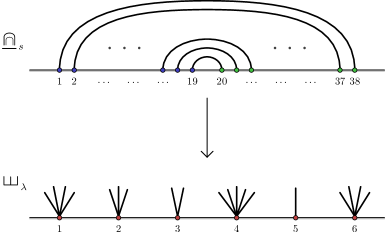
Figure 3.2. For the link pattern $\shuffle_{\lambda}$, consisting of $s$ defects, the corresponding planar pair partition $\alpha(\shuffle_{\lambda})$ is the rainbow pattern $\boldsymbol{\underline{\Cap}}_{s}=\alpha(\shuffle_{\lambda})$.

First, we give the precise definition of the linear isomorphism $R_{+}^{(s)}$ already used above in Equation (3.24). By [KP20, Lemma 5.3(a)], any vector $v\in\mathsf{H}_{(\varsigma,s)}^{(0)}$ can be written in the form

$$v=\sum_{l=0}^{s}(-1)^{s-l}q^{(l+1)(s-l)}\times(e_{l}^{(d)}\otimes F^{s-l}.\tau_{0}^{+}),$$

for a unique vector $\tau_{0}^{+}\in\mathsf{H}_{\varsigma}^{(s)}$, with $d=s+1$. The map (compare with $\mathcal{R}_{+}^{(s)}$ in Section 2.6)

(3.26) $$R_{+}=R_{+}^{(s)}\;\colon\;\mathsf{H}_{(\varsigma,s)}^{(0)}\to\mathsf{H}_{\varsigma}^{(s)},\qquad\qquad R_{+}^{(s)}(v):=\tau_{0}^{+},$$

is thus well-defined. It was shown in [KP20, Lemma 5.3] that $R_{+}^{(s)}$ is a linear isomorphism.

Remark 3.8.

The map $R_{+}^{(s)}$ commutes with the maps $\widetilde{\pi}_{j}^{(\delta)}$ defined in (2.12), for any $j\in\{1,2,\ldots,p-1\}$, $m\in\{0,1,\ldots,\min(s_{j},s_{j+1})\}$, and $\delta=s_{j}+s_{j+1}+1-2m$, because the maps $\widetilde{\pi}_{j}^{(\delta)}$ act on the tensor components $(j,j+1)$ of the tensor product $\mathsf{M}_{d}\otimes\mathsf{M}_{d_{p}}\otimes\mathsf{M}_{d_{p-1}}\otimes\cdots\otimes\mathsf{M}_{d_{2}}\otimes\mathsf{M}_{d_{1}}$, away from the tensor position involving $\mathsf{M}_{d}$ — see also [KP20, Lemma 5.3 & Equation (5.2)].

Lemma 3.9.

Let $\lambda=(s_{1},\ldots,s_{|\lambda|})$ be a partition of $s\in\mathbb{Z}_{>0}$. Then we have $\alpha(\shuffle_{\lambda})=\boldsymbol{\underline{\Cap}}_{s}$, and

$$\mathfrak{v}_{\shuffle_{\lambda}}:=R_{+}^{(s)}\left(\widehat{\mathfrak{p}}^{(\lambda,s)}(v_{\boldsymbol{\underline{\Cap}}_{s}})\right)=\frac{1}{(q-q^{-1})^{s}}\frac{\left[2\right]^{s}}{\left[s+1\right]!}\times(e_{0}^{(s_{|\lambda|}+1)}\otimes\cdots\otimes e_{0}^{(s_{1}+1)})\,\in\,\mathsf{H}_{\lambda}^{(s)}.$$

Proof.

The first assertion $\alpha(\shuffle_{\lambda})=\boldsymbol{\underline{\Cap}}_{s}$ is immediate from the definition of the map $\omega\mapsto\alpha(\omega)$. For the second assertion, using the formula (3.19) for the vector $v_{\boldsymbol{\underline{\Cap}}_{s}}$, we calculate the image of $v_{\boldsymbol{\underline{\Cap}}_{s}}$ under the map $\widehat{\mathfrak{p}}^{(\lambda,s)}=\widehat{\mathfrak{p}}^{(s)}\otimes\widehat{\mathfrak{p}}^{\lambda}=\widehat{\mathfrak{p}}^{(s)}\otimes(\widehat{\mathfrak{p}}^{(s_{|\lambda|})}\otimes\cdots\otimes\widehat{\mathfrak{p}}^{(s_{1})})$:

$$\widehat{\mathfrak{p}}^{(\lambda,s)}(v_{\boldsymbol{\underline{\Cap}}_{s}})=\; \frac{1}{(q^{-2}-1)^{s}}\frac{\left[2\right]^{s}}{\left[s+1\right]!}\,\sum_{l=0}^{s}(-1)^{l}q^{l(s-l-1)}\times\left(\widehat{\mathfrak{p}}^{(s)}(\theta_{l}^{(s)})\otimes\widehat{\mathfrak{p}}^{\lambda}(\theta_{s-l}^{(s)})\right)$$

$$=\; \frac{1}{(q^{-2}-1)^{s}}\frac{\left[2\right]^{s}}{\left[s+1\right]!}\,\sum_{l=0}^{s}(-1)^{l}q^{l(s-l-1)}\times\left(e_{l}^{(d)}\otimes F^{s-l}.(e_{0}^{(s_{|\lambda|}+1)}\otimes\cdots\otimes e_{0}^{(s_{1}+1)})\right).$$

The second assertion now follows from the definition of the map $R_{+}^{(s)}$ in (3.26). ∎

3.5. Projection properties

We show next that the vectors $\mathfrak{v}_{\omega}$ defined by (3.24) indeed satisfy the projection properties (3.3). To establish this, we need some auxiliary calculations, given in Appendix B. The crucial observation is the following commutative diagram.

Lemma 3.10.

Let $s_{1},s_{2}\in\mathbb{Z}_{>0}$ and $m\in\{1,2,\ldots,\min(s_{1},s_{2})\}$, and denote $r=s_{1}+s_{2}-2m$ and $\delta=r+1$. The following diagram commutes, up to a non-zero multiplicative constant, given below.

More precisely, we have

$$\widehat{\mathfrak{p}}^{(r)}\circ\left(\hat{\pi}^{(1)}_{s_{1}-m+1}\circ\cdots\circ\hat{\pi}^{(1)}_{s_{1}-1}\circ\hat{\pi}^{(1)}_{s_{1}}\right)\circ\left(\mathfrak{I}^{(s_{2})}\otimes\mathfrak{I}^{(s_{1})}\right)= \;\mathcal{C}({m;s_{1},s_{2}})\times\hat{\pi}^{(\delta)},$$

where the non-zero constant equals

$$\mathcal{C}({m;s_{1},s_{2}})=\frac{\left[s_{1}-m\right]!\left[s_{2}-m\right]!\left[s_{1}+s_{2}-m+1\right]!}{\left[2\right]^{m}\left[s_{1}\right]!\left[s_{2}\right]!\left[s_{1}+s_{2}-2m+1\right]!}=\frac{\left[\begin{array}[]{c}s_{1}+s_{2}-m+1\\ m\end{array}\right]}{\left[2\right]^{m}\left[m\right]!\left[\begin{array}[]{c}s_{1}\\ m\end{array}\right]\left[\begin{array}[]{c}s_{2}\\ m\end{array}\right]}.$$

Proof.

The subrepresentation isomorphic to $\mathsf{M}_{\delta}$ appears in the tensor product $\mathsf{M}_{d_{2}}\otimes\mathsf{M}_{d_{1}}$ with multiplicity one. By Schur’s lemma, to prove that the diagram commutes, it therefore suffices to show that the map $\widehat{\mathfrak{p}}^{(r)}\circ\left(\hat{\pi}^{(1)}_{s_{1}-m+1}\circ\cdots\circ\hat{\pi}^{(1)}_{s_{1}-1}\circ\hat{\pi}^{(1)}_{s_{1}}\right)\circ\left(\mathfrak{I}^{(s_{2})}\otimes\mathfrak{I}^{(s_{1})}\right)$ is non-zero. But, by Lemma B.5, the vector $\tau_{0}^{(\delta;d_{1},d_{2})}\in\mathsf{M}_{d_{2}}\otimes\mathsf{M}_{d_{1}}$ maps to a non-zero multiple of $e_{0}^{(\delta)}\in\mathsf{M}_{\delta}$ in this map, with the explicit, non-zero proportionality constant $\mathcal{C}({m;s_{1},s_{2}})$. This finishes the proof. ∎

Proposition 3.11.

The collection of vectors $\left(\mathfrak{v}_{\omega}\right)_{\omega\in\mathrm{LP}^{(s)}}$, defined in (3.24), satisfies the equations (3.3).

Proof.

By Remark 3.8, the maps $\tilde{\pi}_{j}^{(\delta)}$ appearing in the equations (3.3) commute with the linear isomorphism $R_{+}^{(s)}$, for any $j\in\{1,2,\ldots,p-1\}$, $m\in\{0,1,\ldots,\min(s_{j},s_{j+1})\}$, and $\delta=s_{j}+s_{j+1}+1-2m$. Therefore, it suffices to show that the vector $\mathfrak{v}_{\omega}^{\infty}:=\widehat{\mathfrak{p}}^{(\varsigma,s)}(v_{\alpha(\omega)})$ satisfies the properties (3.3). Using the commutative diagram of Lemma 3.10 together with Proposition 3.6, the properties (3.3) can be written in terms of $v_{\alpha(\omega)}$, which, in turn, are known to satisfy the properties (3.15), by Theorem 3.4.

Fix $j\in\{1,2,\ldots,p-1\}$, $m\in\{1,2,\ldots,\min(s_{j},s_{j+1})\}$, and denote by $k_{j}=\sum_{i=1}^{j}s_{i}$. We first note that, by definition of the map $\omega\to\alpha(\omega)$ (see Section 2.6), the link pattern $\alpha(\omega)$ contains the nested links

$$\underset{\;k_{j}\;\;k_{j}+1}{\vbox{\hbox{\includegraphics[scale={0.5}]{link-0.pdf}}}},\underset{\;k_{j}-1\;\;k_{j}+2}{\vbox{\hbox{\includegraphics[scale={0.5}]{link-0.pdf}}}},\ldots,\underset{\;k_{j}-m+1\;\;k_{j}+m}{\vbox{\hbox{\includegraphics[scale={0.5}]{link-0.pdf}}}}$$

if and only if the link pattern $\omega$ contains at least $m$ links $\underset{\;\boldsymbol{j}\;\;\boldsymbol{j+1}}{\vbox{\hbox{\includegraphics[scale={0.5}]{link-0.pdf}}}}$ , and if this is the case, then we have

$$\alpha(\omega)\;/\underset{\;k_{j}\;\;k_{j}+1}{\vbox{\hbox{\includegraphics[scale={0.5}]{link-0.pdf}}}}\;/\underset{\;k_{j}-1\;\;k_{j}+2}{\vbox{\hbox{\includegraphics[scale={0.5}]{link-0.pdf}}}}\;/\;\ldots\;/\underset{\;k_{j}-m+1\;\;k_{j}+m}{\vbox{\hbox{\includegraphics[scale={0.5}]{link-0.pdf}}}}=\; \alpha\Big{(}\omega/(m\times\underset{\;j\;\;j+1}{\vbox{\hbox{\includegraphics[scale={0.5}]{link-0.pdf}}}})\Big{)}=\alpha(\hat{\omega}),$$

where we denote by $\hat{\omega}=\omega/(m\times\raisebox{2.15277pt}{ \scalebox{0.75}{$\underset{\;\boldsymbol{j}\;\;\boldsymbol{j+1}}{\vbox{\hbox{\includegraphics[scale={0.5}]{link-0.pdf}}}}$}})$. The projection properties (3.15) for the vector $v_{\alpha(\omega)}$ show that

(3.27) $$\left(\hat{\pi}_{k_{j}-m+1}^{(1)}\circ\cdots\circ\hat{\pi}_{k_{j}-1}^{(1)}\circ\hat{\pi}_{k_{j}}^{(1)}\right)(v_{\alpha(\omega)})=\; \begin{cases}v_{\alpha(\hat{\omega})}&\mbox{if there are at least $m$ links }\underset{\;j\;\;j+1}{\vbox{\hbox{\includegraphics[scale={0.5}]{link-0.pdf}}}}\text{ in }\omega\\ 0&\mbox{otherwise}.\end{cases}$$

Denote by $r=\delta-1=s_{j}+s_{j+1}-2m$ and $\hat{\varsigma}=(s_{1},\ldots,s_{j-1},r,s_{j+2},\ldots,s_{p})$. Using the commutative diagram of Lemma 3.10, Equation (3.25), and Equation (3.27), we obtain

(3.28) $$\mathcal{C}({m;s_{j},s_{j+1}})\times\hat{\pi}_{j}^{(\delta)}(\mathfrak{v}_{\omega}^{\infty})=\; \left(\widehat{\mathfrak{p}}^{(\hat{\varsigma},s)}\circ\left(\hat{\pi}_{k_{j}-m+1}^{(1)}\circ\cdots\circ\hat{\pi}_{k_{j}-1}^{(1)}\circ\hat{\pi}_{k_{j}}^{(1)}\right)\circ\mathfrak{I}^{(\varsigma,s)}\right)(\mathfrak{v}_{\omega}^{\infty})$$

$$=\; \left(\widehat{\mathfrak{p}}^{(\hat{\varsigma},s)}\circ\left(\hat{\pi}_{k_{j}-m+1}^{(1)}\circ\cdots\circ\hat{\pi}_{k_{j}-1}^{(1)}\circ\hat{\pi}_{k_{j}}^{(1)}\right)\right)(v_{\alpha(\omega)})$$

$$=\; \begin{cases}\widehat{\mathfrak{p}}^{(\hat{\varsigma},s)}(v_{\alpha(\hat{\omega})})&\mbox{if there are at least $m$ links }\underset{\;j\;\;j+1}{\vbox{\hbox{\includegraphics[scale={0.5}]{link-0.pdf}}}}\text{ in }\omega\\ 0&\mbox{otherwise}.\end{cases}$$

Now, it follows directly from the definitions that we have

(3.29) $$\widehat{\mathfrak{p}}^{(s_{j+1}-m)}\otimes\widehat{\mathfrak{p}}^{(s_{j}-m)}=\iota^{(\delta)}\circ\widehat{\mathfrak{p}}^{(r)}\;\colon\;\mathsf{M}_{2}^{\otimes r}\to\mathsf{M}_{d_{j+1}-m}\otimes\mathsf{M}_{d_{j}-m},$$

where the maps $\widehat{\mathfrak{p}}^{(r)}\colon\mathsf{M}_{2}^{\otimes r}\to\mathsf{M}_{\delta}$ and $\iota^{(\delta)}=\iota^{(\delta;d_{j}-m,d_{j+1}-m)}\colon\mathsf{M}_{\delta}\hookrightarrow\mathsf{M}_{d_{j+1}-m}\otimes\mathsf{M}_{d_{j}-m}$ were defined in (3.12) and (2.9), respectively. Using Equation (2.12), Equation (3.28), and Equation (3.29), we obtain

$$\mathcal{C}({m;s_{j},s_{j+1}})\times\tilde{\pi}_{j}^{(\delta)}(\mathfrak{v}_{\omega}^{\infty})=\; \mathcal{C}({m;s_{j},s_{j+1}})\times\iota_{j}^{(\delta)}\left(\hat{\pi}_{j}^{(\delta)}(\mathfrak{v}_{\omega}^{\infty})\right)$$

$$=\; \begin{cases}\left(\iota_{j}^{(\delta)}\circ\widehat{\mathfrak{p}}^{(\hat{\varsigma},s)}\right)(v_{\alpha(\hat{\omega})})&\mbox{if there are at least $m$ links }\underset{\;j\;\;j+1}{\vbox{\hbox{\includegraphics[scale={0.5}]{link-0.pdf}}}}\text{ in }\omega\\ 0&\mbox{otherwise}\end{cases}$$

$$=\; \begin{cases}\widehat{\mathfrak{p}}^{(\tilde{\varsigma},s)}(v_{\alpha(\hat{\omega})})&\mbox{if there are at least $m$ links }\underset{\;j\;\;j+1}{\vbox{\hbox{\includegraphics[scale={0.5}]{link-0.pdf}}}}\text{ in }\omega\\ 0&\mbox{otherwise}\end{cases}$$

$$=\; \begin{cases}\mathfrak{v}_{\hat{\omega}}^{\infty}&\mbox{if there are at least $m$ links }\underset{\;j\;\;j+1}{\vbox{\hbox{\includegraphics[scale={0.5}]{link-0.pdf}}}}\text{ in }\omega\\ 0&\mbox{otherwise},\end{cases}$$

where $\tilde{\varsigma}=(s_{1},\ldots,s_{j-1},s_{j}-m,s_{j+1}-m,s_{j+2},\ldots,s_{p})$, and $\mathfrak{v}_{\hat{\omega}}^{\infty}=\widehat{\mathfrak{p}}^{(\tilde{\varsigma},s)}(v_{\alpha(\hat{\omega})})$. This is the property (3.3) for $\mathfrak{v}_{\omega}^{\infty}$. Finally, we obtain the asserted property for $\mathfrak{v}_{\omega}$ by applying the map $R_{+}^{(s)}$:

$$\tilde{\pi}_{j}^{(\delta)}(\mathfrak{v}_{\omega})=\; \begin{cases}\frac{1}{\mathcal{C}({m;s_{j},s_{j+1}})}\times\mathfrak{v}_{\hat{\omega}}&\mbox{if there are at least $m$ links }\underset{\;j\;\;j+1}{\vbox{\hbox{\includegraphics[scale={0.5}]{link-0.pdf}}}}\text{ in }\omega\\ 0&\mbox{otherwise}.\end{cases}$$

∎

3.6. Uniqueness

We finish by proving that the solutions to (3.1) – (3.3) are necessarily unique, up to normalization. Fixing the normalization (3.11), uniqueness follows from the observation that the homogeneous system, in which all of the projections vanish, admits a non-trivial solution only when $n=\sum_{i=1}^{p}s_{i}=s$, and in this case, the space $\mathsf{H}_{\varsigma}^{(s)}$ is one-dimensional and spanned by $\mathfrak{v}_{\shuffle_{\varsigma}}$ (see Remark 3.2).

Lemma 3.12.

Assume that $n>s$ and that the vector $v\in\bigotimes_{i=1}^{p}\mathsf{M}_{d_{i}}$ satisfies $E.v=0$, $K.v=q^{s}\,v$, and $\widetilde{\pi}_{j}^{(\delta)}(v)=0$, for all $j\in\{1,2,\ldots,p-1\}$, all $\delta=s_{j}+s_{j+1}+1-2m$, and all $m\in\{1,2,\ldots,\min(s_{j+1},s_{j})\}$. Then we have $v=0.$

Proof.

The properties $E.v=0$ and $K.v=q^{s}\,v$ show that $v$ belongs to the highest weight vector space $\mathsf{H}_{\varsigma}^{(s)}$, so we have $\mathfrak{I}^{(\varsigma)}(v)=(\mathfrak{I}^{(s_{p})}\otimes\cdots\otimes\mathfrak{I}^{(s_{1})})(v)\in\mathsf{H}_{n}^{(s)}$ as well. Furthermore, the properties $\widetilde{\pi}_{j}^{(\delta)}(v)=0$, for all $j$, $\delta$, and $m$ imply that in the tensor product (2.5), in the direct sum decomposition of any two consecutive tensorands $\mathsf{M}_{d_{j+1}}\otimes\mathsf{M}_{d_{j}}$ into irreducibles, the vector $v$ lies in the highest dimensional subrepresentation isomorphic to $\mathsf{M}_{d_{j}+d_{j+1}-1}$. For the vector $\mathfrak{I}^{(\varsigma)}(v)$, this and Lemma 3.3 show that we have

$$\hat{\pi}^{(1)}_{k}\left(\mathfrak{I}^{(\varsigma)}(v)\right)=0,\qquad\text{for all }\;k\in\{1,2,\ldots,n-1\}.$$

Therefore, Lemma 3.3 applied to the whole tensor product $\mathsf{M}_{2}^{\otimes n}$ shows that the vector $\mathfrak{I}^{(\varsigma)}(v)$ belongs to the highest dimensional subrepresentation $\mathsf{M}_{n+1}\subset\mathsf{M}_{2}^{\otimes n}$. We conclude that

$$\mathfrak{I}^{(\varsigma)}(v)\in\mathsf{M}_{s+1}\cap\mathsf{M}_{n+1}\subset\mathsf{M}_{2}^{\otimes n}.$$

Now, by assumption $n>s$, we have $\mathsf{M}_{s+1}\cap\mathsf{M}_{n+1}=\left\{0\right\}$, so we get $\mathfrak{I}^{(\varsigma)}(v)=0$, and $v=0$ as well. ∎

Proposition 3.13.

Let $s\in\mathbb{Z}_{\geq 0}$, and let $\left(\mathfrak{v}_{\omega}\right)_{\omega\in\mathrm{LP}^{(s)}}$ and $\left(\mathfrak{v}^{\prime}_{\omega}\right)_{\omega\in\mathrm{LP}^{(s)}}$ be two collections of solutions to (3.1) – (3.3), such that we have $\mathfrak{v}_{\shuffle_{\lambda}},\mathfrak{v}_{\shuffle_{\lambda}}^{\prime}\neq 0$, for all partitions $\lambda$ of $s$. Then, there are constants $c_{\lambda}\in\mathbb{C}\setminus\{0\}$ such that

$$\mathfrak{v}^{\prime}_{\omega}=c_{\lambda}\,\mathfrak{v}_{\omega},\qquad\text{for all }\omega\in\mathrm{LP}^{(s)}(\lambda).$$

Proof.

Fix a partition $\lambda$ of $s$. By assumption, we have $\mathfrak{v}_{\shuffle_{\lambda}}^{\prime}=c_{\lambda}\,\mathfrak{v}_{\shuffle_{\lambda}}$, for some $c_{\lambda}\in\mathbb{C}\setminus\{0\}$, because the vectors $\mathfrak{v}_{\shuffle_{\lambda}}^{\prime}$ and $\mathfrak{v}_{\shuffle_{\lambda}}$ belong to a one-dimensional space (see Remark 3.2). Suppose then that the condition $\mathfrak{v}^{\prime}=c_{\lambda}\,\mathfrak{v}_{\tau}$ holds for all $\tau\in\mathrm{LP}^{(s)}(\lambda)\cap\mathrm{LP}_{\varrho}^{(s)}$ for which the multiindex $\varrho=(r_{1},\ldots,r_{t})$ satisfies $\sum_{i=1}^{t}r_{i}=n\geq s$. Then, for any $\omega\in\mathrm{LP}^{(s)}(\lambda)\cap\mathrm{LP}_{\varsigma}^{(s)}$ with $\varsigma=(s_{1},\ldots,s_{p})$ such that $\sum_{i=1}^{p}s_{i}=n+1$, the equations (3.1) – (3.3) for $\mathfrak{v}_{\omega}^{\prime}$ and $c_{\lambda}\,\mathfrak{v}_{\omega}$ coincide. It thus follows from Lemma 3.12 that we have $\mathfrak{v}_{\omega}^{\prime}=c_{\lambda}\,\mathfrak{v}_{\omega}$, for all $\omega\in\mathrm{LP}^{(s)}(\lambda)\cap\mathrm{LP}_{\varsigma}^{(s)}$. The assertion then follows by induction on $n$. ∎

3.7. Proof of Theorem 3.1

For $\omega\in\mathrm{LP}^{(s)}$, the vectors $\mathfrak{v}_{\omega}$ defined in Equation (3.24) are solutions to (3.1) – (3.3); see Proposition 3.7 for the conditions (3.1) and (3.2), and Proposition 3.11 for (3.3). By Lemma 3.9, the vectors $\mathfrak{v}_{\shuffle_{\lambda}}$ satisfy the asserted normalization (3.11), for all partitions $\lambda$ of $s$. Uniqueness of the solutions follows from Proposition 3.13. This proves part (a). Part (b) follows from Proposition 3.7. This concludes the proof of Theorem 3.1. $\hfill\qed$

4. Cyclic permutation symmetry of the basis vectors

Next, we derive a further property of the basis vectors $\mathfrak{v}_{\omega}$, also very natural in terms of the link patterns $\omega$. This is a symmetry property under cyclic permutations of the tensor components $\mathsf{M}_{d_{i}}$ in the trivial subrepresentation $\mathsf{H}_{\varsigma}^{(0)}\subset\bigotimes_{i=1}^{p}\mathsf{M}_{d_{i}}$. We show in Corollary 4.2 that under such a cyclic permutation, the vectors $\mathfrak{v}_{\omega}\in\mathsf{H}_{\varsigma}^{(0)}$, with $\varsigma=(s_{1},\ldots,s_{p})$, are mapped to constant multiples of similar vectors $\mathfrak{v}_{\omega^{\prime}}\in\mathsf{H}^{(0)}_{\varsigma^{\prime}}$, where the link pattern $\omega^{\prime}\in\mathrm{LP}^{(0)}_{\varsigma^{\prime}}$ is obtained by applying the combinatorial bijections $\mathcal{R}_{+}$ and $\mathcal{R}_{-}$ of Section 2.6, so that we either have $\varsigma^{\prime}=(s_{p},s_{1},s_{2},\ldots,s_{p-1})$ or $\varsigma^{\prime}=(s_{2},s_{3},\ldots,s_{p},s_{1})$, depending on the orientation of the permutation — see Figure 4.1 for an illustration of the former case. From this property, it also follows (Corollary 4.3) that the $p$:th iterate of the cyclic permutation of the tensor components is a constant multiple of the identity map on $\mathsf{H}_{\varsigma}^{(0)}$.

4.1. Placing tensor components at infinity

We now consider the linear isomorphism $R_{+}$ defined in Section 3.4, and a similar linear isomorphism

(4.1) $$R_{-}=R_{-}^{(s)}\;\colon\;\mathsf{H}_{(s,\varsigma)}^{(0)}\to\mathsf{H}_{\varsigma}^{(s)},\qquad\qquad R_{-}^{(s)}(v):=\tau_{0}^{-},$$

where $\tau_{0}^{-}\in\mathsf{H}_{\varsigma}^{(s)}$ is the unique vector such that we have

$$v=\sum_{l=0}^{s}(-1)^{s-l}q^{(l-1)(s-l)}\times(F^{s-l}.\tau_{0}^{-}\otimes e_{l}^{(d)}),$$

with $d=s+1$; see [KP20, Lemma 5.3] (compare also with $\mathcal{R}_{+}$ and $\mathcal{R}_{-}$ in Section 2.6).

We also define the composed map $S=R_{-}^{-1}\circ R_{+}$, permuting the tensor components cyclically,

(4.2) $$S=S^{(s)}\;\colon\;\mathsf{H}_{(\varsigma,s)}^{(0)}\to\mathsf{H}_{(s,\varsigma)}^{(0)}.$$

Iterating the map $S$, we define a linear map on $\mathsf{H}_{\varsigma}^{(0)}$, with $\varsigma=(s_{1},\ldots,s_{p})$,

(4.3) $$S^{(s_{1})}\circ S^{(s_{2})}\circ\cdots\circ S^{(s_{p-1})}\circ S^{(s_{p})}\;\colon\;\mathsf{H}_{\varsigma}^{(0)}\to\mathsf{H}_{\varsigma}^{(0)}.$$

Analogously to the map (4.2), we denote the composition of the maps defined in Section 2.6 by

(4.4) $$\mathcal{S}=\mathcal{S}^{(s)}\;\colon\;\mathrm{LP}^{(0)}_{(\varsigma,s)}\to\mathrm{LP}^{(0)}_{(s,\varsigma)},\qquad\mathcal{S}:=\mathcal{R}_{-}^{-1}\circ\mathcal{R}_{+}.$$

When $\varsigma=(s_{1},\ldots,s_{p})$, the link pattern $\mathcal{S}(\omega)$ is obtained from $\omega\in\mathrm{LP}^{(0)}_{(\varsigma,s)}$ by moving the rightmost index $p+1$ of $\omega$ (with valence $s$) to the left of all others, and relabeling the indices from left to right by $1,2,3,\ldots,p+1$. This is illustrated in Figure 4.1.

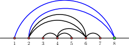
$\mapsto$   

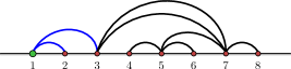
Figure 4.1. In the cyclic permutation $\mathcal{S}=\mathcal{R}_{-}^{-1}\circ\mathcal{R}_{+}$, the rightmost point $p+1=8$ is moved to the left of all others, and the points are relabeled by $1,2,\ldots,8$.

4.2. Cyclic permutations of tensor components

In Section 3.3, we constructed the vectors $\mathfrak{v}_{\omega}$ using the map $R_{+}$, see (3.24). It follows from Proposition 3.13 below that the construction could have been established as well using the map $R_{-}$ instead, only changing the normalization (3.11) of $\mathfrak{v}_{\omega}$.

Let $N$ be chosen as in (2.15) and recall the map $\omega\mapsto\alpha(\omega)$ from Section 2.6, illustrated in Figure 2.3. For convenience, we denote the $s$:th iterate of the map $\mathcal{S}^{(1)}\colon\mathrm{PP}_{N}\to\mathrm{PP}_{N}$ by $\mathcal{S}^{\circ s}=\mathcal{S}^{(1)}\circ\cdots\circ\mathcal{S}^{(1)}$. We then define, for any $\omega\in\mathrm{LP}^{(s)}_{\varsigma}$, the following vectors (compare with Equation (3.24)):

$$\mathfrak{v}_{\omega}^{\prime}:=R_{-}^{(s)}\left(\widehat{\mathfrak{p}}^{(s,\varsigma)}(v_{\alpha^{\prime}(\omega)})\right),\qquad\qquad\text{where}\qquad\qquad\alpha^{\prime}(\omega)=\mathcal{S}^{\circ s}\big{(}\alpha(\omega)\big{)}.$$

Proposition 4.1.

We have $\mathfrak{v}_{\omega}^{\prime}=(-q)^{s}\,\mathfrak{v}_{\omega}$, for all $\omega\in\mathrm{LP}^{(s)}$.

Proof.

For any $\omega\in\mathrm{LP}_{\varsigma}^{(s)}$, the vector $\mathfrak{v}_{\omega}^{\prime}$ belongs to the space $\mathsf{H}_{\varsigma}^{(s)}$ by construction. Also, similarly as in the proof of Proposition 3.11, we see that the collection $\left(\mathfrak{v}_{\omega}^{\prime}\right)_{\omega\in\mathrm{LP}^{(s)}}$, satisfies the equations (3.3). Therefore, $\mathfrak{v}_{\omega}^{\prime}$ satisfy the system (3.1) – (3.3) of equations, and it follows from Proposition 3.13 that, for all partitions $\lambda$ of $s$, there are constants $c_{\lambda}\in\mathbb{C}\setminus\{0\}$ such that we have $\mathfrak{v}_{\omega}^{\prime}=c_{\lambda}\mathfrak{v}_{\omega}$, for all $\omega\in\mathrm{LP}^{(s)}(\lambda)$. We evaluate the constants $c_{\lambda}$ by studying the pattern $\omega=\shuffle_{\lambda}$ consisting of defects only.

By Lemma 3.9, for any partition $\lambda=(s_{1},\ldots,s_{|\lambda|})$ of $s$, we have

$$\alpha(\shuffle_{\lambda})=\boldsymbol{\underline{\Cap}}_{s}=\mathcal{S}^{\circ s}(\boldsymbol{\underline{\Cap}}_{s})=\mathcal{S}^{\circ s}(\alpha(\shuffle_{\lambda}))=\alpha^{\prime}(\shuffle_{\lambda}),$$

where we used the observation that the link pattern $\boldsymbol{\underline{\Cap}}_{s}$ is invariant under the map $\mathcal{S}^{\circ s}$. Similarly as in the proof of Lemma 3.9, using the formula (3.19) for the vector $v_{\boldsymbol{\underline{\Cap}}_{s}}$, we calculate the action of the map $\widehat{\mathfrak{p}}^{(s,\lambda)}=\widehat{\mathfrak{p}}^{\lambda}\otimes\widehat{\mathfrak{p}}^{(s)}=(\widehat{\mathfrak{p}}^{(s_{|\lambda|})}\otimes\cdots\otimes\widehat{\mathfrak{p}}^{(s_{1})})\otimes\widehat{\mathfrak{p}}^{(s)}$,

$$\widehat{\mathfrak{p}}^{(s,\lambda)}(v_{\boldsymbol{\underline{\Cap}}_{s}})=\; \frac{1}{(q^{-2}-1)^{s}}\frac{\left[2\right]^{s}}{\left[s+1\right]!}\,\sum_{l=0}^{s}(-1)^{l}q^{l(s-l-1)}\times\left(\widehat{\mathfrak{p}}^{\lambda}(\theta_{l}^{(s)})\otimes\widehat{\mathfrak{p}}^{(s)}(\theta_{s-l}^{(s)})\right)$$

$$=\; \frac{1}{(q^{-2}-1)^{s}}\frac{\left[2\right]^{s}}{\left[s+1\right]!}\,\sum_{l=0}^{s}(-1)^{l}q^{l(s-l-1)}\times\left(F^{l}.(e_{0}^{(s_{|\lambda|}+1)}\otimes\cdots\otimes e_{0}^{(s_{1}+1)})\otimes e_{s-l}^{(d)}\right)$$

$$=\; \frac{1}{(q^{-2}-1)^{s}}\frac{\left[2\right]^{s}}{\left[s+1\right]!}\,\sum_{l=0}^{s}(-1)^{s-l}q^{(s-l)(l-1)}\times\left(F^{s-l}.(e_{0}^{(s_{|\lambda|}+1)}\otimes\cdots\otimes e_{0}^{(s_{1}+1)})\otimes e_{l}^{(d)}\right).$$

It now follows from the definition of the map $R_{-}^{(s)}$ and Lemma 3.9 that we have

$$\mathfrak{v}_{\shuffle_{\lambda}}^{\prime}=\; R_{-}^{(s)}\left(\widehat{\mathfrak{p}}^{(s,\lambda)}(v_{\boldsymbol{\underline{\Cap}}_{s}})\right)=\frac{1}{(q^{-2}-1)^{s}}\frac{\left[2\right]^{s}}{\left[s+1\right]!}\times(e_{0}^{(s_{|\lambda|}+1)}\otimes\cdots\otimes e_{0}^{(s_{1}+1)})=(-q)^{s}\,\mathfrak{v}_{\shuffle_{\lambda}},$$

so $c_{\lambda}=(-q)^{s}$, independently of the partition $\lambda$. This concludes the proof. ∎

The above observation gives the cyclic permutation symmetry of the basis vectors $\mathfrak{v}_{\omega}$ of the trivial subrepresentation $\mathsf{H}_{\varsigma}^{(0)}$. (Note that for $\mathsf{H}_{\varsigma}^{(s)}$ with $s\geq 1$, the statement would not make sense.)

Corollary 4.2.

The vectors $\mathfrak{v}_{\omega}\in\mathsf{H}_{\varsigma}^{(0)}$ satisfy

$$\mathfrak{v}_{\mathcal{S}(\omega)}=(-q)^{s_{p}}S^{(s_{p})}(\mathfrak{v}_{\omega}).$$

Proof.

By definition, we have $\mathfrak{v}_{\omega}=\widehat{\mathfrak{p}}^{(\varsigma)}(v_{\alpha(\omega)})$. On the other hand, we have $\mathfrak{v}_{\mathcal{S}(\omega)}=\widehat{\mathfrak{p}}^{(\varsigma^{\prime})}(v_{\alpha^{\prime}(\omega)})$, where $\varsigma^{\prime}=(s_{p},s_{1},\ldots,s_{p-1})$ and $\alpha^{\prime}(\omega)=\mathcal{S}^{\circ s_{p}}\big{(}\alpha(\omega)\big{)}$. Proposition 4.1 now gives

$$R_{-}^{(s_{p})}\left(\mathfrak{v}_{\mathcal{S}(\omega)}\right)=R_{-}^{(s_{p})}\left(\widehat{\mathfrak{p}}^{(\varsigma^{\prime})}(v_{\alpha^{\prime}(\omega)})\right)=(-q)^{s_{p}}R_{+}^{(s_{p})}\left(\widehat{\mathfrak{p}}^{(\varsigma)}(v_{\alpha(\omega)})\right)=(-q)^{s_{p}}R_{+}^{(s_{p})}\left(\mathfrak{v}_{\omega}\right).$$

Applying the map $(R_{-}^{(s_{p})})^{-1}$ to both sides and using the definition (4.2) of the map $S$ we get

$$\mathfrak{v}_{\mathcal{S}(\omega)}=(-q)^{s_{p}}\left((R_{-}^{(s_{p})})^{-1}\circ R_{+}^{(s_{p})}\right)\left(\mathfrak{v}_{\omega}\right)=(-q)^{s_{p}}S^{(s_{p})}\left(\mathfrak{v}_{\omega}\right).$$

∎

Corollary 4.3.

The composed map (4.3) is a constant multiple of the identity: we have

$$S^{(s_{1})}\circ S^{(s_{2})}\circ\cdots\circ S^{(s_{p-1})}\circ S^{(s_{p})}=\left(\prod_{i=1}^{p}(-q)^{-s_{i}}\right)\times\mathrm{id}_{\mathsf{H}_{\varsigma}^{(0)}}.$$

Proof.

By Theorem 3.1, the vectors $\mathfrak{v}_{\omega}$ with $\omega\in\mathrm{LP}_{\varsigma}^{(0)}$ form a basis of the trivial subrepresentation $\mathsf{H}_{\varsigma}^{(0)}$. The assertion follows by iterating Corollary 4.2 for each basis vector $\mathfrak{v}_{\omega}$ and noticing that we have

$$\mathcal{S}^{(s_{1})}\circ\mathcal{S}^{(s_{2})}\circ\cdots\circ\mathcal{S}^{(s_{p-1})}\circ\mathcal{S}^{(s_{p})}(\omega)=\omega.$$

∎

5. Solutions to the Benoit & Saint-Aubin PDEs with particular asymptotics properties

Now we construct solutions to partial differential equations of Benoit & Saint-Aubin type [BSA88]. These PDEs have been well-known in CFT for many decades. From statistical physics point of view, scaling limits of correlations in critical models have been observed to satisfy this type of PDEs, in, e.g., [BPZ84b, Car92, Wat96, BB03a, GC05], with a few rigorous results now established too [Dub06b, SW11, BJV13, KKP20, LV19a, LV19b, PW19]. Solutions to such PDEs have also been associated with of random curves, in, e.g., [FW03, Kon03, FK04, BBK05, Dub07, KS07, Dub15b, KP16, PW19].

The main result of this article is the construction of particular solutions to these PDEs, with specific asymptotic boundary conditions, given in Theorem 5.3. Such asymptotics can be thought of as specifying the fusion channels if the solutions are thought of as CFT correlation functions. In terms of random curves, this corresponds to coalescing the starting points of the curves.

As the main tool in our construction, we use the quantum group method developed in the article [KP20] and summarized in Theorem 5.1, together with the results obtained in Section 3. The basis functions $\mathscr{F}_{\omega}$ of our main Theorem 5.3 are constructed from the vectors $\mathfrak{v}_{\omega}$ of Theorem 3.1 as

$$\mathscr{F}_{\omega}(x_{1},\ldots,x_{p})=\mathcal{F}[\mathfrak{v}_{\omega}](x_{1},\ldots,x_{p}),$$

where $\mathcal{F}$ denotes a map from the highest weight vector space $\mathsf{H}_{\varsigma}^{(s)}$ to the solution space of the PDEs. In this map, the projection properties (3.3) of the vectors $\mathfrak{v}_{\omega}$ correspond with the required asymptotics properties of the basis functions, as stated explicitly in Theorems 5.1 and 5.3.

In Lemma 5.5 and Propositions 5.6 and 5.8, we prove additional properties of the basis functions $\mathscr{F}_{\omega}$, concerning asymptotics when taking several variables together simultaneously, or taking a variable to infinity. These properties are needed in further applications, e.g., in Section 6 and [FP20b⁺].

5.1. Solutions to the Benoit & Saint-Aubin PDEs

Fix a parameter $\kappa>0$. Given a multiindex $\varsigma=(s_{1},\ldots,s_{p})\in\mathbb{Z}_{>0}^{p}$, we use the notations of (2.7) and (2.13) throughout. We also denote

$$h_{1,d}:=\; \frac{(d-1)(2(d+1)-\kappa)}{2\kappa}\qquad\qquad\text{ and }\qquad\qquad\Delta^{d_{1},\ldots,d_{p}}_{d}:=h_{1,d}-\sum_{i=1}^{p}h_{1,d_{i}}.$$

For fixed $j\in\{1,2,\ldots,p\}$, the Benoit & Saint-Aubin partial differential operators

(5.1) $$\mathcal{D}_{d_{j}}^{(j)}:=\; \sum_{k=1}^{d_{j}}\sum_{\begin{subarray}{c}n_{1},\ldots,n_{k}\geq 1\\ n_{1}+\ldots+n_{k}=d_{j}\end{subarray}}\frac{(-4/\kappa)^{d_{j}-k}\,(d_{j}-1)!^{2}}{\prod_{l=1}^{k-1}(\sum_{i=1}^{l}n_{i})(\sum_{i=l+1}^{k}n_{i})}\times\mathcal{L}_{-n_{1}}^{(j)}\cdots\mathcal{L}_{-n_{k}}^{(j)},$$

homogeneous of order $d_{j}$, are defined in terms of the first order differential operators

$$\mathcal{L}_{m}^{(j)}:=\; -\sum_{i\neq j}\left((x_{i}-x_{j})^{1+m}\frac{\partial}{\partial x_{i}}+(1+m)\,h_{1,d_{i}}\,(x_{i}-x_{j})^{m}\right).$$

We are interested in solutions $\mathscr{F}\colon\mathfrak{X}_{p}\to\mathbb{C}$ to the PDE system

(PDE) $$\mathcal{D}_{d_{j}}^{(j)}\mathscr{F}(x_{1},\ldots,x_{p})=0,\qquad\text{ for all }j\in\{1,2,\ldots,p\},$$

defined on the chamber domain

(5.2) $$\mathfrak{X}_{p}:=\; \big{\{}(x_{1},\ldots,x_{p})\in\mathbb{R}^{p}\;\big{|}\;x_{1}<\cdots<x_{p}\big{\}}.$$

We very briefly summarize the method of [KP20] for constructing solutions to the Benoit & Saint-Aubin PDE systems (PDE). For details about this method, we refer to Sections 3 and 4 in the article [KP20]. The idea is to construct solutions in terms of Dotsenko-Fateev (Feigin-Fuchs) integrals [DF84], which appear in the Coulomb gas formalism of CFT. The solutions are of the form

(5.3) $$F(\boldsymbol{x})=\int_{\Gamma}f^{(\ell)}(\boldsymbol{x};\boldsymbol{w})\mathrm{d}w_{1}\cdots\mathrm{d}w_{\ell},$$

with $\boldsymbol{w}=(w_{1},\ldots,w_{\ell})$, defined for $\boldsymbol{x}=(x_{1},\ldots,x_{p})\in\mathfrak{X}_{p}$ as follows. First, the integrand $f^{(\ell)}(\boldsymbol{x};\boldsymbol{w})$ is a branch of the following multivalued function, a product of powers of differences,

(5.4) $$f^{(\ell)}(\boldsymbol{x};\boldsymbol{w})=\; \prod_{1\leq i<j\leq p}(x_{j}-x_{i})^{\frac{2}{\kappa}s_{i}s_{j}}\prod_{\begin{subarray}{c}1\leq i\leq p\\ 1\leq r\leq\ell\end{subarray}}(w_{r}-x_{i})^{-\frac{4}{\kappa}s_{i}}\prod_{1\leq r<s\leq\ell}(w_{s}-w_{r})^{\frac{8}{\kappa}},$$

with parameters $s_{i}\in\mathbb{Z}_{\geq 0}$, for $i=1,\ldots,p$, and $\kappa>0$, and $\ell\in\mathbb{Z}_{\geq 0}$. Second, the integration contours $\Gamma$ are closed $\ell$-surfaces which can be written as linear combinations of surfaces corresponding to the natural basis $\{e_{l_{p}}^{(d_{p})}\otimes\cdots\otimes e_{l_{2}}^{(d_{2})}\otimes e_{l_{1}}^{(d_{1})}\}$ of the tensor product representation (2.5) of the quantum group $\mathcal{U}_{q}(\mathfrak{sl}_{2})$, with dimensions $d_{i}$ of the tensorands related to the parameters $s_{i}$ as in (2.7), and with $\ell=\sum_{i=1}^{p}l_{i}$. For the detailed relation, see Figure 5.1 and [KP20, Sections 3.3 and 4.1]. In the figure, an auxiliary point $x_{0}$ appears; however by [KP20, Proposition 4.5], the functions $\mathscr{F}_{\omega}$ constructed in this article do not depend on $x_{0}$.

The relation of vectors in the tensor product representation (2.5) and functions of type (5.3) is called in [KP20] “the spin chain – Coulomb gas correspondence” $\mathcal{F}$. We state its main features in Theorem 5.1 below. We restrict our attention to the space $\mathsf{H}_{\varsigma}^{(s)}$ of highest weight vectors, because these are the vectors that yield solutions to (PDE). We will prove in [FP20b⁺] that $\mathcal{F}$ is in fact injective on $\mathsf{H}_{\varsigma}^{(s)}$ when $q$ is not a root of unity.

Theorem 5.1.

[KP20, Theorem 4.17] Let $\kappa\in(0,\infty)\setminus\mathbb{Q}$ and $q=e^{\mathfrak{i}\pi 4/\kappa}$, and $s\in\mathbb{Z}_{\geq 0}$. There exist linear maps $\mathcal{F}\colon\mathsf{H}_{\varsigma}^{(s)}\to\mathcal{C}^{\infty}(\mathfrak{X}_{p})$, for all $\varsigma\in\mathbb{Z}_{>0}^{p}$, such that the following holds for any $v\in\mathsf{H}_{\varsigma}^{(s)}$.

(PDE):

The function $\mathcal{F}[v]\colon\mathfrak{X}_{p}\to\mathbb{C}$ satisfies the system (PDE) of partial differential equations.

(COV):

The function $\mathcal{F}[v]$ is translation invariant and homogeneous of degree $\Delta=\Delta^{d_{1},\ldots,d_{p}}_{d}:$

(5.5) $$\mathcal{F}[v](\lambda x_{1}+\xi,\ldots,\lambda x_{p}+\xi)=\lambda^{\Delta}\times\mathcal{F}[v](x_{1},\ldots,x_{p}),$$

for any $\xi\in\mathbb{R}$ and $\lambda\in\mathbb{R}_{>0}$. Moreover, if $s=0$, then $\mathcal{F}[v]$ satisfies the following covariance property under any Möbius transformation $\mu\colon\mathbb{H}\to\mathbb{H}$ such that $\mu(x_{1})<\mu(x_{2})<\cdots<\mu(x_{p}):$

(5.6) $$\mathcal{F}[v](x_{1},\ldots,x_{p})=\prod_{i=1}^{p}\mu^{\prime}(x_{i})^{h_{1,d_{i}}}\times\mathcal{F}[v]\left(\mu(x_{1}),\ldots,\mu(x_{p})\right).$$

(ASY):

Let $j\in\{1,2,\ldots,p-1\}$ and $m=\frac{1}{2}\left(d_{j}+d_{j+1}-\delta-1\right)\in\{0,1,\ldots,\min(d_{j},d_{j+1})-1\}$, and suppose that we have $\pi_{j}^{(\delta)}(v)=v$. Then, the function $\mathcal{F}[v]\colon\mathfrak{X}_{p}\to\mathbb{C}$ has the asymptotics

$$\lim_{x_{j},x_{j+1}\to\xi}\frac{\mathcal{F}[v](x_{1},\ldots,x_{p})}{|x_{j+1}-x_{j}|^{\Delta^{d_{j},d_{j+1}}_{\delta}}}=\; B^{d_{j},d_{j+1}}_{\delta}\times\mathcal{F}[\hat{\pi}_{j}^{(\delta)}(v)](x_{1},\ldots,x_{j-1},\xi,x_{j+2}\ldots,x_{p}),$$

for any $\xi\in(x_{j-1},x_{j+2})$, where $\mathcal{F}[1]=1$ in the case $p=2$, and the multiplicative constant is

(5.7) $$B^{d_{j},d_{j+1}}_{\delta}=\; \frac{1}{m!}\;\prod_{u=1}^{m}\frac{\Gamma\big{(}1-\frac{4}{\kappa}(d_{j}-u)\big{)}\;\Gamma\big{(}1-\frac{4}{\kappa}(d_{j+1}-u)\big{)}\;\Gamma\big{(}1+\frac{4}{\kappa}u\big{)}}{\Gamma\big{(}1+\frac{4}{\kappa}\big{)}\;\Gamma\big{(}2-\frac{4}{\kappa}(d_{j}+d_{j+1}-m-u)\big{)}}.$$

We record an explicit formula of a special case.

Lemma 5.2.

For any partition $\lambda=(s_{1},\ldots,s_{|\lambda|})$ of $s\in\mathbb{Z}_{\geq 0}$, the image of the vector $\mathfrak{v}_{\shuffle_{\lambda}}\in\mathsf{H}_{\lambda}^{(s)}$ has the explicit formula

$$\mathcal{F}[\mathfrak{v}_{\shuffle_{\lambda}}](x_{1},\ldots,x_{|\lambda|})=\; \frac{1}{(q-q^{-1})^{s}}\frac{\left[2\right]^{s}}{\left[s+1\right]!}\times\prod_{1\leq i<j\leq|\lambda|}(x_{j}-x_{i})^{\frac{2}{\kappa}s_{i}s_{j}}.$$

Proof.

The assertion follows immediately from the definition of the correspondence map $\mathcal{F}$ given in [KP20, Section 4.1] and the formula (3.11) of $\mathfrak{v}_{\shuffle_{\lambda}}$. ∎

Images of more general vectors $v\in\mathsf{H}_{\varsigma}^{(s)}$ under the map $\mathcal{F}$ have a similar form, but we need to integrate over $\ell$ so-called screening variables, as in (5.3), where $\ell$ is the number of links in the link patterns in $\mathrm{LP}_{\varsigma}^{(s)}$, as in (2.13). The integration $\ell$-surface is determined by the vector $v$ as explained in the article [KP20].

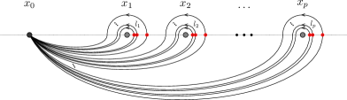
Figure 5.1. Illustration of the integration surface for a “basis integral function” $\varphi^{(x_{0})}_{l_{1},l_{2},\ldots,l_{p}}(x_{1},x_{2},\ldots,x_{p})$, that is, a Coulomb gas integral of type (5.3) with $\Gamma$ the surface depicted in the figure. The red circles indicate a choice of branch for the integrand in (5.3), so that it is real and positive when the integration variables lie at those points, see [KP20] for details. These integrals are the images under the spin chain – Coulomb gas correspondence map $\mathcal{F}$ of the natural basis vectors $e_{l_{p}}^{(d_{p})}\otimes\cdots\otimes e_{l_{2}}^{(d_{2})}\otimes e_{l_{1}}^{(d_{1})}$ of the tensor product representation (2.5), with $\ell=\sum_{i=1}^{p}l_{i}$.

5.2. The solutions with particular asymptotics

By Theorem 5.1, the projection properties (3.3) of the vectors $\mathfrak{v}_{\omega}$ of Theorem 3.1 give explicit asymptotic behavior for the solutions $\mathscr{F}_{\omega}=\mathcal{F}[\mathfrak{v}_{\omega}]$ when two variables $x_{j},x_{j+1}$ tend to a common limit. Furthermore, in Proposition 5.6 in the next section, we establish similar recursive asymptotics when taking many variables to a common limit.

Recall that, for a link pattern $\omega$, we denote by $\ell_{j,j+1}=\ell_{j,j+1}(\omega)$ the multiplicity of the link $\underset{\;\boldsymbol{j}\;\;\boldsymbol{j+1}}{\vbox{\hbox{\includegraphics[scale={0.5}]{link-0.pdf}}}}$ in $\omega$.

Theorem 5.3.

Let $\kappa\in(0,8)\setminus\mathbb{Q}$. The functions $\mathscr{F}_{\omega}=\mathcal{F}[\mathfrak{v}_{\omega}]\colon\mathfrak{X}_{p}\to\mathbb{C}$ have the following properties.

(1):

For any $\omega\in\mathrm{LP}_{\varsigma}^{(s)}$, the function $\mathscr{F}_{\omega}$ satisfies the Benoit $\&$ Saint-Aubin PDE system (PDE).

(2):

The function $\mathscr{F}_{\omega}$ is translation invariant and homogeneous as in (5.5), with $d=s+1$.

(3):

If $s=0$, then $\mathscr{F}_{\omega}$ satisfies the full Möbius covariance (5.6).

(4):

For any $j\in\{1,2,\ldots,p-1\}$ and $m=\frac{1}{2}\left(s_{j}+s_{j+1}-\delta+1\right)\in\{0,1,\ldots,\min(s_{j},s_{j+1})\}$, and $\xi\in(x_{j-1},x_{j+2})$, the function $\mathscr{F}_{\omega}$ has the asymptotics

(5.8) $$\lim_{x_{j},x_{j+1}\to\xi}\frac{\mathscr{F}_{\omega}(x_{1},\ldots,x_{p})}{|x_{j+1}-x_{j}|^{\Delta^{d_{j},d_{j+1}}_{\delta}}}=\; \begin{cases}0\quad&\mbox{if }\ell_{j,j+1}<m\\ \frac{B^{d_{j},d_{j+1}}_{\delta}}{\mathcal{C}({m;s_{j},s_{j+1}})}\times\mathscr{F}_{\hat{\omega}}(x_{1},\ldots,x_{j-1},\xi,x_{j+2}\ldots,x_{p})&\mbox{if }\ell_{j,j+1}=m,\\ \end{cases}$$

where $\hat{\omega}=\omega/(m\times\raisebox{2.15277pt}{ \scalebox{0.75}{$\underset{\;\boldsymbol{j}\;\;\boldsymbol{j+1}}{\vbox{\hbox{\includegraphics[scale={0.5}]{link-0.pdf}}}}$}})$, and the constants $B^{d_{j},d_{j+1}}_{\delta}$, given in Equation (5.7), and $\mathcal{C}({m;s_{j},s_{j+1}})$, given in Equation (3.10), are non-zero.

Proof.

Assertions (1) – (3) follow immediately from the properties (3.1) – (3.2) of the basis vectors $\mathfrak{v}_{\omega}$ of Theorem 3.1, and (PDE) and (COV) parts of Theorem 5.1. To prove assertion (4), we first note that, when $\kappa\in(0,8)$, then the exponents in the property (ASY) in Theorem 5.1 satisfy $\Delta_{\delta}^{d_{j},d_{j+1}}<\Delta_{\delta^{\prime}}^{d_{j},d_{j+1}}$, for any $2\leq\delta<\delta^{\prime}$, and for $\delta=1$ and $\delta^{\prime}\geq 3$, we also have $\Delta_{\delta^{\prime}}^{d_{j},d_{j+1}}-\Delta_{1}^{d_{j},d_{j+1}}>0$. Because in (5.8), $\delta$ increases in steps of two, we conclude that assertion (4) follows from the properties (3.3) of the basis vectors $\mathfrak{v}_{\omega}$ of Theorem 3.1 and the (ASY) part of Theorem 5.1. This concludes the proof. ∎

We remark that in the above theorem, the range of the parameter $\kappa$ is restricted to $(0,8)\setminus\mathbb{Q}$. The restriction to the interval $(0,8]$ is necessary in order to establish the asymptotics property (4). Indeed, when $\kappa>8$, the mutual order of the exponents in the formula (5.8) may change, resulting in the leading powers in the asymptotics to change. On the other hand, we expect the statement of Theorem 5.3 to be morally true also when $\kappa\in(0,8)\cap\mathbb{Q}$: functions $\mathscr{F}_{\omega}$ with properties (1) – (4) should still exist. In principle, the functions of Theorem 5.3 can be analytically continued to rational values of $\kappa$ — to do this systematically, further care would be needed.

Corollary 5.4.

The functions $\mathscr{F}_{\omega}$ are not identically zero.

Proof.

This follows from Theorem 5.3 by induction on the number $n=\sum_{i=1}^{p}s_{i}=:|\varsigma|$ for the link pattern $\omega\in\mathrm{LP}_{\varsigma}^{(s)}$ with $\varsigma=(s_{1},\ldots,s_{p})$. By Lemma 5.2, the base case is immediate, as $\mathscr{F}_{\emptyset}=\mathcal{F}[\mathfrak{v}_{\emptyset}]=\mathcal{F}[1]=1$. Fix $s\in\mathbb{Z}_{\geq 0}$ and assume that no function $\mathscr{F}_{\tau}$ with $\tau\in\mathrm{LP}_{\varrho}^{(s)}$ and $|\varrho|\leq n$ is identically zero. Consider a function $\mathscr{F}_{\omega}$ with $\omega\in\mathrm{LP}_{\varsigma}^{(s)}$, and $|\varsigma|=n+1$. First, if $\omega=\shuffle_{\lambda}$ only consists of defects, then the function $\mathscr{F}_{\omega}=\mathscr{F}_{\shuffle_{\lambda}}$ is not identically zero, by the explicit formula in Lemma 5.2. On the other hand, if $\omega$ contains links, then there is an innermost link $\raisebox{2.15277pt}{ \scalebox{0.75}{$\underset{\;\boldsymbol{j}\;\;\boldsymbol{j+1}}{\vbox{\hbox{\includegraphics[scale={0.5}]{link-0.pdf}}}}$}}\in\omega$. Applying the asymptotics property (5.8) with $m=\ell_{j,j+1}$, the induction hypothesis shows that $\mathscr{F}_{\omega}$ cannot be identically zero. ∎

5.3. Limits when collapsing several variables

      

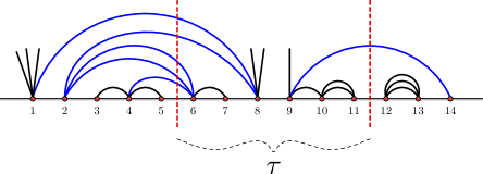
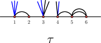
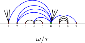
Figure 5.2. The sub-link pattern $\tau$ of a link pattern $\omega$, and the link pattern $\omega/\tau$, obtained from $\omega$ by removing the links of $\tau$ and collapsing the indices involved in $\tau$ into one point, colored in green. The lines which are colored in blue are common in both $\tau$ and $\omega/\tau$ — note that in $\tau$, these links are cut when separating $\tau$ from $\omega$ and they become defects, whereas $\omega/\tau$ has equally many defects as $\omega$, and the blue links remain.

We now consider the limit of the function $\mathscr{F}_{\omega}$ as several of its variables tend to a common limit simultaneously. For this, we need some notation.

Fix a link pattern

$$\omega=\Big{\{}\underset{\;a_{1}\;\;b_{1}}{\vbox{\hbox{\includegraphics[scale={0.5}]{link-0.pdf}}}},\ldots,\underset{\;a_{\ell}\;\;b_{\ell}}{\vbox{\hbox{\includegraphics[scale={0.5}]{link-0.pdf}}}}\Big{\}}\bigcup\Big{\{}\underset{c_{1}}{\vbox{\hbox{\includegraphics[scale={0.5}]{defect-0.pdf}}}},\ldots,\underset{c_{s}}{\vbox{\hbox{\includegraphics[scale={0.5}]{defect-0.pdf}}}}\Big{\}}\,\in\,\mathrm{LP}^{(s)}_{\varsigma}$$

and indices $1\leq j<k\leq p$, and denote by

$$\mathfrak{A}_{j,k}:=\; \left\{a_{i}\;|\;a_{i}\in\left\{j,j+1,\ldots,k\right\}\text{ and }\,b_{i}\notin\left\{j,j+1,\ldots,k\right\}\right\}\subset\left\{a_{1},a_{2},\ldots,a_{\ell}\right\},$$

$$\mathfrak{B}_{j,k}:=\; \left\{b_{i}\;|\;a_{i}\notin\left\{j,j+1,\ldots,k\right\}\text{ and }\,b_{i}\in\left\{j,j+1,\ldots,k\right\}\right\}\subset\left\{b_{1},b_{2},\ldots,b_{\ell}\right\},$$

$$\mathfrak{C}_{j,k}:=\; \left\{c_{i}\;|\;c_{i}\in\left\{j,j+1,\ldots,k\right\}\right\}\subset\left\{c_{1},c_{2},\ldots,c_{s}\right\},$$

and $r=\#\mathfrak{A}_{j,k}+\#\mathfrak{B}_{j,k}+\#\mathfrak{C}_{j,k}$, and let $\tau\in\mathrm{LP}_{\varsigma_{j,k}}^{(r)}$ be the sub-link pattern of $\omega$ with index valences $\varsigma_{j,k}=(s_{j},s_{j+1}\ldots,s_{k})$, consisting of the lines of $\omega$ attached to the indices $j,j+1,\ldots,k$, that is,

$$\tau=\tau_{j,k}(\omega)=\Big{\{}\underset{\;a_{i}\;\;b_{i}}{\vbox{\hbox{\includegraphics[scale={0.5}]{link-0.pdf}}}}\;\Big{|}\;a_{i},b_{i}\in\left\{j,j+1,\ldots,k\right\}\Big{\}}\bigcup\Big{\{}\underset{c}{\vbox{\hbox{\includegraphics[scale={0.5}]{defect-0.pdf}}}}\;\Big{|}\;c\in\mathfrak{A}_{j,k}\cup\mathfrak{B}_{j,k}\cup\mathfrak{C}_{j,k}\Big{\}}\,\in\,\mathrm{LP}_{\varsigma_{j,k}}^{(r)},$$

see Figure 5.2. Also, denote by $\omega/\tau$ the link pattern obtained from $\omega$ by “removing $\tau$”, that is, removing from $\omega$ the links $\underset{\;\boldsymbol{a\;}\;\;\boldsymbol{\;b\,}}{\vbox{\hbox{\includegraphics[scale={0.5}]{link-0.pdf}}}}$ with indices $a,b\in\{j,j+1,\ldots,k\}$, collapsing the indices $j,j+1,\ldots,k$ of $\omega$ into one point, and relabeling the indices thus obtained from left to right by $1,2,\ldots$, as emphasized in Figure 5.2.

The function $\mathscr{F}_{\omega}$ has the following limiting behavior.

Lemma 5.5.

Let $1\leq j<k\leq p$ and $x_{j-1}<\xi<x_{k+1}$, and suppose that

(5.9) $$\begin{split}&x_{j},x_{j+1},\ldots,x_{k}\to\xi\qquad\quad\text{ in such a way that }\qquad\frac{x_{i}-x_{j}}{x_{k}-x_{j}}\to\eta_{i},\qquad\text{ for }i\in\{j,j+1,\ldots,k\},\\ &\text{with }0=\eta_{j}<\eta_{j+1}<\cdots<\eta_{k-1}<\eta_{k}=1.\end{split}$$

Denote $\Delta=\Delta_{\delta}^{d_{j},\ldots,d_{k}}$, with $\delta=r+1$. Then, in the limit (5.9), we have

$$\frac{\mathscr{F}_{\omega}(x_{1},\ldots,x_{p})}{|x_{k}-x_{j}|^{\Delta}}\;\longrightarrow\;\; \mathscr{F}_{\tau}(\eta_{j},\ldots,\eta_{k})\times\mathscr{F}_{\omega/\tau}(x_{1},\ldots,x_{j-1},\xi,x_{k+1},\ldots,x_{p}).$$

Proof.

By Lemma C.3, for some constants $c_{l_{1},\ldots,l_{j-1};l;l_{k+1},\ldots,l_{p}}\in\mathbb{C}$, we have

(5.10) $$\mathfrak{v}_{\omega}=\; \sum_{l=0}^{r}\sum_{\begin{subarray}{c}l_{1},\ldots,l_{j-1},\\ l_{k+1},\ldots,l_{p}\end{subarray}}c_{l_{1},\ldots,l_{j-1};l;l_{k+1},\ldots,l_{p}}\times\left(e_{l_{p}}\otimes\cdots\otimes e_{l_{k+1}}\otimes F^{l}.\mathfrak{v}_{\tau}\otimes e_{l_{j-1}}\otimes\cdots\otimes e_{l_{1}}\right),$$

(5.11) $$\mathfrak{v}_{\omega/\tau}=\; \sum_{l=0}^{r}\sum_{\begin{subarray}{c}l_{1},\ldots,l_{j-1},\\ l_{k+1},\ldots,l_{p}\end{subarray}}c_{l_{1},\ldots,l_{j-1};l;l_{k+1},\ldots,l_{p}}\times\left(e_{l_{p}}\otimes\cdots\otimes e_{l_{k+1}}\otimes e_{l}\otimes e_{l_{j-1}}\otimes\cdots\otimes e_{l_{1}}\right).$$

Therefore, by [KP20, Proposition 5.1], the limit (5.9) has the asserted form:

$$\frac{\mathcal{F}[\mathfrak{v}_{\omega}](x_{1},\ldots,x_{p})}{|x_{k}-x_{j}|^{\Delta}}\;\longrightarrow\;\; \mathcal{F}[\mathfrak{v}_{\tau}](\eta_{j},\ldots,\eta_{k})\times\mathcal{F}[\mathfrak{v}_{\omega/\tau}](x_{1},\ldots,x_{j-1},\xi,x_{k+1},\ldots,x_{p}).$$

∎

In the proof of Lemma 5.5, we use [KP20, Proposition 5.1]. To prove the latter, the idea is to rearrange the integrations in the Coulomb gas type integral representation (5.3) of the function $\mathscr{F}_{\omega}=\mathcal{F}[\mathfrak{v}_{\omega}]$ in such a way that the collapsing variables $x_{j},\ldots,x_{k}$ are surrounded by nested contours — see Figure 5.3. After this rearranging, also “hypercube type” integrations between the variables $x_{j},\ldots,x_{k}$ might occur. Now, if the limit $x_{j},\ldots,x_{k}\to\xi$ is taken as in (5.9), then the function (5.3) with integration surface of Figure 5.3(top) converges to a function of type (5.3) with integration surface of Figure 5.3(bottom) times a constant which depends on the convergence rate (5.9). This multiplicative constant results in the constant $\mathscr{F}_{\tau}(\eta_{j},\ldots,\eta_{k})$ in Lemma 5.5. From its dependence on the convergence rate (5.9), we see that if the variables $x_{j},\ldots,x_{k}$ tend to $\xi$ in a different way, the limit can be different or fail to exist.

However, in some cases, no integrations between the collapsing variables $x_{j},\ldots,x_{k}$ occur, and then the limit Lemma 5.5 in fact exists along any sequence $x_{j},\ldots,x_{k}\to\xi$ and not only along sequences of type (5.9). Indeed, if in Figure 5.3 there are no contours between $x_{j},\ldots,x_{k}$, but only around them, then similarly as in the proof of [KP20, Proposition 5.1], dominated convergence theorem allows us to collapse these variables inside the integration in (5.3) along any sequence $x_{j},\ldots,x_{k}\to\xi$.

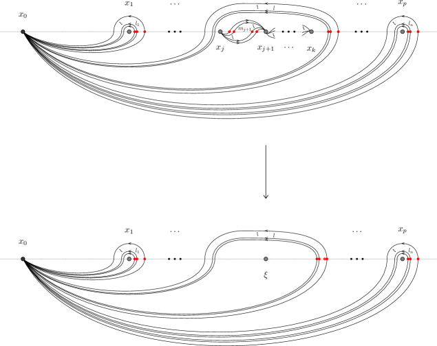
Figure 5.3. To deal with limits $x_{j},\ldots,x_{k}\to\xi$, the main idea is to write the integration surface $\Gamma$ of (5.3) as a linear combination of surfaces appearing in the top figure, where a number $l\geq 0$ of non-intersecting nested loops surround the collapsing points $x_{j},\ldots,x_{k}$ and there are $m_{j+1},\ldots,m_{k}\geq 0$ contours between these points. The latter form a “deformed hypercube integral” $\widetilde{\rho}_{0,m_{j+1},\ldots,m_{k}}(x_{j},\ldots,x_{k})$, illustrated in Figure 5.4, which can in some cases be evaluated explicitly. The red circles indicate a choice of branch for the integrand in (5.3), so that it is real and positive when the integration variables lie at those points, see [KP20] for details. The integral function (5.3) with surface $\Gamma$ as in the top figure is denoted by $\alpha^{(x_{0})}_{l_{1},\ldots l_{j-1};l,\{m_{j+1},\ldots,m_{k}\};l_{k+1},\ldots,l_{p}}(x_{1},\ldots,x_{p})$.

By changing the normalization of the function $\mathscr{F}_{\omega}$ in Lemma 5.5, we can remove the restriction (5.9).

Proposition 5.6.

Let $1\leq j<k\leq p$, and $x_{j-1}<\xi<x_{k+1}$. Then we have

(5.12) $$\lim_{x_{j},x_{j+1},\ldots,x_{k}\to\xi}\frac{\mathscr{F}_{\omega}(x_{1},\ldots,x_{p})}{\mathscr{F}_{\tau}(x_{j},\ldots,x_{k})}=\; \mathscr{F}_{\omega/\tau}(x_{1},\ldots,x_{j-1},\xi,x_{k+1},\ldots,x_{p}).$$

Proof.

First, by [KP20, Proposition 4.5], we can write $\mathscr{F}_{\tau}=\mathcal{F}[\mathfrak{v}_{\tau}]$ in the form

$$\mathcal{F}[\mathfrak{v}_{\tau}](x_{j},\ldots,x_{k})=\sum_{m_{j+1},\ldots,m_{k}\geq 0}a_{m_{j+1},\ldots,m_{k}}\times\widetilde{\rho}_{0,m_{j+1},\ldots,m_{k}}(x_{j},\ldots,x_{k}),$$

where $a_{m_{j+1},\ldots,m_{k}}\in\mathbb{C}$ are some constants, each $\widetilde{\rho}_{0,m_{j+1},\ldots,m_{k}}$ denotes a Coulomb gas integral of type (5.3) with $\Gamma$ a surface of type depicted in Figure 5.4, and

(5.13) $$m_{j+1}+\cdots+m_{k}=\frac{1}{2}\left(\sum_{i=j}^{k}d_{i}-k+j-\delta\right).$$

Second, by [KP20, Proof of Proposition 5.1], we can write the functions $\mathcal{F}^{(x_{0})}[v]$ for vectors

$$v=\left(e_{l_{p}}\otimes\cdots\otimes e_{l_{k+1}}\otimes F^{l}.\mathfrak{v}_{\tau}\otimes e_{l_{j-1}}\otimes\cdots\otimes e_{l_{1}}\right)$$

in the form

$$\mathcal{F}^{(x_{0})}[v](x_{1},\ldots,x_{p})=\sum_{m_{j+1},\ldots,m_{k}\geq 0}a_{m_{j+1},\ldots,m_{k}}\times\alpha^{(x_{0})}_{l_{1},\ldots,l_{j-1};l,\left\{m_{j+1},\ldots,m_{k}\right\};l_{k+1},\ldots,l_{p}}(x_{1},\ldots,x_{p}),$$

where each $\alpha^{(x_{0})}_{\cdots;l,\left\{m_{j+1},\ldots,m_{k}\right\};\cdots}$ denotes a Coulomb gas integral of type (5.3) with $\Gamma$ a surface of type depicted in Figure 5.3(top). We note that these integration surfaces a priori depend on an auxiliary point $x_{0}$, but as proved in [KP20, Proposition 4.5], all solutions to (PDE) are independent of $x_{0}$.

All in all, we can write the ratio appearing in the asserted equation (5.12) in the form

$$\frac{\mathcal{F}[\mathfrak{v}_{\omega}](x_{1},\ldots,x_{p})}{\mathcal{F}[\mathfrak{v}_{\tau}](x_{j},\ldots,x_{k})}$$

$$=\; \sum_{l=0}^{r}\sum_{\begin{subarray}{c}l_{1},\ldots,l_{j-1},\\ l_{k+1},\ldots,l_{p}\end{subarray}}c_{l_{1},\ldots,l_{j-1};l;l_{k+1},\ldots,l_{p}}\frac{\underset{m_{j+1},\ldots,m_{k}\geq 0}{\sum}a_{m_{j+1},\ldots,m_{k}}\times\alpha^{(x_{0})}_{l_{1},\ldots,l_{j-1};l,\left\{m_{j+1},\ldots,m_{k}\right\};l_{k+1},\ldots,l_{p}}(x_{1},\ldots,x_{p})}{\underset{m_{j+1},\ldots,m_{k}\geq 0}{\sum}a_{m_{j+1},\ldots,m_{k}}\times\widetilde{\rho}_{0,m_{j+1},\ldots,m_{k}}(x_{j},\ldots,x_{k})},$$

where we also used Equation (5.10).

Then, using Equation (5.11), we write the right hand side of the asserted equation (5.12) in the form

$$\mathcal{F}[\mathfrak{v}_{\omega/\tau}](x_{1},\ldots,x_{j-1},\xi,x_{k+1},\ldots,x_{p})$$

$$=\; \sum_{l=0}^{r}\sum_{\begin{subarray}{c}l_{1},\ldots,l_{j-1},\\ l_{k+1},\ldots,l_{p}\end{subarray}}c_{l_{1},\ldots,l_{j-1};l;l_{k+1},\ldots,l_{p}}\times\varphi^{(x_{0})}_{l_{1},\ldots,l_{j-1},l,l_{k+1},\ldots,l_{p}}(x_{1},\ldots,x_{j-1},\xi,x_{k+1},\ldots,x_{p}),$$

where each $\varphi^{(x_{0})}_{l_{1},\ldots,l_{j-1},l,l_{k+1},\ldots,l_{p}}$ denotes a Coulomb gas integral of type (5.3) with $\Gamma$ a surface of type depicted in Figure 5.1.

Now, to evaluate the limit (5.12), we can apply dominated convergence theorem to the integration over all variables in $\alpha^{(x_{0})}_{\cdots;l,\left\{m_{j+1},\ldots,m_{k}\right\};\cdots}$ whose contour is a loop, since these contours remain bounded away from the points $x_{j},\ldots,x_{k}$ and any hypercube type integration contours between them. On the other hand, we note that the hypercube integrals are the same in $\alpha^{(x_{0})}_{\cdots;l,\left\{m_{j+1},\ldots,m_{k}\right\};\cdots}$ and in $\widetilde{\rho}_{0,m_{j+1},\ldots,m_{k}}$, and they cancel each other in the limit (5.12). We also note that the remaining loop integrals in $\alpha^{(x_{0})}_{\cdots;l,\left\{m_{j+1},\ldots,m_{k}\right\};\cdots}$ are the same as in $\varphi^{(x_{0})}_{l_{1},\ldots,l_{j-1},l,l_{k+1},\ldots,l_{p}}$.

To finish, we consider the integrand (5.4) for $\alpha^{(x_{0})}_{\cdots;l,\left\{m_{j+1},\ldots,m_{k}\right\};\cdots}(x_{1},\ldots,x_{p})$:

$$\prod_{1\leq i<j\leq p}(x_{j}-x_{i})^{\frac{2}{\kappa}s_{i}s_{j}}\prod_{\begin{subarray}{c}1\leq i\leq p\\ 1\leq r\leq\ell\end{subarray}}(w_{r}-x_{i})^{-\frac{4}{\kappa}s_{i}}\prod_{1\leq r<s\leq\ell}(w_{s}-w_{r})^{\frac{8}{\kappa}}.$$

Using the identity (5.13), we see that as $x_{j},\ldots,x_{k}\to\xi$, the factors containing these variables converge to the corresponding factors in the integrand for $\varphi^{(x_{0})}_{l_{1},\ldots,l_{j-1},l,l_{k+1},\ldots,l_{p}}(x_{1},\ldots,x_{j-1},\xi,x_{k+1},\ldots,x_{p})$, where those terms have the form $(\xi-x_{i})^{\frac{2}{\kappa}s_{i}(\delta-1)}$ and $(w_{r}-\xi)^{-\frac{4}{\kappa}s_{i}(\delta-1)}$. This gives the asserted result. ∎

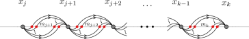
Figure 5.4. Illustration of the integration surface for a “deformed hypercube integral” $\widetilde{\rho}_{0,m_{j+1},\ldots,m_{k}}(x_{j},\ldots,x_{k})$. The red circles indicate a choice of branch for the integrand in (5.3), so that it is real and positive when the integration variables lie at those points, see [KP20] for details.

As a final remark, we observe that the functions $\mathscr{F}_{\omega}$ of Theorem 5.3 can be realized as limits of functions $\mathscr{F}_{\alpha(\omega)}=\mathcal{F}[v_{\alpha(\omega)}]$, where $\omega\mapsto\alpha(\omega)$ is the map (2.16) and $v_{\alpha}$ the vectors of Theorem 3.4. For the precise statement, we denote $n=|\varsigma|:=\sum_{i=1}^{p}s_{i}$, as in (2.13), and for $i\in\{1,\ldots,p\}$, we let $\lambda_{i}$ be the partition of $s_{i}$ into positive integers with size $|\lambda_{i}|=s_{i}$, that is, $\lambda_{i}=(1,1,\ldots,1)$ with $s_{i}$ parts all equal to one.

Corollary 5.7.

Along any sequence $(y_{1},\ldots,y_{n})\in\mathfrak{X}_{n}$ converging to $(x_{1},\ldots,x_{p})\in\mathfrak{X}_{p}$ as shown, we have

$$\mathscr{F}_{\omega}(x_{1},\ldots,x_{p})=\lim_{\begin{subarray}{c}\vspace*{1mm}\\ \hskip 18.49428pty_{1},\ldots,y_{s_{1}}\to x_{1}\\ \hskip 5.69054pty_{s_{1}+1},\ldots,y_{s_{2}}\to x_{2}\\ \vdots\\ y_{n-s_{p}+1},\ldots,y_{n}\to x_{p}\end{subarray}}\frac{\mathscr{F}_{\alpha(\omega)}(y_{1},\ldots,y_{n})}{\mathscr{F}_{\shuffle_{\lambda_{1}}}(y_{1},\ldots,y_{s_{1}})\mathscr{F}_{\shuffle_{\lambda_{2}}}(y_{s_{1}+1},\ldots,y_{s_{2}})\cdots\mathscr{F}_{\shuffle_{\lambda_{p}}}(y_{n-s_{p}+1},\ldots,y_{n})}.$$

Proof.

This follows from definitions and Proposition 5.6. The integral forms of the functions guarantee that we can take the limits in any order, and Proposition 5.6 that the limits exist along any sequence. ∎

The statement of Corollary 5.7 is very natural in the sense of fusion in CFT. Indeed, viewed as correlation functions, the solutions $\mathscr{F}_{\omega}$ should be obtained by fusion from the solutions $\mathscr{F}_{\alpha(\omega)}$. We also note that the functions $\mathscr{F}_{\shuffle_{\lambda_{i}}}$ appearing in the denominator in Corollary 5.7 have a simple form, given by Lemma 5.2.

5.4. Limits when taking variables to infinity

From the cyclic permutation symmetry of the vectors $\mathfrak{v}_{\omega}\in\mathsf{H}_{\varsigma}^{(0)}$ (Corollary 4.2) we can derive a similar property for the Möbius covariant functions $\mathscr{F}_{\omega}=\mathcal{F}[\mathfrak{v}_{\omega}]$, concerning the limit when the rightmost variable tends to $+\infty$. Indeed, this limit is equal to the limit of the function $\mathscr{F}_{\mathcal{S}(\omega)}$ as its leftmost variable tends to $-\infty$, where $\mathcal{S}$ is the cyclic permutation map defined in Equation (4.4) in Section 4, and illustrated in Figure 4.1.

Proposition 5.8.

For any $\omega\in\mathrm{LP}_{(\varsigma,s)}^{(0)}$, we have $($with $d=s+1)$

$$\lim_{y\to+\infty}\Big{(}y^{2h_{1,d}}\times\mathcal{F}[\mathfrak{v}_{\omega}](x_{1},\ldots,x_{p},y)\Big{)}=\lim_{y\to-\infty}\Big{(}|y|^{2h_{1,d}}\times\mathcal{F}[\mathfrak{v}_{\mathcal{S}(\omega)}](y,x_{1},\ldots,x_{p})\Big{)}.$$

Proof.

By [KP20, Proposition 5.4], we have

$$\lim_{y\to+\infty}\Big{(}y^{2h_{1,d}}\times\mathcal{F}[\mathfrak{v}_{\omega}](x_{1},\ldots,x_{p},y)\Big{)}= \;(q-q^{-1})^{d-1}\left[d-1\right]!^{2}\times B^{d,d}_{1}\times\mathcal{F}[R_{+}^{(s)}(\mathfrak{v}_{\omega})](x_{1},\ldots,x_{p}),$$

$$\lim_{y\to-\infty}\Big{(}|y|^{2h_{1,d}}\times\mathcal{F}[\mathfrak{v}_{\mathcal{S}(\omega)}](y,x_{1},\ldots,x_{p})\Big{)}= \;(q^{-2}-1)^{d-1}\left[d-1\right]!^{2}\times B^{d,d}_{1}\times\mathcal{F}[R_{-}^{(s)}(\mathfrak{v}_{\mathcal{S}(\omega)})](x_{1},\ldots,x_{p}),$$

where $B^{d,d}_{1}$ is the constant defined in (5.7). Using Corollary 4.2, we calculate

$$\lim_{y\to-\infty}\Big{(}|y|^{2h_{1,d}}\times\mathcal{F}[\mathfrak{v}_{\mathcal{S}(\omega)}](y,x_{1},\ldots,x_{p})\Big{)}$$

$$= \;\frac{(q^{-2}-1)^{d-1}\left[d-1\right]!^{2}\times B^{d,d}_{1}\times(-q)^{d-1}}{(q-q^{-1})^{d-1}\left[d-1\right]!^{2}\times B^{d,d}_{1}}\lim_{y\to+\infty}\Big{(}y^{2h_{1,d}}\times\mathcal{F}[\mathfrak{v}_{\omega}](x_{1},\ldots,x_{p},y)\Big{)}$$

$$= \;\lim_{y\to+\infty}\Big{(}y^{2h_{1,d}}\times\mathcal{F}[\mathfrak{v}_{\omega}](x_{1},\ldots,x_{p},y)\Big{)}.$$

∎

6. Cyclic permutation symmetry of the pure partition functions of multiple $\mathrm{SLE}$s

Multiple $(\mathrm{SLE}_{\kappa})_{\kappa\geq 0}$ is a collection of random conformally invariant curves started from given boundary points of a simply connected domain, and connecting them pairwise without crossing [BBK05, Dub07, KL07, KP16, PW19]. Such curves describe scaling limits of interfaces in statistical mechanics models. Indeed, convergence of a single interface to the $\mathrm{SLE}_{\kappa}$ has now been proven for a number of models, see, e.g., [Smi01, LSW04, SS05, Smi06, Zha08, HK13, CDCH⁺14], and convergence of several interfaces to multiple $\mathrm{SLE}$s has also been established in some cases [CN06, Izy17, BPW18, KS18].

A multiple $\mathrm{SLE}$ can be constructed as a growth process encoded in a Loewner chain, see [Sch00, Dub07, KP16, PW19]. As an input for the construction, one uses a function $\mathcal{Z}\colon\mathfrak{X}_{2N}\to\mathbb{R}_{>0}$, called a partition function of the multiple $\mathrm{SLE}_{\kappa}$. This function appears in the Radon-Nikodym derivative of the multiple $\mathrm{SLE}_{\kappa}$ measure with respect to the product measure of independent $\mathrm{SLE}_{\kappa}$ curves. It must satisfy the second order PDE system

(6.1) $$\left[\frac{\kappa}{2}\frac{\partial^{2}}{\partial x_{i}^{2}}+\sum_{j\neq i}\left(\frac{2}{x_{j}-x_{i}}\frac{\partial}{\partial x_{j}}-\frac{2h_{1,2}}{(x_{j}-x_{i})^{2}}\right)\right]\mathcal{Z}(x_{1},\ldots,x_{2N})=0,\qquad\text{for all }i\in\{1,2,\ldots,2N\}.$$

With translation invariance, (6.1) are equivalent to the second order Benoit & Saint-Aubin PDEs. Furthermore, by conformal invariance of the multiple $\mathrm{SLE}_{\kappa}$, the partition function $\mathcal{Z}$ must be covariant under all Möbius transformations $\mu\colon\mathbb{H}\to\mathbb{H}$ such that $\mu(x_{1})<\mu(x_{2})<\cdots<\mu(x_{p})$:

$$\mathcal{Z}(x_{1},\ldots,x_{2N})=\prod_{i=1}^{2N}\mu^{\prime}(x_{i})^{h_{1,2}}\times\mathcal{Z}\left(\mu(x_{1}),\ldots,\mu(x_{2N})\right).$$

The law of the multiple $\mathrm{SLE}_{\kappa}$ is not unique, for the random curves may have several topological connectivities of the marked boundary points. The connectivities are encoded in planar pair partitions $\alpha\in\mathrm{PP}_{N}$. In fact, the convex set of probability measures of (local) multiple $\mathrm{SLE}_{\kappa}$ processes is in one-to-one correspondence with the set of positive (and normalized) partition functions $\mathcal{Z}$ — see [Dub07, KP16]. The extremal points of this convex set correspond to the different possible connectivities [PW19].

Pertaining to the construction of the extremal processes, in [KP16] a basis $\left(\mathcal{Z}_{\alpha}\right)_{\alpha\in\mathrm{PP}_{N}}$ of Möbius covariant solutions to the PDE system (6.1) was constructed, using Theorem 5.1 and the vectors $v_{\alpha}$ of Theorem 3.4. A defining property of the basis functions $\mathcal{Z}_{\alpha}$ is the recursive asymptotics property

(6.2) $$\lim_{x_{j},x_{j+1}\to\xi}\frac{\mathcal{Z}_{\alpha}(x_{1},\ldots,x_{2N})}{|x_{j+1}-x_{j}|^{-2h_{1,2}}}=\; \begin{cases}0\quad&\text{if }\underset{\;j\;\;j+1}{\vbox{\hbox{\includegraphics[scale={0.5}]{link-0.pdf}}}}\notin\alpha\\ \mathcal{Z}_{\hat{\alpha}}(x_{1},\ldots,x_{j-1},x_{j+2},\ldots,x_{2N})&\text{if }\underset{\;j\;\;j+1}{\vbox{\hbox{\includegraphics[scale={0.5}]{link-0.pdf}}}}\in\alpha,\end{cases}$$

with $\hat{\alpha}=\alpha/\raisebox{2.15277pt}{ \scalebox{0.75}{$\underset{\;\boldsymbol{j}\;\;\boldsymbol{j+1}}{\vbox{\hbox{\includegraphics[scale={0.5}]{link-0.pdf}}}}$}}$, for any $x_{j-1}<\xi<x_{j+2}$ and $j\in\{1,2,\ldots,2N-1\}$, and $\kappa\in(0,8)\setminus\mathbb{Q}$.

In [KP16], these functions $\mathcal{Z}_{\alpha}$ were called the pure partition functions of the multiple $\mathrm{SLE}_{\kappa}$. They were argued to be the partition functions of the extremal multiple $\mathrm{SLE}_{\kappa}$ processes, with the deterministic connectivities $\alpha$. A proof for this fact appeared recently in [PW19] in the case $0<\kappa\leq 4$.

Specifically, with $q=e^{\mathfrak{i}\pi 4/\kappa}$, the pure partition functions were constructed in [KP16] as

$$\mathcal{Z}_{\alpha}:=(B^{2,2}_{1})^{-N}\mathcal{F}[v_{\alpha}],\qquad\text{for }\alpha\in\mathrm{PP}_{N},$$

with the normalization constant chosen in such a way that the functions $\mathcal{Z}_{\alpha}$ satisfy the asymptotics (6.2) with no constants in front. The property (6.2) is in fact a special case of Theorem 5.3, and indeed, the more general functions $\mathscr{F}_{\omega}=\mathcal{F}[\mathfrak{v}_{\omega}]$ should provide pure partition functions of systems of multiple $\mathrm{SLE}_{\kappa}$ curves growing from the boundary, in the spirit of [FW03, Kon03, FK04, Dup06, KS07, Dub15b]. Also, the functions $\mathscr{F}_{\omega}$ describe observables concerning geometric properties of interfaces — see, e.g., [GC05, BJV13, Dub15b, JJK16, KKP20, LV19a, LV19b, PW19].

In Corollary 6.2 we show that the property (6.2) of the pure partition functions $\mathcal{Z}_{\alpha}$ is also true when taking the limit $x_{1}\to-\infty$ and $x_{2N}\to+\infty$, corresponding to the removal of the link $\underset{\;\boldsymbol{1}\;\;\boldsymbol{2N}}{\vbox{\hbox{\includegraphics[scale={0.5}]{link-0.pdf}}}}$ . We also consider the more general pure partition functions

(6.3) $$\mathcal{Z}_{\alpha}:=(B_{1}^{2,2})^{-N}\mathscr{F}_{\alpha},\qquad\text{for }\alpha\in\mathrm{PP}_{N}^{(s)},$$

which are homogeneous solutions to the second order PDEs (6.1), but, when $s>0$, not covariant under all Möbius maps in the covariance formula (5.6). We prove in Proposition 6.3 that these functions are linearly independent, and thus obtain a basis of a solution space of the PDE system (6.1).

6.1. Cyclic permutation symmetry

Corollary 4.2 gives a general cyclic permutation symmetry of the vectors $\mathfrak{v}_{\omega}\in\mathsf{H}_{\varsigma}^{(0)}\subset\bigotimes_{i=1}^{p}\mathsf{M}_{d_{i}}$ in the trivial subrepresentation. The special case of $n=2N$, with $d_{i}=2$, for all $i$, can be used in applications to the properties of the pure partition functions $\mathcal{Z}_{\alpha}$.

First, from Proposition 5.8 we immediately get the following corollary.

Corollary 6.1.

Let $\kappa\in(0,\infty)\setminus\mathbb{Q}$. Then we have

$$\lim_{y\to+\infty}\Big{(}y^{2h_{1,2}}\times\mathcal{Z}_{\alpha}(x_{1},\ldots,x_{2N-1},y)\Big{)}=\lim_{y\to-\infty}\Big{(}|y|^{2h_{1,2}}\times\mathcal{Z}_{\mathcal{S}(\alpha)}(y,x_{1},\ldots,x_{2N-1})\Big{)}.$$

Proof.

The assertion follows directly from the definition $\mathcal{Z}_{\alpha}:=(B_{1}^{2,2})^{-N}\mathcal{F}[v_{\alpha}]$ and Proposition 5.8. ∎

Using this, we can extend the cascade property (6.2) for the pure partition functions to $j=2N$.

Corollary 6.2.

Let $\kappa\in(0,8)\setminus\mathbb{Q}$. Denote by $\hat{\alpha}=\alpha/\raisebox{2.15277pt}{ \scalebox{0.75}{$\underset{\;\boldsymbol{1}\;\;\boldsymbol{2N}}{\vbox{\hbox{\includegraphics[scale={0.5}]{link-0.pdf}}}}$}}$. Then we have

$$\lim_{\begin{subarray}{c}x_{1}\to-\infty,\\ x_{2N}\to+\infty\end{subarray}}|x_{2N}-x_{1}|^{2h_{1,2}}\times\mathcal{Z}_{\alpha}(x_{1},\ldots,x_{2N})=\; \begin{cases}0\quad&\text{if }\underset{\;1\;\;2N}{\vbox{\hbox{\includegraphics[scale={0.5}]{link-0.pdf}}}}\notin\alpha\\ \mathcal{Z}_{\hat{\alpha}}(x_{2},\ldots,x_{2N-1})&\text{if }\underset{\;1\;\;2N}{\vbox{\hbox{\includegraphics[scale={0.5}]{link-0.pdf}}}}\in\alpha.\end{cases}$$

Proof.

We can take either limit first and get the same result. Observe first that we have $\raisebox{2.15277pt}{ \scalebox{0.75}{$\underset{\;\boldsymbol{1}\;\;\boldsymbol{2N}}{\vbox{\hbox{\includegraphics[scale={0.5}]{link-0.pdf}}}}$}}\in\alpha$ if and only if $\raisebox{2.15277pt}{ \scalebox{0.75}{$\underset{\;\boldsymbol{1\;}\;\;\boldsymbol{\;2\;}}{\vbox{\hbox{\includegraphics[scale={0.5}]{link-0.pdf}}}}$}}\in\mathcal{S}(\alpha)$, and in that case, $\mathcal{S}(\alpha)/\raisebox{2.15277pt}{ \scalebox{0.75}{$\underset{\;\boldsymbol{1\;}\;\;\boldsymbol{\;2\;}}{\vbox{\hbox{\includegraphics[scale={0.5}]{link-0.pdf}}}}$}}=\alpha/\raisebox{2.15277pt}{ \scalebox{0.75}{$\underset{\;\boldsymbol{1}\;\;\boldsymbol{2N}}{\vbox{\hbox{\includegraphics[scale={0.5}]{link-0.pdf}}}}$}}$. Using Corollary 6.1, the asymptotics property (6.2) for $\mathcal{Z}_{\mathcal{S}(\alpha)}$, and the above observation concerning the links, we can calculate the limit

$$\lim_{x_{1}\to-\infty}\lim_{x_{2N}\to+\infty}|x_{2N}-x_{1}|^{2h_{1,2}}\times\mathcal{Z}_{\alpha}(x_{1},\ldots,x_{2N})$$

$$= \;\lim_{x_{1}\to-\infty}\lim_{x_{2N}\to-\infty}|x_{2N}-x_{1}|^{2h_{1,2}}\times\mathcal{Z}_{\mathcal{S}(\alpha)}(x_{2N},x_{1},x_{2}\ldots,x_{2N-1})$$

$$= \;\begin{cases}0\quad&\text{if }\underset{\;1\;\;\;\;2\;}{\vbox{\hbox{\includegraphics[scale={0.5}]{link-0.pdf}}}}\notin\mathcal{S}(\alpha)\\ \mathcal{Z}_{\mathcal{S}(\alpha)/\underset{\scriptscriptstyle{\,1\;\,\;2\;}}{\vbox{\hbox{\includegraphics[scale={0.2}]{link-0.pdf}}}}}(x_{2},\ldots,x_{2N-1})&\text{if }\underset{\;1\;\;\;\;2\;}{\vbox{\hbox{\includegraphics[scale={0.5}]{link-0.pdf}}}}\in\mathcal{S}(\alpha)\end{cases}$$

$$= \;\begin{cases}0\quad&\text{if }\underset{\;1\,\;\;\,2N}{\vbox{\hbox{\includegraphics[scale={0.5}]{link-0.pdf}}}}\notin\alpha\\ \mathcal{Z}_{\alpha/\underset{\scriptscriptstyle{\,1\,\,\,2N}}{\vbox{\hbox{\includegraphics[scale={0.2}]{link-0.pdf}}}}}(x_{2},\ldots,x_{2N-1})&\text{if }\underset{\;1\,\;\;\,2N}{\vbox{\hbox{\includegraphics[scale={0.5}]{link-0.pdf}}}}\in\alpha.\end{cases}$$

∎

Corollary 6.2 combined with Equation (6.2) shows that linear combinations of the basis functions $\mathcal{Z}_{\alpha}$ have a cascade property with respect to removing any link connecting consecutive points, when the boundary $\partial\mathbb{H}=\mathbb{R}$ is viewed as the circle $\mathbb{S}^{1}=\left\{z\in\mathbb{C}\;\big{|}\;|z=1|\right\}$, say. Such a property is natural for the random $\mathrm{SLE}_{\kappa}$ type curves — see Figure 6.1 for an illustration. In fact, this cascade property can be taken as a defining property of a global multiple $\mathrm{SLE}_{\kappa}$, see [KL07, PW19].

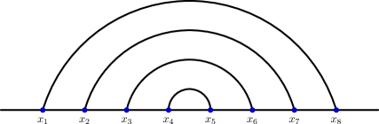
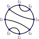
Figure 6.1. The probability measure of multiple $\mathrm{SLE}_{\kappa}$ curves is conformally invariant. The figure depicts how a connectivity of the curves is mapped under a conformal map from the upper half-plane $\mathbb{H}$ to the disc $\mathbb{D}$. The starting points $x_{1}<x_{2}<\ldots<x_{2N}$ of the curves in $\mathbb{H}$ are mapped to the points $\xi_{1},\xi_{2},\ldots,\xi_{2N}$ appearing in counterclockwise order along the boundary of $\mathbb{D}$. The cascade property (6.2) given in Corollary 6.2 for the outermost link connecting $x_{1}$ and $x_{2N}$ is manifest in the disc on the right.

6.2. Linear independence for solutions to second order PDEs

We now consider the functions $\mathcal{Z}_{\alpha}$, with $\alpha\in\mathrm{PP}_{N}^{(s)}$, defined in Equation (6.3). These functions form a basis of the solution space of the second order PDE system (6.1), consisting of homogeneous solutions, in the sense of items (1) and (2) in Theorem 5.3. With $n=2N+s$, this solution space is the image $\mathcal{F}[\mathsf{H}_{n}^{(s)}]$ of the highest weight vector space $\mathsf{H}_{n}^{(s)}$ under the map $\mathcal{F}$ of Theorem 5.1. We prove the linear independence of the functions $\mathcal{Z}_{\alpha}$ by constructing a basis for the dual space

$$\mathcal{F}[\mathsf{H}_{n}^{(s)}]^{*}=\left\{\psi\colon\mathsf{H}_{n}^{(s)}\to\mathbb{C}\;|\;\psi\text{ is a linear map}\right\},$$

using similar ideas as in [KP16, Section 4.2], where the case $s=0$ was treated.

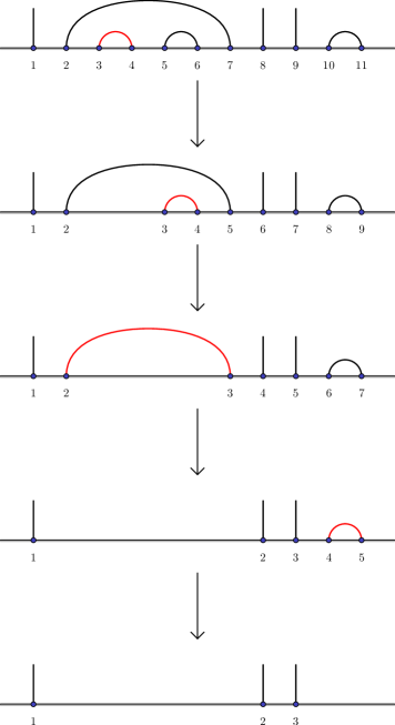
Figure 6.2. Example of an allowable ordering to remove links. After the removal of all the links, the defects remain. Notice also the relabeling of the indices after each step

Proposition 6.3.

Let $\kappa\in(0,8)\setminus\mathbb{Q}$, $s\in\mathbb{Z}_{\geq 0}$, and $n=2N+s\in\mathbb{Z}_{>0}$. The collection $\left(\mathcal{Z}_{\alpha}\right)_{\alpha\in\mathrm{PP}_{N}^{(s)}}$ is a basis of the solution space $\mathcal{F}[\mathsf{H}_{n}^{(s)}]$ of dimension $\frac{s+1}{N+s+1}\binom{2N+s}{N+s}$.

Proof.

The case $s=0$ was proved in [KP16, Proposition 4.2]. The case $s>0$ is very similar, so we only give the idea of the proof. We consider the links in the link pattern

$$\alpha=\Big{\{}\underset{\;a_{1}\;\;b_{1}}{\vbox{\hbox{\includegraphics[scale={0.5}]{link-0.pdf}}}},\ldots,\underset{\;a_{N}\;\;b_{N}}{\vbox{\hbox{\includegraphics[scale={0.5}]{link-0.pdf}}}}\Big{\}}\bigcup\Big{\{}\underset{c_{1}}{\vbox{\hbox{\includegraphics[scale={0.5}]{defect-0.pdf}}}},\ldots,\underset{c_{s}}{\vbox{\hbox{\includegraphics[scale={0.5}]{defect-0.pdf}}}}\Big{\}}\,\in\,\mathrm{PP}_{N}^{(s)}$$

as an ordered set, see Appendix C and [KP16, Section 3.5] for details. We say that the ordering of the links is allowable for $\alpha$ if all links of $\alpha$ can be removed in such a way that at each step, the link to be removed connects two consecutive indices — see Figure 6.2 for an illustration. The precise definition of “allowability” was given in [KP16, Section 3.5] for the case $s=0$, but as the defects of $\alpha$ play no role in the link removal and no defects lie inside any link, the notion of an allowable ordering of links is the same for any $\alpha\in\mathrm{PP}_{N}^{(s)}$.

Suppose that the ordering of the links in $\alpha$ is allowable. Then, by Theorem 5.3, the iterated limit

$$\mathscr{L}_{\alpha}(\mathcal{F}[v]):=\; \lim_{x_{a_{N}},x_{b_{N}}\to\xi_{N}}\cdots\lim_{x_{a_{1}},x_{b_{1}}\to\xi_{1}}(x_{b_{N}}-x_{a_{N}})^{2h_{1,2}}\cdots(x_{b_{1}}-x_{a_{1}})^{2h_{1,2}}\times\mathcal{F}[v](x_{1},\ldots,x_{n})$$

exists for any $v\in\mathsf{H}_{n}^{(s)}$. Consider the image $\mathscr{F}_{\alpha}=\mathcal{F}[\mathfrak{v}_{\alpha}]$ of the basis vector $\mathfrak{v}_{\alpha}\in\mathsf{H}_{n}^{(s)}$. Suppose that $c_{1}<c_{2}<\cdots<c_{s}$, and denote by $y_{i}=x_{c_{i}}$, for $i\in\{1,2,\ldots,s\}$. Using the property (5.8) of $\mathscr{F}_{\alpha}$ with the constant $\mathcal{C}({1;1,1})=1$ given by Equation (3.10), we evaluate the limit $\mathscr{L}_{\alpha}(\mathscr{F}_{\alpha})$ as

$$\mathscr{L}_{\alpha}(\mathscr{F}_{\alpha})(y_{1},\ldots,y_{s})=(B_{1}^{2,2})^{N}\times\mathscr{F}_{\shuffle_{\lambda}}(y_{1},\ldots,y_{s}),\qquad\text{for }\alpha\in\mathrm{PP}_{N}^{(s)},$$

where $\lambda=(1,1,\ldots,1,1)\in\mathbb{Z}^{s}$ and $\mathscr{F}_{\shuffle_{\lambda}}$ has the explicit formula given in Lemma 5.2. With the identification $\mathfrak{v}_{\shuffle_{\lambda}}\mapsto 1$ as in Remark 3.2, and the formula in Lemma 5.2, we may interpret $\mathscr{L}_{\alpha}(\mathcal{Z}_{\alpha})=1$.

On the other hand, if $\beta\neq\alpha$, then the limit $\mathscr{L}_{\alpha}(\mathscr{F}_{\beta})$ evaluates to zero, because of the property (5.8) and the fact that when $\beta\neq\alpha$, then we have $\raisebox{2.15277pt}{ \scalebox{0.75}{$\underset{\;\boldsymbol{a_{j}}\;\;\boldsymbol{b_{j}}}{\vbox{\hbox{\includegraphics[scale={0.5}]{link-0.pdf}}}}$}}\notin\beta$, for some link $\raisebox{2.15277pt}{ \scalebox{0.75}{$\underset{\;\boldsymbol{a_{j}}\;\;\boldsymbol{b_{j}}}{\vbox{\hbox{\includegraphics[scale={0.5}]{link-0.pdf}}}}$}}\in\alpha$ in the allowable ordering.

It follows that the map $\mathscr{L}_{\alpha}\colon\mathcal{F}[\mathsf{H}_{n}^{(s)}]\rightarrow\mathbb{C}$ is well-defined and independent of the choice of the allowable ordering for $\alpha$. In particular, the collection $\left(\mathscr{L}_{\alpha}\right)_{\alpha\in\mathrm{PP}_{N}^{(s)}}$ is a basis of the dual space $\mathcal{F}[\mathsf{H}_{n}^{(s)}]^{*}$, such that

$$\mathscr{L}_{\alpha}(\mathcal{Z}_{\beta})=\delta_{\alpha,\beta}=\; \begin{cases}1\quad&\text{if }\beta=\alpha\\ 0&\text{if }\beta\neq\alpha.\end{cases}$$

Therefore, $\left(\mathcal{Z}_{\alpha}\right)_{\alpha\in\mathrm{PP}_{N}^{(s)}}$ is a basis of the solution space $\mathcal{F}[\mathsf{H}_{n}^{(s)}]$, dual to $\left(\mathscr{L}_{\alpha}\right)_{\alpha\in\mathrm{PP}_{N}^{(s)}}$. The formula for the dimension of this space follows from Lemma 2.2 and [KP16, Lemma 2.2]: $\#\mathrm{PP}_{N}^{(s)}=\frac{s+1}{N+s+1}\binom{2N+s}{N+s}$. ∎

The linear independence of the functions $\mathcal{Z}_{\alpha}$ immediately gives injectivity of the “spin chain – Coulomb gas correspondence” map $\mathcal{F}$ in the case of $\varsigma=(1,1,\ldots,1,1)$ and $s\geq 0$. This generalizes the previous injectivity result [KP16, Corollary 4.3]. We prove the injectivity of $\mathcal{F}$ in full generality in forthcoming work [FP20b⁺], where we study solution spaces of the Benoit & Saint-Aubin PDEs in detail.

Corollary 6.4.

For $s\in\mathbb{Z}_{\geq 0}$ and $n=2N+s\in\mathbb{Z}_{>0}$, the map $\mathcal{F}\colon\mathsf{H}_{n}^{(s)}\rightarrow\mathcal{C}^{\infty}(\mathfrak{X}_{n})$ is injective.

Proof.

The assertion follows by linearity from Propositions 3.7 and 6.3 — the images $\mathscr{F}_{\alpha}=\mathcal{F}[\mathfrak{v}_{\alpha}]$ of the basis vectors $\mathfrak{v}_{\alpha}$ of $\mathsf{H}_{n}^{(s)}$ are linearly independent, because the functions $\mathcal{Z}_{\alpha}=(B_{1}^{2,2})^{-N}\mathcal{F}[\mathfrak{v}_{\alpha}]$ are. ∎

Appendix A $q$-combinatorics

In this appendix, we prove “$q$-combinatorial formulas” needed in this article. We first recall the definitions

$$\left[m\right]=\; \frac{q^{m}-q^{-m}}{q-q^{-1}},\qquad\qquad\left[n\right]!=\prod_{m=1}^{n}\left[m\right],\qquad\qquad\left[\begin{array}[]{c}n\\ k\end{array}\right]=\frac{\left[n\right]!}{\left[k\right]!\left[n-k\right]!},$$

for $q\in\mathbb{C}\setminus\left\{0\right\}$ not a root of unity, and $m\in\mathbb{Z}$, and $n,k\in\mathbb{N}$, with $0\leq k\leq n$.

Lemma A.1.

(a):

The $q$-binomial coefficients satisfy the recursion

$$\left[\begin{array}[]{c}n\\ k\end{array}\right]=q^{k}\left[\begin{array}[]{c}n-1\\ k\end{array}\right]+q^{k-n}\left[\begin{array}[]{c}n-1\\ k-1\end{array}\right].$$

(b):

[KP20, Lemma 2.1(b)] For a permutation $\sigma\in\mathfrak{S}_{n}$ of $\left\{1,2,\ldots,n\right\}$, denote by

$${\rm inv}(\sigma)=\; \left\{(i,j)\;\big{|}\;i<j\text{ and }\sigma(i)>\sigma(j)\right\}$$

the set of inversions of $\sigma$. Then we have

$$\sum_{\sigma\in\mathfrak{S}_{n}}q^{2\times\#{\rm inv}(\sigma)}=\; q^{{\binom{n}{2}}}\left[n\right]!.$$

(c):

For any $\nu_{1},\nu_{2}\in\mathbb{Z}_{\geq 0}$ and $n\in\mathbb{N}$, we have

$$\sum_{k=0}^{n}\left[\begin{array}[]{c}n\\ k\end{array}\right]q^{k(2n-\nu_{1}-\nu_{2}-2)}\left[\nu_{1}-n+k\right]!\left[\nu_{2}-k\right]!\;=\;\; q^{n(n-\nu_{1}-1)}\frac{\left[\nu_{1}-n\right]!\left[\nu_{2}-n\right]!\left[\nu_{1}+\nu_{2}-n+1\right]!}{\left[\nu_{1}+\nu_{2}-2n+1\right]!}.$$

(d):

For any $\nu_{1},\nu_{2}\in\mathbb{Z}_{\geq 0}$ and $n\in\mathbb{N}$, we have

$$\sum_{k=0}^{n}\left[\begin{array}[]{c}n\\ k\end{array}\right]q^{k(\nu_{1}+\nu_{2}-2n+2)}\left[\nu_{1}-k\right]!\left[\nu_{2}-n+k\right]!\;=\;\; q^{n(\nu_{2}+1-n)}\frac{\left[\nu_{1}-n\right]!\left[\nu_{2}-n\right]!\left[\nu_{1}+\nu_{2}-n+1\right]!}{\left[\nu_{1}+\nu_{2}-2n+1\right]!}.$$

Proof.

The proof of (a) is a straightforward calculation using the definition of $q$-integers. Part (b) was proved in [KP20, Lemma 2.1(b)]. To prove part (c), we proceed by induction on $n$. For $n=0$, both sides of the equation are equal to $\left[\nu_{1}\right]!\left[\nu_{2}\right]!$. Denote by $L_{n}(\nu_{1},\nu_{2})$ and $R_{n}(\nu_{1},\nu_{2})$ the left and right hand sides of the asserted equation, respectively, and assume that we have $L_{n}(\nu_{1},\nu_{2})=R_{n}(\nu_{1},\nu_{2})$, for any $\nu_{1},\nu_{2}\in\mathbb{Z}_{\geq 0}$. Using part (a), we write $L_{n+1}(\nu_{1},\nu_{2})$ as

$$L_{n+1}(\nu_{1},\nu_{2})=\; \sum_{k=0}^{n}\left[\begin{array}[]{c}n\\ k\end{array}\right]q^{k(2n+1-\nu_{1}-\nu_{2})}\left[\nu_{1}-n+k\right]!\left[\nu_{2}-k\right]!\left(\frac{1}{\left[\nu_{1}-n+k\right]}+q^{n-\nu_{1}-\nu_{2}}\frac{1}{\left[\nu_{2}-k\right]}\right)$$

$$=\; \sum_{k=0}^{n}\left[\begin{array}[]{c}n\\ k\end{array}\right]q^{k(2n-\nu_{1}-\nu_{2})}\left[\nu_{1}-n+k\right]!\left[\nu_{2}-k\right]!\,q^{n-\nu_{1}}\frac{\left[\nu_{1}+\nu_{2}-n\right]}{\left[\nu_{2}-k\right]\left[\nu_{1}-n+k\right]}$$

$$=\; \left[\nu_{1}+\nu_{2}-n\right]q^{n-\nu_{1}}\times\sum_{k=0}^{n}\left[\begin{array}[]{c}n\\ k\end{array}\right]q^{k(2n-\nu_{1}-\nu_{2})}\left[\nu_{1}-1-n+k\right]!\left[\nu_{2}-1-k\right]!,$$

where we used the identity

$$q^{n-k-\nu_{1}}\left[\nu_{1}+\nu_{2}-n\right]=\left[\nu_{2}-k\right]+q^{n-\nu_{1}-\nu_{2}}\left[\nu_{1}-n+k\right].$$

By the induction hypothesis, the above sum is equal to $L_{n}(\nu_{1}-1,\nu_{2}-1)=R_{n}(\nu_{1}-1,\nu_{2}-1)$, so

$$L_{n+1}(\nu_{1},\nu_{2})=\; \left[\nu_{1}+\nu_{2}-n\right]q^{n-\nu_{1}}\times R_{n}(\nu_{1}-1,\nu_{2}-1)$$

$$=\; \left[\nu_{1}+\nu_{2}-n\right]q^{n-\nu_{1}}\times q^{n(n-\nu_{1})}\frac{\left[\nu_{1}-1-n\right]!\left[\nu_{2}-1-n\right]!\left[\nu_{1}+\nu_{2}-n-1\right]!}{\left[\nu_{1}+\nu_{2}-2n-1\right]!}$$

$$=\; R_{n+1}(\nu_{1},\nu_{2}),$$

as claimed. This concludes the proof of (c).

Assertion (d) follows immediately from (c) and the symmetries $q\leftrightarrow q^{-1}$ and $\nu_{1}\leftrightarrow\nu_{2}$ of the identity. ∎

Appendix B Some auxiliary calculations

In this appendix, we perform some auxiliary calculations needed in the proof of Lemma 3.10 and Proposition 3.11. We will repeatedly use the notations (2.7),

$$s=d-1,\qquad s_{i}=d_{i}-1,\quad\text{ for all }i\in\{1,2,\ldots,p\},\qquad\text{ and }\qquad\varsigma=(s_{1},s_{2},\ldots,s_{p})\in\mathbb{Z}_{\geq 0}^{p}.$$

In the calculations, we consider the embedding from Section 3.1, defined for any $s=d-1\in\mathbb{Z}_{>0}$ as

$$\mathfrak{I}^{(s)}\colon\mathsf{M}_{d}\hookrightarrow\mathsf{M}_{2}^{\otimes s},\qquad\mathfrak{I}^{(s)}(e_{l}^{(d)}):=\theta_{l}^{(s)},\quad\text{ for }l\in\{0,1,\ldots,s\}.$$

The vectors $\theta_{l}^{(s)}$ can be written explicitly as follows.

Lemma B.1.

In the tensor product $\mathsf{M}_{2}^{\otimes s}$, we have

$$\mathfrak{I}^{(s)}(e_{k}^{(d)})=\theta_{k}^{(s)}=q^{\binom{k}{2}}\left[k\right]!\sum_{1\leq r_{1}<\cdots<r_{k}\leq s}q^{\sum_{i=1}^{k}(1-r_{i})}\times\left(e_{l_{1}(\varrho)}\otimes\cdots\otimes e_{l_{s}(\varrho)}\right),$$

$0\leq k\leq s=d-1$, where we denote $(r_{1},\ldots,r_{k})=\varrho$, and, for each $i\in\{1,2,\ldots,s\}$,

$$l_{i}(\varrho)=\; \begin{cases}1&\text{when }i\in\left\{r_{1},\ldots,r_{k}\right\}\\ 0&\text{otherwise}.\end{cases}$$

Proof.

Using the coproduct (2.2) of $F$, and simplifying with Lemma A.1(b), we calculate

$$\theta_{k}^{(s)}=F^{k}.\theta_{0}^{(s)}=\; \sum_{\sigma\in\mathfrak{S}_{k}}q^{2\times\#{\rm inv}(\sigma)}\sum_{1\leq r_{1}<\cdots<r_{k}\leq s}q^{\sum_{i=1}^{k}(1-r_{i})}\times\left(e_{l_{1}(\varrho)}\otimes\cdots\otimes e_{l_{s}(\varrho)}\right)$$

$$=\; q^{\binom{k}{2}}\left[k\right]!\sum_{1\leq r_{1}<\cdots<r_{k}\leq s}q^{\sum_{i=1}^{k}(1-r_{i})}\times\left(e_{l_{1}(\varrho)}\otimes\cdots\otimes e_{l_{s}(\varrho)}\right).$$

∎

We will make use of the following formulas for the projection $\hat{\pi}\colon\mathsf{M}_{2}\otimes\mathsf{M}_{2}\to\mathbb{C}$.

Lemma B.2.

[KP16, Lemma 2.3] For any $v\in\mathsf{M}_{2}\otimes\mathsf{M}_{2}$, we have

$$\hat{\pi}^{(1)}(e_{0}\otimes e_{0})=0,\qquad\qquad\quad\qquad\qquad\hat{\pi}^{(1)}(e_{1}\otimes e_{1})=0,$$

$$\hat{\pi}^{(1)}(e_{0}\otimes e_{1})=\frac{q^{-1}-q}{\left[2\right]},\qquad\qquad\qquad\hat{\pi}^{(1)}(e_{1}\otimes e_{0})=\frac{1-q^{-2}}{\left[2\right]}.$$

The next two lemmas explain how to calculate the projections appearing in the left column of the commutative diagram in Lemma 3.10.

Lemma B.3.

Let $s_{1},s_{2}\in\mathbb{Z}_{>0}$. Interpreting $\theta_{-1}^{(s)}=0$, we have

$$\hat{\pi}^{(1)}_{s_{1}}\left(\theta_{l}^{(s_{2})}\otimes\theta_{k}^{(s_{1})}\right)=\frac{(q-q^{-1})}{\left[2\right]}\Big{(}q^{l-s_{2}-1-k}\,\; \left[l\right]\times\left(\theta_{l-1}^{(s_{2}-1)}\otimes\theta_{k}^{(s_{1}-1)}\right)-\left[k\right]\times\left(\theta_{l}^{(s_{2}-1)}\otimes\theta_{k-1}^{(s_{1}-1)}\right)\Big{)}.$$

Proof.

Using Lemma B.1, we write

$$\theta_{l}^{(s_{2})}\otimes\theta_{k}^{(s_{1})}=\; q^{\binom{l}{2}}\left[l\right]!\;q^{\binom{k}{2}}\left[k\right]!\sum_{\begin{subarray}{c}1\leq r_{1}<\cdots<r_{l}\leq s_{2}\\ 1\leq t_{1}<\cdots<t_{k}\leq s_{1}\end{subarray}}q^{\sum_{j=1}^{l}(1-r_{j})+\sum_{j=1}^{k}(1-t_{j})}$$

$$\qquad\qquad\qquad\qquad\qquad\qquad\qquad\times\left(e_{l_{1}(\varrho)}\otimes\cdots\otimes e_{l_{s_{2}}(\varrho)}\otimes e_{k_{1}(\vartheta)}\otimes\cdots\otimes e_{k_{s_{1}}(\vartheta)}\right),$$

where $(r_{1},\ldots,r_{l})=\varrho$, and $(t_{1},\ldots,t_{k})=\vartheta$, and

$$l_{i}(\varrho)=\begin{cases}1&\text{when }i\in\left\{r_{1},\ldots,r_{l}\right\}\\ 0&\text{otherwise}\end{cases}\qquad\qquad\text{ and }\qquad\qquad k_{i}(\vartheta)=\begin{cases}1&\text{when }i\in\left\{t_{1},\ldots,t_{k}\right\}\\ 0&\text{otherwise}.\end{cases}$$

Using Lemma B.2, we calculate the action of the middle projection $\hat{\pi}^{(1)}_{s_{1}}$ on each term in the sum,

$$\hat{\pi}^{(1)}(e_{l_{s_{2}}(\varrho)}\otimes e_{k_{1}(\vartheta)})=\frac{q^{-1}-q}{\left[2\right]}\left(\delta_{l_{s_{2}}(\varrho),0}\;\delta_{k_{1}(\vartheta),1}-q^{-1}\,\delta_{l_{s_{2}}(\varrho),1}\;\delta_{k_{1}(\vartheta),0}\right).$$

Not all terms survive. First, when $k_{1}(\vartheta)=1$, we must have $t_{1}=1$, and similarly, when $l_{s_{2}}(\varrho)=1$, we must have $r_{l}=s_{2}$. On the other hand, when $l_{s_{2}}(\varrho)=0$, then $r_{l}\neq s_{2}$, so $r_{l}\leq s_{2}-1$, and similarly, when $k_{1}(\vartheta)=0$, then $t_{1}\neq 1$, so $2\leq t_{1}$. We thus obtain

$$\hat{\pi}^{(1)}_{s_{1}}\left(\theta_{l}^{(s_{2})}\otimes\theta_{k}^{(s_{1})}\right)$$

$$=\; q^{\binom{l}{2}}\left[l\right]!\;q^{\binom{k}{2}}\left[k\right]!\times\sum_{\begin{subarray}{c}1\leq r_{1}<\cdots<r_{l-1}\leq s_{2}-1\\ 2\leq t_{1}<\cdots<t_{k}\leq s_{1}\end{subarray}}\delta_{l_{s_{2}}(\varrho),1}\;\delta_{k_{1}(\vartheta),0}\;\times\;q^{1-s_{2}+\sum_{j=1}^{l-1}(1-r_{j})+\sum_{j=1}^{k}(1-t_{j})}$$

$$\qquad\qquad\qquad\qquad\qquad\qquad\qquad\times\hat{\pi}^{(1)}_{s_{1}}\left(e_{l_{1}(\varrho)}\otimes\cdots\otimes e_{l_{s_{2}-1}(\varrho)}\otimes e_{1}\otimes e_{0}\otimes e_{k_{2}(\vartheta)}\otimes\cdots\otimes e_{k_{s_{1}}(\vartheta)}\right)$$

$$+q^{\binom{l}{2}}\left[l\right]!\;q^{\binom{k}{2}}\left[k\right]!\times\sum_{\begin{subarray}{c}1\leq r_{1}<\cdots<r_{l}\leq s_{2}-1\\ 2\leq t_{2}<\cdots<t_{k}\leq s_{1}\end{subarray}}\delta_{l_{s_{2}}(\varrho),0}\;\delta_{k_{1}(\vartheta),1}\;\times\;q^{\sum_{j=1}^{l}(1-r_{j})+\sum_{j=2}^{k}(1-t_{j})}$$

$$\qquad\qquad\qquad\qquad\qquad\qquad\qquad\times\hat{\pi}^{(1)}_{s_{1}}\left(e_{l_{1}(\varrho)}\otimes\cdots\otimes e_{l_{s_{2}-1}(\varrho)}\otimes e_{0}\otimes e_{1}\otimes e_{k_{2}(\vartheta)}\otimes\cdots\otimes e_{k_{s_{1}}(\vartheta)}\right)$$

$$=\; \frac{q^{\binom{l}{2}}\left[l\right]!\;q^{\binom{k}{2}}\left[k\right]!\,q^{-s_{2}}}{\left[2\right]}(q-q^{-1})\times\sum_{\begin{subarray}{c}1\leq r_{1}<\cdots<r_{l-1}\leq s_{2}-1\\ 2\leq t_{1}<\cdots<t_{k}\leq s_{1}\end{subarray}}q^{\sum_{j=1}^{l-1}(1-r_{j})+\sum_{j=1}^{k}(1-t_{j})}$$

$$\qquad\qquad\qquad\qquad\qquad\qquad\qquad\qquad\qquad\qquad\times\;\left(e_{l_{1}(\varrho)}\otimes\cdots\otimes e_{l_{s_{2}-1}(\varrho)}\otimes e_{k_{2}(\vartheta)}\otimes\cdots\otimes e_{k_{s_{1}}(\vartheta)}\right)$$

$$-\frac{q^{\binom{l}{2}}\left[l\right]!\;q^{\binom{k}{2}}\left[k\right]!}{\left[2\right]}(q-q^{-1})\times\sum_{\begin{subarray}{c}1\leq r_{1}<\cdots<r_{l}\leq s_{2}-1\\ 2\leq t_{2}<\cdots<t_{k}\leq s_{1}\end{subarray}}q^{\sum_{j=1}^{l}(1-r_{j})+\sum_{j=2}^{k}(1-t_{j})}$$

$$\qquad\qquad\qquad\qquad\qquad\qquad\qquad\qquad\qquad\qquad\times\;\left(e_{l_{1}(\varrho)}\otimes\cdots\otimes e_{l_{s_{2}-1}(\varrho)}\otimes e_{k_{2}(\vartheta)}\otimes\cdots\otimes e_{k_{s_{1}}(\vartheta)}\right).$$

Changing the summation indices by $t_{j}\mapsto t_{j}-1$ in the first sum and $r_{j}\mapsto r_{j}-1$ in the second sum, and using the formula from Lemma B.1 for the vectors $\theta_{l}^{(s_{2}-1)}$ and $\theta_{k}^{(s_{1}-1)}$, we simplify the above as

$$\frac{q^{\binom{l}{2}}\left[l\right]!\;q^{\binom{k}{2}}\left[k\right]!\,q^{-s_{2}}}{\left[2\right]}(q-q^{-1})\times\sum_{\begin{subarray}{c}1\leq r_{1}<\cdots<r_{l-1}\leq s_{2}-1\\ 1\leq t_{1}<\cdots<t_{k}\leq s_{1}-1\end{subarray}}q^{-k+\sum_{j=1}^{l-1}(1-r_{j})+\sum_{j=1}^{k}(1-t_{j})}$$

$$\qquad\qquad\qquad\qquad\qquad\qquad\qquad\qquad\qquad\qquad\times\;\left(e_{l_{1}(\varrho)}\otimes\cdots\otimes e_{l_{s_{2}-1}(\varrho)}\otimes e_{k_{2}(\vartheta)}\otimes\cdots\otimes e_{k_{s_{1}}(\vartheta)}\right)$$

$$-\frac{q^{\binom{l}{2}}\left[l\right]!\;q^{\binom{k}{2}}\left[k\right]!}{\left[2\right]}(q-q^{-1})\times\sum_{\begin{subarray}{c}1\leq r_{1}<\cdots<r_{l}\leq s_{2}-1\\ 1\leq t_{2}<\cdots<t_{k}\leq s_{1}-1\end{subarray}}q^{1-k+\sum_{j=1}^{l}(1-r_{j})+\sum_{j=2}^{k}(1-t_{j})}$$

$$\qquad\qquad\qquad\qquad\qquad\qquad\qquad\qquad\qquad\qquad\times\;\left(e_{l_{1}(\varrho)}\otimes\cdots\otimes e_{l_{s_{2}-1}(\varrho)}\otimes e_{k_{2}(\vartheta)}\otimes\cdots\otimes e_{k_{s_{1}}(\vartheta)}\right)$$

$$=\; \frac{q^{\binom{l}{2}}\left[l\right]!\;q^{\binom{k}{2}}\left[k\right]!}{{\left[2\right]}}(q-q^{-1})\times\left(\frac{q^{-s_{2}-k}\,\times\left(\theta_{l-1}^{(s_{2}-1)}\otimes\theta_{k}^{(s_{1}-1)}\right)}{q^{\binom{l-1}{2}}q^{\binom{k}{2}}{\left[l-1\right]!}{\left[k\right]!}}\;-\;\frac{q^{1-k}\,\times\left(\theta_{l}^{(s_{2}-1)}\otimes\theta_{k-1}^{(s_{1}-1)}\right)}{q^{\binom{l}{2}}q^{\binom{k-1}{2}}{\left[l\right]!}{\left[k-1\right]!}}\right)$$

$$=\; \frac{(q-q^{-1})}{\left[2\right]}\Big{(}q^{l-s_{2}-1-k}\,\left[l\right]\times\left(\theta_{l-1}^{(s_{2}-1)}\otimes\theta_{k}^{(s_{1}-1)}\right)-\left[k\right]\times\left(\theta_{l}^{(s_{2}-1)}\otimes\theta_{k-1}^{(s_{1}-1)}\right)\Big{)}.$$

which concludes the proof. ∎

We generalize the above calculation in the next lemma.

Lemma B.4.

Let $s_{1},s_{2}\in\mathbb{Z}_{>0}$ and $m\in\{1,2,\ldots,\min(s_{1},s_{2})\}$. Interpreting $\theta_{-1}^{(s)}=0$, we have

$$\left(\hat{\pi}^{(1)}_{s_{1}-m+1}\circ\cdots\circ\hat{\pi}^{(1)}_{s_{1}-1}\circ\hat{\pi}^{(1)}_{s_{1}}\right)\left(\theta_{l}^{(s_{2})}\otimes\theta_{k}^{(s_{1})}\right)$$

$$=\; \frac{(q-q^{-1})^{m}}{\left[2\right]^{m}}\times\sum_{j=0}^{m}\left[\begin{array}[]{c}m\\ j\end{array}\right](-1)^{j}q^{(m-j)(j+l-s_{2}-1-k)}\left(\prod_{r=0}^{j-1}\left[k-r\right]\right)\left(\prod_{s=0}^{m-j-1}\left[l-s\right]\right)$$

$$\qquad\qquad\qquad\qquad\qquad\times\left(e_{l-m+j}^{(s_{2}-m)}\otimes e_{k-j}^{(s_{1}-m)}\right).$$

Proof.

We prove the asserted formula by induction on $m$. The base case is given by Lemma B.3. Assume that the asserted formula holds for $m$. Applying the induction hypothesis and Lemma B.3, we calculate

$$\left(\hat{\pi}^{(1)}_{s_{1}-m}\circ\hat{\pi}^{(1)}_{s_{1}-m+1}\circ\cdots\circ\hat{\pi}^{(1)}_{s_{1}-1}\circ\hat{\pi}^{(1)}_{s_{1}}\right)\left(\theta_{l}^{(s_{2})}\otimes\theta_{k}^{(s_{1})}\right)$$

$$=\; \frac{(q-q^{-1})^{m}}{\left[2\right]^{m}}\times\sum_{j=0}^{m}(-1)^{j}q^{(m-j)(j+l-s_{2}-1-k)}\left[\begin{array}[]{c}m\\ j\end{array}\right]\left(\prod_{r=0}^{j-1}\left[k-r\right]\right)\left(\prod_{s=0}^{m-j-1}\left[l-s\right]\right)$$

$$\qquad\qquad\qquad\qquad\qquad\times\hat{\pi}^{(1)}_{s_{1}-m}\left(\theta_{l-m+j}^{(s_{2}-m)}\otimes\theta_{k-j}^{(s_{1}-m)}\right)$$

$$=\; \frac{(q-q^{-1})^{m+1}}{\left[2\right]^{m+1}}\times\sum_{j=0}^{m}(-1)^{j}q^{(m-j)(j+l-s_{2}-1-k)}\left[\begin{array}[]{c}m\\ j\end{array}\right]\left(\prod_{r=0}^{j-1}\left[k-r\right]\right)\left(\prod_{s=0}^{m-j-1}\left[l-s\right]\right)$$

$$\qquad\qquad\qquad\qquad\qquad\times\Big{(}q^{l-k-1-s_{2}+2j}\,\left[l-m+j\right]\times\left(\theta_{l-(m+1)+j}^{(s_{2}-(m+1))}\otimes\theta_{k-j}^{(s_{1}-(m+1))}\right)$$

$$\qquad\qquad\qquad\qquad\qquad\qquad-\left[k-j\right]\times\left(\theta_{l-m+j}^{(s_{2}-(m+1))}\otimes\theta_{k-j-1}^{(s_{1}-(m+1))}\right)\Big{)}.$$

Changing the summation index in the second term by $j\mapsto j-1$, we simplify the above as

$$\frac{(q-q^{-1})^{m+1}}{\left[2\right]^{m+1}}\times\sum_{j=0}^{m+1}(-1)^{j}q^{(m-j)(j+l-s_{2}-1-k)}\left[\begin{array}[]{c}m\\ j\end{array}\right]\left(\prod_{r=0}^{j-1}\left[k-r\right]\right)\left(\prod_{s=0}^{m-j-1}\left[l-s\right]\right)$$

$$\qquad\qquad\qquad\qquad\qquad\times\Big{(}q^{l-k-1-s_{2}+2j}\,\left[l-m+j\right]\times\left(\theta_{l-(m+1)+j}^{(s_{2}-(m+1))}\otimes\theta_{k-j}^{(s_{1}-(m+1))}\right)$$

$$\qquad\qquad\qquad\qquad\qquad\qquad-\left[k-j\right]\times\left(\theta_{l-m+j}^{(s_{2}-(m+1))}\otimes\theta_{k-j-1}^{(s_{1}-(m+1))}\right)\Big{)}$$

$$=\; \frac{(q-q^{-1})^{m+1}}{\left[2\right]^{m+1}}\times\sum_{j=0}^{m+1}(-1)^{j}q^{(m+1-j)(j+l-s_{2}-1-k)}\left(\prod_{r=0}^{j-1}\left[k-r\right]\right)\left(\prod_{s=0}^{(m+1)-j-1}\left[l-s\right]\right)$$

$$\qquad\qquad\qquad\qquad\qquad\times\bigg{(}q^{j}\left[\begin{array}[]{c}m\\ j\end{array}\right]+q^{-(m+1-j)}\left[\begin{array}[]{c}m\\ j-1\end{array}\right]\bigg{)}\times\left(\theta_{l-(m+1)+j}^{(s_{2}-(m+1))}\otimes\theta_{k-j}^{(s_{1}-(m+1))}\right),$$

which gives the asserted formula by the recursion of Lemma A.1(a) for the $q$-binomial coefficients. ∎

The next lemma gives the explicit non-zero constant in the commutative diagram in Lemma 3.10.

Lemma B.5.

Let $s_{1},s_{2}\in\mathbb{Z}_{>0}$ and $m\in\{1,2,\ldots,\min(s_{1},s_{2})\}$, and denote $r=s_{1}+s_{2}-2m$ and $\delta=r+1$. We have

$$\left(\hat{\pi}^{(1)}_{s_{1}-m+1}\circ\cdots\circ\hat{\pi}^{(1)}_{s_{1}-1}\circ\hat{\pi}^{(1)}_{s_{1}}\right)\left((\mathfrak{I}^{(s_{2})}\otimes\mathfrak{I}^{(s_{1})})(\tau_{0}^{(\delta;d_{1},d_{2})})\right)=\; \mathcal{C}({m;s_{1},s_{2}})\times\mathfrak{I}^{(r)}(e_{0}^{(\delta)}),$$

where

$$\mathcal{C}({m;s_{1},s_{2}})=\frac{\left[s_{1}-m\right]!\left[s_{2}-m\right]!\left[s_{1}+s_{2}-m+1\right]!}{\left[2\right]^{m}\left[s_{1}\right]!\left[s_{2}\right]!\left[s_{1}+s_{2}-2m+1\right]!}=\frac{\left[\begin{array}[]{c}s_{1}+s_{2}-m+1\\ m\end{array}\right]}{\left[2\right]^{m}\left[m\right]!\left[\begin{array}[]{c}s_{1}\\ m\end{array}\right]\left[\begin{array}[]{c}s_{2}\\ m\end{array}\right]}\quad\neq 0.$$

Proof.

Recall from Lemma 2.1 the formulas (2.3):

(B.1) $$\tau_{0}^{(\delta;d_{1},d_{2})}=\; \sum_{l_{1},l_{2}}T_{0;m}^{l_{1},l_{2}}(s_{1},s_{2})\times(e_{l_{2}}^{(d_{2})}\otimes e_{l_{1}}^{(d_{1})}),$$

$$\text{where }\qquad T_{0;m}^{l_{1},l_{2}}(s_{1},s_{2})=\; \delta_{l_{1}+l_{2},m}\times(-1)^{l_{1}}\frac{\left[s_{1}-l_{1}\right]!\,\left[s_{2}-l_{2}\right]!}{\left[l_{1}\right]!\left[s_{1}\right]!\left[l_{2}\right]!\left[s_{2}\right]!}\,\frac{q^{l_{1}(s_{1}-l_{1}+1)}}{(q-q^{-1})^{m}}.$$

By Lemma B.4, we have

$$\left(\hat{\pi}^{(1)}_{s_{1}-m+1}\circ\cdots\circ\hat{\pi}^{(1)}_{s_{1}-1}\circ\hat{\pi}^{(1)}_{s_{1}}\right)\left((\mathfrak{I}^{(s_{2})}\otimes\mathfrak{I}^{(s_{1})})(\tau_{0}^{(\delta;d_{1},d_{2})})\right)$$

$$=\; \frac{(q-q^{-1})^{m}}{\left[2\right]^{m}}\times\sum_{l_{1},l_{2}}T_{0;m}^{l_{1},l_{2}}(s_{1},s_{2})\times\sum_{j=0}^{m}\left[\begin{array}[]{c}m\\ j\end{array}\right](-1)^{j}q^{(m-j)(j+l_{2}-s_{2}-1-l_{1})}$$

$$\qquad\qquad\qquad\qquad\times\left(\prod_{r=0}^{j-1}\left[l_{1}-r\right]\right)\left(\prod_{s=0}^{m-j-1}\left[l_{2}-s\right]\right)\times\left(\theta_{l_{2}-m+j}^{(s_{2}-m)}\otimes\theta_{l_{1}-j}^{(s_{1}-m)}\right).$$

Now, by the formula (B.1), we have $l_{1}+l_{2}=m$ in the sum. Therefore, only the terms with $j=l_{1}=m-l_{2}$ are non-zero. We denote $k=l_{1}$ and simplify the above expression as

$$\frac{(q-q^{-1})^{m}}{\left[2\right]^{m}}\times\sum_{k=0}^{m}(-1)^{k}\frac{\left[s_{1}-k\right]!\,\left[s_{2}-m+k\right]!}{\left[k\right]!\left[s_{1}\right]!\left[m-k\right]!\left[s_{2}\right]!}\,\frac{q^{k(s_{1}-k+1)}}{(q-q^{-1})^{m}}\times\left[\begin{array}[]{c}m\\ k\end{array}\right](-1)^{k}q^{(m-k)(m-k-s_{2}-1)}$$

$$\qquad\qquad\qquad\qquad\times\left(\prod_{r=0}^{k-1}\left[k-r\right]\right)\left(\prod_{s=0}^{m-k-1}\left[m-k-s\right]\right)\times\left(\theta_{0}^{(s_{2}-m)}\otimes\theta_{0}^{(s_{1}-m)}\right)$$

$$=\; \frac{q^{m(m-s_{2}-1)}}{\left[2\right]^{m}\left[s_{1}\right]!\left[s_{2}\right]!}\times\sum_{k=0}^{m}\left[\begin{array}[]{c}m\\ k\end{array}\right]q^{k(s_{1}+s_{2}-2m+2)}\left[s_{1}-k\right]!\left[s_{2}-m+k\right]!\;\times\mathfrak{I}^{(r)}(e_{0}^{(\delta)}).$$

Using Lemma A.1(d), with $\nu_{i}=s_{i}$, $i=1,2$, and $n=m$, we simplify this to the asserted form. ∎

Appendix C Dual elements

This appendix contains results needed in the proof of Lemma 5.5 and Proposition 5.6, concerning the limit of the solution $\mathscr{F}_{\omega}$ of the Benoit & Saint-Aubin PDE system (PDE) as several of its variables tend to a common limit simultaneously. The core idea in the proof is to construct suitable dual elements which allow us to evaluate the limit. The same idea was also used in a simpler setup in the proof of Proposition 6.3, where we constructed dual elements for the basis functions $\mathscr{F}_{\alpha}$, for $\alpha\in\mathrm{PP}_{N}^{(s)}$, as iterated limits.

Using the projection properties (3.3) of the vectors $\mathfrak{v}_{\omega}$, we will define iterated projections, which provide the (unnormalized) dual basis of $\mathfrak{v}_{\omega}\in\mathsf{H}^{(s)}_{\varsigma}$. We follow the approach of [KP16, Section 3.5], where such dual elements for the special case of $v_{\alpha}\in\mathsf{H}_{2N}^{(0)}$, for $\alpha\in\mathrm{PP}_{N}$, were constructed. Therefore, we only give the rough reasoning of the general case — the details are the same as in [KP16, Section 3.5], but the notation for this simple construction becomes unnecessarily complicated in the general case.

C.1. Allowable orderings of links

We consider the links in the link pattern

$$\omega=\Big{\{}\underset{\;a_{1}\;\;b_{1}}{\vbox{\hbox{\includegraphics[scale={0.5}]{link-0.pdf}}}},\ldots,\underset{\;a_{\ell}\;\;b_{\ell}}{\vbox{\hbox{\includegraphics[scale={0.5}]{link-0.pdf}}}}\Big{\}}\bigcup\Big{\{}\underset{c_{1}}{\vbox{\hbox{\includegraphics[scale={0.5}]{defect-0.pdf}}}},\ldots,\underset{c_{s}}{\vbox{\hbox{\includegraphics[scale={0.5}]{defect-0.pdf}}}}\Big{\}},$$

as an ordered multiset of $k\leq\ell=\sum_{a,b}\ell_{a,b}$ elements,

(C.1) $$\mathfrak{L}(\omega)=\Big{\{}\ell_{a_{1},b_{1}}\times\underset{\;a_{1}\;\;b_{1}}{\vbox{\hbox{\includegraphics[scale={0.5}]{link-0.pdf}}}},\;\ldots,\;\ell_{a_{k},b_{k}}\times\underset{\;a_{k}\;\;b_{k}}{\vbox{\hbox{\includegraphics[scale={0.5}]{link-0.pdf}}}}\Big{\}}.$$

For instance, if $\varsigma=(1,1,\ldots,1,1)$, that is, all indices of $\omega$ have valence one, then $k=\ell$ and the links can be ordered by their left endpoints, such that $a_{1}<a_{2}<\cdots<a_{\ell}$. If some other ordering is chosen, there is a permutation $\sigma\in\mathfrak{S}_{\ell}$ such that we have $a_{\sigma(1)}<a_{\sigma(2)}<\cdots<a_{\sigma(\ell)}$. The choice of the ordering of the links is thus encoded in the unique permutation $\sigma$ with the above property.

For link patterns with $s_{j}\geq 2$, for some $j$ in $\varsigma=(s_{1},\ldots,s_{p})$, the ordering of the links amounts to ordering the multiset $\mathfrak{L}(\omega)$. For example, we can first order the links in groups by their left endpoints as above, and then, in each group of links with the same left endpoint, we may choose the ordering according to the right endpoint so that the link(s) $\underset{\;\boldsymbol{a\;}\;\;\boldsymbol{\;b\,}}{\vbox{\hbox{\includegraphics[scale={0.5}]{link-0.pdf}}}}$ among the group with the smallest $b$ get the smallest running number. Again, choosing some other ordering amounts to choosing a permutation $\sigma\in\mathfrak{S}_{k}$ of the multiset of the links.

Recall that the removal of $m\leq\ell_{j,j+1}$ links $\underset{\;\boldsymbol{j}\;\;\boldsymbol{j+1}}{\vbox{\hbox{\includegraphics[scale={0.5}]{link-0.pdf}}}}$ from $\omega$ is denoted by $\omega/(m\times\raisebox{2.15277pt}{ \scalebox{0.75}{$\underset{\;\boldsymbol{j}\;\;\boldsymbol{j+1}}{\vbox{\hbox{\includegraphics[scale={0.5}]{link-0.pdf}}}}$}})$, and if $s_{j}=m$ or $s_{j+1}=m$, we also have to remove the index $j$ or $j+1$, respectively (or both), and relabel the indices of the remaining links and defects as illustrated in Figure 2.5. Slightly informally, we say that the ordering of the links is allowable for $\omega$ if all links of $\omega$ can be removed in such a way that at each step, the links $\ell_{a,b}\times\raisebox{2.15277pt}{ \scalebox{0.75}{$\underset{\;\boldsymbol{a\;}\;\;\boldsymbol{\;b\,}}{\vbox{\hbox{\includegraphics[scale={0.5}]{link-0.pdf}}}}$}}$ to be removed connect two consecutive indices $a=j$ and $b=j+1$ (when the indices are relabeled after each removal) — see Figure C.1 for an illustration. The concept of “allowability” was defined more formally in [KP16, Section 3.5] in the special case of $\alpha\in\mathrm{PP}_{N}$, but the only differences in the present case are that, first, the links come with multiplicity, which only results in complications in the notation, and, second, $\omega$ might have defects $\underset{\boldsymbol{c}}{\vbox{\hbox{\includegraphics[scale={0.5}]{defect-0.pdf}}}}$ , which play no role in the link removal and cannot lie inside any link $\underset{\;\boldsymbol{a\;}\;\;\boldsymbol{\;b\,}}{\vbox{\hbox{\includegraphics[scale={0.5}]{link-0.pdf}}}}$ in the sense that $a<c<b$.

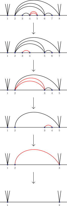
Figure C.1. Example of an allowable ordering to remove links from a planar link pattern. Notice in particular the relabeling of the indices after each step, and the fact that after each removal, the valences of the endpoints of the removed link decrease, as in Equation (C.2). Furthermore, if after the removal the endpoint becomes empty, then it is removed as well. After the removal of all the links, the defects remain.

C.2. Dual elements

Let $\omega\in\mathrm{LP}_{\varsigma}^{(s)}$ and suppose $\sigma\in\mathfrak{S}_{k}$ is an allowable ordering of the $k$ links of $\omega$ (with multiplicity), see (C.1) and Figure C.1. After removal of all the links of $\omega$ in the order $\sigma$, one is left with the link pattern $\shuffle_{\lambda(\omega)}$, which consists of $s$ defects only, determined by the partition $\lambda(\omega)$ of the defects of $\omega$ (recall Section 2.7). In terms of the vector $\mathfrak{v}_{\omega}$, the link removal can be realized as projections to subrepresentations, using the properties (3.3) of $\mathfrak{v}_{\omega}$ — since the ordering $\sigma$ is allowable, the links are removed in such a way that the removed links always connect two consecutive indices $j,j+1$.

As in Remark 3.2, we identify the one-dimensional space $\mathsf{H}_{\lambda(\omega)}^{(s)}$ with $\mathbb{C}$, via $\mathfrak{v}_{\shuffle_{\lambda(\omega)}}\mapsto 1$. This identification is implicitly used in the following definition. We set

$$\psi_{\omega}^{(\sigma)}\;\colon\;\mathsf{H}_{\varsigma}^{(s)}\to\mathbb{C},\qquad\qquad\psi_{\omega}^{(\sigma)}:=\; \tilde{\pi}_{a_{k}(k-1)}^{(\delta_{k})}\circ\cdots\circ\tilde{\pi}_{a_{2}(1)}^{(\delta_{2})}\circ\tilde{\pi}_{a_{1}}^{(\delta_{1})},$$

where

(C.2) $$\delta_{j}:=\; d_{b_{j}}^{(j-1)}+d_{a_{j}}^{(j-1)}-1-2\ell_{a_{j},b_{j}},\qquad\qquad d_{c}^{(j)}:=d_{c}-\sum_{\begin{subarray}{c}i\in\{1,2,\ldots,j\}\\ c=a_{i}\text{ or }c=b_{i}\end{subarray}}\ell_{a_{i},b_{i}}$$

so that $d_{a}^{(j)}-1$ denotes the valence of the point $a$ after removal of the $j$ links $\ell_{a_{1},b_{1}}\times\raisebox{2.15277pt}{ \scalebox{0.75}{$\underset{\;\boldsymbol{a_{1}}\;\;\boldsymbol{b_{1}}}{\vbox{\hbox{\includegraphics[scale={0.5}]{link-0.pdf}}}}$}}$, $\ldots$, $\ell_{a_{j},b_{j}}\times\raisebox{2.15277pt}{ \scalebox{0.75}{$\underset{\;\boldsymbol{a_{j}}\;\;\boldsymbol{b_{j}}}{\vbox{\hbox{\includegraphics[scale={0.5}]{link-0.pdf}}}}$}}$ from $\omega$ in the order $\sigma$, and $a_{j}(j-1)$ denotes the relabeled endpoint of the $j$:th link $\underset{\;\boldsymbol{a_{j}}\;\;\boldsymbol{b_{j}}}{\vbox{\hbox{\includegraphics[scale={0.5}]{link-0.pdf}}}}$ after removal of the $j-1$ links $\ell_{a_{1},b_{1}}\times\raisebox{2.15277pt}{ \scalebox{0.75}{$\underset{\;\boldsymbol{a_{1}}\;\;\boldsymbol{b_{1}}}{\vbox{\hbox{\includegraphics[scale={0.5}]{link-0.pdf}}}}$}}$, $\ldots$, $\ell_{a_{j-1},b_{j-1}}\times\raisebox{2.15277pt}{ \scalebox{0.75}{$\underset{\;\boldsymbol{a_{j-1}}\;\;\boldsymbol{b_{j-1}}}{\vbox{\hbox{\includegraphics[scale={0.5}]{link-0.pdf}}}}$}}$; see also Figure C.1.

We next show that $\psi_{\omega}^{(\sigma)}$ is in fact independent of the choice of allowable ordering $\sigma$ for $\omega$, and thus gives rise to a well-defined linear map

(C.3) $$\psi_{\omega}:=\psi_{\omega}^{(\sigma)}\;\colon\;\mathsf{H}_{\varsigma}^{(s)}\to\mathbb{C},$$

for any choice of allowable ordering $\sigma$ of the links in $\omega$. Moreover, we show that $\left(\psi_{\omega}\right)_{\omega\in\mathrm{LP}^{(s)}_{\varsigma}}$ is a basis of the dual space $(\mathsf{H}_{\varsigma}^{(s)})^{*}$, namely the (unnormalized) dual basis of $\left(\mathfrak{v}_{\omega}\right)_{\omega\in\mathrm{LP}^{(s)}_{\varsigma}}$.

Proposition C.1.

(see also [KP16, Proposition 3.7])

(a):

Let $\omega\in\mathrm{LP}^{(s)}_{\varsigma}$. For any two allowable orderings $\sigma$ and $\sigma^{\prime}$ of the links in $\omega$, we have

$$\psi_{\omega}^{(\sigma)}=\psi_{\omega}^{(\sigma^{\prime})}.$$

Thus, the linear functional $\psi_{\omega}\in(\mathsf{H}_{\varsigma}^{(s)})^{*}$ in (C.3) is well-defined.

(b):

For any $\omega,\tau\in\mathrm{LP}^{(s)}_{\varsigma}$, we have

(C.4) $$\psi_{\omega}(\mathfrak{v}_{\tau})=\mathrm{const.}\times\delta_{\omega,\tau},\qquad\text{where}\qquad\delta_{\omega,\tau}=\; \begin{cases}1\quad&\text{if }\tau=\omega\\ 0&\text{if }\tau\neq\omega,\end{cases}$$

and the constant is non-zero and depends only on $\omega$.

In particular, $\left(\psi_{\omega}\right)_{\omega\in\mathrm{LP}^{(s)}_{\varsigma}}$ is a basis of the dual space $(\mathsf{H}_{\varsigma}^{(s)})^{*}$.

Proof.

We use the notations introduced in Equation (C.2). Let $\omega,\tau\in\mathrm{LP}_{\varsigma}^{(s)}$, and let $\sigma$ be any allowable ordering of the links of $\omega$. Consider $\psi_{\omega}^{(\sigma)}(\mathfrak{v}_{\tau})$. If $\tau=\omega$, then by the projection property (3.3), we have

$$\tilde{\pi}_{a_{1}}^{(\delta_{1})}(\mathfrak{v}_{\omega})=\frac{1}{\mathcal{C}({\ell_{a_{1},b_{1}};s_{b_{1}},s_{a_{1}}})}\times\mathfrak{v}_{\omega/(\ell_{a_{1},b_{1}}\times\raisebox{1.50694pt}{ \scalebox{0.75}{$\underset{\;\boldsymbol{a_{1}}\;\;\boldsymbol{b_{1}}}{\vbox{\hbox{\includegraphics[scale={0.5}]{link-0.pdf}}}}$}})},$$

and recursively,

$$\Big{(}\tilde{\pi}_{a_{j}(j-1)}^{(\delta_{j})}\circ\cdots\circ\tilde{\pi}_{a_{2}(1)}^{(\delta_{2})}\circ\tilde{\pi}_{a_{1}}^{(\delta_{1})}\Big{)}(\mathfrak{v}_{\omega})=\mathrm{const.}\times\mathfrak{v}_{\omega/(\ell_{a_{1},b_{1}}\times\raisebox{1.50694pt}{ \scalebox{0.75}{$\underset{\;\boldsymbol{a_{1}}\;\;\boldsymbol{b_{1}}}{\vbox{\hbox{\includegraphics[scale={0.5}]{link-0.pdf}}}}$}})/\cdots/(\ell_{a_{j},b_{j}}\times\raisebox{1.50694pt}{ \scalebox{0.75}{$\underset{\;\boldsymbol{a_{j}}\;\;\boldsymbol{b_{j}}}{\vbox{\hbox{\includegraphics[scale={0.5}]{link-0.pdf}}}}$}})},$$

for a non-zero constant which is a product of the constants appearing in the projection properties (3.3).

For $j=k$, the above formula gives $\psi_{\omega}^{(\sigma)}(\mathfrak{v}_{\omega})=\mathrm{const.}\times\mathfrak{v}_{\shuffle_{\lambda(\omega)}}$, which we identify with the constant times $1\in\mathbb{C}$, via $\mathfrak{v}_{\shuffle_{\lambda(\omega)}}\mapsto 1$, as in Remark 3.2. On the other hand, if $\tau\neq\omega$, then for some $j$, the link pattern $\tau$ does not contain $\ell_{a_{j},b_{j}}$ links $\underset{\;\boldsymbol{a_{j}}\;\;\boldsymbol{b_{j}}}{\vbox{\hbox{\includegraphics[scale={0.5}]{link-0.pdf}}}}$ , and by the property (3.3) we then similarly get $\psi_{\omega}^{(\sigma)}(\mathfrak{v}_{\tau})=0$. Summarizing, we have $\psi_{\omega}(\mathfrak{v}_{\tau})=\mathrm{const.}\times\delta_{\omega,\tau}$, independently of the choice of allowable ordering $\sigma$, and the constant is non-zero and only depends on $\omega$. This proves Equation (C.4) and assertion (b).

By Proposition 3.7, the vectors $\mathfrak{v}_{\tau}$, with $\tau\in\mathrm{LP}_{\varsigma}^{(s)}$, form a basis of the space $\mathsf{H}_{\varsigma}^{(s)}$. It thus follows from Equation (C.4) that the value of the operator $\psi_{\omega}^{(\sigma)}$ is independent of the choice of an allowable ordering $\sigma$ of the links, and that $\left(\psi_{\omega}\right)_{\omega\in\mathrm{LP}^{(s)}_{\varsigma}}$ is a basis of the dual space $(\mathsf{H}_{\varsigma}^{(s)})^{*}$. This concludes the proof. ∎

Remark C.2.

For fixed $\omega$, by Theorem 3.1(b), the maps $\psi_{\omega}\colon\mathsf{H}_{\varsigma}^{(s)}\to\mathbb{C}$ also define (unnormalized) projectors

$$\widehat{\psi}_{\omega}\;\colon\;\bigotimes_{i=1}^{p}\mathsf{M}_{d_{i}}\to\mathsf{M}_{d},\qquad\widehat{\psi}_{\omega}(F^{l}.\mathfrak{v}_{\tau}):=\; \begin{cases}\psi_{\omega}(\mathfrak{v}_{\tau})\times e_{l}^{(d)},\quad\text{ for any }l\in\{0,1,\ldots,s\}\quad&\text{if }\tau\in\mathrm{LP}^{(s)}_{\varsigma}\\ 0&\text{otherwise,}\end{cases}$$

from the tensor product (2.5) onto the $s+1=d$-dimensional irreducible representation $\mathsf{M}_{d}$ of $\mathcal{U}_{q}(\mathfrak{sl}_{2})$. For a chosen $\upsilon\in\mathrm{LP}^{(s)}_{\varsigma}$, combining $\widehat{\psi}_{\omega}$ with the embedding $\mathsf{M}_{d}\hookrightarrow\bigotimes_{i=1}^{p}\mathsf{M}_{d_{i}}$ given by $e_{l}^{(d)}\mapsto F^{l}.\mathfrak{v}_{\upsilon}$, we can define the (unnormalized) projectors

$$\widetilde{\psi}_{\omega}^{\upsilon}\;\colon\;\bigotimes_{i=1}^{p}\mathsf{M}_{d_{i}}\to\bigotimes_{i=1}^{p}\mathsf{M}_{d_{i}},\qquad\widetilde{\psi}_{\omega}^{\upsilon}(F^{l}.\mathfrak{v}_{\tau}):=\; \begin{cases}\psi_{\omega}(\mathfrak{v}_{\tau})\times F^{l}.\mathfrak{v}_{\upsilon},\quad\text{ for any }l\in\{0,1,\ldots,s\}\quad&\text{if }\tau\in\mathrm{LP}^{(s)}_{\varsigma}\\ 0&\text{otherwise,}\end{cases}$$

onto the subrepresentations of the tensor product (2.5) isomorphic to $\mathsf{M}_{d}$, generated by $\mathfrak{v}_{\upsilon}$. This gives rise to $\sum_{s\geq 0}(\#\mathrm{LP}_{\varsigma}^{(s)})^{2}$ linearly independent maps $\widetilde{\psi}_{\omega}^{\upsilon}$, with $\omega,\upsilon\in\mathrm{LP}^{(s)}_{\varsigma}$, that belong to the commutant algebra $\mathrm{End}_{\mathcal{U}_{q}(\mathfrak{sl}_{2})}\big{(}\bigotimes_{i=1}^{p}\mathsf{M}_{d_{i}}\big{)}$. We discuss this commutant algebra in forthcoming work [FP20a⁺].

C.3. Some details for the proofs of Lemma 5.5 and Proposition 5.6

Let $1\leq j<k\leq p$ and $\omega\in\mathrm{LP}^{(s)}_{\varsigma}$, and let $\tau\in\mathrm{LP}_{\varsigma_{j,k}}^{(r)}$ be the sub-link pattern of $\omega$ with index valences $\varsigma_{j,k}=(s_{j},s_{j+1}\ldots,s_{k})$, consisting of the lines of $\omega$ attached to the indices $j,j+1,\ldots,k$, as in Section 5.3, and let $\omega/\tau$ denote the link pattern obtained from $\omega$ by “removing $\tau$”, that is, removing from $\omega$ the links $\underset{\;\boldsymbol{a\;}\;\;\boldsymbol{\;b\,}}{\vbox{\hbox{\includegraphics[scale={0.5}]{link-0.pdf}}}}$ with indices $a,b\in\{j,j+1,\ldots,k\}$, collapsing the indices $j,j+1,\ldots,k$ of $\omega$ into one point, and relabeling the indices thus obtained from left to right by $1,2,\ldots$ (see Section 5.3).

Lemma C.3.

Let $\omega\in\mathrm{LP}_{\varsigma}^{(s)}$, $\tau\in\mathrm{LP}_{\varsigma_{j,k}}^{(r)}$, and $\omega/\tau$ be as in Section 5.3. Then we have

$$\mathfrak{v}_{\omega}=\; \sum_{l=0}^{r}\sum_{\begin{subarray}{c}l_{1},\ldots,l_{j-1},\\ l_{k+1},\ldots,l_{p}\end{subarray}}c_{l_{1},\ldots,l_{j-1};l;l_{k+1},\ldots,l_{p}}\times\left(e_{l_{p}}\otimes\cdots\otimes e_{l_{k+1}}\otimes F^{l}.\mathfrak{v}_{\tau}\otimes e_{l_{j-1}}\otimes\cdots\otimes e_{l_{1}}\right)$$

$$\mathfrak{v}_{\omega/\tau}=\; \sum_{l=0}^{r}\sum_{\begin{subarray}{c}l_{1},\ldots,l_{j-1},\\ l_{k+1},\ldots,l_{p}\end{subarray}}c_{l_{1},\ldots,l_{j-1};l;l_{k+1},\ldots,l_{p}}\times\left(e_{l_{p}}\otimes\cdots\otimes e_{l_{k+1}}\otimes e_{l}\otimes e_{l_{j-1}}\otimes\cdots\otimes e_{l_{1}}\right),$$

for some constants $c_{l_{1},\ldots,l_{j-1};l;l_{k+1},\ldots,l_{p}}\in\mathbb{C}$.

Proof.

By Theorem 3.1(b), the vector $\mathfrak{v}_{\omega}$ can be written as a linear combination

$$\mathfrak{v}_{\omega}=\sum_{t\geq 0}\sum_{\upsilon\in\mathrm{LP}^{(t)}_{\varsigma_{j,k}}}\sum_{l=0}^{t}\sum_{\begin{subarray}{c}l_{1},\ldots,l_{j-1},\\ l_{k+1},\ldots,l_{p}\end{subarray}}c^{t,\upsilon}_{l_{1},\ldots,l_{j-1};l;l_{k+1},\ldots,l_{p}}\times\left(e_{l_{p}}\otimes\cdots\otimes e_{l_{k+1}}\otimes F^{l}.\mathfrak{v}_{\upsilon}\otimes e_{l_{j-1}}\otimes\cdots\otimes e_{l_{1}}\right),$$

for some constants $c^{t,\upsilon}_{l_{1},\ldots,l_{j-1};l;l_{k+1},\ldots,l_{p}}\in\mathbb{C}$. For any $\upsilon\in\mathrm{LP}^{(t)}_{\varsigma_{j,k}}$, we apply the map

$$(\widehat{\psi}_{\upsilon})_{j,k}=\mathrm{id}^{\otimes(p-k)}\otimes\widehat{\psi}_{\upsilon}\otimes\mathrm{id}^{\otimes(j-1)}\;\colon\;\bigotimes_{i=1}^{p}\mathsf{M}_{d_{i}}\;\longrightarrow\;(\mathsf{M}_{d_{p}}\otimes\cdots\otimes\mathsf{M}_{d_{k+1}})\otimes\mathsf{M}_{t+1}\otimes(\mathsf{M}_{d_{j-1}}\otimes\cdots\otimes\mathsf{M}_{d_{1}})$$

to both sides of the above expression for $\mathfrak{v}_{\omega}$. By the projection properties (3.3) of $\mathfrak{v}_{\omega}$, the vector $(\widehat{\psi}_{\upsilon})_{j,k}(\mathfrak{v}_{\omega})$ equals zero unless $\upsilon=\tau$, and if $\upsilon=\tau$, then we have $(\widehat{\psi}_{\tau})_{j,k}(\mathfrak{v}_{\omega})=\psi_{\tau}(\mathfrak{v}_{\tau})\times\mathfrak{v}_{\omega/\tau}$, by similar arguments as in the proof of Proposition C.1. Analogous properties hold for $(\widetilde{\psi}_{\upsilon}^{\upsilon})_{j,k}$, which picks the component generated by $\mathfrak{v}_{\upsilon}$ in the tensor positions $j,j+1,\ldots,k$. Therefore, we have

$$\mathfrak{v}_{\omega}=\sum_{l=0}^{r}\sum_{\begin{subarray}{c}l_{1},\ldots,l_{j-1},\\ l_{k+1},\ldots,l_{p}\end{subarray}}c_{l_{1},\ldots,l_{j-1};l;l_{k+1},\ldots,l_{p}}\times\left(e_{l_{p}}\otimes\cdots\otimes e_{l_{k+1}}\otimes F^{l}.\mathfrak{v}_{\tau}\otimes e_{l_{j-1}}\otimes\cdots\otimes e_{l_{1}}\right),$$

where $c_{l_{1},\ldots,l_{j-1};l;l_{k+1},\ldots,l_{p}}=c^{r,\tau}_{l_{1},\ldots,l_{j-1};l;l_{k+1},\ldots,l_{p}}$, and in particular,

$$\mathfrak{v}_{\omega/\tau}=\sum_{l=0}^{r}\sum_{\begin{subarray}{c}l_{1},\ldots,l_{j-1},\\ l_{k+1},\ldots,l_{p}\end{subarray}}c_{l_{1},\ldots,l_{j-1};l;l_{k+1},\ldots,l_{p}}\times\left(e_{l_{p}}\otimes\cdots\otimes e_{l_{k+1}}\otimes e_{l}\otimes e_{l_{j-1}}\otimes\cdots\otimes e_{l_{1}}\right).$$

∎

References

- [BB03a] M. Bauer and D. Bernard. Conformal field theories of stochastic Loewner evolutions. Comm. Math. Phys., 239(3):493–521, 2003.
- [BB03b] M. Bauer and D. Bernard. , CFT and zig-zag probabilities. In Proceedings of the conference ‘Conformal Invariance and Random Spatial Processes’, Edinburgh, 2003.
- [BBK05] M. Bauer, D. Bernard, and K. Kytölä. Multiple Schramm-Loewner evolutions and statistical mechanics martingales. J. Stat. Phys., 120(5-6):1125–1163, 2005.
- [BFIZ91] M. Bauer, P. Di Francesco, C. Itzykson, and J. B. Zuber. Covariant differential equations and singular vectors in Virasoro representations. Nuclear Phys. B, 362(3):515–562, 1991.
- [BJV13] D. Beliaev and F. Johansson-Viklund. Some remarks on bubbles and Schramm’s two-point observable. Comm. Math. Phys., 320(2):379–394, 2013.
- [Bon69] J. M. Bony. Principe du maximum, inégalite de Harnack et unicité du problème de Cauchy pour les opérateurs elliptiques dégénérés. Ann. Inst. Fourier (Grenoble), 19(1):277–304, 1969.
- [BPZ84a] A. A. Belavin, A. M. Polyakov, and A. B. Zamolodchikov. Infinite conformal symmetry in two-dimensional quantum field theory. Nuclear Phys. B, 241(2):333–380, 1984.
- [BPZ84b] A. A. Belavin, A. M. Polyakov, and A. B. Zamolodchikov. Infinite conformal symmetry of critical fluctuations in two dimensions. J. Stat. Phys., 34(5-6):763–774, 1984.
- [BPW18] V. Beffara, E. Peltola, and H. Wu. On the uniqueness of global multiple s. Preprint in arXiv:1801.07699, 2018.
- [BSA88] L. Benoit and Y. Saint-Aubin. Degenerate conformal field theories and explicit expressions for some null vectors. Phys. Lett. B, 215(3):517–522, 1988.
- [Car84] J. L. Cardy. Conformal invariance and surface critical behavior. Nuclear Phys. B, 240(4):514–532, 1984.
- [Car89] J. L. Cardy. Boundary conditions, fusion rules and the Verlinde formula. Nuclear Phys. B, 324(3):581–596, 1989.
- [Car92] J. L. Cardy. Critical percolation in finite geometries. J. Phys. A, 25(4):L201–206, 1992.
- [CDCH+14] D. Chelkak, H. Duminil-Copin, C. Hongler, A. Kemppainen, and S. Smirnov. Convergence of Ising interfaces to Schramm’s curves. C. R. Acad. Sci. Paris Sér. I Math., 352(2):157–161, 2014.
- [CN06] F. Camia and C. M. Newman. Two-dimensional critical percolation: the full scaling limit. Comm. Math. Phys., 268(1):1–38, 2006.
- [DF84] V. S. Dotsenko and V. A. Fateev. Conformal algebra and multipoint correlation functions in statistical models. Nuclear Phys. B, 240(3):312–348, 1984.
- [DFMS97] Philippe Di Francesco, Pierre Mathieu, and David Sénéchal. Conformal field theory. Graduate Texts in Contemporary Physics. Springer-Verlag, New York, 1997.
- [Dub06a] J. Dubédat. Euler integrals for commuting . J. Stat. Phys., 123(6):1183–1218, 2006.
- [Dub06b] J. Dubédat. Excursion decompositions for and Watts’ crossing formula. Probab. Theory Related Fields, 134(3):453–488, 2006.
- [Dub07] J. Dubédat. Commutation relations for . Comm. Pure Appl. Math., 60(12):1792–1847, 2007.
- [Dub15a] J. Dubédat. and Virasoro representations: Localization. Comm. Math. Phys., 336(2):695–760, 2015.
- [Dub15b] J. Dubédat. and Virasoro representations: Fusion. Comm. Math. Phys., 336(2):761–809, 2015.
- [Dup06] B. Duplantier. Conformal random geometry. In Mathematical Statistical Physics: Lecture Notes of the Les Houches Summer School (2005), Course 3. Elsevier, 2006.
- [FF84] B. L. Feĭgin and D. B. Fuchs. Verma modules over the Virasoro algebra. In Topology (Leningrad 1982), volume 1060 of Lecture notes in mathematics, pages 230–245. Springer-Verlag, Berlin Heidelberg, 1984.
- [FK97] I. B. Frenkel and M. G. Khovanov. Canonical bases in tensor products and graphical calculus for . Duke Math. J., 87(3):409–480, 1997.
- [FK04] R. Friedrich and J. Kalkkinen. On conformal field theory and stochastic Loewner evolution. Nuclear Phys. B, 687(3):279–302, 2004.
- [FK15a] S. M. Flores and P. Kleban. A solution space for a system of null-state partial differential equations, Part 3. Comm. Math. Phys., 333(2):597–667, 2015.
- [FK15b] S. M. Flores and P. Kleban. A solution space for a system of null-state partial differential equations, Part 4. Comm. Math. Phys., 333(2):669–715, 2015.
- [FP18] S. M. Flores and E. Peltola. Standard modules, radicals, and the valenced Temperley-Lieb algebra. Preprint in arXiv:1801.10003, 2018.
- [FP20a+] S. M. Flores and E. Peltola. Higher quantum and classical Schur-Weyl duality for . In preparation.
- [FP20b+] S. M. Flores and E. Peltola. Solution spaces for the Benoit Saint-Aubin partial differential equations. In preparation.
- [FSK15] S. M. Flores, J. J. H. Simmons, and P. Kleban. Multiple- connectivity weights for rectangles, hexagons, and octagons. Preprint in arXiv:1505.07756, 2015.
- [FW91] G. Felder and C. Wieczerkowski. Topological representations of the quantum group . Comm. Math. Phys., 138(3):583–605, 1991.
- [FW03] R. Friedrich and W. Werner. Conformal restriction, highest weight representations and . Comm. Math. Phys., 243(1):105–122, 2003.
- [GC05] A. Gamsa and J. L. Cardy. The scaling limit of two cluster boundaries in critical lattice models. J. Stat. Mech. Theory Exp., 12:P12009, 2005.
- [HK13] C. Hongler and K. Kytölä. Ising interfaces and free boundary conditions. J. Amer. Math. Soc., 26(4):1107–1189, 2013.
- [Hör67] L. Hörmander. Hypoelliptic second-order differential equations. Acta Math., 119:147–171, 1967.
- [Izy15] K. Izyurov. Smirnov’s observable for free boundary conditions, interfaces and crossing probabilities. Comm. Math. Phys., 337(1):225–252, 2015.
- [Izy17] K. Izyurov. Critical Ising interfaces in multiply-connected domains. Probab. Theory Related Fields, 167(1):379–415, 2017.
- [Jim86] M. Jimbo. A analog of , Hecke algebra and the Yang-Baxter equation. Lett. Math. Phys., 11(3):247–252, 1986.
- [JJK16] N. Jokela, M. Järvinen, and K. Kytölä. boundary visits. Ann. Henri Poincaré, 17(6):1263–1330, 2016.
- [KKP19] A. Karrila, K. Kytölä, and E. Peltola. Conformal blocks, -combinatorics, and quantum group symmetry. Ann. Inst. Henri Poincaré D, 6(3):449–487, 2019.
- [KKP20] A. Karrila, K. Kytölä, and E. Peltola. Boundary correlations in planar LERW and UST. Comm. Math. Phys., to appear. Preprint in arXiv:1702.03261.
- [KL07] M. J. Kozdron and G. F. Lawler. The configurational measure on mutually avoiding paths. Fields Inst. Commun., 50:199–224, 2007.
- [Kon87] M. L. Kontsevich. The Virasoro algebra and Teichmüller spaces. Funct. Anal. Appl., 21(2):156–157, 1987.
- [Kon03] M. L. Kontsevich. CFT, , and phase boundaries. Oberwolfach Arbeitstagung, 2003.
- [KP16] K. Kytölä and E. Peltola. Pure partition functions of multiple . Comm. Math. Phys., 346(1):237–292, 2016.
- [KP20] K. Kytölä and E. Peltola. Conformally covariant boundary correlation functions with a quantum group. J. Eur. Math. Soc., 22(1):55–118, 2020.
- [KS07] M. L. Kontsevich and Y. Suhov. On Malliavin measures, , and CFT. P. Steklov I. Math. 258(1):100–146, 2007.
- [KS18] A. Kemppainen and S. Smirnov. Configurations of FK Ising interfaces and hypergeometric SLE. Math. Res. Lett., 25(3):875–889, 2018.
- [LSW04] G. F. Lawler, O. Schramm, and W. Werner. Conformal invariance of planar loop-erased random walks and uniform spanning trees. Ann. Probab., 32(1B):939–995, 2004.
- [Lus92] G. Lusztig. Canonical bases in tensor products. Proc. Nat. Acad. Sci. U.S.A., 89:8177–8179, 1992.
- [LV19a] J. Lenells and F. Viklund. Schramm’s formula and the Green’s function for multiple . J. Stat. Phys., 176(4):873–931, 2019.
- [LV19b] J. Lenells and F. Viklund. Asymptotic analysis of Dotsenko-Fateev integrals. Ann. Henri Poincaré, 20(11):3799–3848, 2019.
- [Mar92] P. P. Martin. On Schur-Weyl duality, Hecke algebras and quantum on . Int. J. Mod. Phys. A, 7(01b):645–673, 1992.
- [PSA14] G. Provencher and Y. Saint-Aubin. The idempotents of the -module in terms of elements of . Ann. Henri Poincaré, 15(11):2203–2240, 2014.
- [PW19] E. Peltola and H. Wu. Global and local multiple s for and connection probabilities for level lines of . Comm. Math. Phys., 366(2):469–536, 2019.
- [RSA14] D. Ridout and Y. Saint-Aubin. Standard modules, induction and the structure of the Temperley-Lieb algebra. Adv. Theor. Math. Phys., 18(5):957–1041, 2014.
- [Sch00] O. Schramm. Scaling limits of loop-erased random walks and uniform spanning trees. Israel J. Math., 118(1):221–288, 2000.
- [Smi01] S. Smirnov. Critical percolation in the plane: conformal invariance, Cardy’s formula, scaling limits. C. R. Acad. Sci., 333(3):239–244, 2001. (updated 2009, see arXiv:0909.4499).
- [Smi06] S. Smirnov. Towards conformal invariance of lattice models. In Proceedings of the ICM 2006, Madrid, Spain, volume II, pages 1421–1451. European Mathematical Society, 2006.
- [SS05] O. Schramm and S. Sheffield. The harmonic explorer and its convergence to . Ann. Probab., 33(6):2127–2148, 2005.
- [SW11] S. Sheffield and D. Wilson. Schramm’s proof of Watts’ formula. Ann. Probab. 39(5):1844–1863, 2011.
- [Wat96] G. Watts. A crossing probability for critical percolation in two dimensions. J. Phys. A, 29:L363, 1996.
- [Zha08] D. Zhan. The scaling limits of planar LERW in finitely connected domains. Ann. Probab., 36(2):467–529, 2008.