Efficient Algorithms for Time- and
Cost-Bounded Probabilistic Model Checking

Abstract

In the design of probabilistic timed systems, bounded requirements concerning behaviour that occurs within a given time, energy, or more generally cost budget are of central importance. Traditionally, such requirements have been model-checked via a reduction to the unbounded case by unfolding the model according to the cost bound. This exacerbates the state space explosion problem and significantly increases runtime. In this paper, we present three new algorithms to model-check time- and cost-bounded properties for Markov decision processes and probabilistic timed automata that avoid unfolding. They are based on a modified value iteration process, on an enumeration of schedulers, and on state elimination techniques. We can now obtain results for any cost bound on a single state space no larger than for the corresponding unbounded or expected-value property. In particular, we can naturally compute the cumulative distribution function at no overhead. We evaluate the applicability and compare the performance of our new algorithms and their implementation on a number of case studies from the literature.

1 Introduction

Markov decision processes (MDP, [21]) and probabilistic timed automata (PTA, [19]) are two popular formal models for probabilistic (real-time) systems. The former combine nondeterministic choices, which can be due to concurrency, unquantified uncertainty, or abstraction, with discrete probabilistic decisions, which represent quantified uncertainty e.g. due to environmental influences or in randomised algorithms. The latter additionally provide facilities to model hard real-time behaviour and constraints as in timed automata. Given an MDP or a PTA, queries like “what is the worst-case probability to reach an unsafe system state” or “what is the minimum expected time to termination” can be answered via probabilistic model checking [3, 20]. Although limited by the state space explosion problem, it works well on relevant case studies.

In practice, an important class of queries relates to cost- or reward-bounded properties, such as “what is the probability of a message to arrive after at most three transmission attempts” in a communication protocol, or “what is the expected energy consumption within the first five hours after waking from sleep” in a battery-powered device. Costs and rewards are the same concept, and we will prefer the term reward in the remainder of this paper. In the properties above, we have three different rewards: retransmission attempts (accumulating reward 1 for each attempt), energy consumption (accumulating reward at a state-dependent wattage), and time (accumulating reward at a rate of 1 in all states). To compute reward-bounded properties, the traditional approach for discrete-time probabilistic models is to unfold the state space [2]: in addition to the current state of the model, one keeps track of the reward accumulated so far, up to the specified bound value $b\in\mathbb{N}$ (e.g. $b=3$ in the first property above). This blows up the size of the state space linearly in $b$, and often causes the model checking process to run out of memory. The situation for PTA is no different: the bounded case is reduced to the unbounded one by extending the model, e.g. by adding a new clock variable that is never reset to check time-bounded properties [20], with the same effect on state space size. Using a digital clocks semantics [18], the analysis of PTA with rewards can be reduced to MDP model checking.

In this paper, we present three new algorithms for probabilistic model checking of reward-bounded properties without unfolding. The first algorithm is a modification of standard unbounded value iteration. The other algorithms use different techniques—scheduler enumeration with either value iteration or Markov chain state elimination, and MDP state elimination—to reduce the model such that all remaining transitions correspond to accumulating a reward of $1$. A reward-bounded property with bound $b$ in the original model then corresponds to a step-bounded property with bound $b$ in the reduced model. We use standard step-bounded value iteration [21] to check these properties efficiently.

Common to all three algorithms is that there is no blowup in the number of states due to unfolding. There no blowup at all in the first algorithm. If we could previously check an unbounded property with a given amount of memory, we can now check the corresponding bounded property for any bound value $b$, too. In fact, when asked for the probability to reach a certain set of states with accumulated reward $\leq b$, all three algorithms actually compute the sequence of probabilities for bounds $0,\dots,b$. At no overhead, we thus obtain the cumulative (sub)distribution function over the bound up to $b$. If it converges in a finite number of steps, then we can detect this step by keeping track of the maximum error in the value iterations. We may thus obtain the entire function without the user having to specify an a priori bound. From a practical perspective, this means that with memory previously sufficient to compute the (unbounded) expected reward (i.e. the mean or first moment of the underlying distribution), we can now obtain the entire distribution (i.e. all moments). Domain experts may accept a mean as a good first indicator of a system’s behaviour, but are ultimately more interested in the actual shape of the distribution as a whole.

We have implemented all three algorithms in the mcsta tool, which is available as part of the Modest Toolset [11]. After describing the algorithms in Sect. 3 and the implementation in Sect. 4, we use a number of case studies from the literature to evaluate the applicability and performance in Sect. 5.

Related work.

Only very recently has a procedure to handle reward-bounded properties without unfolding been described for MDP [3, 13]. It works by solving a sequence of linear programming problems. Solution vectors need to be stored to solve the subsequent instances. Linear programming does not scale to large MDP, and we are not currently aware of a publicly available implementation of this procedure. Yet, the underlying idea is similar to the first algorithm that we present in this paper, which uses value iteration instead. For the soft real-time model of Markov automata, which includes MDP as a special case, reward-bounded properties can be turned into time-bounded ones [14]. However, this only works for rewards associated to Markovian states, whereas immediate states (i.e. the MDP subset of Markov automata) always implicitly get zero reward.

2 Preliminaries

$\mathbb{N}$ is $\{\,0,1,\dots\,\}$, the set of natural numbers. $\mathbb{Q}^{+}$ is the set of positive rational numbers. $\mathbb{R}^{+}_{0}$ is $[0,\infty)$, the set of nonnegative real numbers. $2^{S}$ denotes the powerset of $S$. $\mathrm{Dom}({f})$ is the domain of the function $f$.

Definition 1

A (discrete) probability distribution over a set $\varOmega$ is a function $\mu\in\varOmega\to[0,1]$ such that $\mathrm{support}({\mu})\mathrel{\vbox{\offinterlineskip\halign{\hfil#\hfil\cr{\tiny\rm def}\cr\kern 1.29167pt\cr$=$\cr}}}\{\,\omega\in\varOmega\mid\mu(\omega)>0\,\}$ is countable and $\sum_{\omega\in\mathrm{support}({\mu})}{\mu(\omega)}=1$. $\mathrm{Dist}({\varOmega})$ is the set of all probability distributions over $\varOmega$. $\mathcal{D}(s)$ is the Dirac distribution for $s$, defined by $\mathcal{D}(s)(s)=1$.

2.0.1 Markov Decision Processes

To move from one state to another in a Markov decision process, first a transition is chosen nondeterministically; each transition then leads into a probability distribution over successor states.

Definition 2

A Markov decision process (MDP) is a tuple $M=\langle S,A,T,s_{\mathit{init}}\rangle$ where $S$ is a finite set of states, $A$ is a finite set of actions, $T\in S\to 2^{A\times\mathrm{Dist}({S})}$ is the transition function, and $s_{\mathit{init}}\in S$ is the initial state. For all $s\in S$, we require that $T(s)$ is finite non-empty, and that if $\langle a,\mu\rangle\in T(s)$ and $\langle a,\mu^{\prime}\rangle\in T(s)$ then $\mu=\mu^{\prime}$. We call $s\in S$ deterministic if $|T(s)|=1$.

We write $s\xrightarrow{{\raisebox{-1.5pt}[0.0pt][0.0pt]{$\scriptstyle{a}$}}}_{T}\mu$ for $\exists\,a,\mu\colon\langle a,\mu\rangle\in T(s)$ and call it a transition. We write $s\xrightarrow{{\raisebox{-1.5pt}[0.0pt][0.0pt]{$\scriptstyle{a}$}}}_{T}s^{\prime}$ if additionally $s^{\prime}\in\mathrm{support}({\mu})$. If $T$ is clear from the context, we write $\xrightarrow{{\raisebox{-1.5pt}[0.0pt][0.0pt]{$\scriptstyle{}$}}}$ instead of $\xrightarrow{{\raisebox{-1.5pt}[0.0pt][0.0pt]{$\scriptstyle{}$}}}_{T}$. Graphically, we represent transitions as action-labelled lines to an intermediate node from which weighted branches lead to successor states. We may omit action labels out of deterministic states as well as the intermediate node and probability $1$ for transitions into Dirac distributions.

Definition 3

A reward structure for $M$ is a function $\mathit{Rew}\in S\times A\times S\to\mathbb{R}^{+}_{0}$ such that $\mathit{Rew}(\langle s,a,s^{\prime}\rangle)\neq 0\mathrel{\Rightarrow}s\xrightarrow{{\raisebox{-1.5pt}[0.0pt][0.0pt]{$\scriptstyle{a}$}}}s^{\prime}$. It associates a branch reward to each choice of action and successor state for all transitions.

Figure 1: Example MDP $M^{e}$

Figure 2: Transformed MDP ${{M^{e}}{\downarrow}_{F^{e}}}{\downarrow}_{\mathit{Rew}^{e}}$

Fig. 2 shows an example MDP $M^{e}$ with 5 states, 6 transitions and 10 branches. States $u$, $v$ and $w$ are deterministic. $M^{e}$ has one reward structure $\mathit{Rew}^{e}$ with $\mathit{Rew}^{e}(\langle s,\texttt{b},s\rangle)=\mathit{Rew}^{e}(\langle t,\texttt{d},t\rangle)=1$ and $\mathit{Rew}^{e}(\mathit{tr})=0$ otherwise.

Using MDP directly to build complex models is cumbersome. Instead, high-level formalisms such as Prism’s [16] guarded command language are used. Aside from a parallel composition operator, they extend MDP with variables over finite domains that can be used in expressions to e.g. enable/disable transitions. The semantics of such a high-level model is an MDP whose states are the valuations of the variables. This allows to compactly describe very large MDP.

Paths and schedulers.

The semantics of an MDP $M=\langle S,A,T,s_{\mathit{init}}\rangle$ is captured by the notion of paths. A path represents a concrete resolution of both nondeterministic and probabilistic choices:

Definition 4

A finite path from $s_{0}$ to $s_{n}$ of length $n\in\mathbb{N}$ is a finite sequence $\pi_{\mathrm{fin}}=s_{0}\,a_{0}\,s_{1}\,a_{1}\,s_{2}\dots a_{n-1}\,s_{n}$ where $s_{i}\in S$ for all $i\in\{\,0,\dots,n\,\}$ and $s_{i}\xrightarrow{{\raisebox{-1.5pt}[0.0pt][0.0pt]{$\scriptstyle{a_{i}}$}}}s_{i+1}$ for all $i\in\{\,0,\dots,n-1\,\}$. Let $|\pi_{\mathrm{fin}}|\mathrel{\vbox{\offinterlineskip\halign{\hfil#\hfil\cr{\tiny\rm def}\cr\kern 1.29167pt\cr$=$\cr}}}n$ and $\mathrm{last}(\pi_{\mathrm{fin}})\mathrel{\vbox{\offinterlineskip\halign{\hfil#\hfil\cr{\tiny\rm def}\cr\kern 1.29167pt\cr$=$\cr}}}s_{n}$. Given a reward structure $\mathit{Rew}$, we define $\mathrm{reward}(\mathit{Rew},\pi_{\mathrm{fin}})=\sum_{i=0}^{n-1}\mathit{Rew}(\langle s_{i},a_{i},s_{i+1}\rangle)$. $\mathrm{Paths}_{\mathrm{fin}}(M)$ is the set of all finite paths from $s_{\mathit{init}}$. An (infinite) path starting from $s_{0}$ is an infinite sequence $\pi=s_{0}\,a_{0}\,s_{1}\,a_{1}\,s_{2}\dots$ where for all $i\in\mathbb{N}$, we have that $s_{i}\in S$ and $s_{i}\xrightarrow{{\raisebox{-1.5pt}[0.0pt][0.0pt]{$\scriptstyle{a_{i}}$}}}s_{i+1}$. $\mathrm{Paths}(M)$ is the set of all infinite paths starting from $s_{\mathit{init}}$. Given a set $F\subseteq S$, let $\pi^{\diamond F}$ be the shortest prefix of $\pi$ that contains a state in $F$, or $\bot$ if such a prefix does not exist.

In contrast to a path, a scheduler (or adversary, policy or strategy) only resolves the nondeterministic choices of $M$:

Definition 5

A scheduler is a function $\mathfrak{S}\in\mathrm{Paths}_{\mathrm{fin}}(M)\to\mathrm{Dist}({A})$ such that $\forall\,s\in S\colon a\in\mathrm{support}({\mathfrak{S}(s)})\mathrel{\Rightarrow}s\xrightarrow{{\raisebox{-1.5pt}[0.0pt][0.0pt]{$\scriptstyle{a}$}}}\mu$. $\mathrm{Sched}(M)$ is the set of all schedulers of $M$. $\mathfrak{S}$ is reward-positional for a reward structure $\mathit{Rew}$ if $\mathrm{last}(\pi_{1})=\mathrm{last}(\pi_{2})$ and $\mathrm{reward}(\mathit{Rew},\pi_{1})=\mathrm{reward}(\mathit{Rew},\pi_{2})$ implies $\mathfrak{S}(\pi_{1})=\mathfrak{S}(\pi_{2})$, positional if $\mathrm{last}(\pi_{1})=\mathrm{last}(\pi_{2})$ alone implies $\mathfrak{S}(\pi_{1})=\mathfrak{S}(\pi_{2})$, and deterministic if $|\mathrm{support}({\mathfrak{S}(\pi)})|=1$, for all finite paths $\pi$, $\pi_{1}$ and $\pi_{2}$, respectively. A simple scheduler is positional and deterministic. It can thus be seen as a function in $S\to A$. The set of all simple schedulers of $M$ is $\mathrm{SSched}(M)$.

Let ${M}{\downarrow}_{\mathfrak{S}_{\mathrm{s}}}\mathrel{\vbox{\offinterlineskip\halign{\hfil#\hfil\cr{\tiny\rm def}\cr\kern 1.29167pt\cr$=$\cr}}}\langle S,A,T^{\prime},s_{\mathit{init}}\rangle$ with $T^{\prime}(s)\mathrel{\vbox{\offinterlineskip\halign{\hfil#\hfil\cr{\tiny\rm def}\cr\kern 1.29167pt\cr$=$\cr}}}\{\,\langle a,\mu\rangle\mid s\xrightarrow{{\raisebox{-1.5pt}[0.0pt][0.0pt]{$\scriptstyle{a}$}}}\mu\wedge\mathfrak{S}_{\mathrm{s}}(s)=a\,\}$ for $\mathfrak{S}_{\mathrm{s}}\in\mathrm{SSched}(M)$. All states in ${M}{\downarrow}_{\mathfrak{S}_{\mathrm{s}}}$ are deterministic, i.e. ${M}{\downarrow}_{\mathfrak{S}_{\mathrm{s}}}$ is a discrete-time Markov chain (DTMC). Using the standard cylinder set construction [4], a scheduler $\mathfrak{S}$ induces a probability measure $\mathcal{P}^{\mathfrak{S}}_{M}$ on measurable sets of paths starting from $s_{\mathit{init}}$. Let $\mathcal{E}^{\mathfrak{S}}_{M}(\mathit{rv})$ denote the expectation of random variable $\mathit{rv}$ under this probability measure. We define the extremal values $\mathcal{P}^{\mathrm{max}}_{M}(\Pi)=\sup_{\mathfrak{S}\in\mathrm{Sched}(M)}\mathcal{P}^{\mathfrak{S}}_{M}(\Pi)$ and $\mathcal{P}^{\mathrm{min}}_{M}(\Pi)=\inf_{\mathfrak{S}\in\mathrm{Sched}(M)}\mathcal{P}^{\mathfrak{S}}_{M}(\Pi)$. For expectations, $\mathcal{E}^{\mathrm{max}}_{M}$ and $\mathcal{E}^{\mathrm{min}}_{M}$ are defined analogously.

Properties.

For an MDP $M$, reward structures $\mathit{Rew}_{\mathrm{exp}}$ and $\mathit{Rew}_{\mathrm{bound}}$, and a set of goal states $F\subseteq S$, we define the following values for $\mathit{opt}\in\{\,\mathrm{max},\mathrm{min}\,\}$:

• $\mathrm{P}_{\!{\mathit{opt}}}({F})$ is the extremal probability of eventually reaching $F$, defined as $\mathcal{P}^{\mathit{opt}}_{M}(\Pi)$ where $\Pi$ is the set of paths in $\mathrm{Paths}(M)$ that contain a state in $F$.

• $\mathrm{P}^{\mathrm{T}[\leq{n}]}_{\!{\mathit{opt}}}({F})$ is the extremal probability of reaching $F$ via at most $n\in\mathbb{N}$ transitions, defined as $\mathcal{P}^{\mathit{opt}}_{M}(\Pi^{\mathrm{T}}_{n})$ where $\Pi^{\mathrm{T}}_{n}$ is the set of paths that have a prefix of length at most $n$ that contains a state in $F$.

• $\mathrm{P}^{\mathrm{R}[\leq{n}]}_{\!{\mathit{opt}}}({F})$ is the extremal probability of reaching $F$ with accumulated reward $\mathit{Rew}_{\mathrm{bound}}$ at most $n\in\mathbb{R}$, defined as $\mathcal{P}^{\mathit{opt}}_{M}(\Pi^{\mathrm{R}}_{n})$ where $\Pi^{\mathrm{R}}_{n}$ is the set of paths that have a prefix $\pi_{\mathrm{fin}}$ containing a state in $F$ with $\mathrm{reward}(\mathit{Rew}_{\mathrm{bound}},\pi_{\mathrm{fin}})\leq n$.

• $\mathrm{R}_{\!{\mathit{opt}}}({F})$ is the expected accumulated reward $\mathit{Rew}_{\mathrm{exp}}$ when reaching a state in $F$, defined as $\mathcal{E}^{\mathit{opt}}_{M}(f(F))$ where $f(F)(\pi)\mathrel{\vbox{\offinterlineskip\halign{\hfil#\hfil\cr{\tiny\rm def}\cr\kern 1.29167pt\cr$=$\cr}}}\mathrm{reward}(\mathit{Rew}_{\mathrm{exp}},\pi^{\diamond F})$ for $\pi^{\diamond F}\neq\bot$ and $f(F)(\bot)\mathrel{\vbox{\offinterlineskip\halign{\hfil#\hfil\cr{\tiny\rm def}\cr\kern 1.29167pt\cr$=$\cr}}}\infty$,

• $\mathrm{R}^{\mathrm{T}[\leq{n}]}_{\!{\mathit{opt}}}({F})$ is the expected accumulated reward $\mathit{Rew}_{\mathrm{exp}}$ when reaching a state in $F$ via at most $n\in\mathbb{N}$ transitions, defined as $\mathcal{E}^{\mathit{opt}}_{M}(f^{T}_{n}(F))$ where $f^{T}_{n}(F)(\pi)\mathrel{\vbox{\offinterlineskip\halign{\hfil#\hfil\cr{\tiny\rm def}\cr\kern 1.29167pt\cr$=$\cr}}}\mathrm{reward}(\mathit{Rew}_{\mathrm{exp}},\pi^{\diamond F})$ if $\pi^{\diamond F}\neq\bot\wedge|\pi^{\diamond F}|\leq n$ and $f(F)(\pi)\mathrel{\vbox{\offinterlineskip\halign{\hfil#\hfil\cr{\tiny\rm def}\cr\kern 1.29167pt\cr$=$\cr}}}\infty$ otherwise.

• $\mathrm{R}^{\mathrm{R}[\leq{n}]}_{\!{\mathit{opt}}}({F})$ is the expected accumulated reward $\mathit{Rew}_{\mathrm{exp}}$ when reaching $F$ with accumulated reward $\mathit{Rew}_{\mathrm{bound}}$ at most $n\in\mathbb{R}$, defined as $\mathcal{E}^{\mathit{opt}}_{M}(f^{R}_{n}(F))$ where $f^{R}_{n}(F)(\pi)\mathrel{\vbox{\offinterlineskip\halign{\hfil#\hfil\cr{\tiny\rm def}\cr\kern 1.29167pt\cr$=$\cr}}}\mathrm{reward}(\mathit{Rew}_{\mathrm{exp}},\pi^{\diamond F})$ if $\pi^{\diamond F}\neq\bot\wedge\mathrm{reward}(\mathit{Rew}_{\mathrm{bound}},\pi^{\diamond F})\leq n$ and $f(F)(\pi)\mathrel{\vbox{\offinterlineskip\halign{\hfil#\hfil\cr{\tiny\rm def}\cr\kern 1.29167pt\cr$=$\cr}}}\infty$ otherwise.

We refer to these values as unbounded, step-bounded or reward-bounded reachability probabilities and expected accumulated rewards, respectively.

1 function $\texttt{UnboundedVI}(V,\langle S,T,s_{\mathit{init}}\rangle,\mathit{opt}\in\{\,\max,\min\,\})$

2       repeat

3             $\mathit{error}:=0$;

4             foreach $s\in S$ do

5                   $v_{\mathit{new}}:=\mathit{opt}\,\{\,\sum_{s^{\prime}\in\mathrm{support}({\mu})}{\mu(s^{\prime})\cdot V(s^{\prime})\mid s\xrightarrow{{\raisebox{-1.5pt}[0.0pt][0.0pt]{$\scriptstyle{a}$}}}\mu}\,\}$;

6                   if $v_{\mathit{new}}>0$ then $\mathit{error}:=\max\,\{\,\mathit{error},|v_{\mathit{new}}-V(s)|/v_{\mathit{new}}\,\}$ ;

7                   $V(s):=v_{\mathit{new}}$

8            

9      until $\mathit{error}<\epsilon$;

Algorithm 1 Value iteration for unbounded reachability

Theorem 2.1

For an unbounded property, there exists an optimal simple scheduler, i.e. one that attains the extremal value [4]. For a reward-bounded property, there exists an optimal deterministic reward-positional scheduler for $\mathit{Rew}_{\mathrm{bound}}$ [13].

Continuing our example, let $\mathit{Rew}_{\mathrm{bound}}=\mathit{Rew}^{e}$ and $F^{e}=\{\,v\,\}$. We maximise the probability to eventually reach $F^{e}$ in $M^{e}$ by always scheduling a in $s$ and d in $t$, so $\mathrm{P}_{\!{\mathrm{max}}}({F^{e}})=1$ with a simple scheduler. We get $\mathrm{P}^{\mathrm{R}[\leq{0}]}_{\!{\mathrm{max}}}({F^{e}})=0.25$ by scheduling b in $s$. For higher bound values, simple schedulers are no longer sufficient: we get $\mathrm{P}^{\mathrm{R}[\leq{1}]}_{\!{\mathrm{max}}}({F^{e}})=0.4$ by first trying a then d, but falling back to c then b if we return to $t$. We maximise the probability for higher bound values $n$ by trying d until the accumulated reward is $n-1$ and then falling back to b.

Model checking.

Probabilistic model checking works in two phases: (1) state space exploration turns a given high-level model into an in-memory representation of the underlying MDP, then (2) a numerical analysis computes the value of the property of interest. In phase 1, the goal states are made absorbing:

1 function $\texttt{StepBoundedVI}(V,\langle S,T,s_{\mathit{init}}\rangle,n,\mathit{opt}\in\{\,\max,\min\,\})$

2       for $i=1$ to $n$ do

3             $V_{\mathrm{old}}:=V$;

4             foreach $s\in S$ do

5                   $V(s):=\mathit{opt}\,\{\,\sum_{s^{\prime}\in\mathrm{support}({\mu})}{\mu(s^{\prime})\cdot V_{\mathrm{old}}(s^{\prime})\mid s\xrightarrow{{\raisebox{-1.5pt}[0.0pt][0.0pt]{$\scriptstyle{a}$}}}\mu}\,\}$;

6                  

7            

8      

Algorithm 2 Value iteration for step-bounded reachability

Definition 6

Given $M=\langle S,A,T,s_{\mathit{init}}\rangle$ and $F\subseteq S$, we define the $F$-absorbing MDP as ${M}{\downarrow}_{F}=\langle S,A\cup\{\,\tau\,\},T^{\prime},s_{\mathit{init}}\rangle$ with $T^{\prime}(s)=\{\,\langle\tau,\mathcal{D}(s)\rangle\,\}$ for all $s\in F$ and $T^{\prime}(s)=T(s)$ otherwise. We set $\mathit{Rew}_{\mathrm{bound}}(\langle s,\tau,s\rangle)=1$ for all $s\in F$. For $s\in S$, we define $M[s]=\langle S,A,T,s\rangle$ as the MDP with initial state changed to $s$.

An efficient algorithm for phase 2 is value iteration, which iteratively improves a value vector containing for each state an approximation of the property’s value. The value iteration procedure for unbounded reachability probabilities is shown as Algorithm 1, while the one for step-bounded reachability with bound $n$ is shown as Algorithm 2. Let $V=\{\,s\mapsto 1\mid s\in F\,\}\cup\{\,s\mapsto 0\mid s\in S\setminus F\,\}$ initially. Then after termination of $\texttt{UnboundedVI}(V,{M}{\downarrow}_{F},\mathit{opt})$, we have $V(s)=\mathrm{P}_{\!{\mathit{opt}}}({F})$ in $M[s]$ for all $s\in S$. After termination of $\texttt{StepBoundedVI}(V_{0},{M}{\downarrow}_{F},n,\mathit{opt})$, we would instead have $V(s)=\mathrm{P}^{\mathrm{T}[\leq{n}]}_{\!{\mathit{opt}}}({F})$ in $M[s]$ for all $s\in S$. The algorithms for expected rewards are very similar throughout [21].

The traditional way to model-check reward-bounded properties is to unfold the model according to the accumulated reward: a reward structure is turned into a variable $v$ in the model prior to phase 1, with transition reward $r$ corresponding to an assignment $v:=v+r$. To check $\mathrm{P}^{\mathrm{R}[\leq{n}]}_{\!{\mathit{opt}}}({F})$, phase 1 thus creates an MDP that is up to $n$ times as large as without unfolding. In phase 2, $\mathrm{P}_{\!{\mathit{opt}}}({F^{\prime}})$ is checked where $F^{\prime}$ corresponds to the states in $F$ where additionally $v\leq n$ holds.

2.0.2 Probabilistic Timed Automata

Probabilistic timed automata (PTA [19]) extend MDP with clocks and clock constraints as in timed automata to model real-time behaviour and requirements. A reward structure for a PTA defines two kinds of rewards: edge rewards are accumulated when an action is performed as in MDP, and rate rewards accumulate at a certain rate over time. Time itself is a special rate reward that is always 1.

There are currently three approaches to model-check PTA [20]. Of these, only the digital clocks approach [18] preserves expected rewards. It works by replacing the clock variables by bounded integers and adding self-loop edges to increment them synchronously as long as time can pass. The reward of each of these self-loop edges is the current rate reward. The result is (a high-level model of) a finite digital clocks MDP. All the algorithms that we develop for MDP in this paper can thus be applied to PTA as well, with one restriction: general rate-reward-bounded properties are undecidable [5]. We summarise the decidability of the different kinds of reward-bounded properties for PTA in Table 1.

Table 1: Decidability of PTA properties

		bounded by
	unbounded	edge rewards	time	rate rewards
reachability probabilities	✓	✓ [18]	✓ [18]	✗ [5]
expected accumulated rewards	✓	✓ [18]	✓ [18]	✗ [5]

3 Algorithms

We now present three new algorithms that allow the computation of reward-bounded reachability probabilities and expected accumulated rewards on MDP without unfolding. In essence, they all emulate (deterministic) reward-positional schedulers in different ways. For clarity, the algorithms as we present them here compute reachability probabilities. They can easily be changed to compute expected rewards by additionally keeping track of rewards as values are updated or transitions are merged. We also assume that the reward structure $\mathit{Rew}_{\mathrm{bound}}$ only takes values zero or one, i.e. $\mathit{Rew}_{\mathrm{bound}}(t)\in\{\,0,1\,\}$ for all $t\in S\times A\times S$, and that the property bound $n$ is in $\mathbb{N}$. This is without loss of generality in practice: If $\mathit{Rew}_{\mathrm{bound}}(t)=r\in\mathbb{N}$ with $r>1$ for some $t$, then we can replace it by a chain of $r$ transitions with reward $1$. If there is a value in $\mathbb{Q}^{+}\setminus\mathbb{N}$, then we need to find the least common multiple $d_{\mathrm{lcm}}\in\mathbb{N}$ of the denominators of all the values, multiply them (and the bound) by $d_{\mathrm{lcm}}$, and proceed as in the integer case.

For all three algorithms, we need two transformations that redirect the reward-one branches. The first one, ${}{\uparrow}_{\mathit{Rew}_{\mathrm{bound}}}$, redirects each such branch to an absorbing copy $s_{\mathrm{new}}$ of the transition’s origin state $s$, while the second one, ${}{\downarrow}_{\mathit{Rew}_{\mathrm{bound}}}$, redirects to a copy $s^{\prime\prime}_{\mathrm{new}}$ of the target state $s^{\prime\prime}$ of the branch:

Definition 7

Given $M=\langle S,A,T,s_{\mathit{init}}\rangle$ and a reward structure $\mathit{Rew}_{\mathrm{bound}}$, we define ${M}{\uparrow}_{\mathit{Rew}_{\mathrm{bound}}}$ as $\langle S\uplus S_{\mathrm{new}},A\cup\{\,\tau\,\},T^{\uparrow},s_{\mathit{init}}\rangle$ and ${M}{\downarrow}_{\mathit{Rew}_{\mathrm{bound}}}$ as $\langle S\uplus S_{\mathrm{new}},A\cup\{\,\tau\,\},T^{\downarrow},s_{\mathit{init}}\rangle$ with $S_{\mathrm{new}}=\{\,s_{\mathrm{new}}\mid s\in S\,\}$,

$$T^{x}(s)=\begin{cases}\{\,\langle a,\mathit{Conv}^{x}(s,a,\mu)\rangle\mid\langle a,\mu\rangle\in T(s)\,\}&\text{if }s\in S\\ \{\,\langle\tau,\mathcal{D}(s)\rangle\,\}&\text{if }s\in S_{\mathrm{new}}\end{cases}$$

and

$$\mathit{Conv}^{x}(s,a,\mu)(s^{\prime})=\begin{cases}\mu(s^{\prime})&\text{if }\mathit{Rew}_{\mathrm{bound}}(\langle s,a,s^{\prime}\rangle)=0\\ \mu(s^{\prime\prime})&\text{if }x={\uparrow}\text{, }s^{\prime}=s_{\mathrm{new}}\text{ and }\mathit{Rew}_{\mathrm{bound}}(\langle s,a,s^{\prime\prime}\rangle)=1\\ \mu(s^{\prime\prime})&\text{if }x={\downarrow}\text{, }s^{\prime}=s^{\prime\prime}_{\mathrm{new}}\text{ and }\mathit{Rew}_{\mathrm{bound}}(\langle s,a,s^{\prime\prime}\rangle)=1\\ 0&\text{otherwise.}\end{cases}$$

For our example MDP $M^{e}$ and $F^{e}=\{\,v\,\}$, we show ${{M^{e}}{\downarrow}_{F^{e}}}{\downarrow}_{\mathit{Rew}^{e}}$ in Fig. 2. All of our algorithms take a value vector $V$ as input, which they update. $V$ must initially contain the probabilities to reach a goal state in $F$ with zero reward. These can be computed via a call $\texttt{UnboundedVI}(V=V_{F}^{0},{{M}{\downarrow}_{F}}{\uparrow}_{\mathit{Rew}_{\mathrm{bound}}},\mathit{opt})$ with

$V_{F}^{0}\mathrel{\vbox{\offinterlineskip\halign{\hfil#\hfil\cr{\tiny\rm def}\cr\kern 1.29167pt\cr$=$\cr}}}\{\,s\mapsto 1,s_{\mathrm{new}}\mapsto 1\mid s\in F\,\}\cup\{\,s\mapsto 0,s_{\mathrm{new}}\mapsto 0\mid s\in S\setminus F\,\}$.

This is the only place where the $\uparrow$ transformation is needed.

3.1 Modified Value Iteration

1 function $\texttt{RewardBoundedIter}(V,M=\langle S,A,T,s_{\mathit{init}}\rangle,F,\mathit{Rew}_{\mathrm{bound}},n,\mathit{opt})$

2       for $i=1$ to $n$ do

3             foreach $s_{\mathrm{new}}\in S_{\mathrm{new}}$ do $V(s_{\mathrm{new}}):=V(s)$;

4             $\texttt{UnboundedVI}(V,{{M}{\downarrow}_{F}}{\downarrow}_{\mathit{Rew}_{\mathrm{bound}}},\mathit{opt})$;

5            

6      

Algorithm 3 Modified value iteration for reward-bounded reachability

Table 2: Running Algorithm 3 on $M^{e}$

	$s$	$s_{\mathrm{new}}$	$t$	$t_{\mathrm{new}}$	$u$	$v$	$v_{\mathrm{new}}$	$w$
initially	0.25	0	0.25	0	0.5	1	0	0
copy (l. 3)	0.25	0.25	0.25	0.25	0.5	1	1	0
iter (l. 3)	0.40	0.25	0.40	0.25	0.5	1	1	0

Table 3: Algorithm 5 on $M^{e}$

	$s$	$t$	$v$	$w$
init	0.25	0.25	1	0
step	0.4	0.4	1	0
step	0.52	0.52	1	0

Our first new algorithm modvi is shown as Algorithm 3. It is a combination of the two value iteration algorithms for unbounded and step-bounded properties (Algorithms 1 and 2). Where the unbounded one essentially finds an optimal simple scheduler and the step-bounded one simulates an optimal deterministic scheduler, our algorithm simulates reward-positional schedulers. In a loop, it copies the results of the previous iteration for each regular state in $S$ to the corresponding post-reward new state in $S_{\mathrm{new}}$ (line 3), then performs an unbounded value iteration (line 3) to compute new values. Initially, $V$ contains the probabilities to reach a goal state with zero reward. Copying the values from regular to new states corresponds to allowing $1$ more reward to be accumulated in the subsequent value iteration. One run of the algorithm effectively computes a sequence of $n$ simple schedulers, which combined represent the optimal reward-positional scheduler. After each loop iteration, $V(s)$ is $\mathrm{P}^{\mathrm{R}[\leq{i}]}_{\!{\mathit{opt}}}({F})$ for $M[s]$. The algorithm thus implicitly computes the probabilities for all bounds $i\leq n$; our implementation actually returns all of them explicitly. Table 3 shows the evolution of the value vector as the algorithm proceeds over its first iterations on $M^{e}$.

3.2 Scheduler Enumeration

1 function $\texttt{RewardBoundedSched}(V,M=\langle S,A,T,s_{\mathit{init}}\rangle,F,\mathit{Rew}_{\mathrm{bound}},n,\mathit{opt})$

2       $T^{\prime\prime}:=\varnothing$, $M^{\prime}:={{M}{\downarrow}_{F}}{\downarrow}_{\mathit{Rew}_{\mathrm{bound}}}=\langle S\uplus S_{\mathrm{new}},A^{\prime},T^{\prime},\dots\rangle$;

3       foreach $s\in\{\,s_{\mathit{init}}\,\}\cup\{\,s^{\prime\prime}\mid\exists\,s^{\prime}\colon s^{\prime}\xrightarrow{{\raisebox{-1.5pt}[0.0pt][0.0pt]{$\scriptstyle{a}$}}}_{T^{\prime}}s^{\prime\prime}\wedge\mathit{Rew}_{\mathrm{bound}}(\langle s^{\prime},a,s^{\prime\prime}\rangle)=1\,\}$ do

4             foreach $\mathfrak{S}\in\mathrm{SSched}(M^{\prime}[s])$ do // simple scheduler enumeration

5                   $T^{\prime\prime}(s):=T^{\prime\prime}(s)\cup\{\,\texttt{ComputeProbs}({M^{\prime}[s]}{\downarrow}_{\mathfrak{S}})\,\}$;

6                  

7            

8       $T^{\prime\prime}:=T^{\prime\prime}\cup\{\,\bot\mapsto\{\,\langle\tau,\mathcal{D}(\bot)\rangle\,\}\,\}$, $V(\bot):=0$;

       $\texttt{StepBoundedVI}(V,\langle\mathrm{Dom}({T^{\prime\prime}}),A^{\prime},T^{\prime\prime},s_{\mathit{init}}\rangle,n,\mathit{opt})$;

        // step-bounded iteration

9      

10 function $\texttt{ComputeProbs}(M=\langle S\uplus S_{\mathrm{new}},\ldots\rangle\text{ deterministic})$

11       $\mu:=\{\,s\mapsto\mathrm{P}_{\!{\mathit{opt}}}({\{\,s_{\mathrm{new}}\,\}})\mid s_{\mathrm{new}}\in S_{\mathrm{new}}\,\}$;

12       return $\mu\cup\{\,\bot\mapsto 1-\sum_{s_{\mathrm{new}}\in S_{\mathrm{new}}}{\mu(s)}\,\}$;

13      

Algorithm 4 Reward-bounded reachability via scheduler enumeration

Our next algorithm, senum, is summarised as Algorithm 4. The idea of RewardBoundedSched is to replace the entire sub-MDP between a “relevant” state and the new states (that follow immediately after a reward-one branch) by one direct transition to a distribution over the new states for each simple scheduler. The actual reward-bounded probabilities can be computed on the result MDP $M^{\prime\prime}$ using the standard step-bounded algorithm (line 4), since one step now corresponds to a reward of $1$. The simple schedulers are preserved by the model transformation, and the step-bounded value iteration combines them into reward-positional ones. The latter implicitly computes the probabilities for all bounds $i\leq n$, and our implementation again returns all of them explicitly.

The relevant states, which remain in the result MDP $M^{\prime\prime}$, are the initial state plus those states $s\in S$ that have an incoming reward-one branch. We iterate over them in line 4. In an inner loop (line 4), we iterate over the simple schedulers for each relevant state. For each scheduler, ComputeProbs determines the probability distribution $\mu$ over reaching each of the new states (accumulating $1$ reward on the way) or getting stuck in an end component without being able to accumulate any more reward ever (as $\mu(\bot)$). A transition to preserve $\mu$ in the result MDP is created in line 4. The total number of simple schedulers for $n$ states with max. fan-out $m$ is in $\mathcal{O}(m^{n})$, but we expect the number of schedulers that actually lead to different distributions from one relevant state up to the next reward-one steps to remain manageable. The efficiency of the implementation hinges on a good procedure to enumerate all of but no more than the necessary schedulers.

ComputeProbs can be implemented in two ways: either using standard unbounded value iteration, once for $p_{F}$ and once for each new state, or—since ${M^{\prime}[s]}{\downarrow}_{\mathfrak{S}}$ is a DTMC—using DTMC state elimination [9]. The latter successively eliminates the non-new states as shown schematically in Fig. 4 while preserving the reachability probabilities, all in one go.

3.3 State Elimination

Figure 3: DTMC state elimination [9]

Figure 4: MDP state elimination

Instead of a probability-preserving DTMC state elimination for each scheduler as in senum, our third algorithm elim performs a new scheduler- and probability-preserving state elimination on the entire MDP as shown schematically in Fig. 4. Observe how this elimination process preserves the options that simple schedulers have, and in particular relies on their positional character to be able to redistribute the loop probabilities $p_{c_{i}}$ onto the same transition only.

1 function $\texttt{RewardBoundedElim}(V,M=\langle S,A,T,s_{\mathit{init}}\rangle,F,\mathit{Rew}_{\mathrm{bound}},n,\mathit{opt})$

2       $M^{\prime}:={{M}{\downarrow}_{F}}{\downarrow}_{\mathit{Rew}_{\mathrm{bound}}}=\langle S\uplus S_{\mathrm{new}},\dots\rangle$;

       $\langle S\uplus S_{\mathrm{new}},A^{\prime},T^{\prime},s_{\mathit{init}}\rangle:=\texttt{Eliminate}(M^{\prime},S)$;

        // MDP state elimination

3       $T^{\prime\prime}:=\{\,\bot\mapsto\{\,\langle\tau,\mathcal{D}(\bot)\rangle\,\}\,\}$, $V(\bot):=0$, $\mu^{\prime}:=\varnothing$;

4       foreach $s_{\mathrm{new}}\in S_{\mathrm{new}}$ and $\langle a,\mu\rangle\in T^{\prime}(s)$ do // state merging

5             $\mu^{\prime}:=\mu^{\prime}\cup\{\,\bot\mapsto\mu(s^{\prime})\mid s^{\prime}\in\mathrm{support}({\mu})\cap S\,\}$;

6             $\mu^{\prime}:=\mu^{\prime}\cup\{\,s^{\prime}\mapsto\mu(s^{\prime}_{\mathrm{new}})\mid s^{\prime}_{\mathrm{new}}\in\mathrm{support}({\mu})\cap S_{\mathrm{new}}\,\}$;

7             $T^{\prime\prime}(s_{\mathrm{new}}):=T^{\prime\prime}(s_{\mathrm{new}})\cup\{\,\langle a,\mu^{\prime}\rangle\,\}$, $\mu^{\prime}:=\varnothing$;

8            

       $\texttt{StepBoundedVI}(V,\langle\mathrm{Dom}({T^{\prime\prime}}),A^{\prime},T^{\prime\prime},s_{\mathit{init}}\rangle,n,\mathit{opt})$;

        // step-bounded iteration

9      

Algorithm 5 Reward-bounded reachability via MDP state elimination

elim is shown as Algorithm 5. In line 5, the MDP state elimination procedure is called to eliminate all the regular states in $S$. As an extension to the schema of Fig. 4, we also preserve the original outgoing transitions when we eliminate a relevant state (defined as in Sect. 3.2) because we need them in the next step: In the loop starting in line 5, we redirect (1) all branches that go to non-new states to the added bottom state $\bot$ instead because they indicate that we can get stuck in an end component without reward, and (2) all branches that go to new states to the corresponding original states instead. This way, we merge the (absorbing, but not eliminated) new states with the corresponding regular (eliminated from incoming but not outgoing transitions) states. Finally, in line 5, the standard step-bounded value iteration is performed on the eliminated-merged MDP. Again, the algorithm reduces the model w.r.t. simple schedulers such that one transition corresponds to a reward of $1$; then the step-bounded algorithm makes the reward-positional choices. As before, it also computes the probabilities for all bounds $i\leq n$ implicitly, which our implementation returns explicitly.

Example 1

Fig. 6 shows our example MDP after state elimination, and Fig. 6 shows the subsequent merged MDP. For clarity, transitions to the same successor state distributions are shown in a combined way. The evolution of the value vectors during step-bounded value iteration on the latter is shown in Table 3.

Figure 5: $M^{e}_{\downarrow}$ after state elimination

Figure 6: $M^{e}_{\downarrow}$ eliminated and merged

3.4 Correctness

Let $\mathfrak{S}$ be a deterministic reward-positional scheduler for ${M}{\downarrow}_{F}$. It corresponds to a sequence of simple schedulers $\mathfrak{S}_{i}$ for ${M}{\downarrow}_{F}$ where $i\in\{\,n,\ldots,0\,\}$ is the remaining reward that can be accumulated before the bound is reached. For each state $s$ of ${M}{\downarrow}_{F}$ and $i>0$, each such $\mathfrak{S}_{i}$ induces a (potentially substochastic) measure $\mu_{s}^{i}$ such that $\mu_{s}^{i}(s^{\prime})$ is the probability to reach $s^{\prime}$ from $s$ in ${{M}{\downarrow}_{F}}{\downarrow}_{\mathfrak{S}_{i}}$ over paths whose last step has reward $1$. Let $\mu^{0}_{s}$ be the induced measure such that $\mu_{s}^{0}(s^{\prime})$ is the probability under $\mathfrak{S}_{0}$ to reach $s^{\prime}$ without reward if it is a goal state and $0$ otherwise. Using the recursion $\overline{\mu}^{i}_{s}(s^{\prime})\mathrel{\vbox{\offinterlineskip\halign{\hfil#\hfil\cr{\tiny\rm def}\cr\kern 1.29167pt\cr$=$\cr}}}\sum_{s^{\prime\prime}\in S}\mu_{s}^{i}(s^{\prime\prime})\cdot\overline{\mu}^{i-1}_{s^{\prime\prime}}(s^{\prime})$ with $\overline{\mu}^{0}_{s}\mathrel{\vbox{\offinterlineskip\halign{\hfil#\hfil\cr{\tiny\rm def}\cr\kern 1.29167pt\cr$=$\cr}}}\mu^{0}_{s}$, the value $\overline{\mu}^{n}_{s}(s^{\prime})$ is the probability to reach goal state $s^{\prime}$ from $s$ in ${M}{\downarrow}_{F}$ under $\mathfrak{S}$. Thus we have $\max_{\mathfrak{S}}\overline{\mu}^{n}_{s}(s^{\prime})=\mathrm{P}^{\mathrm{R}[\leq{n}]}_{\!{\mathrm{max}}}({F})$ and $\max_{\mathfrak{S}}\overline{\mu}^{n}_{s}(s^{\prime})=\mathrm{P}^{\mathrm{R}[\leq{n}]}_{\!{\mathrm{min}}}({F})$ by Theorem 2.1. If we distribute the maximum operation into the recursion, we get

$$\max_{\mathfrak{S}}\overline{\mu}^{i}_{s}(s^{\prime})=\sum_{s^{\prime\prime}\in S}\max_{\mathfrak{S}_{i}}\mu_{s}^{i}(s^{\prime\prime})\cdot\max_{\mathfrak{S}}\overline{\mu}^{i-1}_{s^{\prime\prime}}(s^{\prime})\vspace{-1mm}$$ (1)

and an analogous formula for the minimum. By computing extremal values w.r.t. simple schedulers for each reward step, we thus compute the value w.r.t. an optimal deterministic reward-positional scheduler for the bounded property overall. The correctness of our algorithms now follows from the fact that they all implement precisely the right-hand side of Eq. 1, albeit in different ways:

$\overline{\mu}^{0}_{s}$ is always given as the initial value of $V$ as described at the very beginning of this section. In modvi, the call to UnboundedVI in loop iteration $i\geq 1$ then computes the optimal $\overline{\mu}^{i}_{\cdot}$ based on the relevant values for the optimal $\overline{\mu}^{i-1}_{\cdot}$ copied from the previous iteration. In senum, we enumerate the relevant measures $\mu_{s}^{\cdot}$ induced by all the simple schedulers as one transition each, then choose the optimal transition for each $i$ in the $i$-th iteration inside StepBoundedVI. The argument for elim is the same, the difference being that state elimination is what transforms all the measures into single transitions.

4 Implementation

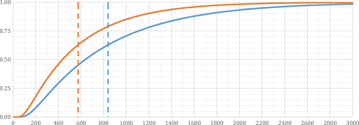
Figure 7: Cdfs and means for the randomised consensus model ($H=6,K=4$)

We have implemented the three new unfolding-free algorithms within mcsta, the Modest Toolset’s stochastic timed systems model checker. When asked to compute $\mathrm{P}^{\mathrm{R}[\leq{n}]}_{\!{\mathit{opt}}}({\cdot})$, it also delivers all values $\mathrm{P}^{\mathrm{R}[\leq{i}]}_{\!{\mathit{opt}}}({\cdot})$ for $i\in\{\,0,\dots,n\,\}$ since the algorithms allow doing so at no overhead. Instead of a single value, we thus get the entire (sub-)cdf. Every single value is defined via an individual optimisation over schedulers. However, we have seen in Sect. 3.4 that an optimal scheduler for bound $i$ can be extended to an optimal scheduler for $i+1$, so there exists an optimal scheduler for all bounds. The max./min. cdf represents the probability distribution induced by that scheduler. We show these functions for the randomised consensus case study [17] in Fig. 7. The top curve is the max. probability for the protocol to terminate within the number of coin tosses given on the x-axis. The bottom curve is the min. probability. For comparison, we also show the means $\mathrm{R}_{\!{\mathrm{min}}}({\cdot})$ and $\mathrm{R}_{\!{\mathrm{max}}}({\cdot})$ of these distributions as the left and right dashed lines, respectively. Note that the min. expected value corresponds to the max. bounded probabilities and vice-versa. As mentioned, using our new algorithms, it is now possible to compute the curves in the same amount of memory (and, in this case, also runtime) previously sufficient for the means only.

We also implemented a convergence criterion to detect when the result will no longer increase for higher bounds. Recall that UnboundedVI terminates when the max. error in the last iteration is below $\epsilon$ (default $\epsilon=10^{-6}$). Our implementation considers the max. error $e$ over all iterations of a call to UnboundedVI in modvi or StepBoundedVI in senum and elim. In the same spirit as the unbounded value iteration algorithm, we can then stop when $e<\epsilon$. For the functions shown in Fig. 7, this happens at 4016 coin tosses for the max. and 5607 for the min. probability.

5 Experiments

Table 4: State spaces

			unfolded		non-unfolded				eliminated
model		$b$	states	time	states	trans	branch	time	states	trans	branch
BEB	4	58	114 k	2 s	2 k	3 k	4 k	0 s	1 k	1 k	3 k
	5	90	803 k	6 s	10 k	12 k	22 k	0 s	3 k	5 k	19 k
	6	143	5.9 M	35 s	45 k	60 k	118 k	0 s	16 k	28 k	104 k
	7	229	44.7 M	273 s	206 k	304 k	638 k	1 s	80 k	149 k	568 k
	8	371	$>\!30\text{\scriptsize\,min}$		1.0 M	1.6 M	3.4 M	3 s	0.4 M	0.8 M	3.1 M
	9	600			4.6 M	8.3 M	18.9 M	26 s	2.0 M	4.2 M	16.6 M
	10	n/a			22.2 M	44.0 M	102.8 M	138 s	$>\!16\text{\scriptsize\,GB}$
BRP	32, 06, 2	179	9.4 M	40 s	0.1 M	0.1 M	0.1 M	0 s	0.1 M	0.4 M	7.1 M
	32, 06, 4	347	50.2 M	206 s	0.2 M	0.2 M	0.2 M	1 s	0.2 M	1.0 M	20.3 M
	32, 12, 2	179	21.8 M	90 s	0.2 M	0.2 M	0.3 M	1 s	0.2 M	1.1 M	22.1 M
	32, 12, 4	347	122.0 M	499 s	0.6 M	0.7 M	0.7 M	2 s	0.6 M	3.2 M	62.0 M
	64, 06, 2	322	38.2 M	157 s	0.1 M	0.2 M	0.2 M	0 s	0.1 M	1.3 M	53.8 M
	64, 06, 4	630	206.9 M	826 s	0.4 M	0.4 M	0.5 M	1 s	0.4 M	3.8 M	153.7 M
	64, 12, 2	322	107.0 M	427 s	0.5 M	0.5 M	0.5 M	1 s	0.4 M	4.1 M	166.0 M
	64, 12, 4	630	$>\!30\text{\scriptsize\,min}$		1.3 M	1.4 M	1.5 M	4 s	$>\!16\text{\scriptsize\,GB}$
RCONS	4, 4	2653	53.9 M	365 s	41 k	113 k	164 k	0 s	35 k	254 k	506 k
	4, 8	7793	$>\!30\text{\scriptsize\,min}$		80 k	220 k	323 k	0 s	68 k	499 k	997 k
	6, 2	2175			1.2 M	5.0 M	7.2 M	5 s	1.1 M	23.6 M	47.1 M
	6, 4	5607			2.3 M	9.4 M	13.9 M	9 s	2.2 M	42.2 M	84.3 M
CSMA	1	2941	31.2 M	276 s	13 k	13 k	13 k	0 s	13 k	13 k	15 k
	2	3695	191.1 M	1097 s	96 k	96 k	97 k	0 s	95 k	95 k	110 k
	3	5229	$>\!30\text{\scriptsize\,min}$		548 k	548 k	551 k	2 s	545 k	545 k	637 k
	4	8219			2.7 M	2.7 M	2.7 M	9 s	2.7 M	2.7 M	3.2 M
FW	short	2487	8.8 M	150 s	4 k	6 k	6 k	0 s	4 k	111 k	413 k
	long	3081	$>\!30\text{\scriptsize\,min}$		0.2 M	0.5 M	0.5 M	1 s	0.2 M	2.4 M	7.7 M

Table 5: Performance

modvi

senum

elim

model

$b$

iter

#

mem

rate

enum

mem

elim

iter

mem

rate

BEB

4

58

0 s

257

40 M

$\infty\text{\scriptsize\,$\frac{\text{1}}{\text{s}}$}$

0 s

41 M

0 s

0 s

40 M

$\infty\text{\scriptsize\,$\frac{\text{1}}{\text{s}}$}$

5

90

0 s

407

40 M

850 $\frac{\text{1}}{\text{s}}$

0 s

45 M

0 s

0 s

48 M

$\infty\text{\scriptsize\,$\frac{\text{1}}{\text{s}}$}$

6

143

1 s

651

54 M

223 $\frac{\text{1}}{\text{s}}$

1 s

65 M

0 s

0 s

107 M

1430 $\frac{\text{1}}{\text{s}}$

7

229

6 s

1055

127 M

38 $\frac{\text{1}}{\text{s}}$

11 s

210 M

2 s

0 s

409 M

1145 $\frac{\text{1}}{\text{s}}$

8

371

49 s

1714

345 M

7 $\frac{\text{1}}{\text{s}}$

88 s

588 M

12 s

2 s

1.5 G

247 $\frac{\text{1}}{\text{s}}$

9

600

425 s

2769

1.7 G

1 $\frac{\text{1}}{\text{s}}$

960 s

2.6 G

67 s

14 s

6.6 G

43 $\frac{\text{1}}{\text{s}}$

10

n/a

$>\!30\text{\scriptsize\,min}$

$>\!30\text{\scriptsize\,min}$

$>\!16\text{\scriptsize\,GB}$

BRP

32, 06, 2

179

1 s

803

55 M

256 $\frac{\text{1}}{\text{s}}$

160 s

474 M

4 s

1 s

775 M

164 $\frac{\text{1}}{\text{s}}$

32, 06, 4

347

4 s

1419

85 M

102 $\frac{\text{1}}{\text{s}}$

498 s

1.2 G

12 s

7 s

2.6 G

61 $\frac{\text{1}}{\text{s}}$

32, 12, 2

179

3 s

803

90 M

85 $\frac{\text{1}}{\text{s}}$

569 s

1.3 G

13 s

4 s

2.8 G

56 $\frac{\text{1}}{\text{s}}$

32, 12, 4

347

13 s

1419

196 M

33 $\frac{\text{1}}{\text{s}}$

1467 s

3.5 G

40 s

22 s

6.1 G

20 $\frac{\text{1}}{\text{s}}$

64, 06, 2

322

3 s

1414

76 M

129 $\frac{\text{1}}{\text{s}}$

$>\!30\text{\scriptsize\,min}$

31 s

16 s

4.7 G

24 $\frac{\text{1}}{\text{s}}$

64, 06, 4

630

17 s

2605

137 M

45 $\frac{\text{1}}{\text{s}}$

114 s

91 s

14.1 G

8 $\frac{\text{1}}{\text{s}}$

64, 12, 2

322

10 s

1414

146 M

40 $\frac{\text{1}}{\text{s}}$

132 s

51 s

13.9 G

8 $\frac{\text{1}}{\text{s}}$

64, 12, 4

630

50 s

2605

318 M

15 $\frac{\text{1}}{\text{s}}$

$>\!16\text{\scriptsize\,GB}$

RCONS

4, 4

2653

37 s

21728

62 M

124 $\frac{\text{1}}{\text{s}}$

2 s

126 M

1 s

3 s

224 M

1842 $\frac{\text{1}}{\text{s}}$

4, 8

7793

222 s

66704

85 M

65 $\frac{\text{1}}{\text{s}}$

4 s

187 M

2 s

16 s

384 M

933 $\frac{\text{1}}{\text{s}}$

6, 2

2175

1383 s

19136

679 M

2 $\frac{\text{1}}{\text{s}}$

$>\!30\text{\scriptsize\,min}$

136 s

169 s

11.9 G

20 $\frac{\text{1}}{\text{s}}$

6, 4

5607

$>\!30\text{\scriptsize\,min}$

275 s

879 s

13.4 G

11 $\frac{\text{1}}{\text{s}}$

CSMA

1

2941

4 s

11904

45 M

1548 $\frac{\text{1}}{\text{s}}$

5 s

46 M

0 s

0 s

60 M

$\infty\text{\scriptsize\,$\frac{\text{1}}{\text{s}}$}$

2

3695

23 s

15061

66 M

312 $\frac{\text{1}}{\text{s}}$

$>\!30\text{\scriptsize\,min}$

1 s

3 s

190 M

2437 $\frac{\text{1}}{\text{s}}$

3

5229

170 s

21426

185 M

62 $\frac{\text{1}}{\text{s}}$

3 s

24 s

839 M

429 $\frac{\text{1}}{\text{s}}$

4

8219

1270 s

33538

606 M

13 $\frac{\text{1}}{\text{s}}$

19 s

192 s

3.8 G

86 $\frac{\text{1}}{\text{s}}$

FW

short

2487

1 s

6012

40 M

2072 $\frac{\text{1}}{\text{s}}$

29 s

79 M

0 s

1 s

113 M

3109 $\frac{\text{1}}{\text{s}}$

long

3081

51 s

9431

107 M

60 $\frac{\text{1}}{\text{s}}$

205 s

880 M

13 s

23 s

1.4 G

132 $\frac{\text{1}}{\text{s}}$

We use five case studies from the literature to evaluate the applicability and performance of our three algorithms and their implementation:

• BEB [8]: MDP of a bounded exponential backoff procedure with max. backoff value $K=4$ and $H\in\{\,4,\dots,10\,\}$ parallel hosts. We compute the max. probability of any host seizing the line while all hosts enter backoff $\leq b$ times.

• BRP [10]: The PTA model of the bounded retransmission protocol with $N\in\{\,32,64\,\}$ frames to transmit, retransmission bound $\mathit{MAX}\in\{\,6,12\,\}$ and transmission delay $\mathit{TD}\in\{\,2,4\,\}$ time units. We compute the max. and min. probability that the sender reports success in $\leq b$ time units.

• RCONS [17]: The randomised consensus shared coin protocol MDP as described in Sect. 4 for $N\in\{\,4,6\,\}$ parallel processes and constant $K\in\{\,2,4,8\,\}$.

• CSMA [10]: PTA model of a communication protocol using CSMA/CD, with max. backoff counter $\mathit{BCMAX}\in\{\,1,\dots,4\,\}$. We compute the min. and max. probability that both stations deliver their packets by deadline $b$ time units.

• FW [17]: PTA model (“Impl” variant) of the IEEE 1394 FireWire root contention protocol with either a short or a long cable. We ask for the min. probability that a leader (root) is selected before time bound $b$.

Experiments were performed on an Intel Core i5-6600T system (2.7 GHz, 4 cores) with 16 GB of memory running 64-bit Windows 10 and a timeout of 30 minutes.

If we look back at the description of the algorithms in Sect. 3, we see that the only extra states introduced by modvi compared to checking an unbounded probabilistic reachability or expected-reward property are the new states $s_{\mathrm{new}}$. However, this can be avoided in the implementation by checking for reward-one branches on-the-fly. The transformations performed in senum and elim, on the other hand, will reduce the number of states, but may add transitions and branches. elim may also create large intermediate models. In contrast to modvi, these two algorithms may thus run out of memory even if unbounded properties can be checked. In Table 4, we show the state-space sizes (1) for the traditional unfolding approach (“unfolded”) for the bound $b$ where the values have converged, (2) when unbounded properties are checked or modvi is used (“non-unfolded”), and (3) after state elimination and merging in elim. We report thousands (k) or millions (M) of states, transitions (“trans”) and branches (“branch”). The values for senum are the same as for elim. Times are for the state-space exploration phase only, so the time for “non-unfolded” will be incurred by all three new algorithms. We see that avoiding unfolding is a drastic reduction. In fact, 16 GB of memory are not sufficient for the larger unfolded models, so we had to enable mcsta’s disk-based technique [12]. State elimination leads to an increase in transitions and especially branches, drastically so for BRP, the exception being BEB.

In Table 5, we report the performance results for all three new algorithms when run until the values have converged at bound value $b$. For senum, we used the variant based on value iteration since it consistently performed better than the one using DTMC state elimination. “iter” denotes the time needed for (unbounded or step-bounded) value iteration, while “enum” and “elim” are the times needed for scheduler enumeration resp. state elimination and merging. “#” is the total number of outer-loop iterations performed during the calls to UnboundedVI. “rate” is the number of bound values computed per second. Memory usage in columns “mem” is mcsta’s peak working set, including state space exploration, reported in mega- (M) or gigabytes (G). mcsta is garbage-collected, so these values are higher than necessary since full collections only occur when the system runs low on memory. The values related to value iteration for senum are the same as for elim. In general, we see that senum uses less memory than elim, but is much slower in all cases. If it works and does not blow up the model too much, elim is significantly faster than modvi, making up for the time spent on state elimination with much faster value iteration rates.

6 Conclusion

We presented three algorithms to model-check cost-/reward-bounded properties on MDP without unfolding. In contrast to recent related work similar to our first algorithm [3, 13], we also consider the application to time-bounded properties on PTA.By avoiding unfolding and returning the entire probability distribution at no extra cost, our techniques could finally make cost-bounded probabilistic (timed) model checking feasible in practical applications.

Outlook.

The digital clocks approach for PTA was considered the most limited in scalability. Our techniques lift some of its most significant practical limitations. Moreover, time-bounded analysis without unfolding and with computation of the entire distribution in this manner is not feasible for the traditionally more scalable zone-based approaches [20] because zones abstract from concrete timing. We see the possibility to improve the state elimination approach by removing transitions that are linear combinations of others and thus unnecessary. This may reduce the transition and branch blowup on models like the BRP case.

Our algorithms senum and elim can be extended to long-run average properties. For a random variable $X_{i}$ for the reward obtained in each step, their value is defined as (A) $\mathcal{E}^{\mathfrak{S}}_{M}(\lim_{n\to\infty}({\sum_{i=0}^{n}X_{i}^{\prime}})/({n+1}))$. This allows to express e.g. the average energy usage or the expected amount of time spent in some system state. Note this is only appropriate if one transition corresponds to one abstract time unit, which is not the case in a digital clocks MDP. In practice, also long-run reward-average properties are of interest, e.g. average energy consumption per subtask performed. They can be expressed by using a second reward variable $Y_{i}$ and considering (B) $\mathcal{E}^{\mathfrak{S}}_{M}(\lim_{n\to\infty}({\sum_{i=0}^{n}X_{i}})/({\sum_{i=0}^{n}Y_{i}}))$. Previous work on solving (B) uses graph decomposition and linear programming [1, 6, 7]. Using the ideas of senum and elim, we can transform this problem into (A), for which the policy iteration-based algorithm of Howard and Veinott [15, 21, 22] is applicable.

References

- [1] de Alfaro, L.: How to specify and verify the long-run average behavior of probabilistic systems. In: LICS. pp. 454–465. IEEE Computer Society (1998)
- [2] Andova, S., Hermanns, H., Katoen, J.: Discrete-time rewards model-checked. In: FORMATS. LNCS, vol. 2791, pp. 88–104. Springer (2003)
- [3] Baier, C., de Alfaro, L., Forejt, V., Kwiatkowska, M.: Probabilistic Model Checking. Springer (2016), to appear.
- [4] Baier, C., Katoen, J.P.: Principles of Model Checking. MIT Press (2008)
- [5] Berendsen, J., Chen, T., Jansen, D.N.: Undecidability of cost-bounded reachability in priced probabilistic timed automata. In: TAMC. LNCS, vol. 5532, pp. 128–137. Springer (2009)
- [6] Bianco, A., de Alfaro, L.: Model checking of probabilistic and nondeterministic systems. In: FSTTCS. LNCS, vol. 1026, pp. 499–513. Springer (1995)
- [7] von Essen, C., Jobstmann, B.: Synthesizing systems with optimal average-case behavior for ratio objectives. In: iWIGP. EPTCS, vol. 50, pp. 17–32 (2011)
- [8] Giro, S., D’Argenio, P.R., Ferrer Fioriti, L.M.: Partial order reduction for probabilistic systems: A revision for distributed schedulers. In: CONCUR. LNCS, vol. 5710, pp. 338–353. Springer (2009)
- [9] Hahn, E.M., Hermanns, H., Zhang, L.: Probabilistic reachability for parametric Markov models. STTT 13(1), 3–19 (2011)
- [10] Hartmanns, A., Hermanns, H.: A Modest approach to checking probabilistic timed automata. In: QEST. pp. 187–196. IEEE Computer Society (2009)
- [11] Hartmanns, A., Hermanns, H.: The Modest Toolset: An integrated environment for quantitative modelling and verification. In: TACAS. LNCS, vol. 8413, pp. 593–598. Springer (2014)
- [12] Hartmanns, A., Hermanns, H.: Explicit model checking of very large MDP using partitioning and secondary storage. In: ATVA. LNCS, vol. 9364, pp. 131–147. Springer (2015)
- [13] Hashemi, V., Hermanns, H., Song, L.: Reward-bounded reachability probability for uncertain weighted MDPs. In: VMCAI. LNCS, vol. 9583. Springer (2016)
- [14] Hatefi, H., Braitling, B., Wimmer, R., Ferrer Fioriti, L.M., Hermanns, H., Becker, B.: Cost vs. time in stochastic games and Markov automata. In: SETTA. LNCS, vol. 9409, pp. 19–34. Springer (2015)
- [15] Howard, R.A.: Dynamic Programming and Markov Processes. John Wiley & Sons Inc., New York (1960)
- [16] Kwiatkowska, M.Z., Norman, G., Parker, D.: PRISM 4.0: Verification of probabilistic real-time systems. In: CAV. LNCS, vol. 6806, pp. 585–591. Springer (2011)
- [17] Kwiatkowska, M.Z., Norman, G., Parker, D.: The PRISM benchmark suite. In: QEST. pp. 203–204. IEEE Computer Society (2012)
- [18] Kwiatkowska, M.Z., Norman, G., Parker, D., Sproston, J.: Performance analysis of probabilistic timed automata using digital clocks. Formal Methods in System Design 29(1), 33–78 (2006)
- [19] Kwiatkowska, M.Z., Norman, G., Segala, R., Sproston, J.: Automatic verification of real-time systems with discrete probability distributions pp. 101–150
- [20] Norman, G., Parker, D., Sproston, J.: Model checking for probabilistic timed automata. Formal Methods in System Design 43(2), 164–190 (2013)
- [21] Puterman, M.L.: Markov Decision Processes: Discrete Stochastic Dynamic Programming. John Wiley & Sons Inc., New York (1994)
- [22] Veinott, A.F.: On finding optimal policies in discrete dynamic programming with no discounting. Annals of Mathematical Statistics 37(5), 1284–1294 (1966)