Spectra of heavy-light mesons in a relativistic model

Abstract

The spectra and wave functions of heavy-light mesons are calculated within a relativistic quark model, which is based on a heavy-quark expansion of the instantaneous Bethe-Salpeter equation by applying the Foldy-Wouthuysen transformation. The kernel we choose is the standard combination of linear scalar and Coulombic vector. The effective Hamiltonian for heavy-light quark-antiquark system is calculated up to order $1/m_{Q}^{2}$. Our results are in good agreement with available experimental data except for the anomalous $D_{s0}^{*}(2317)$ and $D_{s1}(2460)$ states. The newly observed heavy-light meson states can be accommodated successfully in the relativistic quark model with their assignments presented. The $D_{sJ}^{*}(2860)$ can be interpreted as the $|1^{3/2}D_{1}\rangle$ and $|1^{5/2}D_{3}\rangle$ states being members of the 1D family with $J^{P}=1^{-}$ and $3^{-}$.

I Introduction

Great experimental progress has been achieved in studying the spectroscopy of heavy-light mesons in the last decades D2010 ; LHCb ; Ds2632 ; Ds2860 ; Ds2700 ; Ds2009 ; LHCbspin13b ; LHCbspin13a . In the charm sector, several new excited charmed meson states were discovered in addition to the low-lying states. For $D_{J}$ mesons, the excited resonances $D(2740)^{0}$, $D^{*}(2760)$ D2010 , $D_{J}(2580)^{0}$, $D^{*}(2650)$ and $D^{*}(3000)$ LHCb were found in the $D^{(*)}\pi$ invariant mass spectrum by the BaBar and LHCb Collaborations. While for $D_{sJ}$ mesons, besides the well-established $1S$ and $1P$ charmed-strange states, the excited resonances $D_{sJ}(2632)$ Ds2632 , $D_{sJ}(2860)$ Ds2860 , $D_{sJ}(2700)$ Ds2700 and $D_{sJ}(3040)$ Ds2009 were observed in the $D^{(*)}K$ invariant mass distribution by the two collaborations. In the b-flavored meson sector, several excited states were studied in experiment as well as the ground $B$ and $B_{s}$ meson states PDG . The strangeless resonances $B_{J}(5840)^{0}$ and $B(5970)^{0}$ were found in the $B\pi$ invariant mass spectrum by the LHCb and CDF Collaborations, respectively LHCba ; CDFa . While the stranged $B^{*}_{sJ}(5850)$ were observed in the $B^{(*)}K$ invariant mass distribution by the OPAL Collaboration OPAL .

The heavy-light meson spectroscopy plays an important role in understanding the strong interactions between quark and antiquark. In the meanwhile it provides a powerful test of the various phenomenological quark models inspired by QCD. Heavy-light mesons have been investigated extensively in relativistic quark models GI ; cnp ; cccn ; cnp1 ; cflns ; ymz ; GMS , where many relativistic potential models are constructed by modifying or relativizing nonrelativistic quark potential models and additional phenomenological parameters are employed. For heavy-light system, one needs a model that can retain the relativistic effects of the light quark. In this work we resort to the originally relativistic Bethe-Salpeter equation BS . The Bethe-Salpeter approach were widely used in studying mesons so as to embody the relativistic dynamics LS1 ; LS2 ; FK1 ; FK2 ; WWFJ ; CCh . While it is rather difficult to solve the Bethe-Salpeter equation for meson states, especially when considering states with large angular momentum quantum number. In order to study the spectra of heavy-light mesons systematically, we choose to reduce the Bethe-Salpeter equation in the first place.

In our previous work ly3 , we apply the instantaneous approximation and obtain an equation equivalent to the Bethe-Salpeter equation. The Hamiltonian for heavy-light quark-antiquark system is expanded to order $1/m_{Q}$ by applying Foldy-Wouthuysen transformation to the equivalent equation. We find that the leading Hamiltonian is actually not Dirac-like. The interaction we derive is essentially different from the Breit interaction MKM ; TM ; MM . In this paper we extend and improve our study on the spectra of the heavy-light mesons $D$, $D_{s}$, $B$ and $B_{s}$. The running of the coupling constant is considered. Moreover, the $1/m_{Q}^{2}$ correction is calculated. Many papers only considered the leading $1/m_{Q}$ term in the heavy-quark expansion ly3 ; PE ; JZ ; DJ ; DHJ . Our calculation shows that the $1/m_{Q}^{2}$ corrections to the masses of the mesons are around 50 MeV, which is too large to be neglected. The parameters in the equations are determined by fitting the masses of the $1S$ and $1P$ meson states presented by Particle Data Group (PDG) PDG , while the states beyond $1P$ are calculated as a prediction. We find that in the Bethe-Salpeter formalism the linear confining parameter, i.e. the string tension, actually depend on the masses of the constituent quark and antiquark in mesons. The large discrepancy between experimental data and our previous work is decreased in this work. The newly observed heavy-light meson states can be accommodated successfully in our predicted spectra.

This paper is organized as follows. In the next section, we have a brief review of the relativistic quark model. Section III is for the solution of the wave equation and the peturbative corrections. In Section IV, we have numerical results and discussions. The last section is for a brief summary.

II The model

According to the conventional constituent-quark model, the mesons can be seen as a composition of a quark and an antiquark. In the Bethe-Salpeter formalism, the eigenequation for quark-antiquark systems has the general form BS :

$$(p\!\!\!/_{1}-m_{1})\chi(p_{1},p_{2})(p\!\!\!/_{2}+m_{2})$$

$$=\frac{1}{(2\pi)^{4}}\int\!d^{4}p^{\prime}_{1}d^{4}p^{\prime}_{2}\overline{K}(p_{1},p_{2};p^{\prime}_{1},p^{\prime}_{2})\chi(p^{\prime}_{1},p^{\prime}_{2}),$$ (1)

where $p_{1}$ and $p_{2}$ relate to the total momentum $P$ and the relative momentum $p$ as follows:

$$p_{1} = \alpha_{1}P-p,\;\;\alpha_{1}=\frac{m_{1}}{m_{1}+m_{2}},$$ (2)

$$p_{2} = \alpha_{2}P+p,\;\;\alpha_{2}=\frac{m_{2}}{m_{1}+m_{2}}.$$ (3)

Using the energy-momentum conservation, i.e. $p^{\prime}_{1}+p^{\prime}_{2}=p_{1}+p_{2}$, the Eq.(1) can be simplified as:

$$(p\!\!\!/_{1}-m_{1})\chi(p,P)(p\!\!\!/_{2}+m_{2})=\int\!\frac{d^{4}p^{\prime}}{(2\pi)^{4}}\overline{K}(p,p^{\prime},P)\chi(p^{\prime},P).$$ (4)

Here we choose the interaction kernel as the standard Coulomb-plus-linear form, which is one-gluon-exchange (OGE) dominant at short distances with linear confinement at long distances. If one applies the instantaneous approximation, i.e. neglecting the frequency dependence, the kernel can be written as:

$$\overline{K}(p,p^{\prime},P)=\gamma^{(1)}\cdot\gamma^{(2)}V_{v}(-\boldsymbol{k}^{2})+V_{s}(-\boldsymbol{k}^{2}),$$ (5)

where the transferred momentum $\boldsymbol{k}$ is defined as:

$$\boldsymbol{k}=\boldsymbol{p}-\boldsymbol{p}^{\prime}.$$ (6)

Since the interaction kernel $\overline{K}(\boldsymbol{p},\boldsymbol{p}^{\prime},P)$ is no longer dependent on $p^{\prime 0}$, we can perform the integration over $p^{\prime 0}$ in Eq. (4). After transforming the instantaneous Bethe-Salpeter equation into coordinate space, the wave function of the eigenequation decouples from time coordinate GR ; CCW ; CC .

In our previous work ly3 , with the help of projection operators for the wave function we find that the instantaneous Bethe-Salpeter equation is equivalent to the following equation:

$$\left(\omega_{1}+\omega_{2}+\frac{1}{2}(h_{1}+h_{2})U(\boldsymbol{r})\frac{1}{2}(h_{1}+h_{2})-h_{1}E\right)\phi(\boldsymbol{r})=0,$$ (7)

where the superscript “1” and “2” stand for the heavy quark $Q$ and the light antiquark $\bar{q}$ in the $Q\bar{q}$ meson, respectively. The operators in the above equation are defined as:

$$\omega_{i}(\boldsymbol{p}) = \sqrt{\boldsymbol{p}^{2}+m_{i}^{2}},\;\;i=1,2$$ (8)

$$h_{i}(\boldsymbol{p}) = \frac{H_{i}(\boldsymbol{p})}{\omega_{i}(\boldsymbol{p})},\;\;i=1,2$$ (9)

with the free Dirac Hamiltonians

$$H_{1}(\boldsymbol{p}) = {\beta}^{(1)}m_{1}-{\boldsymbol{\alpha}}^{(1)}\cdot\boldsymbol{p},$$ (10)

$$H_{2}(\boldsymbol{p}) = {\beta}^{(2)}m_{2}+{\boldsymbol{\alpha}}^{(2)}\cdot\boldsymbol{p}.$$ (11)

Inserting Eqs. (10) and (11) into Eq.(9), we can verify the relation:

$$h_{i}^{2}(\boldsymbol{p})=1,\;\;i=1,2.\\$$ (12)

The interaction potential $U(\boldsymbol{r})$ in Eq. (7) is directly derived from the instantaneous Bethe-Salpeter equation and closely related to the interaction form we assumed in the kernel. It can be written as:

$$U(\boldsymbol{r})=U_{1}(\boldsymbol{r})+U_{2}(\boldsymbol{r})$$ (13)

with

$$U_{1}(\boldsymbol{r}) = \beta^{(1)}\beta^{(2)}V_{s}(r)+V_{v}(r),$$ (14)

$$U_{2}(\boldsymbol{r}) = -\frac{1}{2}[\,{\boldsymbol{\alpha}}^{(1)}\cdot{\boldsymbol{\alpha}}^{(2)}+({\boldsymbol{\alpha}}^{(1)}\cdot\hat{\boldsymbol{r}})({\boldsymbol{\alpha}}^{(2)}\cdot\hat{\boldsymbol{r}})\,]V_{v}(r),$$

where $V(r)$ and $V(-\boldsymbol{k}^{2})$ are related to each other according to Fourier transformation.

The instantaneous Bethe-Salpeter equation as an integral equation now is equivalent to a less complicated differential equation shown in Eq. (7), but still it is difficult to solve. For heavy-light systems, the heavy quark effective theory is applied. It is reasonable to consider the heavy-quark expansion, i.e. the $1/m_{Q}$ expansion. One can reduce the equivalent eigenequation by calculating the interactions of the heavy-light quark-antiquark meson order by order.

Our goal can be achieved by employing the Foldy-Wouthuysen transformation bGR . The operators involved in Eq. (7) can be divided into two sets: the “odd” $\mathcal{O}$ and the “even” $\mathcal{E}$. The name “odd” denotes that the operators couple the large and small components of the Dirac spinor, while the “even” operators are diagonal with respect to the large and small components. The main idea of the Foldy-Wouthuysen transformation is to apply a unitary transformation $U$ which retains the “even” operators and eliminates the “odd” operators. If one writes the original Hamiltonian as:

$$H=\beta\,m+\mathcal{E}+\mathcal{O},$$ (16)

according to Foldy and Wouthuysen, one obtains the transformed Hamiltonian:

$$\tilde{H} = U^{-1}H\,U$$ (17)

$$= \beta m+\mathcal{E}+\frac{\beta}{2m}\mathcal{O}^{2}+\frac{1}{8m^{2}}[\,[\mathcal{O},\,\mathcal{E}],\,\mathcal{O}\,]+\cdots$$

The reduction by performing the Foldy-Wouthuysen transformation on Eq. (7) is detailed in our previous work ly3 . Instead of $\beta m$ being the main term in the common Dirac Hamiltonian shown in Eq. (16), the dominant term is $\beta E$ in our case:

$$-h_{1}E = \frac{{\boldsymbol{\alpha}}^{(1)}\cdot\boldsymbol{p}-{\beta}^{(1)}m_{1}}{\omega_{1}}E$$

$$= -\beta^{(1)}E+\frac{\boldsymbol{\alpha}^{(1)}\cdot\boldsymbol{p}}{\omega_{1}}E-\beta^{(1)}\left(\frac{m_{1}}{\omega_{1}}-1\right)E.$$

The reduction result is calculated to order $1/m_{Q}$ in our previous work ly3 . With the similar procedure, here we extend the result to order $1/m_{Q}^{2}$. By inserting the “odd” and “even” operators of Eq. (7) into Eq. (17), we obtain the Hamiltonian expansion. After the Foldy-Wouthuysen transformation, we have:

$$\tilde{H} = \tilde{H}_{0}+\tilde{H}^{\prime}$$ (19)

with

$$\tilde{H}_{0} = \omega_{1}+\omega_{2}+\frac{1}{2}\left(1+h_{2}\right)U_{1}\frac{1}{2}\left(1+h_{2}\right),$$ (20)

the perturbative term $\tilde{H}^{\prime}$ consists of various terms of order $1/m_{Q}$ and $1/m^{2}_{Q}$, we divide it into three parts:

$$\tilde{H}^{\prime}=\tilde{H}_{1}^{\prime}+\tilde{H}_{a}^{\prime}+\tilde{H}_{b}^{\prime},$$ (21)

where

$$\tilde{H}_{1}^{\prime} = \frac{1}{2}\left(1+h_{2}\right)\{-\frac{{\boldsymbol{\alpha}}^{(1)}\cdot\boldsymbol{p}}{2m_{1}},\;U_{2}\}\frac{1}{2}\left(1+h_{2}\right),$$ (22)

$$\tilde{H}_{a}^{\prime} = \frac{1}{2}\left(1+h_{2}\right)\frac{{\boldsymbol{\alpha}}^{(1)}\cdot\boldsymbol{p}}{2m_{1}}U_{1}\frac{{\boldsymbol{\alpha}}^{(1)}\cdot\boldsymbol{p}}{2m_{1}}\frac{1}{2}\left(1+h_{2}\right)$$ (23)

$$- \frac{1}{2}\left(-3+h_{2}\right)\frac{{\boldsymbol{p}}^{2}}{8m_{1}^{2}}U_{1}\frac{1}{2}\left(1+h_{2}\right)+h.c.,$$

$$\tilde{H}_{b}^{\prime} = \frac{1}{2}\left(1+h_{2}\right)U_{2}\frac{1}{2}(1+\beta^{(1)}h_{2})U_{1}\frac{{\boldsymbol{\alpha}}^{(1)}\cdot\boldsymbol{p}}{4Em_{1}}+h.c.$$ (24)

$$+ \frac{1}{2}\left(1+h_{2}\right)U_{2}\frac{1}{2}(\beta^{(1)}+h_{2})\frac{{\boldsymbol{\alpha}}^{(1)}\cdot\boldsymbol{p}}{4Em_{1}}U_{1}\frac{1}{2}\left(1+h_{2}\right)$$

$$+ h.c.$$

We can simplify the above equations by inserting an identity matrix $(\gamma^{(1)}_{5})^{2}=1$ between two odd operators of the heavy quark, with the help of the relations $\{\gamma_{5},\;\beta\}=0$, $[\gamma_{5},\;\boldsymbol{\alpha}]=0$, $\gamma_{5}\boldsymbol{\alpha}=\boldsymbol{\Sigma}$ and the substitutions $\beta^{(1)}\rightarrow 1$, $\boldsymbol{\Sigma}^{(1)}\rightarrow\boldsymbol{\sigma}^{(1)}$. Moreover, we can take the substitution $h_{2}\rightarrow 1$ if $h_{2}$ appears at the ends of the expression of $\tilde{H}^{\prime}$ as in Eqs. (22$\sim$24), since the corrections of $\tilde{H}^{\prime}$ are calculated as a perturbation to $\tilde{H}_{0}^{\prime}$.

With the considerations above, we obtain our final Hamiltonian

$$H = H_{0}+H^{\prime},$$ (25)

where the leading order Hamiltonian $H_{0}$ has the form

$$H_{0} = \omega_{1}+\omega_{2}+\frac{1}{2}\left(1+h_{2}\right)\overline{U}_{1}\frac{1}{2}\left(1+h_{2}\right),$$ (26)

and the subleading Hamiltonian $H^{\prime}$ to order $1/m^{2}_{Q}$ can be written as:

$$H^{\prime}=H_{1}^{\prime}+H_{a}^{\prime}+H_{b}^{\prime},$$ (27)

with

$$H_{1}^{\prime} = -\frac{1}{2}\{\frac{{\boldsymbol{\sigma}}^{(1)}\cdot\boldsymbol{p}}{m_{1}},\;\widetilde{U}_{2}\},$$ (28)

$$H_{a}^{\prime} = \frac{1}{4}\frac{{\boldsymbol{\sigma}}^{(1)}\cdot\boldsymbol{p}}{m_{1}}\widetilde{U}_{1}\frac{{\boldsymbol{\sigma}}^{(1)}\cdot\boldsymbol{p}}{m_{1}}+\frac{1}{8}\{\frac{{\boldsymbol{p}}^{2}}{m_{1}},\;\overline{U}_{1}\},$$ (29)

$$H_{b}^{\prime} = \frac{1}{4E}\left(\widetilde{U}_{2}\frac{1}{2}(1-h_{2})\widetilde{U}_{1}\frac{{\boldsymbol{\sigma}}^{(1)}\cdot\boldsymbol{p}}{m_{1}}+h.c.\right)$$ (30)

$$- \frac{1}{4E}\left(\widetilde{U}_{2}\frac{1}{2}(1-h_{2})\frac{{\boldsymbol{\sigma}}^{(1)}\cdot\boldsymbol{p}}{m_{1}}\overline{U}_{1}+h.c.\right),$$

the interaction potentials $\overline{U}_{1}(\boldsymbol{r})$, $\widetilde{U}_{1}(\boldsymbol{r})$ and $\widetilde{U}_{2}(\boldsymbol{r})$ in the above equations are defined as:

$$\overline{U}_{1}(\boldsymbol{r}) = V_{v}(r)+\beta^{(2)}V_{s}(r),$$ (31)

$$\widetilde{U}_{1}(\boldsymbol{r}) = V_{v}(r)-\beta^{(2)}V_{s}(r),$$ (32)

$$\widetilde{U}_{2}(\boldsymbol{r}) = -\frac{1}{2}[{\boldsymbol{\sigma}}^{(1)}\cdot{\boldsymbol{\alpha}}^{(2)}+({\boldsymbol{\sigma}}^{(1)}\cdot\hat{\boldsymbol{r}})({\boldsymbol{\alpha}}^{(2)}\cdot\hat{\boldsymbol{r}})]V_{v}(r).$$

The leading order Hamiltonian $H_{0}$ we obtain for heavy-light quark-antiquark system in Eq. (26) is not Dirac-like as in Refs. JZ ; EFG . Its form is more like the form used in relativized quark models GI ; LY1 ; LY2 . As for double-heavy system, we have $h_{2}\rightarrow 1$ and $\beta^{(2)}\rightarrow 1$, then Eq. (26) can be reduced to:

$$H_{0}^{\rm{Schr}}=\omega_{1}+\omega_{2}+V_{v}(r)+V_{s}(r),$$ (34)

which is the Schrödinger formalism extensively used in nonrelativistic or semirelativistic quark models.

III Solution of the Wave Equation

In this section, we solve the eigenequation of the leading order Hamiltonian $H_{0}$ in Eq. (26). Before doing this, we would like to discuss the properties of the solution of the eigenequation associated with $H_{0}$.

The eigenequation of $H_{0}$ can be written as:

$$\left(\omega_{1}+\omega_{2}+\frac{1}{2}\left(1+h_{2}\right)\overline{U}_{1}\frac{1}{2}\left(1+h_{2}\right)-E\right)\psi=0,$$ (35)

the above equation is equivalent to:

$$h_{2}\left(\omega_{1}+\omega_{2}+\frac{1}{2}\left(1+h_{2}\right)\overline{U}_{1}\frac{1}{2}\left(1+h_{2}\right)-E\right)\psi=0,$$ (36)

which is equivalent to:

$$\left(\omega_{1}+\omega_{2}+\frac{1}{2}\left(1+h_{2}\right)\overline{U}_{1}\frac{1}{2}\left(1+h_{2}\right)-E\right)h_{2}\psi=0.$$ (37)

From Eqs. (35) and (37), we have:

$$h_{2}\psi=c\psi,$$ (38)

and since $(h_{2})^{2}=1$,

$$c=\pm 1.$$ (39)

When we take $c=-1$, Eq. (35) is transformed to:

$$(\omega_{1}+\omega_{2}-E)\psi=0,$$ (40)

which is not the correct eigenequation for bound systems we are interested in. Thus we have only $c=+1$. This is the reason for the substitution $h_{2}\rightarrow 1$ we use in the last section.

While if all the eigenfunctions of $H_{0}$ for bound states satisfy the relation

$$h_{2}\psi=\psi,$$ (41)

the eigenfunction set of $H_{0}$ is NOT complete.

An complete set is needed to construct the identity operator $1=\sum_{i}|\psi_{i}><\psi_{i}|$ in order to calculate the perturbative correction of $H_{b}^{\prime}$, thus we construct a new Hamiltonian. Inspired by the relation $h_{2}\psi=\psi$, we transform the potential term in Eq.(35) as:

$$\frac{1}{2}\left(1+h_{2}\right)\overline{U}_{1}\frac{1}{2}\left(1+h_{2}\right)$$

$$=\frac{1}{4}(\overline{U}_{1}+h_{2}\overline{U}_{1}+\overline{U}_{1}h_{2}+h_{2}\overline{U}_{1}h_{2})$$

$$\Rightarrow\frac{1}{4}(\overline{U}_{1}h_{2}+h_{2}\overline{U}_{1}+\overline{U}_{1}h_{2}+h_{2}\overline{U}_{1})$$

$$=\frac{1}{2}\{h_{2},\;\overline{U}_{1}\},$$

then the new Hamiltonian we construct can be written as:

$$H_{0}=\omega_{1}+\omega_{2}+\frac{1}{2}\{h_{2},\;\overline{U}_{1}\}.$$ (42)

It is easy to verify that the eigenfunction set of the new Hamiltonian includes both subsets:

$$h_{2}\psi^{+}=\psi^{+}\;{\rm and}\;h_{2}\psi^{-}=-\psi^{-},$$ (43)

where the subset $\{\psi^{+}\}$ is identical to the eigenfunction set associated with the original Hamiltonian $H_{0}$ in Eq. (35).

Now we turn to solve the eigenequation associated with the new Hamiltonian $H_{0}$, that is:

$$\left(\omega_{1}+\omega_{2}+\frac{1}{2}\{h_{2},\;\overline{U}_{1}\}-E\right)\psi(\boldsymbol{r})=0.$$ (44)

In the heavy-light quark-antiquark system, we treat the heavy quark as a static source, while the light one is described relativistically by a Dirac spinor. It is easy to verify that $H_{0}$ commute with all the elements of the standard operator set $\{{\boldsymbol{j}}^{2},j_{z},K,S_{z}\}$ associated with the free Dirac Hamiltonian. Then the eigenstates of $H_{0}$ can be labeled by the quantum number set $\{n,j,m_{j},k,s\}$ corresponding to the operator set.

The quantum number $k$ can have two opposite values for a eigenstate with quantum number $j$:

$$k=\pm(j+1/2),\;{\rm for}\;\;l=j\pm 1/2.$$ (45)

The leading order invariant mass $E^{(0)}$ can be determined by quantum numbers $n$, $j$ and $k$, or equivalently by $n$, $j$ and $l$. The parity of the bound states is determined by $P=(-1)^{l+1}$.

The Dirac spinor with quantum numbers $j$ $m_{j}$ and $l$ can be written as:

$$\Psi(\boldsymbol{r})=\left(\begin{array}[]{cc}g(r)\;y_{j,l_{A}}^{m_{j}}(\theta,\varphi)\\ if(r)\;y_{j,l_{B}}^{m_{j}}(\theta,\varphi)\end{array}\right),$$ (46)

where the subscripts $l_{A}$ and $l_{B}$ stand for $l$ and $2j-l$, respectively. The complete expression of $y_{j,l}^{m_{j}}(\theta,\varphi)$ can be found in Ref. PE .

For a bound state of a quark and an antiquark, the wave function will effectively vanish when the distance between them is large enough. We designate such large typical distance as $L$, then the heavy quark and light antiquark bounded in the meson can be viewed as restricted in a limited space, $0<r<L$. Thus we can expand the radial functions $f(r)$ and $g(r)$ by spherical Bessel functions associated with the distance $L$:

$$g(r) = \sum_{i=1}^{N}\frac{g_{i}}{N_{i}^{A}}j_{l_{A}}(\frac{a_{i}^{A}r}{L}),$$ (47)

$$f(r) = \sum_{\alpha=1}^{N}\frac{f_{\alpha}}{N_{\alpha}^{B}}j_{l_{B}}(\frac{a_{\alpha}^{B}r}{L}),$$ (48)

where $N_{n}$ and $a_{n}$ are the module and the $n$-th root of the spherical Bessel function $j_{l}(r)$, respectively.

Inserting Eq. (9) and (11) into Eq. (42), we can rewrite $H_{0}$ in the matrix form

$$H_{0} = \left(\begin{array}[]{cc}\omega_{1}+\omega_{2}&\\ &\omega_{1}+\omega_{2}\end{array}\right)$$ (51)

$$+ \frac{1}{2}\left(\begin{array}[]{cc}H_{a}&H_{b}\\ H_{c}&H_{d}\end{array}\right)+h.c.,$$ (54)

where $h.c.$ stands for Hermitian conjugate and the operator elements are:

$$H_{a} = \frac{m_{2}}{\omega_{2}}(V_{v}+V_{s}),$$ (55)

$$H_{b} = \frac{\boldsymbol{\sigma}\cdot\boldsymbol{p}}{\omega_{2}}(V_{v}-V_{s}),$$ (56)

$$H_{c} = \frac{\boldsymbol{\sigma}\cdot\boldsymbol{p}}{\omega_{2}}(V_{v}+V_{s}),$$ (57)

$$H_{d} = \frac{m_{2}}{\omega_{2}}(V_{s}-V_{v}).$$ (58)

According to Eqs. (47) and (48), we can rewrite the eigenequation of $H_{0}$ in the representation of the state basis constructed by spherical Bessel functions. In this representation, the operator $H_{0}$ can be written in its matrix form:

$$H_{0} = \left(\begin{array}[]{cc}<\omega_{1}+\omega_{2}>_{ij}&\\ &<\omega_{1}+\omega_{2}>_{\alpha\beta}\end{array}\right)$$ (61)

$$+ \frac{1}{2}\left(\begin{array}[]{cc}<H_{a}>_{ij}&<H_{b}>_{i\beta}\\ <H_{c}>_{\alpha j}&<H_{d}>_{\alpha\beta}\end{array}\right)+h.c.$$ (64)

The matrix elements of $H_{0}$ in the above equation can be calculated by applying the relation

$$(\boldsymbol{\sigma}\cdot\boldsymbol{p})\;y_{j,l_{\pm}}^{m_{j}}=\pm i\left(\frac{k\pm 1}{r}\pm\frac{d}{dr}\right)\;y_{j,l_{\mp}}^{m_{j}},$$ (65)

$$l_{A}=l_{+},\;l_{B}=l_{-},$$ (66)

and the eigenequation ly3

$$\Omega(p)\;j_{l}(kr)Y_{lm}(\hat{\boldsymbol{r}})=\Omega(k)\;j_{l}(kr)Y_{lm}(\hat{\boldsymbol{r}}),$$ (67)

where $\Omega(p)$ is a pseudo-differential operator function and $\Omega(k)$ is a normal function, $p$ and $k$ stand for the modules of momentum operator $\boldsymbol{p}$ and momentum $\boldsymbol{k}$, respectively.

With the normalization condition, we can obtain the matrix elements of $H_{0}$ easily. For the operators with respect to energy of motion, we have

$$<\omega_{1}(\boldsymbol{p})+\omega_{2}(\boldsymbol{p})>_{ij} = \left[\;\omega_{1}(\frac{a_{i}^{A}}{L})+\omega_{2}(\frac{a_{i}^{A}}{L})\;\right]\delta_{ij},$$

$$<\omega_{1}(\boldsymbol{p})+\omega_{2}(\boldsymbol{p})>_{\alpha\beta} = \left[\;\omega_{1}(\frac{a_{\alpha}^{B}}{L})+\omega_{2}(\frac{a_{\alpha}^{B}}{L})\;\right]\delta_{\alpha\beta}.$$

In order to write down the expressions of the elements associated with the interaction potential in a compact form, here we introduce a symbolic notation:

$$\left<\,\hat{O}\,\right>_{m,l_{A};n,l_{B}}=\int_{0}^{L}dr\,r^{2}\;j_{l_{A}}(\frac{a_{m}^{A}r}{L})\;\hat{O}\;j_{l_{B}}(\frac{a_{n}^{B}r}{L}),$$ (70)

then we have:

$$<H_{a}>_{ij} = \frac{1}{N_{i}^{A}N_{j}^{A}}\frac{m_{2}}{\omega_{2}(\frac{a_{i}^{A}}{L})}<V_{v}+V_{s}>_{i,l_{A};j,l_{A}},$$

$$<H_{b}>_{i\beta} = \frac{1}{N_{i}^{A}N_{\beta}^{B}}\frac{1}{\omega_{2}(\frac{a_{i}^{A}}{L})}$$

$$\times \left<\left(\frac{k-1}{r}-\frac{d}{dr}\right)(V_{v}-V_{s})\right>_{i,l_{A};\beta,l_{B}},$$

$$<H_{c}>_{\alpha j} = \frac{1}{N_{\alpha}^{B}N_{j}^{A}}\frac{1}{\omega_{2}(\frac{a_{\alpha}^{B}}{L})}$$

$$\times \left<\left(\frac{k+1}{r}+\frac{d}{dr}\right)(V_{v}+V_{s})\right>_{\alpha,l_{B};j,l_{A}},$$

$$<H_{d}>_{\alpha\beta} = \frac{1}{N_{\alpha}^{B}N_{\beta}^{B}}\frac{m_{2}}{\omega_{2}(\frac{a_{\alpha}^{B}}{L})}<V_{s}-V_{v}>_{\alpha,l_{B};\beta,l_{B}}.$$

After calculating every element of the Hermitian matrix of $H_{0}$, we diagonalize the Hermitian matrix and obtain eigenvalues and eigenvectors. The eigenvalue of the matrix is the eigenenergy of $H_{0}$, while the eigenvector are associated with the coefficients $g_{i},f_{\alpha}$, which are defined in Eqs. (47) and (48). That is to say, the eigenequation shown in Eq. (44) is solved and the corresponding eigenenergy and eigenfunction are obtained.

Here we turn to discuss the perturbative corrections of $H^{\prime}$ defined in Eq. (27). The perturbative term $H^{\prime}$ does not commute with the standard operators introduced for the free Dirac Hamiltonian, but still it commutes with the total angular momentum operator $\boldsymbol{J}=\boldsymbol{j}+\boldsymbol{S}$ and the parity operator $\mathcal{P}$ of the bound state.

Thus the quantum number set associated with the total Hamiltonian $H=H_{0}+H^{\prime}$ can be denoted by $\{n,J,M_{J},P\}$. By using Clebsch-Gordan coefficients, the total wave function of the heavy-light quark-antiquark bound state can be decomposed as follows:

$$\Psi^{(0)}_{n,k,j;J,M_{J}}(\boldsymbol{r}) = \sum_{m_{j},s}C^{J,M_{J}}_{j,m_{j};1/2,s}$$ (77)

$$\times \left(\begin{array}[]{cc}g_{n,k,j}(r)\;y_{j,l_{A}}^{m_{j}}(\theta,\varphi)\\ if_{n,k,j}(r)\;y_{j,l_{B}}^{m_{j}}(\theta,\varphi)\end{array}\right)\otimes\chi_{s},$$

with which the corrections and mixings caused by $H^{\prime}$ can be calculated perturbatively. The $1/m_{Q}$ and $1/m^{2}_{Q}$ perturbative terms are given in Eqs. (28$\sim$30).

The properties of the eigenfunctions of $H_{0}$ are of great help in calculating the perturbative corrections. We’ve already used $h_{2}\rightarrow 1$ to get rid of $h_{2}$’s at the ends of the perturbative terms. As for the $h_{2}$’s sandwiched in $H_{b}^{\prime}$, $h_{2}\rightarrow\pm 1$ can be applied due to Eq. (43). $H_{b}^{\prime}$ can be rewritten as:

$$H_{b}^{\prime} = \frac{1}{4E}\widetilde{U}_{2}\frac{1}{2}(1-h_{2})\left(\widetilde{U}_{1}\frac{{\boldsymbol{\sigma}}^{(1)}\cdot\boldsymbol{p}}{m_{1}}-\frac{{\boldsymbol{\sigma}}^{(1)}\cdot\boldsymbol{p}}{m_{1}}\overline{U}_{1}\right)$$ (78)

$$+ h.c.$$

Here we define two operators:

$$\hat{A} = \widetilde{U}_{2},$$

$$\hat{B} = \widetilde{U}_{1}({\boldsymbol{\sigma}}^{(1)}\cdot\boldsymbol{p})-({\boldsymbol{\sigma}}^{(1)}\cdot\boldsymbol{p})\overline{U}_{1}.$$

Then we have:

$$H_{b}^{\prime}=\frac{1}{4m_{1}E}\hat{A}\frac{1}{2}(1-h_{2})\hat{B}+h.c.$$ (79)

As discussed at the beginning of this section, the eigenfunction set of $H_{0}$ can be divided into two parts $\{\psi^{+},\,\psi^{-}\}$, where $\psi^{+}$ and $\psi^{-}$ represent the physical and unphysical states, respectively. Inserting the identity operator composed by the complete set of $H_{0}$ in Eq. (79), we obtain:

$$H_{b}^{\prime} = \frac{1}{4m_{1}E}\hat{A}\frac{1}{2}(1-h_{2})\sum_{i}|\psi_{i}><\psi_{i}|\hat{B}+h.c.$$ (80)

$$= \frac{1}{4m_{1}E}\sum_{m}\hat{A}|\psi^{-}_{m}><\psi^{-}_{m}|\hat{B}+h.c.$$

The correction in first order perturbation can be written as:

$$E_{n,l,j,J}=E^{(0)}_{n,l,j}+\delta E^{(1)}_{n,l,j,J}+\delta E^{(2)}_{n,l,j,J},$$ (81)

where

$$\delta E^{(2)}_{n,l,j,J}=\delta E^{(a)}_{n,l,j,J}+\delta E^{(b)}_{n,l,j,J}.$$ (82)

From Eq. (80), the correction of $H_{b}^{\prime}$ for $\psi^{+}_{n}$ can be written as:

$$\delta E^{(b)}_{n,l,j,J} = \frac{1}{2m_{1}E_{n,l,j}^{(0)}}\sum_{m}<\psi^{+}_{n}|\hat{A}|\psi^{-}_{m}><\psi^{-}_{m}|\hat{B}|\psi^{+}_{n}>$$ (83)

$$= \frac{1}{2m_{1}E_{n,l,j}^{(0)}}\sum_{m}A_{nm}B_{mn}.$$

With the eigenfunctions we obtain, the $1/m_{Q}$ and $1/m^{2}_{Q}$ corrections can be calculated. Then the masses of all the different $J^{P}$ states are determined.

IV Numerical results and discussions

The vector and scalar potentials are chosen to have a Coulombic behavior at short distance and a linear confining behavior at long distance, they can be written in a simple form:

$$V_{v}(r) = -\frac{4\alpha_{s}(r)}{3r},$$ (84)

$$V_{s}(r) = b\;r+c.$$ (85)

The running coupling constant $\alpha_{s}(r)$ in the vector potential is derived from the coupling constant $\alpha_{s}(Q^{2})$ in momentum space via Fourier transformation. It can be parametrized in a more convenient form GI :

$$\alpha_{s}(r)=\sum_{i}\alpha_{i}\frac{2}{\sqrt{\pi}}\int_{0}^{\gamma_{i}r}e^{-x^{2}}dx,$$ (86)

where $\alpha_{i}$ and $\gamma_{i}$ are parameters which can be fitted according to the behavior of the running coupling constant at short distance predicted by QCD. The behavior of $\alpha_{s}(r)$ is depicted in Fig. 1. In this work, $\alpha_{1}=0.25$, $\alpha_{2}=0.15$, $\alpha_{3}=0.20$, and $\gamma_{1}=1/2$, $\gamma_{2}=\sqrt{10}/2$, $\gamma_{3}=\sqrt{1000}/2$, the $\alpha_{i}$ and $\gamma_{i}$ parameters have the same values as in Ref. GI .

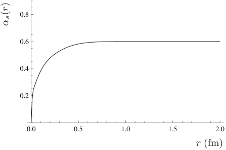
Figure 1: The behavior of the running coupling constant $\alpha_{s}(r)$ with the critical value $\alpha_{s}^{\rm{critical}}=0.6$.

There are two free parameters in the scalar potential. One is the string tensor constant $b$, which characterizes the confinement of the quark-antiquark system. The other is a phenomenological constant $c$, which is adjusted to give the correct ground state energy level of the heavy-light meson state. The behavior of the confinement parameters $b$ in this work is quite different from those in usual quark models. As discussed in our previous paper, the parameter $b$ is responsible for elevating the energy levels of states with higher quantum numbers $n$ or $l$, i.e. the calculated energy gaps between the energy levels of the radial or angular excitations and the ground state depend on the parameter $b$. But unlike the Dirac Hamiltonian:

$$H_{0}^{\rm{Dirac}}=\omega_{1}+H_{2}(\boldsymbol{p})+V_{v}(r)+\beta^{(2)}V_{s}(r),$$ (87)

or the Schrödinger Hamiltonian in Eq. (47), the influence of the confinement potential $V_{s}(r)$ in Eq. (26) weakens as the mass of light quark decreases. That is to say, in the Bethe-Salpeter formalism the energy level is also sensitive to the light quark mass $m_{q}$, which is shown in Fig. 2 by the energy gap $\Delta E$ between the first radial excitation and the ground state as a function of $m_{q}$. We take $B$ meson as an example to illustrate the dependence on the quark mass. The values of the parameters, which are fitted for $B$ meson spectrum, are fixed except for the light quark mass of $B$ meson.

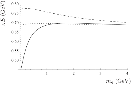
Figure 2: The energy gap $\Delta E$ as a function of the light quark mass in $B$ meson. The dashed, dotted and solid lines stand for the Schrödinger, Dirac and Bethe-Salpeter formalisms, respectively.

From the different shapes of the dashed, dotted and solid lines according to the three schemes, i.e. the Schrödinger, Dirac and Bethe-Salpeter formalisms, one can find:

• When $m_{q}$ is taken large enough, the three schemes tend to give the same value for the energy gap $\Delta E$. It indicates the equivalence of the three schemes when dealing with double-heavy mesons.

• In the region $m_{q}<1{\rm GeV}$, which is the case for heavy-light mesons, the three schemes give quite different values for the energy gap. It has the pattern: $\Delta E^{Schr}>\Delta E^{Dirac}>\Delta E^{B-S}$. In order to give the same energy gap for a specific meson, the confinement parameter should be chosen as: $b^{Schr}<b^{Dirac}<b^{B-S}$. The literature supports this sequence. For instance, $b^{Schr}$ is taken as $0.175\;{\rm GeV}^{2}$ LY2 , $0.180\;{\rm GeV}^{2}$ GI , $b^{Dirac}$ is taken as $0.257\;{\rm GeV}^{2}$ PE , $0.309\;{\rm GeV}^{2}$ MKM , while $b^{B-S}$ can be taken up to $0.400\;{\rm GeV}^{2}$ in this work.

• In the Schrödinger and Dirac schemes, the energy gap changes slowly over $m_{q}$, this is especially true when $m_{q}$ is less then 1 Gev, $\Delta E^{Schr}$ and $\Delta E^{Dirac}$ can be viewed as constants. While in the Bethe-Salpeter scheme, $\Delta E^{B-S}$ changes drastically over $m_{q}$. From the experimental data, we know that the $\Delta E$’s are not sensitive to their light quark masses. For example, the $\Delta E$’s for both $D$ and $D_{s}$ mesons are around $0.7\;{\rm GeV}$. Thus $b^{Schr}$ and $b^{Dirac}$ can be taken as a constant, while $b^{B-S}$ varies with the quark mass.

Our analysis suggests that in the Bethe-Salpeter formalism the string tension $b$ depends on the masses of the quark and antiquark, especially the light one of them.

Besides the potential parameters, four quark mass parameters are employed to fit the heavy-light meson spectra. With all the considerations above, our best fitting of the parameters gives the following values

$$m_{u,d}=0.398\;{\rm GeV},$$

$$m_{s}=0.598\;{\rm GeV},$$

$$m_{c}=1.450\;{\rm GeV},$$

$$m_{b}=4.765\;{\rm GeV},$$

$$b=\left\{\begin{array}[]{llll}0.390\;{\rm GeV}^{2}&{\rm for}\;c\bar{q}\;{\rm system},\\ 0.421\;{\rm GeV}^{2}&{\rm for}\;b\bar{q}\;{\rm system},\\ 0.300\;{\rm GeV}^{2}&{\rm for}\;c\bar{s}\;{\rm system},\\ 0.316\;{\rm GeV}^{2}&{\rm for}\;b\bar{s}\;{\rm system},\end{array}\right.$$ (92)

$$c=-0.320\;{\rm GeV}.$$

In Section III, two numerical parameters $L$ and $N$ are introduced in our calculation. In principle, if the distance $L$ and the size of the expansion basis $N$ are taken to $\infty$, we can obtain the exact solution of the wave equation. Our calculation shows the solution is stable when $L>5$ fm, $N>50$. In this work they are taken as $L=10$ fm, $N=150$, and the size of the matrix of $H_{0}$ in Eq.(64) is $300\times 300$. The Gauss-Legendre quadrature is widely used in our numerical calculation since lots of integrals are involved. After strenuous computation, the meson spectra is obtained. The spectra of the heavy-light $D$, $D_{s}$, $B$, $B_{s}$ mesons are fitted based on the data in PDG PDG . The numerical results for the spectra of $D$, $D_{s}$ mesons are presented in Table 1, while $B$, $B_{s}$ mesons are presented in Table 2. The calculated spectra are in good agreement with the experimental data. Our results are compared to the results of two other relativistic models EFG ; PE , one is derived by quasipotential approach, and the other is obtained by reducing the Bethe-Salpeter vertex function.

The result in this work is improved comparing to our previous work ly3 . Taking the mass difference between the pseudoscalar state and the vector state for example, as shown in Table I, in our previous work, we have:

$$m_{D^{*}}-m_{D} = 167\;{\rm GeV},$$

$$m_{D_{s}^{*}}-m_{D_{s}} = 161\;{\rm GeV},$$

while in this work, we have:

$$m_{D^{*}}-m_{D} = 137\;{\rm GeV},$$

$$m_{D_{s}^{*}}-m_{D_{s}} = 143\;{\rm GeV},$$

the discrepancy from experimental data is decreased for $D$, $D^{*}$, $D_{s}$ and $D_{s}^{*}$ states as well as other states.

Theoretical deviations from experimental data mainly occur in the $D_{s}$ meson sector, specifically, the $D_{s0}^{*}(2317)$ and $D_{s1}(2460)$ resonances. Our calculations for the two resonances are about $100\;{\rm GeV}$ higher than their masses measured in experiment. The discrepancy may be ascribed to the instantaneous approximation, the naive assumption of the kernel or the $\alpha^{2}_{s}(r)$ contributions, i.e. the loop corrections, but it is more likely to be explained beyond naive quark model ws . The masses of the two resonances predicted by constituent quark model are generally $100\sim 200$ MeV higher than experiments JZ ; PE ; GJ ; EGF ; LNR . The mass of $D_{0}^{*}$, $2318\pm 29\;{\rm GeV}$ is almost identical to the mass of $D_{s0}^{*}$, $2317.8\pm 0.6\;{\rm GeV}$. It cannot be explained in conventional quark model if the difference between the two anomalous resonances in the model is merely their light quark masses $m_{s}$ and $m_{u,d}$. In this work the confinement parameter $b$ takes different values for different systems, but still it is not capable to explain the small mass difference of the two resonances.

As the $D_{s0}^{*}$ and $D_{s1}$ lie just below the $DK$ and $D^{*}K$ threshold, respectively, the authors in Ref. BCL have suggested that the two resonance may be $D_{s0}^{*}(DK)$ and $D_{s1}(D^{*}K)$ molecular states, while in Refs. HK1 ; HK2 ; BR , the $D_{s0}^{*}$ and $D_{s1}$ are considered as $c\bar{s}$ states which are significantly affected by mixing with the $DK$ and $D^{*}K$ continua. In Ref. Yu , the authors suggest that the discrepancy of the calculated masses in quark models can be qualitatively understood as a consequence of self-energy effects due to strong coupled channels. In Refs. BEH ; EFR ; EFFR , the interpretation of the heavy $J^{P}(0^{+},1^{+})$ spin multiplet as the parity partner of the groundstate $(0^{-},1^{-})$ multiplet is proposed. Both theoretical and experimental efforts are required in order to fully understand the nature of the anomalous $D_{s0}^{*}(2317)$ and $D_{s1}(2460)$ states.

Besides the well-established $1S$ and $1P$ heavy-light meson states, The highly excited states are also calculated in the spectra and the newly observed highly excited meson states beyond $1P$ are identified in our model.

Table 1: Spectra for $D$ and $D_{s}$ mesons. The comparison of the result in this work with our previous work and other theoretical results in Refs.PE ; EFG is presented. All units are in MeV.

$n^{j}L_{J}$	Meson	$E_{\mathrm{expt.}}$ PDG ; LHCb	$\begin{array}[]{c}\mathrm{this}\\ \mathrm{work}\end{array}$	$\begin{array}[]{c}\mathrm{previous}\\ \mathrm{work}\end{array}$ ​​​​ly3	$\mathrm{Ref.}$ EFG	$\mathrm{Ref.}$ ​ PE
$1^{1/2}S_{0}$	$D$	$1869.62\pm 0.15$	1871	1859	1871	1868
$1^{1/2}S_{1}$	$D^{*}$	$2010.28\pm 0.13$	2008	2026	2010	2005
$1^{1/2}P_{0}$	$D_{0}^{*}(2400)^{0}$	$2318\pm 29$	2364	2357	2406	2377
$1^{1/2}P_{1}$			2507	2529	2469	2490
$1^{3/2}P_{1}$	$D_{1}(2420)$	$2421.3\pm 0.6$	2415	2434	2426	2417
$1^{3/2}P_{2}$	$D_{2}^{*}(2460)$	$2464.4\pm 1.9$	2460	2482	2460	2460
$1^{3/2}D_{1}$			2836	2852	2788	2795
$1^{3/2}D_{2}$			2881	2900	2850	2833
$1^{5/2}D_{2}$	$D_{J}(2740)^{0}$	$2737.0\pm 3.5\pm 11.2$	2737	2728	2806	2775
$1^{5/2}D_{3}$	$D_{J}^{*}(2760)^{0}$	$2760.1\pm 1.1\pm 3.7$	2753	2753	2863	2799
$1^{5/2}F_{2}$			3122	3107	3090	3101
$1^{5/2}F_{3}$			3139	3134	3145	3123
$1^{7/2}F_{3}$	$D^{*}_{J}(3000)^{0}$	$3008.1\pm 4.0$	2980	2942	3129	3074
$2^{1/2}S_{0}$	$D_{J}(2580)^{0}$	$2579.5\pm 3.4\pm 5.5$	2594	2575	2581	2589
$2^{1/2}S_{1}$	$D_{J}^{*}(2650)^{0}$	$2649.2\pm 3.5\pm 3.5$	2672	2686	2632	2692
$2^{1/2}P_{0}$			2895	2902	2919	2949
$2^{1/2}P_{1}$			2983	2999	3021	3045
$2^{3/2}P_{1}$			2926	2932	2932	2995
$2^{3/2}P_{2}$	$D_{J}(3000)^{0}$	$2971.8\pm 8.7$	2965	2969	3012	3035
$2^{3/2}D_{1}$			3230	3228	3228
$2^{3/2}D_{2}$			3259	3260	3307
$2^{5/2}D_{2}$			3159	3139	3259
$2^{5/2}D_{3}$			3176	3160	3335
$2^{5/2}F_{2}$			3455	3425
$2^{5/2}F_{3}$			3465	3444	3551
$2^{7/2}F_{3}$			3346	3301
$1^{1/2}S_{0}$	$D_{s}^{\pm}$	$1968.49\pm 0.32$	1964	1949	1969	1965
$1^{1/2}S_{1}$	$D_{s}^{*\pm}$	$2112.3\pm 0.5$	2107	2110	2111	2113
$1^{1/2}P_{0}$	$D_{s0}^{*}(2317)$	$2317.8\pm 0.6$	2437	2412	2509	2487
$1^{1/2}P_{1}$	$D_{s1}(2536)$	$2535.12\pm 0.13$	2558	2562	2574	2605
$1^{3/2}P_{1}$	$D_{s1}(2460)$	$2459.6\pm 0.6$	2524	2528	2536	2535
$1^{3/2}P_{2}$	$D_{s2}^{*}(2573)$	$2571.9\pm 0.8$	2570	2575	2571	2581
$1^{3/2}D_{1}$	$D_{s1}^{*}(2860)^{-}$	$2859\pm 12\pm 6\pm 23$ LHCbspin13b	2885	2873	2913	2913
$1^{3/2}D_{2}$			2923	2916	2961	2953
$1^{5/2}D_{2}$			2857	2829	2931	2900
$1^{5/2}D_{3}$	$D_{s3}^{*}(2860)^{-}$	$2860.5\pm 2.6\pm 2.5\pm 6.0$ LHCbspin13b	2871	2852	2971	2925
$1^{5/2}F_{2}$			3172	3128	3230	3224
$1^{5/2}F_{3}$			3184	3152	3266	3247
$1^{7/2}F_{3}$			3107	3049	3254	3203
$2^{1/2}S_{0}$	$D_{sJ}(2632)$	$2632.5\pm 1.7$ Ds2632	2647	2624	2688	2700
$2^{1/2}S_{1}$	$D_{s1}^{*}(2710)$	$2708\pm 9^{+11}_{-10}$ Ds2700	2734	2729	2731	2806
$2^{1/2}P_{0}$			2945	2918	3054	3067
$2^{1/2}P_{1}$	$D_{sJ}(3040)$	$3044\pm 8^{+30}_{-5}$ Ds2009	3028	3017	3154	3165
$2^{3/2}P_{1}$			3009	2994	3067	3114
$2^{3/2}P_{2}$			3047	3031	3142	3157
$2^{3/2}D_{1}$			3277	3247	3383
$2^{3/2}D_{2}$			3305	3278	3456
$2^{5/2}D_{2}$			3260	3217	3403
$2^{5/2}D_{3}$			3274	3237	3469
$2^{5/2}F_{2}$			3508	3449
$2^{5/2}F_{3}$			3517	3468	3710
$2^{7/2}F_{3}$			3459	3390

Table 2: Spectra for $B$ and $B_{s}$ mesons. The comparison of the result in this work with our previous work and other theoretical results in Refs.PE ; EFG is presented. All units are in MeV.

$n^{j}L_{J}$	Meson	$E_{\mathrm{expt.}}$ PDG	$\begin{array}[]{c}\mathrm{this}\\ \mathrm{work}\end{array}$	$\begin{array}[]{c}\mathrm{previous}\\ \mathrm{work}\end{array}$ ​​​​ly3	$\mathrm{Ref.}$ EFG	$\mathrm{Ref.}$ ​ PE
$1^{1/2}S_{0}$	$B$	$5279.25\pm 0.17$	5273	5262	5280	5279
$1^{1/2}S_{1}$	$B^{*}$	$5325.2\pm 0.4$	5329	5330	5326	5324
$1^{1/2}P_{0}$			5776	5740	5749	5706
$1^{1/2}P_{1}$			5837	5812	5774	5742
$1^{3/2}P_{1}$	$B_{1}(5721)$	$5723.5\pm 2.0$	5719	5736	5723	5700
$1^{3/2}P_{2}$	$B_{2}^{*}(5747)$	$5743\pm 5$	5739	5754	5741	5714
$1^{3/2}D_{1}$			6143	6128	6119	6025
$1^{3/2}D_{2}$			6165	6147	6121	6037
$1^{5/2}D_{2}$			5993	5989	6103	5985
$1^{5/2}D_{3}$			6004	5998	6091	5993
$1^{5/2}F_{2}$			6379	6344	6412	6264
$1^{5/2}F_{3}$			6391	6354	6420	6271
$1^{7/2}F_{3}$			6202	6175	6391	6220
$2^{1/2}S_{0}$			5957	5915	5890	5886
$2^{1/2}S_{1}$			5997	5959	5906	5920
$2^{1/2}P_{0}$			6270	6211	6221	6163
$2^{1/2}P_{1}$			6301	6249	6281	6194
$2^{3/2}P_{1}$			6216	6189	6209	6175
$2^{3/2}P_{2}$			6232	6200	6260	6188
$2^{3/2}D_{1}$			6514	6458	6534
$2^{3/2}D_{2}$			6527	6471	6554
$2^{5/2}D_{2}$			6401	6357	6528
$2^{5/2}D_{3}$			6411	6365	6542
$2^{5/2}F_{2}$			6692	6621
$2^{5/2}F_{3}$			6700	6629	6786
$2^{7/2}F_{3}$			6553	6493
$1^{1/2}S_{0}$	$B_{s}$	$5366.77\pm 0.24$	5363	5337	5372	5373
$1^{1/2}S_{1}$	$B_{s}^{*}$	$5415.4^{+2.4}_{-2.1}$	5419	5405	5414	5421
$1^{1/2}P_{0}$			5811	5776	5833	5804
$1^{1/2}P_{1}$			5864	5841	5865	5842
$1^{3/2}P_{1}$	$B_{s1}(5830)$	$5829.4\pm 0.7$	5819	5824	5831	5805
$1^{3/2}P_{2}$	$B_{s2}^{*}(5840)$	$5839.7\pm 0.6$	5838	5843	5842	5820
$1^{3/2}D_{1}$			6167	6146	6209	6127
$1^{3/2}D_{2}$			6186	6163	6218	6140
$1^{5/2}D_{2}$			6098	6085	6189	6095
$1^{5/2}D_{3}$			6109	6094	6191	6103
$1^{5/2}F_{2}$			6405	6363	6501	6369
$1^{5/2}F_{3}$			6416	6373	6515	6376
$1^{7/2}F_{3}$			6313	6276	6468	6332
$2^{1/2}S_{0}$			6010	5961	5976	5985
$2^{1/2}S_{1}$			6048	6003	5992	6019
$2^{1/2}P_{0}$			6291	6227	6318	6264
$2^{1/2}P_{1}$			6323	6266	6345	6296
$2^{3/2}P_{1}$			6288	6249	6321	6278
$2^{3/2}P_{2}$			6304	6263	6359	6292
$2^{3/2}D_{1}$			6540	6478	6629
$2^{3/2}D_{2}$			6553	6491	6651
$2^{5/2}D_{2}$			6487	6434	6625
$2^{5/2}D_{3}$			6496	6441	6637
$2^{5/2}F_{2}$			6723	6647
$2^{5/2}F_{3}$			6731	6654	6880
$2^{7/2}F_{3}$			6650	6580

As for $D$ mesons, in the mass region $2500\sim 3000$ MeV several resonances are measured by LHCb collaboration LHCb . The assignments of these states are listed in the upper part of Table I, where the resonances $D_{J}(2740)$, $D_{J}^{*}(2760)$, $D_{J}(3000)$ are identified as $n=1$ states and the resonances $D_{J}(2580)$, $D_{J}^{*}(2650)$, $D_{J}^{*}(3000)$ are identified as radially exited states with $n=2$. In our predicted spectrum for $D$ meson, $D_{J}(2740)$ and $D_{J}^{*}(2760)$ are identified as the $|1^{5/2}D_{2}\rangle$ state with $J=2^{-}$ and the $|1^{5/2}D_{3}\rangle$ state with $J=3^{-}$, respectively. Our best assignment for $D_{J}^{*}(3000)$ is the $|1^{7/2}F_{3}\rangle$ state and $D_{J}(3000)$ the $|2^{3/2}P_{2}\rangle$ state, although in Ref. LHCb they favor the natural and unnatural parity, respectively. The last two resonances $D_{J}(2580)$ and $D_{J}^{*}(2650)$ are identified as the first radial excitations of the ground $D$ and $D^{*}$ states. Recently, LHCb collaboration observed $D_{J}^{*}(2650)$ and $D_{J}^{*}(2760)$, their masses and widths were measured as LHCb2016 :

$$M(D_{1}^{*}(2680)^{0}) = 2681.1\pm 5.6\pm 4.9\pm 13.1\;\mbox{MeV},$$

$$\Gamma(D_{1}^{*}(2680)^{0}) = 186.7\pm 8.5\pm 8.6\pm 8.2\;\mbox{MeV},$$

$$M(D_{3}^{*}(2760)^{0}) = 2775.5\pm 4.5\pm 4.5\pm 4.7\;\mbox{MeV},$$

$$\Gamma(D_{3}^{*}(2760)^{0}) = 95.3\pm 9.6\pm 7.9\pm 33.1\;\mbox{MeV}.$$

From Table 1, one can see our results favor the measurement.

As for $D_{s}$ mesons, several states beyond $1P$ state have been observed, their masses and identifications are presented in the lower part of Table 1. Recently, LHCb collaboration identifies $D_{sJ}^{*}(2860)$ as an admixture of two resonances: $D_{s3}^{*}(2860)^{-}$ and $D_{s1}^{*}(2860)^{-}$ LHCbspin13b ; LHCbspin13a , with their masses measured as $2859\pm 12\pm 6\pm 23\;\mbox{MeV}$ and $2860.5\pm 2.6\pm 2.5\pm 6.0\;\mbox{MeV}$, respectively. In Refs. PE ; EFG cited in Table 1, their predictions do not favor this identification, with their calculations generally 60 MeV higher than the measured masses. While our results for both $|1^{3/2}D_{1}\rangle$ and $|1^{5/2}D_{3}\rangle$ are around 2860 MeV, the two resonances can be interpreted as members of the 1D family with $J^{P}=1^{-}$ and $3^{-}$. The resonances $D_{sJ}(2632)$ , $D_{s1}^{*}(2710)$ and $D_{sJ}(3040)$ are identified as radially exited states with $n=2$ in our model. The $D_{sJ}(2632)$ was firstly observed by SELEX Collaboration at a mass of $2632.5\pm 1.7$ MeV, it can be assigned as the $|2^{1/2}S_{0}\rangle$. The assignment for $D_{s1}^{*}(2710)$ is proposed as $J^{P}=1^{-}$ in Refs. CFNR ; CTLS , which agree with our prediction as our calculated mass for $|2^{1/2}S_{1}\rangle$ is close to its experimental mass $2708\pm 9^{+11}_{-10}$ MeV Ds2700 . The $D_{sJ}(3040)$ resonance is observed in the $D^{*}K$ mass spectrum at a mass of $3044\pm 8_{-5}^{+30}$ MeV by BABAR Collaboration Ds2009 . Here we assign it as $|2^{1/2}P_{1}\rangle$ in our predicted $D_{s}$ meson spectrum.

In the b-flavored meson sector, experimental data for excited $B$ meson states are limited for now. But still several b-flavored mesons are observed CCL . The strangeless resonances $B_{J}(5840)^{0}$ and $B(5970)^{0}$ were measured by the LHCb and CDF Collaborations, respectively LHCba ; CDFa . The stranged $B^{*}_{sJ}(5850)$ were observed by the OPAL Collaboration OPAL . Their masses were measured as:

$$M(B_{J}(5840)) = 5862.9\pm 5.0\pm 6.7\pm 0.2\;\mbox{MeV},$$

$$M(B(5970)^{0}) = 5978\pm 5\pm 12\;\mbox{MeV},$$

$$M(B^{*}_{sJ}(5850)) = 5853\pm 15\;\mbox{MeV}.$$

In table 2, we can identify $B_{J}(5840)^{0}$ and $B(5970)^{0}$ as $|1^{1/2}P_{1}\rangle$ and $|2^{1/2}S_{1}\rangle$, respectively in the spectrum of $B$ meson, while $B^{*}_{sJ}(5850)$ can be assigned as $|1^{1/2}P_{1}\rangle$ in the spectrum of $B_{s}$ meson.

Finally, after solving the wave equation one can obtain not only the eigenenergy of each bound state but also their wave functions. The radial wave functions $g_{n,l,j}(r)$ and $f_{n,l,j}(r)$ for physical and unphysical $D$ meson states are depicted as an example in Fig. 3 and 4, respectively. We stress that the solution of the eigenequation associated with the original $H_{0}$ in Eq. (26) gives only the wavefunctions of physical states depicted in Fig. 3. In Section III we construct a new $H_{0}$ for heavy-light systems in Eq. (42), the unphysical states depicted in Fig. 4 is due to the new $H_{0}$ for which the original one is substituted.

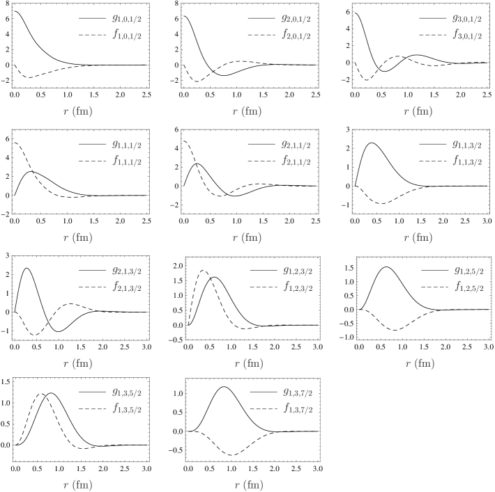
Figure 3: The radial wave functions $g_{n,l,j}(r)$ and $f_{n,l,j}(r)$ for physical $D$ meson states as an example. The wave functions are the radial part of the solution of the eigenequation associated with $H_{0}$.

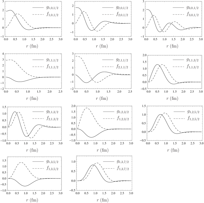
Figure 4: The radial wave functions $g_{n,l,j}(r)$ and $f_{n,l,j}(r)$ for unphysical $D$ meson states as an example. The wave functions are the radial part of the solution of the eigenequation associated with $H_{0}$.

V Summary

The spectra of heavy-light mesons are restudied in a relativistic model, which is derived by reducing the instantaneous Bethe-Salpeter equation. The kernel is chosen to be the standard combination of linear scalar and Coulombic vector. By applying the Foldy-Wouthuysen transformation on the heavy quark, the Hamiltonian for heavy-light quark-antiquark system is calculated up to order $1/m_{Q}^{2}$. We find that in the framework of instantaneous Bethe-Salpeter equation the string tension $b$ in the confinement potential is sensitive to the masses of the constituent quarks in the meson. The spectra of $D$, $D_{s}$, $B$ and $B_{s}$ mesons calculated in the relativistic model. Most of the heavy-light meson states can be accommodated successfully in our model except for the anomalous $D_{s0}^{*}(2317)$ and $D_{s1}(2460)$ resonances. In the Bethe-Salpeter formalism, the assumption of the interaction kernel for mesons is rather a priori, kernels with other spin structures can also be studied. In this work, we only restrict in calculating the spectra of heavy light mesons. With the wave functions obtained when solving the wave equation, $B$ and $D$ decays can be studied in further researches.

References

- (1) P. del Amo Sanchez et al. (BaBar Collaboration), Phys. Rev. D, 82: 111101 (2010)
- (2) R. Aaij et al. (LHCb Collaboration), JHEP 1309: 145 (2013)
- (3) A. V. Evdokimov et al. (SELEX Collaboration), Phys. Rev. Lett. 93: 242001 (2004)
- (4) B. Aubert et al. (BaBar Collaboration), Phys. Rev. Lett. 97: 222001 (2006)
- (5) J. Brodzicka et al. (Belle Collaboration), Phys. Rev. Lett. 100: 092001 (2008)
- (6) B. Aubert et al. (BaBar Collaboration), Phys. Rev. D, 80: 092003 (2009)
- (7) R. Aaij et al. (LHCb Collaboration), Phys. Rev. D, 90: 072003 (2014)
- (8) R. Aaij et al. (LHCb Collaboration), Phys. Rev. Lett. 113: 162001 (2014)
- (9) K. A. Olive et al. (Particle Data Group), Chin. Phys. C, 38: 090001 (2014)
- (10) R. Aaij et al. (LHCb Collaboration), JHEP 04: 024 (2015)
- (11) T. A. Aaltonen et al. (CDF Collaboration), Phys. Rev. D 90: 012013 (2014)
- (12) R. Akers et al. (OPAL Collaboration), Z. Phys. C 66: 19 (1995)
- (13) S. Godfrey and N. Isgur, Phys. Rev. D, 32: 189 (1985)
- (14) P. Cea et al. Phys. Lett. B, 206: 691 (1988)
- (15) P. Cea, G. Nardulli, and G. Paiano, Phys. Rev. D, 28: 2291 (1983)
- (16) P. Colangelo, G. Nardulli, M. Pietroni, Phys. Rev. D, 43: 3002 (1991)
- (17) P. Colangelo et al. Eur. Phys. J. C, 8: 81 (1999)
- (18) M. Z. Yang, Eur. Phys. J. C, 72: 1880 (2012)
- (19) S. Godfrey, K. Moats, and E. S. Swanson, Phys. Rev. D, 94: 054025 (2016)
- (20) H. A. Bethe and E. E. Salpeter, Phys. Rev. 84: 1232 (1951)
- (21) W. Lucha, F. Schöberl, Phys. Rev. D, 93: 096005 (2016)
- (22) W. Lucha, F. Schöberl, Phys. Rev. D, 93: 056006 (2016)
- (23) C. S. Fischera, S. Kubrakb, and R. Williamsc, Eur. Phys. J. A, 51: 10 (2015)
- (24) C. S. Fischera, S. Kubrakb, and R. Williamsc, Eur. Phys. J. A, 50: 126 (2014)
- (25) Z. H. Wang, et al. Phys. Lett. B, 706: 389 (2012)
- (26) C. H. Chang and Y. Q. Chen, Phys. Rev. D, 49: 3399 (1994)
- (27) J. B. Liu and M. Z. Yang, Chinese Physics C, Vol. 40, No. 7 (2016) 073101. arXiv: 1507.08372 [hep-ph].
- (28) J. Morishita, M. Kawaguchi and T. Morii, Phys. Rev. D, 37: 159 (1988)
- (29) T. Matsuki, Mod. Phys. Lett. A, 11: 257 (1996)
- (30) T. Matsuki and T. Morii, Phys. Rev. D, 56: 5646 (1997)
- (31) Y. B. Dai and H. Y. Jin, Phys. Rev. D, 52: 236 (1995)
- (32) Y. B. Dai, C. S. Huang and H. Y. Jin, Phys. Lett. B, 331: 174 (1994)
- (33) J. Zeng, J. W. Van Orden, W. Roberts, Phys. Rev. D, 52: 5229 (1995)
- (34) M. Di Pierro and E. Eichten, Phys. Rev. D, 64: 114004 (2001)
- (35) G. L. Wang, Phys. Lett. B, 633: 492 (2006)
- (36) C. H. Chang, J. K. Chen and G. L. Wang, arXiv: hep-th/0312250
- (37) C. H. Chang and J. K. Chen, Commun. Theor. Phys. 44: 646 (2005)
- (38) W. Greiner and J. Reinhart, Quantum Electrodynamics[M], Springer-Verlag, Berlin, Heidelberg, New York, 2003.
- (39) D. Ebert, R. N. Faustov and V.O. Galkin, Eur. Phys. J. C, 66: 197 (2010)
- (40) J. B. Liu, M. Z. Yang, JHEP 1407: 106 (2014)
- (41) J. B. Liu, M. Z. Yang, Phys. Rev. D, 91: 094004 (2015)
- (42) E. S. Swanson, Phys. Rep. 429: 243 (2006)
- (43) S. Gupta, and J. Johnson, Phys. Rev. D, 51: 168 (1995)
- (44) D. Ebert, V. Galkin, and R. Faustov, Phys. Rev. D, 57 5663 (1998)
- (45) T. Lahde, C. Nyfalt, and D. Riska, Nucl. Phys. A, 674 141 (2000)
- (46) T. Barnes, F. E. Close and H. J. Lipkin, Phys. Rev. D, 68: 054006 (2003)
- (47) D. S. Hwang and D. W. Kim, Phys. Lett. B, 601: 137 (2004)
- (48) D.S. Hwang and D. W. Kim, Phys. Lett. B, 606: 116 (2005)
- (49) E. van Beveren and G. Rupp, Phys. Rev. Lett. 91: 012003 (2003)
- (50) H. Y. Cheng and F. S. Yu, Phys. Rev. D, 89: 114017 (2014)
- (51) W. A. Bardeen, E. J. Eichten and C. T. Hill, Phys. Rev. D, 68: 054024 (2003)
- (52) D. Ebert, T. Feldmann and H. Reinhardt, Phys. Lett. B, 388: 154 (1996)
- (53) D. Ebert, T. Feldmann, R. Friedrich et al. Nucl. Phys. B, 434: 619 (1995)
- (54) P. Colangelo, F. De Fazio, S. Nicotri et al. Phys. Rev. D, 77: 014012 (2008)
- (55) E. F. Close, C. E. Thmas, O. Lakhina et al. Phys. Lett. B, 647: 159 (2007)
- (56) R. Aaij et al. (LHCb Collaboration) Phys. Rev. D, 94 072001 (2016)
- (57) H. X. Chen, W. Chen et al. arXiv:1609.08928 [hep-ph]