Phase transitions in disordered systems: the example of the random-field Ising model in four dimensions

Abstract

By performing a high-statistics simulation of the $D=4$ random-field Ising model at zero temperature for different shapes of the random-field distribution, we show that the model is ruled by a single universality class. We compute to a high accuracy the complete set of critical exponents for this class, including the correction-to-scaling exponent. Our results indicate that in four dimensions: (i) dimensional reduction as predicted by the perturbative renormalization group does not hold and (ii) three independent critical exponents are needed to described the transition.

Introduction — The random-field Ising model (RFIM) Imry and Ma (1975) is maybe the simplest disordered system in Physics Parisi (1994). Applications in hard and soft condensed matter Physics are many (see e.g. Nattermann (1998); Belanger (1998); Fytas and Martín-Mayor (2015)), and their numbers increase Franz et al. (2013); Franz and Parisi (2013); Biroli et al. (2014). The RFIM Hamiltonian is

$${\cal H}=-J\sum_{<xy>}S_{x}S_{y}-\sum_{x}h_{x}S_{x}\;,$$ (1)

with the spins $S_{x}=\pm 1$ occupying the nodes of a hyper-cubic lattice in space dimension $D$ with nearest-neighbor ferromagnetic interactions and $h_{x}$ independent random magnetic fields with zero mean and dispersion $\sigma$.

The Renormalization Group (RG) suggests that $D$ is an all-important variable (no less than temperature $T$) Wilson and Kogut (1974). Indeed, at low temperature $T$ and for small-enough disorder (i.e., $\sigma\ll J$), we encounter the ferromagnetic phase, provided that $D\geq 3$ Imbrie (1984); Bricmont and Kupiainen (1987). A phase transition to a disordered, paramagnetic phase occurs upon increasing $T$ or $\sigma$. Yet, for $D=2$, the tiniest $\sigma>0$ suffices to destroy the ferromagnetic phase Aizenman and Wehr (1990). Furthermore, perturbative RG (PRG) computations, employing the mathematically unorthodox replica trick to restore the translation invariance broken by disorder Edwards and Anderson (1975), tell us that the upper critical dimension is $D_{\mathrm{u}}=6$ Aharony (1978) (Mean Field is quantitatively accurate if $D>D_{\mathrm{u}}$).

The RFIM and branched polymers are unique among disordered systems: a supersymmetry Parisi and Sourlas (1979) makes it possible to analyze the PRG to all orders of perturbation theory Parisi and Sourlas (1981). Supersymmetry predicts dimensional reduction: the RFIM critical behaviour in dimension $D$ would be the same of a non-disordered ferromagnet in dimension $D-2$ Young (1977); Parisi and Sourlas (1979). Yet, see above, the RFIM orders in $D=3$ while the ferromagnet in $D=1$ does not.

The failure of the PRG begs the question: Is there an intermediate dimension $D_{\mathrm{int}}<D_{\mathrm{u}}$ such that the PRG is accurate for $D>D_{\mathrm{int}}$? The issue is obviously relevant to all disordered systems .

Yet, the RFIM is a peculiar disordered system. The relevant RG fixed-point is believed to lie at $T=0$ Villain (1985); Bray and Moore (1985); Fisher (1986). Therefore, in order to describe the critical behavior one needs three independent critical exponents and two correlation functions, namely the connected and disconnected propagators, $C^{\mathrm{(con)}}_{xy}$ and $C^{\mathrm{(dis)}}_{xy}$ . At the critical point and for large $r$ ($r$: distance between $x$ and $y$), they decay as

$$C^{\mathrm{(con)}}_{xy}\!\equiv\!\frac{\partial\overline{\langle S_{x}\rangle}}{\partial h_{y}}\!\sim\!\frac{1}{r^{D-2+\eta}}\,;\ C^{\mathrm{(dis)}}_{xy}\!\equiv\!\overline{\langle S_{x}\rangle\langle S_{y}\rangle}\!\sim\!\frac{1}{r^{D-4+\bar{\eta}}}\,,$$ (2)

where the $\langle\ldots\rangle$ are thermal mean values as computed for a given realization, a sample, of the random fields $\{h_{x}\}$. Over-line refers to the average over the samples. The relationship between the anomalous dimensions $\eta$ and $\bar{\eta}$ is hotly debated, and it is one of our main themes here, as it entails the correct parametrization of the neutron-scattering line-shape Slanič et al. (1999); Ye et al. (2004). Supersymmetry predicts $\eta=\bar{\eta}$.

We also recall phenomenological scaling as an alternative to the PRG Imry and Ma (1975); Villain (1985); Bray and Moore (1985); Fisher (1986). The prediction $\bar{\eta}=2\eta$ by Schwartz and coworkers Schwartz and Soffer (1986); Schwartz et al. (1991); Gofman et al. (1993), although not a consequence of phenomenological scaling, has gained ground thoughout the years. However Tarjus and coworkers Tissier and Tarjus (2011, 2012); Tarjus et al. (2013) have suggested that rare events, neglected in Schwartz and Soffer (1986); Schwartz et al. (1991); Gofman et al. (1993), spontaneously break supersymmetry at the intermediate dimension $D_{\mathrm{int}}\approx 5.1$. For $D>D_{\mathrm{int}}$ replica predictions hold: supersymmetry is valid and $\overline{\eta}=\eta$. For $D<D_{\mathrm{int}}$, instead, there are three independent critical exponents.

Unfortunately, both the perturbative and the phenomenological RG approaches lack predictions allowing for detailed comparisons with experiments. In this context numerical simulations become a crucial tool. This is especially true at $T=0$, where fast polynomial algorithms Anglès d’Auriac et al. (1985); Goldberg and Tarjan (1988) allow us to find exact ground states for a wide range of accessible system sizes $L$. This approach has been used mainly at $D=3$ Ogielski (1986); Anglès d’Auriac and Sourlas (1997); Swift et al. (1997); Sourlas (1999); Hartmann and Nowak (1999); Middleton (2001); Hartmann and Young (2001); Middleton and Fisher (2002); Dukovski and Machta (2003); Wu and Machta (2005, 2006); Fytas and Martín-Mayor (2013); Picco and Sourlas (2014) but also for higher dimensions on a smaller scale Swift et al. (1997); Hartmann (2002); Middleton (2002); Ahrens and Hartmann (2011), although having a strong command over the $D$-dependency of the random-field criticality would be desirable and is the motivation of the current work.

Noteworthy, claims of universality violations for the RFIM at $D\geq 3$ have been quite frequent when comparing different distributions of random fields Anglès d’Auriac and Sourlas (1997); Swift et al. (1997); Sourlas (1999); Hartmann and Nowak (1999). Fortunately, using new techniques of statistical analysis Fytas and Martín-Mayor (2015), it has been possible to show that, at least in $D=3$, these apparent universality violations are merely finite-size corrections to the leading scaling behavior Fytas and Martín-Mayor (2013); Picco and Sourlas (2015). We also note the numerical bound $2\eta-\bar{\eta}\leq 0.0026(10)$ Fytas and Martín-Mayor (2013) which is valid in $D=3$ .

Here, we report the results of large-scale zero-temperature numerical simulations at $D=4$. Our state-of-the-art analysis Fytas and Martín-Mayor (2015, 2013) provides high-accuracy estimates for the critical exponents $\eta$, $\bar{\eta}$, and $\nu$, as well as for other RG-invariants, indicating that dimensional reduction does not hold at this particular dimensionality. A clear case for universality is made by comparing Gaussian-and Poissonian-distributed random fields, but only after taming the strong scaling corrections. Finally, we present overwhelming numerical evidence in favor of $2\eta-\bar{\eta}>0$, indicating that three independent critical exponents are needed to describe the transition and, furthermore, that the intermediate space dimension where supersymmetry gets restored is larger than four.

Simulation details and finite-size scaling — We consider the Hamiltonian (1) on a $D=4$ hyper-cubic lattice with periodic boundary conditions and energy units $J=1$. Our random fields $h_{x}$ follow either a Gaussian $({\mathcal{P}}_{G})$, or a Poissonian $({\mathcal{P}}_{P})$ distribution:

$${\mathcal{P}}_{G}(h,\sigma)={1\over\sqrt{2\pi\sigma^{2}}}e^{-{h^{2}\over 2\sigma^{2}}}\;,\ {\mathcal{P}}_{P}(h,\sigma)={1\over 2|\sigma|}e^{-{|h|\over\sigma}}\;,$$ (3)

where $-\infty<h<\infty$. For both distributions $\sigma$ is our single control parameter.

We simulated lattice sizes from $L=4$ to $L=60$. For each $L$ and $\sigma$ value we computed ground states for $10^{7}$ samples, see the Supplemental Material SM sup . For comparison, 3200 samples of $L=32$ were simulated in Hartmann (2002) and 5000 samples of $L=64$ in  Middleton (2002).

From simulations at a given $\sigma$, we computed $\sigma$-derivatives and extrapolated to neighboring $\sigma$ values by means of a reweighting method Fytas and Martín-Mayor (2015). We computed the second-moment correlation length Amit and Martín-Mayor (2005) for each of the two propagators $C^{\mathrm{(con)}}$ and $C^{\mathrm{(dis)}}$ in Eq. (2), $\xi^{\mathrm{(con)}}$ and $\xi^{\mathrm{(dis)}}$, as well as the corresponding susceptibilities $\chi^{\mathrm{(con)}}$ and $\chi^{\mathrm{(dis)}}$. We also computed the dimensionless Binder ratio $U_{4}=\overline{\langle m^{4}\rangle}/\overline{\langle m^{2}\rangle}^{2}$ and the ratio $U_{22}=\chi^{\mathrm{(dis)}}/[\chi^{\mathrm{(con)}}]^{2}$ that gives a direct access to the difference of the anomalous dimensions $2\eta-\bar{\eta}$. For additional technical details see Ref. Fytas and Martín-Mayor (2015).

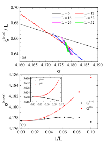
We followed the quotients-method approach to finite-size scaling Amit and Martín-Mayor (2005); Nightingale (1976); Ballesteros et al. (1996). In this method, one considers dimensionless quantities $g(\sigma,L)$ that, barring correction to scaling, are $L$-independent at the critical point. We consider two such $g$, namely $\xi^{\mathrm{(dis)}}/L$ and $\xi^{\mathrm{(con)}}/L$ (also $U_{4}$ is dimensionless). Given a dimensionless quantity $g$, we consider a pair of lattices sizes $L$ and $2L$ and determine the crossing $\sigma_{\mathrm{c},L}$, where $g(\sigma_{\mathrm{c},L},L)=g(\sigma_{\mathrm{c},L},2L)$, see Fig. 1–top. For each random-field distribution we compute two such $\sigma_{\mathrm{c},L}$, one for $\xi^{\mathrm{(dis)}}/L$ and one for $\xi^{\mathrm{(con)}}/L$. Crossings approach the critical point as $\sigma_{\mathrm{c}}-\sigma_{\mathrm{c},L}={\cal O}(L^{-(\omega+1/\nu)})$, with $\omega$ being the leading corrections-to-scaling exponent.

Dimensionful quantities $O$ scale with $\xi$ in the thermodynamic limit as $\xi^{x_{O}/\nu}$, where $x_{O}$ is the scaling dimension of $O$. At finite $L$, we consider the quotient $Q_{O,L}=O_{2L}/O_{L}$ at the crossing (for dimensionless magnitudes $g$, we write $g^{\mathrm{cross}}_{L}$ for either $g_{L}$ or $g_{2L}$, whichever show less finite-size corrections)

$$Q_{O,L}^{\mathrm{cross}}=2^{x_{O}/\nu}+O(L^{-\omega})\;\;;\;\;g^{\mathrm{cross}}_{L}=g^{\ast}+O(L^{-\omega})\,.$$ (4)

$Q_{O}^{\mathrm{cross}}$ (or $g^{\mathrm{cross}}_{L}$) can be evaluated both at the crossing for $\xi^{\mathrm{(dis)}}/L$ or $\xi^{\mathrm{(con)}}/L$. The two choices differ only in the scaling corrections, an opportunity we shall use. The RG tells us that $x_{O}$, $g^{\ast}$, $\omega$, and $\nu$, are universal. We shall compute the critical exponents using Eq. (4) with the following dimensionful quantities: $\sigma$-derivatives [$x_{D_{\sigma}\xi^{\mathrm{(con)}}}=x_{D_{\sigma}\xi^{\mathrm{(dis)}}}=1+\nu$], susceptibilities [$x_{\chi^{\mathrm{(con)}}}=\nu(2-\eta)$ and $x_{\chi^{\mathrm{(dis)}}}=\nu(4-\bar{\eta})$] and the ratio $U_{22}$ [$x_{U_{22}}=\nu(2\eta-\bar{\eta})$]. We also note the ambiguity with $g^{\mathrm{cross}}_{L}$. If you study, say, $g=\xi^{\mathrm{(dis)}}/L$ at the crossings of $\xi^{\mathrm{(con)}}/L$, you may focus just as well on $g_{2L}$, or on $g_{L}$. Scaling corrections can be the smallest in either case. The corrections-minimizing choices are $g^{\mathrm{cross}}_{L}=g_{2L}$ for $\xi^{\mathrm{(dis)}}/L$, $g^{\mathrm{cross}}_{L}=g_{L}$ for $\xi^{\mathrm{(con)}}/L$, and $g^{\mathrm{cross}}_{L}=g_{2L}$ for $U_{4}$.

Now, an important issue is evinced in Fig. 1–bottom: The size evolution is non monotonic (for a spectacular example see Fig. 4–SM sup ). In other words, our accuracy is enough to resolve sub-leading corrections to scaling.

Figure 1: (color online) Top: Connected correlation length in units of the system size $L$ vs. $\sigma$ (we show data only for some characteristic $L$ values for clarity’ sake). Due to scale invariance, all curves should cross at the critical point $\sigma_{\mathrm{c}}$. Yet, small systems deviate from the large-$L$ scale-invariant behavior. Bottom: For Gaussian random fields, crossing points $\sigma_{\mathrm{c},L}$ of pair of lattice-sizes ($L,2L$) for $\xi^{\mathrm{(dis)}}/L$ and $\xi^{\mathrm{(con)}}/L$, as a function of $1/L$. Lines are fits to Eq. (6), constrained to yield a common extrapolation to $L=\infty$ (depicted as a black circle at the origin in this figure and in the following ones). Inset: Same as in bottom panel, but for the case now of Poissonian random fields. In all figures the notation G^(con),(dis) [or P^(con),(dis)] distinguishes the type of crossing point (or the type of random fields, i.e., Gaussian or Poissonian).

We take into account sub-leading corrections in an effective way. Let $X_{L}$ be either $g^{\mathrm{cross}}_{L}$ or the effective scaling dimension $x^{\mathrm{(eff)}}_{O}/\nu=\log Q_{O}^{\mathrm{cross}}(L)/\log 2$, recall Eq. (4). We consider two different fits ($a_{k},b_{k},c_{k},d_{k}$ for $k=1,2$ are scaling amplitudes):
(i) The quadratic fit (QF) which is

$$X_{L} = X^{\ast}+a_{1}L^{-\omega}+a_{2}L^{-2\omega}\;,$$ (5)

$$\sigma_{\mathrm{c},L} = \sigma_{c}+b_{1}L^{-(\omega+\frac{1}{\nu})}+b_{2}L^{-(2\omega+\frac{1}{\nu})}\;.$$ (6)

(ii) However, $\omega$ turns out to be so large, that $L^{-2\omega}$ terms (certainly present) are maybe not the most relevant correction. Hence we consider also the leading + analytic corrections fit [(L+A)F],

$$X_{L} = X^{\ast}+c_{1}L^{-\omega}+c_{2}L^{-(2-\eta)}\;,$$ (7)

$$\sigma_{\mathrm{c},L} = \sigma_{c}+d_{1}L^{-(\omega+\frac{1}{\nu})}+d_{2}L^{-(2-\eta+\frac{1}{\nu})}\;.$$ (8)

The $L^{-(2-\eta)}$ term is due to the non-divergent analytic background. We plug $2-\eta\simeq 1.8$ in the (L+A)F.

Since both fits are well motivated only when $L$ is large enough, we restrict ourselves to data with $L\geq L_{\mathrm{min}}$. To determine an acceptable $L_{\mathrm{min}}$ we employ the standard $\chi^{2}$-test for goodness of fit, where $\chi^{2}$ is computed using the complete covariance matrix. In practice, we found that both types of fit give compatible results. In the following, we present the results of the QF [for the results of the (L+A)F, see Tab. 1].

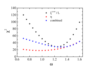
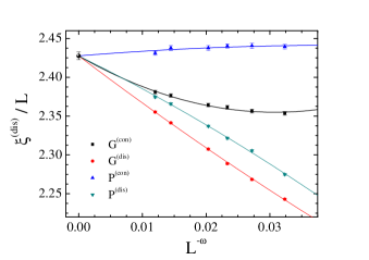
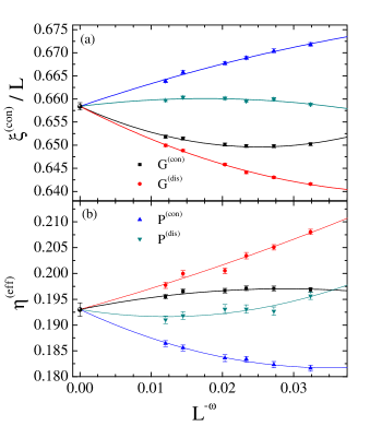
Results — The procedure we follow is standard by now Ballesteros et al. (1998). The first step is the estimation of the corrections-to-scaling exponent $\omega$. Take, for instance, $\xi^{\mathrm{(con)}}/L$. For each pair of sizes $(L,2L)$ we have four estimators, Fig. 2–top: two crossing points, either $\xi^{\mathrm{(con)}}/L$ or $\xi^{\mathrm{(dis)}}/L$, and two disorder distributions. Rather than four independent fits to Eq. (5), we perform a single joint fit: we minimize the combined $\chi^{2}$ goodness-of-fit, by imposing that the extrapolation to $L=\infty$, $(\xi^{\mathrm{(con)}}/L)^{\ast}$, as well as exponent $\omega$ are common for all four estimators (only the scaling amplitudes differ). We judge from the final $\chi^{2}$ value whether or not the fit is fair.

Furthermore, one can perform joint fits for several magnitudes, say $\xi^{\mathrm{(con)}}/L$ and $\eta$. Of course, the extrapolation to $L=\infty$ is different for each magnitude, but a common $\omega$ is imposed. However, when we increase the number of magnitudes, the covariance matrix becomes close to singular due to data correlation, and the fit becomes unstable. Therefore, we limit ourselves to $\xi^{\mathrm{(con)}}/L$ and $\eta$, see Fig. 2 and Fig. 5–SM sup . We obtain a fair fit, Table 1, by considering pairs $(L,2L)$ with $L\geq L_{\mathrm{min}}=14$.

Figure 2: (color online) Top: $\xi^{\mathrm{(con)}}/L$ vs. $L^{-\omega}$ at the crossing points shown in the upper panel of Fig. 1. Bottom: The same as in top panel, but for $\eta^{\mathrm{(eff)}}$. Lines correspond to the joint fit reported in Table 1.

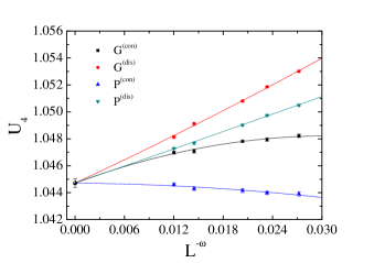
The rest of the quantities of interest are individually extrapolated, following the same procedure, but now fixing $\omega=1.30(9)$ (For the extrapolation of $\xi^{\mathrm{(dis)}}/L$ and $U_{4}$ see Figs. 6–SM and 7–SM in sup ). In fact, the extrapolations in Tab. 1 have two error bars. The first error, obtained from the corresponding joint fit to Eq. (5), is of statistical origin. The second error is systematic and takes into account how much the extrapolation to $L=\infty$ changes in the range $1.21<\omega<1.39$.

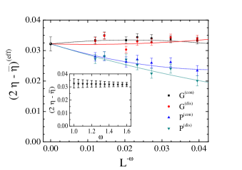
Our main result is illustrated in Fig. 3, where we show $\log U_{22}/\log 2$ which is a direct measurement of the difference $2\eta-\bar{\eta}$. This extrapolation is particularly easy, because $L_{\mathrm{min}}=12$ is enough to obtain a good fit and a value $2\eta-\bar{\eta}=0.0322(24)$. Furthermore, the dependency on $\omega$ of the large-$L$ extrapolation is weak, as shown in Fig. 3–inset. We conclude with high confidence that $2\eta-\bar{\eta}$ is different than zero, in support of the three-exponent scaling scenario.

Figure 3: (color online) Effective anomalous dimension difference $2\eta-\bar{\eta}$ vs. $L^{-\omega}$ at the crossing points shown in the upper panel of Fig. 1. Lines correspond to a joint fit to Eq. (5) with $\omega=1.3$. Inset: The extrapolation to large-$L$ of $2\eta-\bar{\eta}$ is essentially $\omega$-independent.

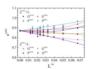
We also determined the effective exponent $\nu^{\mathrm{(eff)}}$ from the $\sigma$-derivatives of $\xi^{\mathrm{(con)}}$ and $\xi^{\mathrm{(dis)}}$ (see Fig. 8–SM sup ). The fits were acceptable even with $L_{\mathrm{min}}=8$ (Table 1).

Previous less accurate numerical estimates for the Gaussian distribution of random fields that did not take into account sub-leading corrections are given by Hartmann: $\nu=0.78(10)$, $\sigma_{\mathrm{c}}=4.18(1)$, $\eta=0.18(1)$, and $\bar{\eta}=0.37(5)$ (so that $2\eta-\bar{\eta}\approx-0.01$) Hartmann (2002) and Middleton: $\nu=0.82(6)$ and $\sigma_{\mathrm{c}}=4.179(2)$ Middleton (2002). We may also quote the functional RG estimates $2\eta-\bar{\eta}=0.08(4)$, $\nu=0.81(3)$ and $\eta=0.24(1)$ Tissier and Tarjus (2012), close but incompatible with our findings, probably due to the truncation of the functional RG equations.

Conclusions — We have carried out a zero-temperature numerical study of the random-field Ising model in four dimensions. By using two types of the random-field distribution and a proper finite-size scaling scheme we have been able to show universality and to determine with high accuracy the three independent critical exponents, $\eta$, $\bar{\eta}$, and $\nu$, that are needed to describe the transition, as well as other renormalization group invariants. We stress the non-trivial difference between the anomalous dimensions $2\eta-\bar{\eta}=0.0322(24)$ which is ten times larger than its corresponding value at $D=3$ Fytas and Martín-Mayor (2013). We thus provided decisive evidence in favor of the three-exponent scaling scenario and the spontaneous supersymmetry breaking Tissier and Tarjus (2011, 2012) at some $D_{\mathrm{int}}>4$, against the (restricted) scaling picture Schwartz and Soffer (1986); Schwartz et al. (1991); Gofman et al. (1993).

Let us conclude by mentioning our preliminary simulations in five dimensions, not reported here. Critical exponents in $D=5$ turn out to be very close to those of the $D=3$ pure Ising ferromagnet, as supersymmetry and dimensional reduction predict. This finding suggests that $D_{\mathrm{int}}\approx 5$, in quantitative agreement with Refs. Tissier and Tarjus (2011, 2012). We intend to pursue this investigation in the near future. As for the suspected upper critical dimension, $D_{\mathrm{u}}=6$, characteristic logarithmic scaling violations have been reported Ahrens and Hartmann (2011), but still await detailed confirmation. These two final steps will give us access to the full picture of the RFIM scaling behavior.

Table 1: Summary of results. The second column is the outcome of a fit to Eq. (5) while the fourth column is obtained fitting to Eq. (7) [yet, critical points $\sigma_{\mathrm{c}}$ were obtained from Eqs. (6) or (8), correspondingly]. The first row reports a joint fit for $\omega$, $\xi^{\mathrm{(con)}}/L$ and $\eta$. The remaining quantities were individually extrapolated to $L=\infty$. $\chi^{2}$ is the standard figure of merit (DOF: number of degrees of freedom in the fit).

	QF	$\chi^{2}/{\mathrm{DOF}}$	(L + A)F	$\chi^{2}/{\mathrm{DOF}}$
$\omega$	1.30(9)		1.60(14)
$\xi^{\mathrm{(con)}}/L$	0.6584(8)	27.85/29	0.6579 (+6/-4)	40.33/37
$\eta$	0.1930(13)		0.1922(10)
$\sigma_{\mathrm{c}}(G)$	4.17749(4)(2)	5.6/7	4.17750(4)(2)	3.2/7
$\sigma_{\mathrm{c}}(P)$	3.62052(3)(8)	8.85/11	3.62060(3)(1)	9.8/11
$U_{4}$	1.04471(32)(14)	10/11	1.04490(36)(9)	8.57/11
$\xi^{\mathrm{(dis)}}/L$	2.4276(36)(34)	16/15	2.4225(41)(20)	14/15
$\nu$	0.8718(58)(19)	62.9/55	0.8688(64)(11)	59.8/55
$2\eta-\bar{\eta}$	0.0322 (23)(1)	16.0/19	0.0322(25)(1)	16.1/19

Supplemental Material

The algorithm used to generate the ground states of the system was the push-relabel algorithm of Tarjan and Goldberg Goldberg and Tarjan (1988). We prepared our own C version of the algorithm, involving a modification proposed by Middleton et al. Middleton (2001); Middleton and Fisher (2002); Middleton (2002) that removes the source and sink nodes, reducing memory usage and also clarifying the physical connection Middleton and Fisher (2002); Middleton (2002). Additionally, the computational efficiency of our algorithm has been increased via the use of periodic global updates Middleton and Fisher (2002); Middleton (2002).

We simulated systems with lattice sizes within the range $L=4-60$. In particular, we considered the sizes $L=\{4,5,6,8,10,12$, $14,16,18,20,24,26,28,30,32,36,40,52,60\}$, so that we created up to $12$ pairs of system sizes $(L,2L)$ in order to apply the quotients method. For each set ($L,\sigma$) and for each field distribution, Gaussian and Poissonian, we simulated $10^{7}$ independent random-field realizations. As we applied the quotients method at both the crossings of the connected and disconnected correlation length over the system size, i.e., $\xi^{\rm(con)}/L$ and $\xi^{\rm(dis)}/L$, typically the sets of simulations were doubled for each system size as the crossings between the connected and disconnected cases varied. Note also, that throughout the main manuscript we have used the notation $\rm{Z}^{\rm(x)}$, where Z denotes the distribution, i.e., G for Gaussian and P for Poissonian, and the superscript x refers to the connected (con) and disconnected (dis) type of the universal ratio $\xi^{\rm(x)}/L$.

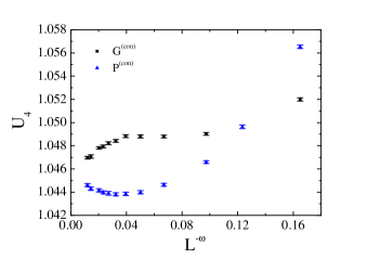
We present in Fig. 4 the result for the Binder cumulant $U_{4}$ for the complete lattice-size spectrum, starting from $L=4$ (compare to Fig. 7 below where results are shown for $L\geq 16$). Results are given for both the Gaussian and Poissonian distributions estimated at the crossings of the $\xi^{\rm(con)}/L$. Although $U_{4}$ converges toward a unique value in the large size limit in support of universality, we observe that by including data for smaller lattices that there is a strong inflection. This justifies our choice of the inclusion of further corrections-to-scaling for smaller system sizes and also consists a clear illustration of misleading behavior at different scaling regimes. We believe that this latter point was behind the strong violations of universality claimed in previous works of the RFIM.

In Fig. 5, we show a complementary plot that supports the claim of Fig. 2 of the main manuscript. In particular, we plot the $\omega$-minimization attempt of the merit of the fit shown Fig. 5, in terms of $\chi^{2}$, for both $\xi^{\rm(con)}/L$ and $\eta$ separately and also for the combined fit that has provided us with the final values of $\xi^{\rm(con)}/L$, $\eta$, as well as the corrections-to-scaling exponent $\omega$.

The extrapolation to the thermodynamic limit of the critical $\xi^{\mathrm{(dis)}}/L$ is illustrated in Fig. 6 (a fair fit was obtained with $L_{\mathrm{min}}=14$). Similarly, also $U_{4}$ converges to its universal limit, as shown in Fig. 7 ($L_{\mathrm{min}}=16$ in this case).

Finally, in Fig. 8 we illustrate the infinite limit-size extrapolation of the effective exponent $\nu$ of the correlation length, for both types of distributions studied. The solid lines are a joint polynomial fit of second order in $L^{-\omega}$ including data points for $L\geq 8$, extrapolating to $L^{-\omega}=0$, as shown by the filled circle in the figure. We remind the reader that for the effective exponent $\nu$ we have two sets of data for each of the two distributions coming from the connected and disconnected correlation lengths.

Figure 4: (color online) $U_{4}$ vs. $L^{-\omega}$ for the complete lattice-size spectrum ($\omega=1.3$).

Figure 5: (color online) Minimum of $\chi^{2}$ as a function of $\omega$ for the fits shown in Fig. 2 of the main manuscript, referring to the universal ratio $\xi^{\rm(con)}/L$, the anomalous dimension $\eta$, and the combined data.

Figure 6: (color online) $\xi^{\mathrm{(dis)}}/L$ vs. $L^{-\omega}$ at the crossing points shown in the upper panel of Fig. 1 in the main text. Lines correspond to a joint fit to Eq. (5) in the main text (with $\omega=1.3$).

Figure 7: (color online) $U_{4}$ vs. $L^{-\omega}$ at the crossing points shown in the upper panel of Fig. 1 in the main text. Lines correspond to a joint fit to Eq. (5) in the main text (with $\omega=1.3$).

Figure 8: (color online) Infinite limit-size extrapolation of the effective critical exponent $\nu$. Lines correspond to a joint fit to Eq. (5) in the main text (with $\omega=1.3$).