Fast and Accurate Performance Analysis
of LTE Radio Access Networks

Abstract

An increasing amount of analytics is performed on data that is procured in a real-time fashion to make real-time decisions. Such tasks include simple reporting on streams to sophisticated model building. However, the practicality of such analyses are impeded in several domains because they are faced with a fundamental trade-off between data collection latency and analysis accuracy.

In this paper, we study this trade-off in the context of a specific domain, Cellular Radio Access Networks (RAN). Our choice of this domain is influenced by its commonalities with several other domains that produce real-time data, our access to a large live dataset, and their real-time nature and dimensionality which makes it a natural fit for a popular analysis technique, machine learning (ML). We find that the latency accuracy trade-off can be resolved using two broad, general techniques: intelligent data grouping and task formulations that leverage domain characteristics. Based on this, we present CellScope, a system that addresses this challenge by applying a domain specific formulation and application of Multi-task Learning (MTL) to RAN performance analysis. It achieves this goal using three techniques: feature engineering to transform raw data into effective features, a PCA inspired similarity metric to group data from geographically nearby base stations sharing performance commonalities, and a hybrid online-offline model for efficient model updates. Our evaluation of CellScope shows that its accuracy improvements over direct application of ML range from 2.5$\times$ to 4.4$\times$ while reducing the model update overhead by up to 4.8$\times$. We have also used CellScope to analyze a live LTE consisting of over 2 million subscribers for a period of over 10 months, where it uncovered several problems and insights, some of them previously unknown.

1 Introduction

Big data analytics have seen tremendous growth in the recent past, with applications in several domains such as social networks, sciences and medicine. Increasingly, the trend in data analytics have moved towards tasks that operate on data that is procured in a real-time fashion and produce low latency decisions. However, such analysis tasks are faced with a fundamental trade-off between latency and accuracy in several domains. In this paper, we consider this trade-off in the context of a domain specific use case: performance diagnostics in cellular Radio Access Networks (RANs). Being the most crucial component in the cellular network architecture, the performance of RANs (in terms of throughput, latency, call drops, etc.) is essential for achieving high quality of experience for end-users. Although RANs work in tandem with the cellular core network to provide service, the lion’s share of user-facing issues in a typical cellular network manifest in the RAN [14]. Thus, to achieve high end-user satisfaction, it is imperative that operators understand the impacting factors and can diagnose RAN problems quickly.

While RAN technologies have seen tremendous improvements over the past decade [40, 34, 36], performance problems are still prevalent [38]. Factors impacting RAN performance include user mobility, skewed traffic pattern, interference, lack of coverage, unoptimized configuration parameters, inefficient algorithms, equipment failures, software bugs and protocol errors [37]. Although some of these factors are present in traditional networks and troubleshooting these networks has received considerable attention in the literature [7, 52, 11, 2, 46], RAN performance diagnosis brings out a unique challenge: the performance of multiple base stations exhibit complex temporal and spatial interdependencies due to the shared radio access media and user mobility.

Existing systems [16, 4] for detecting performance problems rely on monitoring aggregate metrics, such as connection drop rate and throughput per cell, over minutes-long time windows. Degradation of these metrics trigger mostly manual—hence, time-consuming and error-prone—root cause analysis. Furthermore, due to their dependence on aggregate information, these tools either overlook many performance problems such as temporal spikes leading to cascading failures or are unable to isolate root causes. The challenges associated with leveraging just aggregate metrics has led operators to collect detailed traces from their network [15] to aid domain experts in diagnosing RAN problems.

However, the sheer volume of the data and its high dimensionality make the troubleshooting using human experts and traditional rule-based systems very hard, if not infeasible [24]. In this paper, we consider one natural alternative to these approaches that has been used recently to troubleshoot other complex systems with considerable success: machine learning (ML) [30]. However, simply applying ML to our problem is not enough. The desire to troubleshoot RANs as fast as possible exposes the inherent tradeoff between latency and accuracy that is shared by many ML algorithms.

To illustrate this tradeoff, consider the natural solution of building a model on a per-base station basis. On one hand, if we want to troubleshoot quickly, the amount of data collected for a given base station may not be enough to learn an accurate model. On the other hand, if we wait long enough to learn a more accurate model, this will come at the cost of delaying troubleshooting and the learned model may not be valid any longer. Another alternative would be to learn one model over the entire data set. Unfortunately, since base stations can have very different characteristics using a single model for all of them can also result in low accuracy (section 2).

In this paper, we present CellScope, a system that enables fast and accurate RAN performance diagnosis by resolving the latency and accuracy trade-off using two broad techniques: intelligent data grouping and task formulations that leverage domain characteristics. More specifically, CellScope applies Multi-task Learning (MTL) [44, 10], a state-of-the-art machine learning approach, to RAN troubleshooting. In a nutshell, MTL learns multiple related models in parallel by leveraging the commonality between those models. To enable the application of MTL, CellScope uses two techniques. First, it uses feature engineering to identify the relevant features to use for learning. Second, it uses a PCA based similarity metric to group base stations that share common features, such as interference and load. This is necessary since MTL assumes that the models have some commonality which is not necessarily the case in our setting, e.g., different base stations might exhibit different features. Note that while PCA has been traditionally used to find network anomalies, CellScope uses PCA for finding the common features instead. We note that the goal of CellScope is not to apply specific ML algorithms for systems diagnostics, but to propose approaches to resolve the latency accuracy trade-off common in many domains.

To this end, CellScope uses MTL to create a hybrid model: an offline base model that captures common features, and an online per-base station model that captures the individual features of the base stations. This hybrid approach allows us to incrementally update the online model based on the base model. This results in models that are both accurate and fast to update. Finally, in this approach, finding anomalies is equivalent to detecting concept drift [19].

To demonstrate the effectiveness of our proposal, we have built CellScope on Spark [49, 41, 26]. Our evaluation shows that CellScope is able to achieve accuracy improvements upto 4.4$\times$ without incurring the latency overhead associated with normal approaches (section 6). We have also used CellScope to analyze a live LTE network consisting of over 2 million subscribers for a period of over 10 months. Our analysis reveals several interesting insights (section 7).

In summary, we make the following contributions:

• We expose the fundamental trade-off between data collection latency and analysis accuracy present in many domains, which impedes the practicality of applying analytics for decision making on data collected in a real-time fashion. We find that this trade-off may be resolved in several domains using two broad approaches: intelligent grouping and domain specific formulations.

• Based on this insight, we present CellScope, a system that applies a domain specific formulation and application of Multi-task Learning (MTL) to resolve the latency and accuracy trade-off in RAN performance analysis. It achieve this using three techniques: feature engineering to transform raw data into effective features, a novel PCA inspired similarity metric to group data from base stations sharing commonalities in performance, and a hybrid online-offline model for efficient model updates (section 4).

• We have built CellScope on Apache Spark, a big data framework. Our evaluation shows that CellScope’s accuracy improvements range from 2.5$\times$ to 4.4$\times$ while reducing the model update overhead by up to 4.8$\times$ (section 6). We have also validated CellScope by using it to analyze an operational LTE consisting of over 2 million subscribers for a period of over 10 months. Our analysis uncovered insights which were valuable for operators (section 7).

2 Background and Motivation

In this section, we briefly discuss cellular networks, focusing on the LTE network architecture, protocol procedures and measurement data and then motivate the problem.

2.1 LTE Network Primer

LTE networks provide User Equipments (UEs) such as smartphones with Internet connectivity. When a UE has data to send to or receive from the Internet, it sets up a communication channel between itself and the Packet Data Network Gateway (P-GW). This involves message exchanges between the UE and the Mobility Management Entity (MME). In coordination with the base station (eNodeB), the Serving Gateway (S-GW), and P-GW, data plane (GTP) tunnels are established between the base station and the S-GW, and between the S-GW and the P-GW. Together with the connection between the UE and the base station, the network establishes a communication channel called EPS bearer (short for bearer). The entities in the LTE network architecture is shown in figure 1.

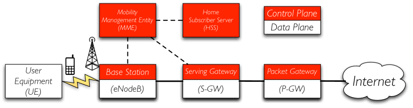
Figure 1: LTE network architecture

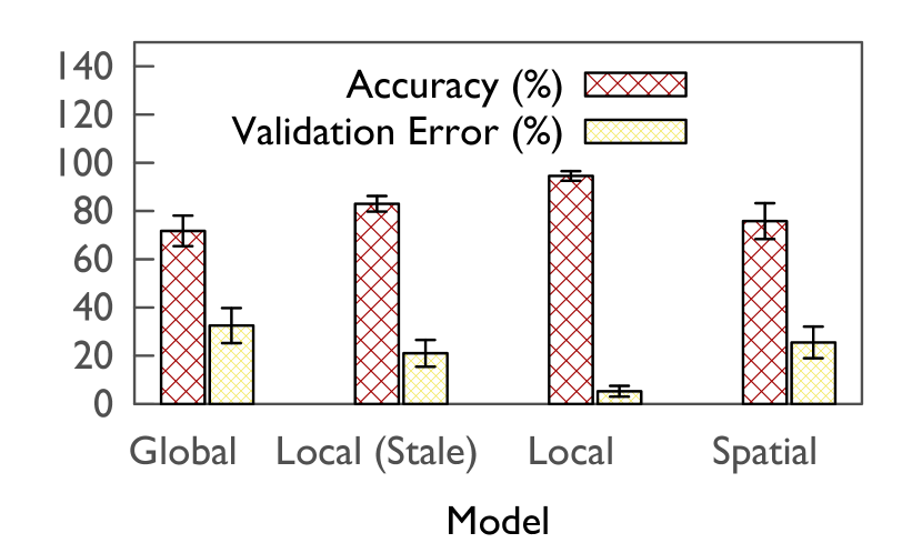
Figure 2: Global models are ineffective while spatial partitioning ignores performance similarity

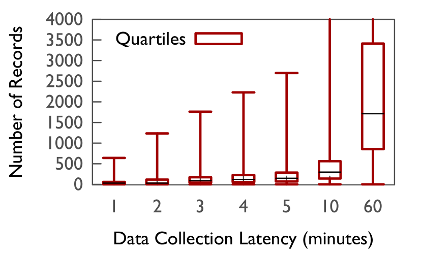
Figure 3: Lack of data at low latencies indicates the need for grouping/partitoning

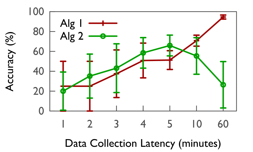
Figure 4: Using local models leads to accuracy and/or latency issues

Figure 5: Resolving the latency accuracy trade-off requires domain specific optimizations.

For network access and service, entities in the LTE network exchange control plane messages. A specific sequence of such control plane message exchange is called a network procedure. For example, when a UE powers up, it initiates an attach procedure with the MME which consists of establishing a radio connection to the base station, authentication and resource allocation. Thus, each network procedure involves the exchange of several control plane messages between two or more entities. The specifications for these are defined by various 3GPP Technical Specification Groups (TSG) [42].

Network performance degrades and end-user experience is affected when procedure failures happen. The complex nature of these procedures (due to the multiple underlying message and entity interactions) make diagnosing problems challenging. Thus, to aid RAN troubleshooting, operators collect extensive measurements from their network. These measurements typically consist of per-procedure information (e.g., attach). To analyze a procedure failure, it is often useful to look at the associated variables. For instance, a failed attachment procedure may be diagnosed if the underlying signal strength information was captured . Hence, relevant metadata is also captured with procedure information. Since there are hundreds of procedures in the network and each procedure can have many possible metadata fields, the collected measurement data contains several hundreds of fields.

2.2 RAN Troubleshooting Today

Current RAN network monitoring depends on cell-level aggregate Key Performance Indicators (KPI). Existing practice is to use performance counters to derive these KPIs. The derived KPIs are then monitored by domain experts, aggregated over certain pre-defined time window. Based on domain knowledge and operational experience, these KPIs are used to determine if service level agreements (SLA) are met. For instance, an operator may have designed the network to have no more than 0.5% call drops in a 10 minute window. When a KPI that is being monitored crosses the threshold, an alarm is raised and a ticket created. This ticket is then handled by experts who investigate the cause of the problem, often manually. Several commercial solutions exists [3, 4, 5, 16] that aid in this troubleshooting procedure by enabling efficient slicing and dicing on data. However, we have learned from domain experts that often it is desirable to apply different models or algorithms on the data for detailed diagnosis. Thus, most of the RAN trouble tickets end up with experts who work directly on the raw measurement data.

2.3 Need for Domain Specific Approach

We now discuss the difficulties in applying machine learning for solving the RAN performance analysis problem, thereby motivating the need for a new domain specific solution.

2.3.1 Ineffectiveness of Global Modelling

A common solution to applying ML on a dataset is to consider the dataset as a single entity and build one model over the entire data. However, base stations in a cellular network exhibit different characteristics. This renders the use of a global model ineffective. To illustrate this problem, we conducted an experiment where the goal was to build a model for call drops in the network. We first run a decision tree algorithm to obtain a single model for the network. The other extreme for this approach is to train a model per base station. Figure 2 shows the results of this experiment which used data collected over an 1 hour interval to ensure there is enough data for the algorithms to produce statistically significant results. We see that the local model is significant better, with up to 20% more accuracy while showing much lower variance.

2.3.2 Latency/Accuracy Issues with Local Models

It is natural to think of a per base station model as the final solution to this problem. However, this approach has issues too. Due to the difference in characteristics of the base stations, the amount of data they collect is different. Thus, in small intervals, they may not generate enough data to produce valid results. This is illustrate in figure 3 which shows the quartiles, min and max amount of data generated and the latency required to collect them.

Additionally, algorithms may produce stale models with increasing latency. To show this, we conduct an experiment with two different algorithms on data collected over varying latencies. The first algorithm (Alg 1) builds a classification model for connection failures, while the second (Alg 2) builds a regression model to predict and explain throughput anomalies. The results of this experiment is given in figure 4. The first algorithm behavior is obvious; as it gets more data its accuracy improves due to the slow varying nature of the underlying causes of failures. After an hour latency, it is able to reach a respectable accuracy. However, the second algorithm’s accuracy improves initially, but falls quickly. This is counterintuitive in normal settings, but the explanation lies in the spatio-temporal characteristics of cellular networks. Many of the performance metrics exhibit high temporal variability, and thus need to be analyzed in smaller intervals. In such cases, local modeling is ineffective.

It is important to note that an obvious, but flawed, conclusion is to think that models similar to Alg 1 would work once the data collection latency has been incurred once. This is not true due to staleness issues which we discuss next.

2.3.3 Need for Model Updates

Due to the temporal variations in cellular networks, models need to be updated to retain their performance. To depict this, we repeated the experiment where we built per base station decision tree model for call drops. However, instead of training and testing on parts of the same dataset, we train on an hours worth of data, and apply it to the next hour. Figure 2 shows that the accuracy drops by 12% with a stale model. Thus, it is important to keep the model fresh by incorporating learning from the incoming data while also removing historical learnings. Such sliding updates to ML models in a general setting is difficult due to the overheads in retraining them from scratch. To add to this, cellular networks consist of several thousands of base stations. This number is on the rise with the increase in user demand and the ease of deployment of small cells. Thus, a per base station approach requires creating, maintaining and updating a huge amount of models (e.g., our network consisted of over 13000 base stations). This makes scaling hard.

2.3.4 Why not Spatial/Spatio-Temporal Partitioning?

The above experiments point towards the need for obtaining enough data with low latency. The obvious solution to combating this trade-off is to intelligently combine data from multiple base stations. It is intuitive to think of this as a spatial partitioning problem, since base stations in the real world are geographically separated. Thus, a spatial partitioner which combines data from base stations within a geographical region must be able to give good results. Unfortunately, this isn’t the case which we motivate using a simple example. Consider two base stations, one situated at the center of times square in New York and the other a mile away at a residential area. Using a spatial partitioning scheme that divides the space into equal sized planes would likely result in combining data from these base stations. However, this is not desirable because of the difference in characteristics of these base stations . We illustrate this using the drop experiment. Figure 2 shows the performance of a spatial model, where we combine data from nearby base stations using a simple grid partitioner. The results show that the spatial partitioner is not much better than the global partitioner. We show comparisons with other smarter spatial partitioning approaches in 6.

3 CellScope Overview

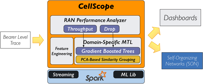
Figure 6: CellScope System Architecture.

CellScope presents a domain-specific formulation and application of Multi-Task Learning (MTL) for RAN performance diagnosis. Here, we provide a brief overview of CellScope to aid the reader in following the rest of this paper.

3.1 Problem Statement

CellScope’s ultimate goal is to enable fast and accurate RAN performance diagnosis by resolving the trade-off between data collection latency and the achieved accuracy. The key difficulty arises from the fundamental trade-off between having not enough data to build accurate-enough models in short timespans and waiting to collect enough data that entails stale results that is impossible to resolve in a general setting. Additionally, we must support efficient modifications to the learned models to account for the temporal nature of our setting to avoid data staleness.

3.2 Architectural Overview

Figure 6 shows the high-level architecture of CellScope, which has the following key components:

Input data: CellScope uses bearer-level traces that are readily available in cellular networks (section 2.1). Base stations collect traces independently and send them to the associated MME. records if required (users move, The MME merges records if required and hence, generate traces at multiple base stations) and uploads them to a data center.

Feature engineering: Next, CellScope uses domain knowledge to transform the raw data and constructs a set of features amenable to learning (e.g., computing interference ratios)(section 4.1). We also leverage protocol details and algorithms (e.g., link adaptation) in the physical layer.

Domain-specific MTL: CellScope uses a domain specific formulation and application of MTL that allows it to perform accurate diagnosis while updating models efficiently (section 4.2).

Data partitioner: To enable correct application of MTL, CellScope implements a partitioner based on a similarity score derived from Principal Component Analysis (PCA) and geographical distance (section 4.3). The partitioner segregates data to be analyzed into independent sets and produces a smaller co-located set relevant to the analysis. This minimizes the need to shuffle data during the training process.

RAN performance analyzer: This component binds everything together to build diagnosis modules. It leverages the MTL component and uses appropriate techniques to build call drop and throughput models. We discuss our experience of applying these techniques to a live LTE network in section 7.

Output: Finally, CellScope can output analytics results to external modules such as RAN performance dashboards. It can also provide inputs to Self-Organizing Networks (SON).

4 Resolving Latency-Accuracy Trade-off

In this section, we present how CellScope uses domain-specific machine learning to mitigate the trade-off between latency and accuracy. We first discuss a high-level overview of RAN specific feature engineering that prepares the data for learning (section 4.1). Next, we describe CellScope’s MTL formulation (section 4.2), discussing how it lets us build fast, accurate, and incremental models. Then, we explain how CellScope achieves grouping that captures commonalities among base stations using a novel PCA based partitioner (section 4.3). Finally, we summarize our approach in section 4.4.

4.1 Feature Engineering

Feature engineering, the process of transforming the raw input data to a set of features that can be effectively utilized by machine learning algorithms, is a fundamental part of ML applications [51]. Generally carried out by domain experts, it is often the first step in applying learning techniques.

Bearer-level traces contain several hundred fields associated with LTE network procedures. Unfortunately, many of these fields are not suitable for model building as it is. Several fields are collected in a format that utilizes a compact representation. For instance, block error rates need to be computed across multiple records to account for time. Further, these records are not self-contained, and multiple records need to be analyzed to create a feature for a certain procedure. In section 7, we describe in detail many of the specific feature engineerings that helped CellScope uncover issues in the network.

4.2 Multi-Task Learning

The latency-accuracy trade-off makes it hard to achieve both low latency and high accuracy in applied machine learning tasks (section 2). The ideal-case scenario in CellScope is if infinite amount of data is available per base station with zero latency. In this scenario, we would have a learning task for each base station that produce a model as an output with the best achievable accuracy. In reality, our setting has several tasks, each with its own data. However, each task does not have enough data to produce models with acceptable accuracy in a given latency budget. This makes our setting an ideal candidate for multi-task learning (MTL), a cutting-edge research area in machine learning. The key idea behind MTL is to learn from other tasks by weakly coupling their parameters so that the statistical efficiency of many tasks can be boosted [10, 44, 17, 9]. Specifically, if we are interested in building a model of the form

$$h(x)=m(f_{1}(x),f_{2}(x),...,f_{k}(x))$$ (1)

where $m$ is a model composed of features $f_{1}$ through $f_{k}$, then the traditional MTL formulation, given dataset $\mathcal{D}=\{(x_{i},y_{i},bs_{i}):i=1,...,n\}$, where $x_{i}\in\mathbb{R}^{d},y_{i}\in\mathbb{R}$ and $bs_{i}$ denotes the $i^{th}$ base station, is to learn

$$h(x)=m_{bs}(f_{1}(x),f_{2}(x),...,f_{k}(x))$$ (2)

where $m_{bs}$ is a per base station model.

In this MTL formulation, the core assumption is a shared structure or dependency across each of the learning problems. Unfortunately, in our setting, the base stations do not share a structure at a global level (section 2). Due to their geographic separation and the complexities of wireless signal propagation, the base stations share a spatio-temporal structure instead. Thus, we proposes a new domain-specific MTL formulation.

4.2.1 CellScope’s MTL Formulation

In order to address the difficulty in applying MTL due to the violation of task dependency assumption in RANs, we can leverage domain-specific characteristics. Although independent learning tasks (learning per base station) are not correlated with each other, they exhibit specific non-random structure. For example, the performance characteristics of base stations nearby are influenced by similar underlying features. Thus, we propose exploiting this knowledge to segregate learning tasks into groups of dependent tasks on which MTL can be applied. MTL in the face of dependency violation has been studied in the machine learning literature in the recent past [25, 20]. However, they assume that each group has its own set of features. This is not entirely true in our setting, where multiple groups may share most or all features but still need to be treated as separate groups. Furthermore, some of the techniques used for automatic grouping without a priori knowledge are computationally intensive.

Assuming we can club learning tasks into groups, we can rewrite the MTL eq. (2) to captures this structure as

$$h(x)=m_{g(bs)}(f_{1}(x),f_{2}(x),...,f_{k}(x))$$ (3)

where $m_{g(bs)}$ is the per-base station model in group $g$. We describe a simple technique to achieve this grouping based on domain knowledge in section 4.3 and experimentally show that just grouping by itself can achieve significant gains in section 6.

In theory, the MTL formulation in eq. (3) should suffice for our purposes as it would perform much better by capturing the inter-task dependencies using grouping. However, this formulation still builds an independent model for each base station. Building and managing a large amount of models leads to significant performance overhead and would impede our goal of scalability. Scalable application of MTL in a general setting is an active area of research in machine learning [31], so we turn to problem-specific optimizations to address this challenge.

The model $m_{g(bs)}$ could be built using any class of learning functions. In this paper, we restrict ourselves to functions of the form $F(x)=w.x$ where $w$ is the weight vector associated with a set of features $x$. This simple class of function gives us tremendous leverage in using standard algorithms that can easily be applied in a distributed setting, thus addressing the scalability issue. In addition to scalable model building, we must also be able to update the built models fast. However, machine learning models are typically hard to update in real time. To address this challenge, we discuss a hybrid approach to building the models in our MTL setting next.

4.2.2 Hybrid Modeling for Fast Model Updates

Estimation of the model in eq. (3) could be posed as an $\ell_{1}$ regularized loss minimization problem [45]:

$$min\sum L(h(x:f_{bs}),y)+\lambda||R(x:f_{bs})||$$ (4)

where $L(h(x:f_{bs}),y)$ is a non-negative loss function composed of parameters for a particular base station, hence capturing the error in the prediction for it in the group, and $\lambda>0$ is a regularization parameter scaling the penalty $R(x:f_{bs})$ for the base station. However, the temporal and streaming nature of the data collected means that the model must be refined frequently for minimizing staleness.

Fortunately, grouping provides us an opportunity to solve this. Since the base stations are grouped into correlated task clusters, we can decompose the features used for each base station into a shared common set $f_{c}$ and a base station specific set $f_{s}$. Thus, we can modify the eq. (4) as minimizing

$$\sum\Bigg{(}\sum L(h(x:f_{s}),y)+\lambda||R(x:f_{s})||\Bigg{)}+\lambda||R(x:f_{c})||$$ (5)

where the inner summation is over dataset specific to each base station. This separation gives us a powerful advantage. Since we already grouped base stations, the feature set $f_{s}$ is minimal, and in most cases just a weight vector on the common feature set rather than a complete new set of features.

Because the core common features do not change often, we need to update only the base station-specific parts in the model frequently, while the common set can be reused. Thus, we end up with a hybrid offline-online model. Furthermore, the choice of our learning functions lets us apply stochastic methods [39] which can be efficiently parallelized.

4.2.3 Anomaly Detection Using Concept Drift

A common use case of learning tasks for RAN performance analysis is in detecting anomalies. For instance, an operator may be interested in learning if there is a sudden increase in call drops. At the simplest level, it is easy to answer this question by simply monitoring the number of call drops at each base station. However, just a yes or no answer to such questions are seldom useful. If there is a sudden increase in drops, then it is useful to understand if the issue affects a complete region and the root cause of it.

Our MTL approach and the ability to do fast incremental learning enables a better solution for anomaly detection and diagnosis. Concept drift is a term used to refer the phenomenon where the underlying distribution of the training data for a machine learning model changes [19]. CellScope leverages this to detect anomalies as concept drifts and proposes a simple technique for it. Since we process incoming data in mini-batches (section 5), each batch can be tested quickly on the existing model for significant accuracy drops. An anomaly occurring just at a single base station would be detected by one model, while one affecting a larger area would be detected by many. Once anomaly has been detected, finding the root cause is as easy as updating the model and comparing it with the old one.

4.3 Data Grouping for MTL

Having discussed CellScope’s MTL formulation, we now turn our focus towards how CellScope achieves efficient grouping of cellular datasets that enables accurate learning. Our data partitioning is based on Principal Component Analysis (PCA), a widely used technique in multivariate analysis [32]. PCA uses an orthogonal coordinate transformation to map a given set of points into a new coordinate space. Each of the new subspaces are commonly referred to as a principal component. Since the coordinate space is equal to or smaller than the original , PCA is used for dimensionality reduction.

In their pioneering work, Lakhina et.al. [28] showed the usefulness of PCA for network anomaly detection. They observed that it is possible to segregate normal behavior and abnormal (anomalous) behavior using PCA—the principal components explain most of the normal behavior while the anomalies are captured by the remaining subspaces. Thus, by filtering normal behavior, it is possible to find anomalies that may otherwise be undetected.

While the most common usecase for PCA has been dimensionality reduction (in machine learning domains) or anomaly detection (in networking domain), we use it in a novel way, to enable grouping of datasets for multi-task learning. Due to the lack of the ability to collect sufficient amount of data from individual base stations, detecting anomalies in them will not yield results. However, the data would still yield an explanation of normal behavior. We use this observation to partition the dataset. We describe our notation first.

4.3.1 Notation

Since bearer level traces are collected continuously, we consider a buffer of bearers as a measurement matrix $A$. Thus, $A$ consists of $m$ bearer records, each having $n$ observed parameters making it an $m\times n$ time-series matrix. It is to be noted that $n$ is in the order of a few 100 fields, while $m$ can be much higher depending on how long the buffering interval is. We enforce $n$ to be fixed in our setting—every measurement matrix must contain $n$ columns. To make this matrix amenable to PCA analysis, we adjust the columns to have zero mean. By applying PCA to any measurement matrix $A$, we can obtain a set of $k$ principal components ordered by amount of data variance they capture.

4.3.2 PCA Similarity

It is intuitive to see that many measurement matrices may be formed based on different criteria. Suppose we are interested in finding if two measurement matrices are similar. One way to achieve this is to compare the principal components of the two matrices. Krzanowski [27] describes such a Similarity Factor ($SF$). Consider two matrices $A$ and $B$ having the same number of columns, but not rows. The similarity factor between $A$ and $B$ is defined as:

$$SF=trace(LM^{\prime}ML^{\prime})=\sum_{i=1}^{k}\sum_{j=1}^{k}\cos^{2}\theta_{ij}$$

where $L$, $M$ are the first $k$ principal components of $A$ and $B$, and $\theta_{ij}$ is the angle between the $i^{th}$ component of $A$ and the $j^{th}$ component of $B$. Thus, similarity factor considers all combinations of $k$ components from both the matrices.

4.3.3 CellScope’s Similarity Metric

Similarity in our setting bears a slightly different notion: we do not want strict similarity between measurement matrices, but only need similarity between corresponding principal components. This ensures that algorithms will still capture the underlying major influences and trends in observation sets that are not exactly similar. Unfortunately, $SF$ does not fit our requirements; hence, we propose a simpler metric.

Consider two measurement matrices $A$ and $B$ as before, where $A$ is of size $m_{A}\times n$ and $B$ is of size $m_{B}\times n$. By applying PCA on the matrices, we can obtain $k$ principal components using a heuristic. We obtain the first $k$ components which capture $95\%$ of the variance. From the PCA, we obtain the resulting weight vector, or loading, which is a $n\times k$ matrix: for each principal component in $k$, the loading describes the weight on the original $n$ features. Intuitively, this can be seen as a rough measure of the influence of each of the $n$ features on the principal components. The Euclidean distance between the corresponding loading matrices gives us similarity:

$$SF_{{{Cell\-Scope}}{}}=\sum_{i=1}^{k}d(a_{i},b_{i})=\sum_{i=1}^{k}\sum_{j=1}^{n}|a_{ij}-b_{ij}|$$

where $a$ and $b$ are the column vectors representing the loadings for the corresponding principal components from $A$ and $B$. Thus, $SF_{{{Cell\-Scope}}{}}$ captures how closely the underlying features explain the variation in the data.

Due to the complex interactions between network components and the wireless medium, many of the performance issues in RANs are geographically tied (e.g., congestion might happen in nearby areas, and drops might be concentrated). However, $SF_{{{Cell\-Scope}}{}}$ doesn’t capture this phenomenon because it only considers similarity in normal behavior. Consequently, it is possible for anomaly detection algorithms to miss geographically-relevant anomalies. To account for this domain-specific characteristic, we augment our similarity metric to also capture the geographical closeness by weighing the metric by geographical distance between the two measurement matrices. Our final similarity metric is:

$$SF_{{{Cell\-Scope}}{}}=w_{distance_{(A,B)}}\times\sum_{i=1}^{k}\sum_{j=1}^{n}|a_{ij}-b_{ij}|$$

4.3.4 Using Similarity Metric for Partitioning

With similarity metric, CellScope can now partition bearer records. We first group the bearers into measurement matrices by segregating them based on the cell on which the bearer originated. The grouping is based on our observation that the cell is the lowest level at which an anomaly would manifest. We then create a graph $G(V,E)$ where the vertices are the individual cell measurement matrices. An edge is drawn between two matrices if the $SF_{{{Cell\-Scope}}{}}$ between them is below a threshold. To compute $SF_{{{Cell\-Scope}}{}}$, we simply use the geographical distance between the cells as the weight. Once the graph has been created, we run connected components on this graph to obtain the partitions. The use of connected component algorithm is not fundamental, it is also possible to use a clustering algorithm instead. For instance, a k-means clustering algorithm that could leverage $SF_{{{Cell\-Scope}}{}}$ to merge clusters would yield similar results.

4.3.5 Managing Partitions Over Time

One important consideration is managing and handling group changes over time. To detect group changes, it is necessary to establish correspondence between groups across time intervals. Once this correspondence is established, CellScope’s hybrid modeling makes it easy to accommodate changes. Due to the segregation of our model into common and base station specific components, small changes to the group do not affect the common model. In these cases, we can simply bootstrap the new base station using the common model, and then start learning specific features. On the other hand, if there are significant changes to a group, then the common model may no longer be valid, which is easy to detect using concept drift. In such cases, the offline model could be rebuilt.

4.4 Summary

We now summarize how CellScope resolves the fundamental trade-off between latency and accuracy. To cope with the fact that individual base stations cannot produce enough data for learning in a given time budget, CellScope uses MTL. However, our datasets violate the assumption of learning task dependencies. As a solution, we proposed a novel way of using PCA to group data into sets with the same underlying performance characteristics. Directly applying MTL on these groups would still be problematic in our setting due to the inefficiencies with model updates. To solve this, we proposed a new formulation for MTL which divides the model into an offline and online hybrid. On this formulation, we proposed using simple learning functions are amenable to incremental and distributed execution. Finally, CellScope uses a simple concept drift detection to find and diagnose anomalies.

5 Implementation

We have implemented CellScope on top of Spark [49], a big data cluster computing framework. In this section, we describe its API that exposes our commonality based grouping based on PCA (section 5.1), and implementation details on the hybrid offline-online MTL models (section 5.2).

5.1 Data Grouping API

CellScope’s grouping API is built on Spark Streaming [50], since the data arrives continuously, and we need to operate on this data in a streaming fashion. Spark Streaming already provides support for windowing functions on streams of data, thus we extended the windowing functionality with three APIs in listing LABEL:lst:api. In this section, we use the words grouping and partitions interchangeably.

⬇

grouped = DStream.groupBySimilarityAndWindow

(windowDuration, slideDuration)

reduced = DStream.reduceBySimilarityAndWindow

(func, windowDuration, slideDuration)

joined = DStream.joinBySimilarityAndWindow

(windowDuration, slideDuration)

Listing 1: CellScope’s Grouping API

Both the APIs leverage the DStream abstraction provided by Spark Streaming. The groupBySimilarityAndWindow takes the buffered data from the last window duration, applies the similarity metric to produce outputs of grouped datasets (multiple DStreams) every slide duration. The reduceBySimilarityAndWindow allows an additional user defined associative reduction operation on the grouped datasets. Finally, it also provides a joinBySimilarityAndWindow which joins multiple streams using similarity. We found these APIs sufficient for most of the operations, including group changes.

5.2 Hybrid MTL Modeling

We use Spark’s machine learning library, MLlib [41] for implementing our hybrid MTL model. MLlib contains the implementation of many distributed learning algorithms. To leverage the many pre-existing algorithms in Mllib, we implemented our multi-task learning hybrid model as an ensemble method [13]. By definition, ensemble methods use multiple learning algorithms to obtain better performance. Given such methods, it is easy to implement our hybrid online-offline model; the shared features can be incorporated as a static model and the per base station model can be a separate input.

We modified the MLlib implementation of Gradient Boosted Tree (GBT) [18] model, an ensemble of decision trees. This implementation supports both classification and regression, and internally utilizes stochastic methods. Our modification supports a cached offline model in addition to online models. To incorporate incremental and window methods, we simply add more models to the ensemble when new data comes in. This is possible due to the use of stochastic methods. We also support weighing the outcome of the ensemble, so as to give more weights to the latest models.

6 Evaluation

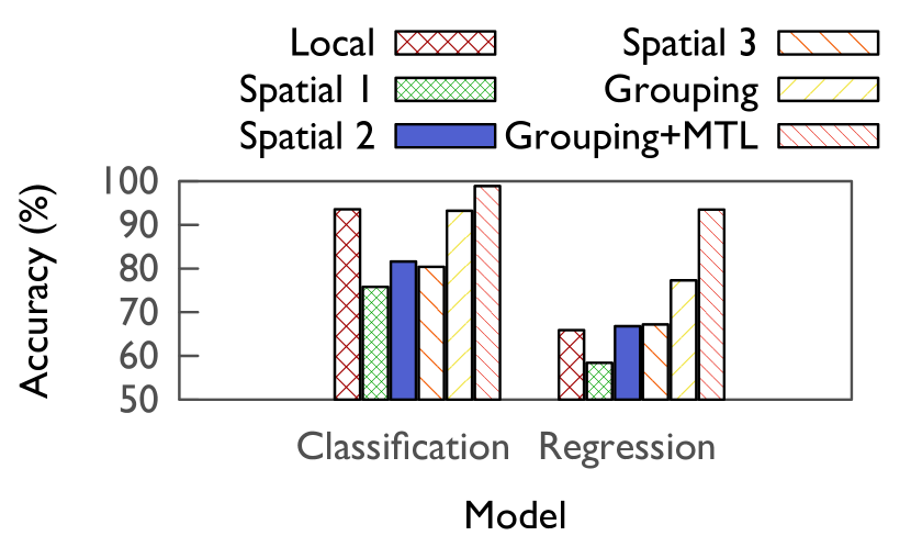
Figure 7: CellScope’s partitioning by itself is able to provide significant gains. MTL provides further gains

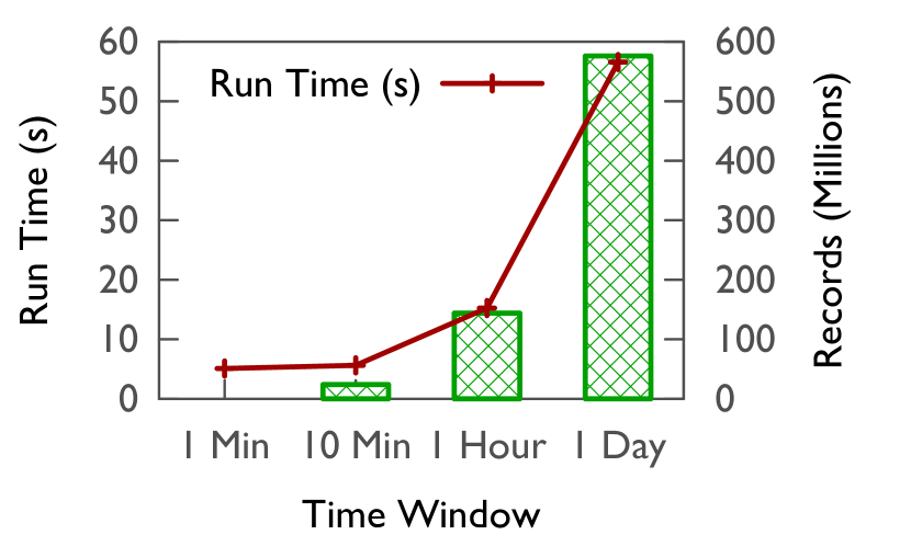
Figure 8: Partitioning overheads are minimal

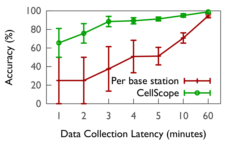
Figure 9: CellScope achieves up to 2.5$\times$ accuracy improvements in drop rate classification

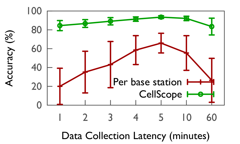
Figure 10: Improvements in throughput model regression go up to 4.4$\times$

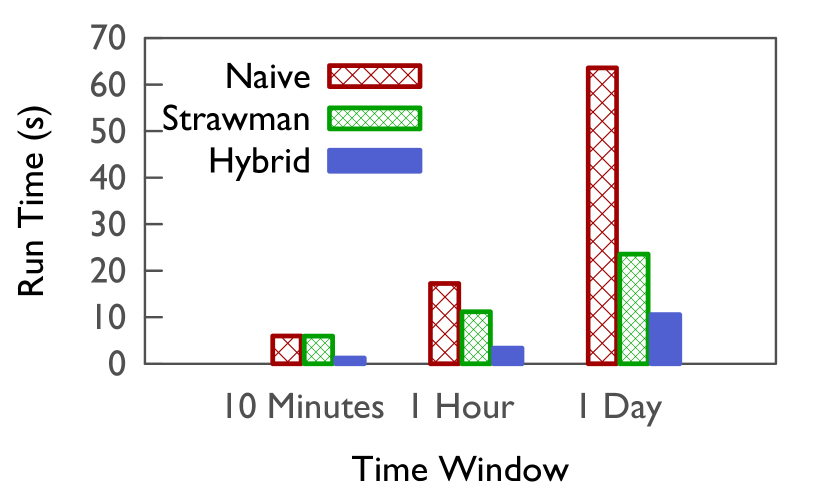
Figure 11: Hyrid model reduces update time by up to 4.8$\times$

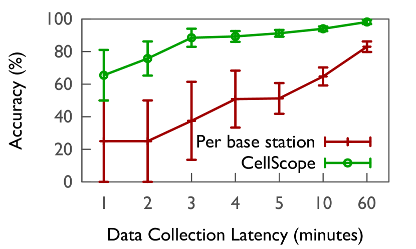
Figure 12: Online training due to the hybrid model helps incur almost no loss in accuracy due to staleness.

Figure 13: CellScope is able to achieve high accuracy while reducing the data collection latency.

We have evaluated CellScope through a series of experiments on real-world cellular traces from a live LTE network from a large geographical area. Our results are summarized below:

• CellScope’s similarity based grouping provides up to 10% improvement in accuracy on its own compared to the best case scenario of space partitioning schemes.

• With MTL, CellScope’s accuracy improvements range from 2.5$\times$ to 4.4$\times$ over different collection latencies.

• Our hybrid online-offline model is able to reduce model update times upto 4.8$\times$ and is able to learn changes in an online fashion with virtually no loss in accuracy.

We discuss these results in detail in the rest of this section.
Evaluation Setup: Due to the sensitive nature of our dataset, our evaluation environment is a private cluster consists of 20 machines. Each machine consists of 4 CPUs, 32GB of memory and a 200GB magnetic hard disk.
Dataset: We collected data from a major metro-area LTE network occupying a large geographical area for a time period of over 10 months. The network serves more than 2 million active users and carries over 6TB of traffic per hour.

6.1 Benefits of Similarity Based Grouping

We first attempt to answer the question "How much benefits do the similarity based grouping provide?". To answer this question, we conducted two experiments, each with a different learning algorithm. The first experiment, whose aim is to detect call drops, uses a classification algorithm while the second, whose aim is to predict throughput, uses a regression algorithm. We chose these to evaluate the benefits in two different classes of algorithms. In both these cases, we pick the data collection latency where the per base station model gives the best accuracy, which was 1 hour for classification and 5 minutes for regression. In order to compare the benefits of our grouping scheme alone, we build a single model per group instead of applying MTL. We compare the accuracy obtained with three different space partitioning schemes. The first scheme (Spatial 1) just partitions space into grids of equal size. The second (Spatial 2) uses a sophisticated space-filling curve based approach [23] that could create dynamically size partitions. Finally, the third (Spatial 3) creates partitions using base stations that are under the same cellular region. The results are shown in fig. 7.

CellScope’s similarity grouping performs as good as the per base station model which gives the highest accuracy. It is interesting to note the performance of spatial partitioning schemes which ranges from 75% to 80%. None of the spatial schemes come close to the similarity grouping results. This is because the drops are few, and concentrated. Spatial schemes club base stations not based on underlying drop characteristics, but only based on spatial proximity. This causes the algorithms to underfit or overfit. Since our similarity based partitioner groups base stations using the drop characteristics, it is able to do as much as 17% better than the spatial schemes.

The benefits are even higher in the regression case. Here, the per base station model is unable to get enough data to build an accurate model and hence is only able to achieve around 66% accuracy. Spatial schemes are able to do slightly better than that. Our similarity based grouping emerges as a clear winner in this case with 77.3% accuracy. This result depicts the highly variable performance characteristics of the base stations, and the need to capture them for accuracy.

These benefits do not come at the cost of higher computational overhead to do the grouping. Figure 8 shows the overhead of performing similarity based grouping on various dataset sizes. It is clear that even very large datasets can be easily partitioned with very little overhead.

6.2 Benefits of MTL

Next, we characterize the benefits of CellScope’s use of MTL. To do this, we repeated the experiment before, and apply MTL to the grouped data to see if the accuracy improves compared to the earlier approach of a single model per group. The results are presented in fig. 7. The ability of MTL to learn and improve models from other similar base stations’ data results in an increase in the accuracy. Over the benefits of grouping, we see an improvement of 6% in the connection drop diagnosis experiment, and 16.2% in the case of throughput prediction experiment. The higher benefits in the latter comes from CellScope’s ability to capture individual characteristics of the base station. This ability is not so crucial in the former because of the limited variation in individual characteristics over those found by the grouping.

6.3 Combined Benefits of Grouping and MTL

We now evaluate the combined benefits of grouping and MTL under different data collection latencies. Here, we are interested in evaluating how CellScope handles the latency accuracy trade-off. To do this, we do the same classification and regression experiments, but on different data collection latencies instead of one. We show the results from the classification experiment in fig. 9 and that from the regression experiment in fig. 10, which compares CellScope’s accuracy against a per base station model’s.

When the opportunity to collect data at individual base stations is limited, CellScope is able to leverage our MTL formulation to combine data from multiple base stations, and build customized models to improve the accuracy. The benefits of CellScope ranges up to 2.5$\times$ in the classification experiment, to 4.4$\times$ in the regression experiment. Lower latencies are problematic in the classification experiment due to the extremely low probability of drops, while higher latencies are a problem in the regression experiment due to the temporal changes in performance characteristics.

6.4 Hybrid model benefits

Finally, we evaluate the benefits of our hybrid modeling. Here, we are interested in learning how much overhead does it reduce during model updates, and can it do online learning.

To answer the first question, we conducted the following experiment: we considered three different data collection latencies: 10 minute, 1 hour and 1 day. We then learn a decision tree model on this data in a tumbling window fashion. So for the 10 minute latency, we collect data for 10 minutes, then build a model, wait another 10 minutes to refine the model and so on. We compare our hybrid model strategy to two different strategies: a naive approach which rebuilds the model from scratch every time, and a better, strawman approach which reuses the last model, and makes changes to it. Both builds a single model while CellScope uses our hybrid MTL model and only updates the online part of the model. The results of this experiment is shown in fig. 11.

The naive approach incurs the highest overhead, which is obvious due to the need to rebuild the entire model from scratch. The overhead increases with the increase in input data. The strawman approach, on the other hand, is able to avoid this heavy overhead. However, it still incurs overheads with larger input because of its use of a single model which requires changes to many parts of the tree. CellScope incurs the least overhead, due to its use of multiple models. When data accumulates, it only needs to update a part of an existing tree, or build a new tree. This strategy results in a reduction of up to 2.2$\times$ to 4.8$\times$ in model building time for CellScope.

To wrap up, we evaluated the performance of the hybrid strategy on different data collection intervals. Here we are interested in seeing if the hybrid model is able to adapt to data changes and provide reasonable accuracies. We use the connection drop experiment again, but do it in a different way. At different collection latencies, we build the model at the beginning of the collection and use the model for the next interval. Hence, for the 1 minute latency, we build a model using the first minute data, and use the model for the second minute (until the whole second minute has arrived). The results are shown in fig. 12. We see here that the per base station model suffers an accuracy loss at higher latencies due to staleness, while CellScope incurs almost zero loss in accuracy. This is because it doesn’t wait until the end of the interval, and is able to incorporate data in real time.

7 RAN Performance Analysis Using CellScope

LTE Physical Layer Parameters
Name	Description
RSRP	Reference Signal Received Power: Average of reference singal power (in watts) across a specified bandwidth. Used for cell selection and handoff.
RSRQ	Reference Signal Recieved Quality: Indicator of interference experienced by the UE. Derived from RSRP and interference metrics.
CQI	Channel Quality Indicator: Carries information on how good/bad communication channel quality is.
SINR	Signal to Interference plus Noise Ratio: Indicates the ratio of the power of the signal to the interference power and background noise.
BLER	Block Error Ratio/Rate: Ratio of the number of erroneous blocks received to the total blocks sent.
PRB	Physical Resource Block: The specific number of subcarriers allocated for a predetermined amount of time for a user.

Table 1: A description of key parameters in LTE physical layer

To validate our system in real world, we now show how domain experts can use CellScope to build efficient RAN performance analysis solutions. To analyze RAN performance, we consider two metrics that are of significant importance for end-user experience: throughput and connection drops. Our findings from the analysis are summarized below:

• Our bearer performance analysis reveals interesting findings on the inefficiencies of P-CQI detection mechanism and link adaptation algorithm. Both of these findings were previously unknown to the operator.

• We find that connection drop is mainly due to uplink SINR and then downlink SINR, and that RSRQ is more reliable than downlink CQI.

• Our cell performance analysis shows that many unknown connection drops can be explained by coverage and uplink interference, and that throughput is seriously impacted by inefficient link adaptation algorithm.

7.1 Analyzing Call Drop Performance

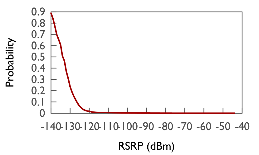
Figure 14: Coverage

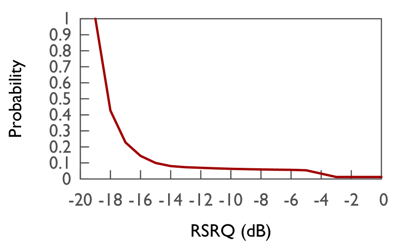
Figure 15: Downlink RSRQ

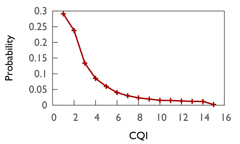
Figure 16: Downlink CQI

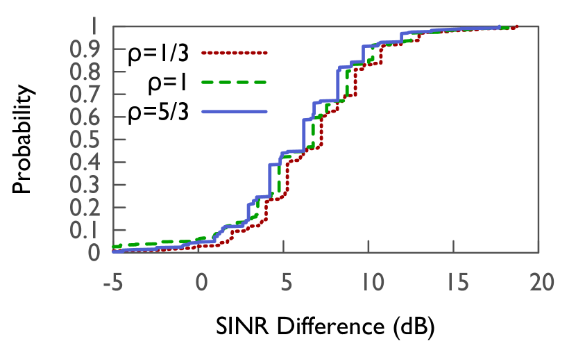
Figure 17: SINR gap

Figure 18: Factors affecting call drops. Although RSRQ and CQI measures downlink interference, they do not match showing an anomaly.

Operators are constantly striving to reduce the amount of drops in the network. With the move towards carrying voice data also over the data network (VoLTE), this metric has gained even more importance. This section describes how we used CellScope to analyze drop performance.

7.1.1 Feature Engineering

Call drops are normally due to one of three metrics:

Coverage It is intuitive to see that poor coverage leads to dropped calls. As seen from fig. 14, areas with $RSRP<-130$ dBm have very high connection drop probability.

Downlink interference For downlink interference, we consider two metrics: RSRQ and downlink CQI. RSRQ is only reported when the UE might need to handoff. CQI is available independent of handoffs. From fig. 15 and fig. 16, we see that the distributions do not match. To reveal the difference of these two distribution, we converted them to the common SINR. To convert CQI, we use the CQI to SINR table. For RSRQ, we use the formula derived in [35], $SINR=\frac{1}{\frac{1}{12RSRQ}-\rho}$. $\rho$ depends on subcarrier utilization. For two antennas, it is between 1/3 and 5/3. For connection failure cases, we show the emperical distribution of their SINR differences with 0%, 50% and 100% subcarrier utilization in fig. 17. We see that 10% has a SINR difference of 10 dB. After revealing our finding to experts, it was discovered that P-CQI feedbacks through physical uplink control channel are not CRC protected. When spurious P-CQIs are received, the physical link adaptation algorithm might choose an incorrect rate resulting in drops.

Uplink interference As shown in fig. 19, the drop probability for uplink SINR has a rather steep slope around and peaks at -17dB. The reason is that the scheduler stops allocating grants at this threshold.

7.1.2 Decision Tree Model for Connection Drops

Based on feature engineering, we picked features that accurately depict call drops. We then used CellScope to train a decision tree that explains the root causes for connection drops. One of the learned trees is shown in fig. 20. As we see, the tree first classifies drops based on uplink SINR, and then makes use of RSRQ if available. We confirmed with experts that the model agrees with their experience. Uplink SINR is more unpredictable because the interference comes from subscribers associated with neighboring base stations. In contrast, downlink interference is from neighboring base stations. CellScope’s models achieved an overall accuracy of $92.1\%$ here, while neither a per base station model nor a global model was able to accurately identify Uplink SINR as the cause and attained less than $80\%$ accuracy.

7.1.3 Detecting Cell KPI Change False Positives Using Concept Drift and Incremental Learning

An interesting application of CellScope’s hybrid model is in detecting false positives of KPI changes. As explained earlier, state-of-the-art performance problem detection systems monitor KPIs, and raise alarms when thresholds are crossed. A major issue with these systems is that the alarms get raised even for known root causes. However, operators cannot confirm this without manual investigation resulting in wasted time and effort. This problem can be solved if known root causes can be filtered out before raising the alarm.

We illustrate this using drop rate. To do so, we use CellScope to apply the decision tree in an incremental fashion on a week worth of data divided into 10 minute interval windows. We used this window length since it matches closely with an interval that is usually used by the operators for monitoring drop rates. In every window, we predict the number of drops using our technique. The predicted drops are explainable, because we know precisely why those drops happened. We use a threshold of $0.5\%$ for the drop rate, hence anything above this threshold is marked as an anomaly. The results from this experiment is depicted in fig. 21. The threshold is exceeded at numerous places. Normally, these would have to be investigated by the expert. However, CellScope explained them to relieve the burden off the operator.

To estimate the confidence in our prediction, we analyzed our results during the occurrence of these anomalies. We consider each connection drop or complete event as a Bernoulli random variable with probability $p$ (from decision tree). A sequence of $n$ connection events follow a binomial distribution. The 95% confidence interval is approximated by $np\pm 2\sqrt{np(1-p)}$. We determine that the alarm is false if $X$ is within the confidence interval. For this particular experiment, the bound was found to be (0.7958665, 0.8610155), thus we conclude that CellScope was successful.

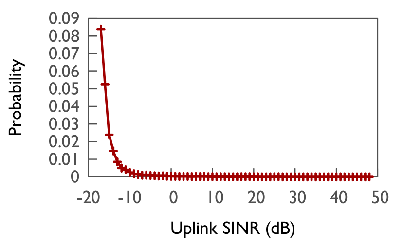
Figure 19: Uplink Interference

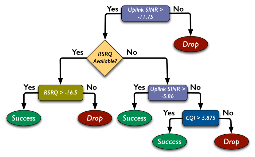
Figure 20: Sample decision tree

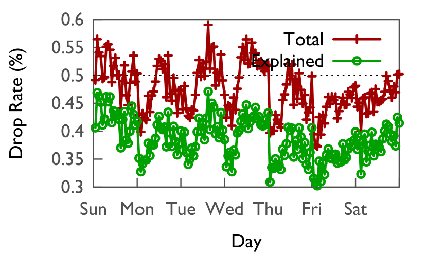
Figure 21: Detecting false Alarms

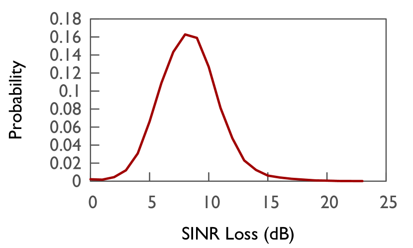
Figure 22: Loss of efficiency

Figure 23: Uplink interference also affects drops. CellScope is able to create local models that accurately detects false alarms.

7.2 Throughput Performance Analysis

Our traces report information that lets us compute RLC throughput as ground truth. We would like to model how far the actual RLC throughput is from the predicted throughput using physical layer and MAC sub-layer information. This helps us understand the contributing factors of throughput.

7.2.1 Feature Engineering

SINR Estimation The base stations have two antennas and are capable of MIMO spatial multiplexing (two streams) or transmit diversity. For both transmissions, each UE reports its two wideband CQIs. We use the CQI to SINR mapping table used at the base station scheduler to convert CQI to SINR. For transmission diversity, we convert the two CQIs to a single SINR as follows. First convert both CQIs to SINR, then compute the two spectrum efficiencies (bits/sec/Hz) using Shannon capacity. We average the two spectrum efficiencies and convert it back to SINR. We then add a 3dB transmission diversity gain to achieve the final SINR. For spatial multiplexing, we convert the two CQIs to two SINRs.

Account for PRB control overhead and BLER target Each PRB is 180 KHz. But not all of it is used for data transmission. For transmit diversity, a 29% overhead is incurred per PRB on average because of resources allocated to physical downlink control channel, broadcast channel and reference signals. The BLER target is 10%.

Account for MAC sub-layer retransmissions The MAC sub-layer performs retransmissions. We denote the MAC efficiency as $\beta_{MAC}$. It is computed as the ratio of total first transmissions over total transmissions. Our traces provide information to compute $\beta_{MAC}$.

7.2.2 Regression Model: Bearer-Level Throughput

The predicted throughput due to transmit diversity is calculated as follows.

$$tput_{RLCdiv} = (1.0-\beta_{MAC})\times 0.9\times(1-0.29)\times 180\times$$

$$PRB_{div}\times log2(1+SINR_{div})/TxTime_{div}$$

$PRB_{div}$ denotes the total PRBs allocated for transmit diversity. $TxTime_{div}$ is the total transmission time for transmit diversity. Similarly we can calculate the predicted throughput due to spatial multiplexing. We then properly weight the two throughput by their respective fraction of transmission time to derive the final RLC throughput.

Account for link adaptation in regression model The base station does not use the SINR corresponding to the UE reported CQI directly. It performs link adaptation to achieve the desired BLER of 10%. This adaptation is necessary since the propagation channel is subject to several conditions, which generally vary in space and time, e.g. path loss, fast fading, UE speed, location (outdoor, indoor, in-car) etc. We add a variable to the throughput equation to account for link adaptation, and use CellScope to learn it along with the other unknowns. Intuitively, this variable indicates how effective the link adaptation algorithm is. Since the base station adjusts a maximum of 6dB, we adjust the SINR used in our prediction by -6dB to compute the lower bound and +6dB to compute the upper bound. We compute the prediction error as follows. If the actual throughput is within the two bounds, the error is zero. If the throughput is outside the two bounds, the error is the distance to the closest bounds. We characterize the difference between the predicted throughput and actual throughput in terms of loss in dB. To compute this, we first convert the actual throughput into SINR. We then subtract the SINR from the one used for throughput prediction. Figure 22 shows that the distribution has a peak around 8dB. As we can see, around 20% of the bearers have a loss of efficiency of more than 10 dB. Due to the high fraction of bearers (20%) with high dB loss (more than 10 dB), we suspect that the link adaptation algorithm is slow to adapt to changing conditions. We validate this finding with field experts. Since this was an unknown insight, they were able to confirm this observation in their lab tests. The reason for this behavior is because the link adaptation algorithm uses the moving average SINR, which is a slow mechanism to adapt.

8 Discussion

We have presented a system that resolves the fundamental trade-off between latency and accuracy in the context of cellular radio network analysis. Now we discuss the deployability and generality of our solution.

Deployability and Impact:

In several domains, it is common to deploy research prototypes on a live system to close the loop. Unfortunately, cellular networks are extremely high business impact systems and hence it is difficult to deploy our system. Nevertheless, our findings were useful for the operator in fixing several issues in their network. Moreover, during this experience, we were able to identify many issues with the data (missing fields, corruptions, incorrect values, etc) and suggest new fields to be added for better diagnostics.

Generality:

Our solutions can be classified into two broad techniques that are applicable to many other domains: partitioning the data by the underlying cause on which the analysis is to be done; and applying domain specific formulations to the analysis approach. It is important to note that MTL is a generic approach. The primary goal of this paper and CellScope is not to apply specific ML algorithms for problem diagnosis, but to propose approaches that enable accurate applications of any ML technique by resolving the latency accuracy trade-off. Thus, we believe that our techniques are general and can be applied to several domains. Some examples of such domains include spatio-temporal analytics and the Internet-of-Things.

9 Related Work

CellScope is related to cellular network monitoring and troubleshooting, self-organizing networks (SON), and network diagnosis techniques and MTL.

Cellular network monitoring and troubleshooting A number of existing cellular network monitoring and diagnosis systems exist [12, 3, 16, 4]. AT&T GigaScope [12] and Alcatel-Lucent Wireless Network Guardian (WNG) [3] generates per IP flow records and monitors many performance metrics such as aggregate per-cell TCP throughput, delay and loss. Because these tools tap interfaces in the core networks, they lack information at the radio access networks. Systems targeting RAN [16, 4] typically monitor aggregate KPIs and per-bearer records separately. Their root cause analysis of KPI problems correlates with aggregation air interface metrics such as SINR histograms and configuration data. Because these systems rely on traditional database technologies, it is hard for them to provide fine-grained prediction based on per-bearer model. In contrast, CellScope is built on top of efficient big data system, Apache Spark. One recent commercial cellular network analytics system [6] adopted the Hadoop big data processing framework. Since it is built on top of WNG [3], it does not have visibility into RANs.
Self-Organizing Networks (SON): The goal of SON [1] is to make the network capable of self-configuration (e.g. automatic neighbor list configuration) and self-optimization. CellScope focuses on understanding RAN performance and assists troubleshooting, thus can be used to assist SON.
Modelling and diagnosis techniques: Diagnosing problems in cellular networks has been explored in the literature in various forms [8, 22, 29, 33, 43], where the focus of the work has either been detecting faults or finding the root cause of failures. A probabilistic system for auto-diagnosing faults in RAN is presented in  [8]. It relies on KPIs. However, KPIs are not capable of providing diagnosis at high granularity. Moreover, it is unclear how their proposals capture complex dependencies between different components in RAN. An automated approach to locating anomalous events on hierarchical operational networks was proposed in [22] based on hierarchical heavy hitter based anomaly detection. It is unclear how their proposals carry over to RAN. Adding autonomous capabilities to alarm based fault detection is discussed in [29]. While their techniques can help systems auto-heal faults, correlation based fault detection is insufficient for fine granularity detection and diagnosis of faults. [33] looks at detecting call connection faults due to load imbalances. In [47], a technique to detect and localize anomalies from an ISP point of view is proposed. Finally, [43] discusses the use of ML tools in predicting call drops and its duration.
Multi-Task Learning: MTL builds on the idea that related tasks can learn from each other to achieve better statistical efficiency [10, 44, 17, 9]. Since the assumption of task relatedness do not hold in many scenarios, techniques to automatically cluster tasks have been explored in the past [25, 20]. However, these techniques consider tasks as black boxes and hence cannot leverage domain specific structure. In contrast, CellScope proposes a hybrid offline-online MTL formulation on a domain-specific grouping of tasks based on underlying performance characteristics.

10 Conclusion and Future Work

While several domains can benefit from analyzing data collected in a real-time fashion, the practicality of these analyses are impeded by a fundamental trade-off between data collection latency and analysis accuracy. In this paper, we explored this trade-off in the context of a specific domain use-case, performance analysis in cellular RANs. We presented CellScope to resolve this trade-off by applying a domain specific formulation of MTL. CellScope first transforms raw data into insightful features. To apply MTL effectively, CellScope proposed a novel PCA inspired similarity metric that groups data from geographically nearby base stations sharing performance commonalities. Finally, it also incorporates a hybrid online-offline model for efficient model updates. We have built CellScope on Apache Spark and evaluated it on real data that shows accuracy improvements ranging from 2.5$\times$ to 4.4$\times$ over direct applications of ML. We have also used CellScope to analyze a live LTE consisting of over 2 million subscribers for a period of over 10 months, where it uncovered several problems and insights.

For future work, we wish to explore the applicability of our techniques for resolving the trade-off in other domains where similarity based grouping is possible. Further, since our design is amenable to geo-distributed learning, we wish to investigate the trade-offs in such settings.

References

- [1] 3gpp. Self-organizing networks son policy network resource model (nrm) integration reference point (irp). http://www.3gpp.org/ftp/Specs/archive/32_series/32.521/.
- [2] Aggarwal, B., Bhagwan, R., Das, T., Eswaran, S., Padmanabhan, V. N., and Voelker, G. M. Netprints: diagnosing home network misconfigurations using shared knowledge. In Proceedings of the 6th USENIX symposium on Networked systems design and implementation (Berkeley, CA, USA, 2009), NSDI’09, USENIX Association, pp. 349–364.
- [3] Alcatel Lucent. 9900 wireless network guardian. http://www.alcatel-lucent.com/products/9900-wireless-network-guardian, 2013.
- [4] Alcatel Lucent. 9959 network performance optimizer. http://www.alcatel-lucent.com/products/9959-network-performance-optimizer, 2014.
- [5] Alcatel Lucent. Alcatel-Lucent motive big network analytics for service creation. http://resources.alcatel-lucent.com/?cid=170795, 2014.
- [6] Alcatel Lucent. Motive big network analytics. http://www.alcatel-lucent.com/solutions/motive-big-network-analytics, 2014.
- [7] Bahl, P., Chandra, R., Greenberg, A., Kandula, S., Maltz, D. A., and Zhang, M. Towards highly reliable enterprise network services via inference of multi-level dependencies. In Proceedings of the 2007 Conference on Applications, Technologies, Architectures, and Protocols for Computer Communications (New York, NY, USA, 2007), SIGCOMM ’07, ACM, pp. 13–24.
- [8] Barco, R., Wille, V., Díez, L., and Toril, M. Learning of model parameters for fault diagnosis in wireless networks. Wirel. Netw. 16, 1 (Jan. 2010), 255–271.
- [9] Baxter, J. A model of inductive bias learning. J. Artif. Int. Res. 12, 1 (Mar. 2000), 149–198.
- [10] Caruana, R. Multitask learning: A knowledge-based source of inductive bias. In Proceedings of the Tenth International Conference on Machine Learning (1993), Morgan Kaufmann, pp. 41–48.
- [11] Cohen, I., Goldszmidt, M., Kelly, T., Symons, J., and Chase, J. S. Correlating instrumentation data to system states: A building block for automated diagnosis and control. In Proceedings of the 6th Conference on Symposium on Opearting Systems Design & Implementation - Volume 6 (Berkeley, CA, USA, 2004), OSDI’04, USENIX Association, pp. 16–16.
- [12] Cranor, C., Johnson, T., Spataschek, O., and Shkapenyuk, V. Gigascope: a stream database for network applications. In Proceedings of the 2003 ACM SIGMOD international conference on Management of data (New York, NY, USA, 2003), SIGMOD ’03, ACM, pp. 647–651.
- [13] Dietterich, T. G. Ensemble methods in machine learning. In Multiple classifier systems. Springer, 2000, pp. 1–15.
- [14] Eljaam, B. Customer satisfaction with cellular network performance: Issues and analysis.
- [15] Ericsson. Ericsson RAN analyzer overview. http://www.optxview.com/Optimi_Ericsson/RANAnalyser.pdf, 2012.
- [16] Ericsson. Ericsson RAN analyzer. http://www.ericsson.com/ourportfolio/products/ran-analyzer, 2014.
- [17] Evgeniou, T., and Pontil, M. Regularized multi–task learning. In Proceedings of the Tenth ACM SIGKDD International Conference on Knowledge Discovery and Data Mining (New York, NY, USA, 2004), KDD ’04, ACM, pp. 109–117.
- [18] Friedman, J. H. Greedy function approximation: a gradient boosting machine. Annals of statistics (2001), 1189–1232.
- [19] Gama, J. a., Žliobaitė, I., Bifet, A., Pechenizkiy, M., and Bouchachia, A. A survey on concept drift adaptation. ACM Comput. Surv. 46, 4 (Mar. 2014), 44:1–44:37.
- [20] Gong, P., Ye, J., and Zhang, C. Robust multi-task feature learning. In Proceedings of the 18th ACM SIGKDD International Conference on Knowledge Discovery and Data Mining (New York, NY, USA, 2012), KDD ’12, ACM, pp. 895–903.
- [21] Harris, P., Brunsdon, C., and Charlton, M. Geographically weighted principal components analysis. International Journal of Geographical Information Science 25, 10 (2011), 1717–1736.
- [22] Hong, C.-Y., Caesar, M., Duffield, N., and Wang, J. Tiresias: Online anomaly detection for hierarchical operational network data. In Proceedings of the 2012 IEEE 32Nd International Conference on Distributed Computing Systems (Washington, DC, USA, 2012), ICDCS ’12, IEEE Computer Society, pp. 173–182.
- [23] Iyer, A., Li, L. E., and Stoica, I. Celliq : Real-time cellular network analytics at scale. In 12th USENIX Symposium on Networked Systems Design and Implementation (NSDI 15) (Oakland, CA, May 2015), USENIX Association, pp. 309–322.
- [24] Khanna, G., Yu Cheng, M., Varadharajan, P., Bagchi, S., Correia, M. P., and Veríssimo, P. J. Automated rule-based diagnosis through a distributed monitor system. IEEE Trans. Dependable Secur. Comput. 4, 4 (Oct. 2007), 266–279.
- [25] Kim, S., and Xing, E. P. Tree-guided group lasso for multi-task regression with structured sparsity. Intenational Conference on Machine Learning (ICML) (2010).
- [26] Kraska, T., Talwalkar, A., Duchi, J. C., Griffith, R., Franklin, M. J., and Jordan, M. I. Mlbase: A distributed machine-learning system. In CIDR (2013).
- [27] Krzanowski, W. Between-groups comparison of principal components. Journal of the American Statistical Association 74, 367 (1979), 703–707.
- [28] Lakhina, A., Crovella, M., and Diot, C. Diagnosing network-wide traffic anomalies. In Proceedings of the 2004 Conference on Applications, Technologies, Architectures, and Protocols for Computer Communications (New York, NY, USA, 2004), SIGCOMM ’04, ACM, pp. 219–230.
- [29] Liu, Y., Zhang, J., Jiang, M., Raymer, D., and Strassner, J. A model-based approach to adding autonomic capabilities to network fault management system. In Network Operations and Management Symposium, 2008. NOMS 2008. IEEE (April 2008), pp. 859–862.
- [30] Murphy, K. P. Machine learning: a probabilistic perspective. MIT press, 2012.
- [31] Pan, Y., Xia, R., Yin, J., and Liu, N. A divide-and-conquer method for scalable robust multitask learning. Neural Networks and Learning Systems, IEEE Transactions on 26, 12 (Dec 2015), 3163–3175.
- [32] Pearson, K. On lines and planes of closest fit to systems of points in space. Philosophical Magazine 2, 6 (1901), 559–572.
- [33] Rao, S. Operational fault detection in cellular wireless base-stations. IEEE Trans. on Netw. and Serv. Manag. 3, 2 (Apr. 2006), 1–11.
- [34] Safwat, A. M., and Mouftah, H. 4g network technologies for mobile telecommunications. Network, IEEE 19, 5 (2005), 3–4.
- [35] Salo, J. Mobility parameter planning for 3GPP LTE: Basic concepts and intra-layer mobility. www.lteexpert.com/lte_mobility_wp1_10June2013.pdf.
- [36] Sesia, S., Toufik, I., and Baker, M. LTE: the UMTS long term evolution. Wiley Online Library, 2009.
- [37] Shafiq, M. Z., Erman, J., Ji, L., Liu, A. X., Pang, J., and Wang, J. Understanding the impact of network dynamics on mobile video user engagement. In The 2014 ACM International Conference on Measurement and Modeling of Computer Systems (New York, NY, USA, 2014), SIGMETRICS ’14, ACM, pp. 367–379.
- [38] Shafiq, M. Z., Ji, L., Liu, A. X., Pang, J., Venkataraman, S., and Wang, J. A first look at cellular network performance during crowded events. In Proceedings of the ACM SIGMETRICS/International Conference on Measurement and Modeling of Computer Systems (New York, NY, USA, 2013), SIGMETRICS ’13, ACM, pp. 17–28.
- [39] Shalev-Shwartz, S., and Tewari, A. Stochastic methods for l1-regularized loss minimization. J. Mach. Learn. Res. 12 (July 2011), 1865–1892.
- [40] Smith, C. 3G wireless networks. McGraw-Hill, Inc., 2006.
- [41] Sparks, E. R., Talwalkar, A., Smith, V., Kottalam, J., Pan, X., Gonzalez, J. E., Franklin, M. J., Jordan, M. I., and Kraska, T. MLI: an API for distributed machine learning. In 2013 IEEE 13th International Conference on Data Mining, Dallas, TX, USA, December 7-10, 2013 (2013), H. Xiong, G. Karypis, B. M. Thuraisingham, D. J. Cook, and X. Wu, Eds., IEEE Computer Society, pp. 1187–1192.
- [42] Technical Specification Group. 3gpp specifications. http://www.3gpp.org/specifications.
- [43] Theera-Ampornpunt, N., Bagchi, S., Joshi, K. R., and Panta, R. K. Using big data for more dependability: A cellular network tale. In Proceedings of the 9th Workshop on Hot Topics in Dependable Systems (New York, NY, USA, 2013), HotDep ’13, ACM, pp. 2:1–2:5.
- [44] Thrun, S. Is learning the n-th thing any easier than learning the first? In Advances in Neural Information Processing Systems (1996), The MIT Press, pp. 640–646.
- [45] Tibshirani, R. Regression shrinkage and selection via the lasso. Journal of the Royal Statistical Society, Series B 58 (1994), 267–288.
- [46] Wang, H. J., Platt, J. C., Chen, Y., Zhang, R., and Wang, Y.-M. Automatic misconfiguration troubleshooting with peerpressure. In Proceedings of the 6th Conference on Symposium on Opearting Systems Design & Implementation - Volume 6 (Berkeley, CA, USA, 2004), OSDI’04, USENIX Association, pp. 17–17.
- [47] Yan, H., Flavel, A., Ge, Z., Gerber, A., Massey, D., Papadopoulos, C., Shah, H., and Yates, J. Argus: End-to-end service anomaly detection and localization from an isp’s point of view. In INFOCOM, 2012 Proceedings IEEE (2012), pp. 2756–2760.
- [48] Yang, K., and Shahabi, C. A pca-based similarity measure for multivariate time series. In Proceedings of the 2nd ACM International Workshop on Multimedia Databases (New York, NY, USA, 2004), MMDB ’04, ACM, pp. 65–74.
- [49] Zaharia, M., Chowdhury, M., Das, T., Dave, A., Ma, J., McCauley, M., Franklin, M. J., Shenker, S., and Stoica, I. Resilient distributed datasets: a fault-tolerant abstraction for in-memory cluster computing. In Proceedings of the 9th USENIX conference on Networked Systems Design and Implementation (Berkeley, CA, USA, 2012), NSDI’12, USENIX Association, pp. 2–2.
- [50] Zaharia, M., Das, T., Li, H., Hunter, T., Shenker, S., and Stoica, I. Discretized streams: Fault-tolerant streaming computation at scale. In Proceedings of the Twenty-Fourth ACM Symposium on Operating Systems Principles (New York, NY, USA, 2013), SOSP ’13, ACM, pp. 423–438.
- [51] Zhang, C., Kumar, A., and Ré, C. Materialization optimizations for feature selection workloads. In Proceedings of the 2014 ACM SIGMOD International Conference on Management of Data (New York, NY, USA, 2014), SIGMOD ’14, ACM, pp. 265–276.
- [52] Zheng, A. X., Lloyd, J., and Brewer, E. Failure diagnosis using decision trees. In Proceedings of the First International Conference on Autonomic Computing (Washington, DC, USA, 2004), ICAC ’04, IEEE Computer Society, pp. 36–43.