Efficient Construction of Probabilistic Tree Embeddings

Abstract

In this paper we describe an algorithm that embeds a graph metric $(V,d_{G})$ on an undirected weighted graph $G=(V,E)$ into a distribution of tree metrics $(T,D_{T})$ such that for every pair $u,v\in V$, $d_{G}(u,v)\leq d_{T}(u,v)$ and $\operatorname{\bf{E}}_{T}[d_{T}(u,v)]\leq O(\log n)\cdot d_{G}(u,v)$. Such embeddings have proved highly useful in designing fast approximation algorithms, as many hard problems on graphs are easy to solve on tree instances. For a graph with $n$ vertices and $m$ edges, our algorithm runs in $O(m\log n)$ time with high probability, which improves the previous upper bound of $O(m\log^{3}n)$ shown by Mendel et al. in 2009.

The key component of our algorithm is a new approximate single-source shortest-path algorithm, which implements the priority queue with a new data structure, the bucket-tree structure. The algorithm has three properties: it only requires linear time in the number of edges in the input graph; the computed distances have a distance preserving property; and when computing the shortest-paths to the $k$-nearest vertices from the source, it only requires to visit these vertices and their edge lists. These properties are essential to guarantee the correctness and the stated time bound.

Using this shortest-path algorithm, we show how to generate an intermediate structure, the approximate dominance sequences of the input graph, in $O(m\log n)$ time, and further propose a simple yet efficient algorithm to converted this sequence to a tree embedding in $O(n\log n)$ time, both with high probability. Combining the three subroutines gives the stated time bound of the algorithm.

Then we show that this efficient construction can facilitate some applications. We proved that FRT trees (the generated tree embedding) are Ramsey partitions with asymptotically tight bound, so the construction of a series of distance oracles can be accelerated.

1 Introduction

The idea of probabilistic tree embeddings [4] is to embed a finite metric into a distribution of tree metrics with a minimum expected distance distortion. A distribution $\mathcal{D}$ of trees of a metric space $(X,d_{X})$ should minimize the expected stretch $\psi$ so that:

1. dominating property: for each tree $T\in\mathcal{D}$, $d_{X}(x,y)\leq d_{T}(x,y)$ for every $x,y\in X$, and

2. expected stretch bound: $\operatorname{\bf{E}}_{T\sim\mathcal{D}}[d_{T}(x,y)]\leq\psi\cdot d_{X}(x,y)$ for every $x,y\in X$,

where $d_{T}(\cdot,\cdot)$ is the tree metric, and $\operatorname{\bf{E}}_{T\sim\mathcal{D}}$ draws a tree $T$ from the distribution $\mathcal{D}$. After a sequence of results [2, 3, 4], Fakcharoenphol, Rao and Talwar [16] eventually proposed an elegant and asymptotically optimal algorithm (FRT-embedding) with $\psi=O(\log n)$.

Probabilistic tree embeddings facilitate many applications. They lead to practical algorithms to solve a number of problems with good approximation bounds, for example, the $k$-median problem, buy-at-bulk network design [7], and network congestion minimization [31]. A number of network algorithms use tree embeddings as key components, and such applications include generalized Steiner forest problem, the minimum routing cost spanning tree problem, and the $k$-source shortest paths problem [22]. Also, tree embeddings are used in solving symmetric diagonally dominant (SDD) linear systems. Classic solutions use spanning trees as the preconditioner, but recent work by Cohen et al. [13] describes a new approach to use trees with Steiner nodes (e.g. FRT trees).

In this paper we discuss yet another remarkable application of probabilistic tree embeddings: constructing of approximate distance oracles (ADOs)—a data structure with compact storage ($o(n^{2})$) which can approximately and efficiently answer pairwise distance queries on a metric space. We show that FRT trees can be used to accelerate the construction of some ADOs [25, 35, 9].

Motivated by these applications, efficient algorithms to construct tree embeddings are essential, and there are several results on the topic in recent years [11, 22, 7, 26, 20, 18, 6]. Some of these algorithms are based on different parallel settings, e.g. share-memory setting [7, 18, 6] or distributed setting [22, 20]. As with this paper, most of these algorithms [11, 22, 26, 20, 6] focus on graph metrics, which most of the applications discussed above are based on. In the sequential setting, i.e. on a RAM model, to the best of our knowledge, the most efficient algorithm to construct optimal FRT-embeddings was proposed by Mendel and Schwob [26]. It constructs FRT-embeddings in $O(m\log^{3}n)$ expected time given an undirected positively weighted graph with $n$ vertices and $m$ edges. This algorithm, as well as the original construction in the FRT paper [16], works hierarchically by generating each level of a tree top-down. However, such a method can be expensive in time and/or coding complexity. The reason is that the diameter of the graph can be arbitrarily large and the FRT trees may contain many levels, which requires complicated techniques, such as building sub-trees based on quotient graphs.

Our results. The main contribution of this paper is an efficient construction of the FRT-embeddings. Given an undirected positively weighted graph $G=(V,E)$ with $n$ vertices and $m$ edges, our algorithm builds an optimal tree embedding in $O(m\log n)$ time. In our algorithm, instead of generating partitions by level, we adopt an alternative view of the FRT algorithm in [22, 7], which computes the potential ancestors for each vertex using dominance sequences of a graph (first proposed in [11], and named as least-element lists in [11, 22]). The original algorithm to compute the dominance sequences requires $O(m\log n+n\log^{2}n)$ time [11]. We then discuss a new yet simple algorithm to convert the dominance sequences to an FRT tree only using $O(n\log n)$ time. A similar approach was taken by Khan et al. [22] but their output is an implicit representation (instead of an tree) and under the distributed setting and it is not work-efficient without using the observations and tree representations introduced by Blelloch et al. in [7].

Based on the algorithm to efficiently convert the dominance sequences to FRT trees, the time complexity of FRT-embedding construction is bottlenecked by the construction of the dominance sequences. Our efficient approach contains two subroutines:

• An efficient (approximate) single-source shortest-path algorithm, introduced in Section 3. The algorithm has three properties: linear complexity, distance preservation, and the ordering property (full definitions given in Section 3). All three properties are required for the correctness and efficiency of constructing FRT-embedding. Our algorithm is a variant of Dijkstra’s algorithm with the priority queue implemented by a new data structure called leveled bucket structure.

• An algorithm to integrate the shortest-path distances into the construction of FRT trees, discussed in Section 4. When the diameter of the graph is $n^{O(1)}$, we show that an FRT tree can be built directly using the approximate distances computed by shortest-path algorithm. The challenge is when the graph diameter is large, and we proposed an algorithm that computes the approximate dominance sequences of a graph by concatenating the distances that only use the edges within a relative range of $n^{O(1)}$. Then we show why the approximate dominance sequences still yield valid FRT trees.

With these new algorithmic subroutines, we show that the time complexity of computing FRT-embedding can be reduced to $O(m\log n)$ w.h.p. for an undirected positively weighted graph with arbitrary edge weight.

The second contribution of this paper is to show a new application of optimal probabilistic tree embeddings. We show that FRT trees are intrinsically Ramsey partitions (definition given in Section 5) with asymptotically tight bound, and can achieve even better (constant) bounds on distance approximation. Previous construction algorithms of optimal Ramsey partitions are based on hierarchical CKR partitions, namely, on each level, the partition is individually generated with an independent random radius and new random priorities. In this paper, we present a new proof to show that the randomness in each level is actually unnecessary, so that only one single random permutation is enough and the ratio of radii in consecutive levels can be fixed as 2. Our FRT-tree construction algorithm therefore can be directly applied to a number of different distance oracles that are based on Ramsey partitions and accelerates the construction of these distance oracles.

2 Preliminaries and Notations

Let $G=(V,E)$ be a weighted graph with edge weights $w:E\rightarrow\mathbb{R}_{+}$, and $d(u,v)$ denote the shortest-path distance in $G$ between nodes $u$ and $v$. Throughout this paper, we assume that $\min_{x\neq y}d(x,y)=1$. Let $\Delta={\max_{x,y}d(x,y)\over\min_{x\neq y}d(x,y)}=\max_{x,y}d(x,y)$, the diameter of the graph $G$.

In this paper, we use the single source shortest paths problem (SSSP) as a subroutine for a number of algorithms. Consider a weighted graph with $n$ vertices and $m$ edges, Dijkstra’s algorithm [14] solves the SSSP in $O(m+n\log n)$ time if the priority queue of distances is maintained using a Fibonacci heap [17].

A premetric $(X,d_{X})$ defines on a set $X$ and provides a function $d:X\times X\to\mathbb{R}$ satisfying $d(x,x)=0$ and $d(x,y)\geq 0$ for $x,y\in X$. A metric $(X,d_{X})$ further requires $d(x,y)=0$ iff $x=y$, symmetry $d(x,y)=d(y,x)$, triangle inequality $d(x,y)\leq d(x,z)+d(z,y)$ for $x,y,z\in X$. The shortest-path distances on a graph is a metric and is called the graph metric and denoted as $d_{G}$.

We assume all intermediate results of our algorithm have word size $O(\log n)$ and basic algorithmic operations can be finished within a constant time. Then within the range of $[1,n^{k}]$, the integer part of natural logarithm of an integer and floor function of an real number can be computed in constant time for any constant $k$. This can be achieved using standard table-lookup techniques (similar approaches can be found in Thorup’s algorithm [33]). The time complexity of the algorithms are measured using the random-access machine (RAM) model.

A result holds with high probability (w.h.p.) for an input of size $n$ if it holds with probability at least $1-n^{-c}$ for any constant $c>0$, over all possible random choices made by the algorithm.

Let $[n]=\{1,2,\cdots,n\}$ where $n$ is a positive integer.

Let $(X,d_{X})$ be a metric space. For $Y\subseteq X$, define $(Y,d_{X})$ as the metric $d_{X}$ restricted to pairs of points in $Y$, and $\operatorname{diam}(Y,d_{X})=\max\{d_{X}(x,y)\mid x,y\in Y\}$. Define $B_{X}(x,r)=\{y\in X\mid d_{X}(x,y)\leq r\}$, the closed ball centered at point $x$ and containing all points in $X$ at a distance of at most $r$ from $x$. A partition $\mathcal{P}$ of $X$ is a set of subsets of $X$ such that, for every $x\in X$, there is one and only one unique element in $\mathcal{P}$, denoted as $\mathcal{P}(x)$, that contains $x$.

The KR-expansion constant [21] of a given metric space $(X,d_{X})$ is defined as the smallest value of $c\geq 2$ such that $\mathopen{}\mathclose{{}\left|B_{X}(x,2r)}\right|\leq c\cdot\mathopen{}\mathclose{{}\left|B_{X}(x,r)}\right|$ for all $x\in X$ and $r>0$. The KR-dimension [21] (or the expansion dimension) of $X$ is defined as $\dim_{{\mbox{\scriptsize\emph{KR}}}}(X)=\log c$.

We recall a useful fact about random permutations [32]:

Lemma 2.1.

Let $\pi:[n]\rightarrow[n]$ be a permutation selected uniformly at random on $[n]$. The set $\{i\mid i\in[n],\pi(i)=\min\{\pi(j)\mid j=1,\cdots,i\}\}$ contains $O(\log n)$ elements both in expectation and with high probability.

Ramsey partitions.

Let $(X,d_{X})$ be a metric space. A hierarchical partition tree of $X$ is a sequence of partitions $\{\mathcal{P}_{k}\}_{k=0}^{\infty}$ of $X$ such that $\mathcal{P}_{0}=\{X\}$, the diameter of the partitions in each level decreases by a constant $c>1$, and each level $\mathcal{P}_{k+1}$ is a refinement of the previous level $\mathcal{P}_{k}$. A Ramsey partition [25] is a distribution of hierarchical partition trees such that each vertex has a lower-bounded probability of being sufficiently far from the partition boundaries in all partitions $k$, and this gap is called the padded range of a vertex. More formally:

Definition 1.

An $(\alpha,\gamma)$-Ramsey partition of a metric space $(X,d_{X})$ is a probability distribution over hierarchical partition trees $\mathcal{P}$ of $X$ such that for every $x\in X$:

$$\Pr\mathopen{}\mathclose{{}\left[\forall k\in\mathbb{N},B_{X}\mathopen{}\mathclose{{}\left(x,\alpha\cdot c^{-k}\Delta}\right)\subseteq\mathcal{P}_{k}(x)}\right]\geq|X|^{-\gamma}.$$

An asymptotically tight construction of Ramsey partition where $\alpha=\Omega(\gamma)$ is provided by Mendel and Naor [25] using the Calinescu-Karloff-Rabani partition [8] for each level.

Approximate distance oracles.

Given a finite metric space $(X,d_{X})$, we want to support efficient approximate pairwise shortest-distance queries. Data structures to support this query are called approximate distance oracles. A $(P,S,Q,D)$-distance oracle on a finite metric space $(X,d_{X})$ is a data structure that takes expected time $P$ to preprocess from the given metric space, uses $S$ storage space, and answers distance query between points $x$ and $y$ in $X$ in time $Q$ satisfying $d_{X}(x,y)\leq d_{O}(x,y)\leq D\cdot d_{X}(x,y)$, where $d_{O}(x,y)$ is the pairwise distance provided by the distance oracle.

The concept of approximate distance oracles was first studied by Thorup and Zwick [34]. Their distance oracles are based on graph spanners, and given a graph, a $(O(kmn^{1/k}),O(kn^{1+1/k}),O(k),2k-1)$-oracle can be created. This was followed by many improved results, including algorithms focused on distance oracles that provide small stretches ($<3$) [5, 1], and oracles that can report paths in addition to distances [15]. A recent result of Chechik [10] provides almost optimal space, stretch and query time, but the construction time is polynomially slower than the results in this paper, and some of the other work, when $k>2$.

For distance oracles that can be both constructed and queried efficiently on a graph, a series of algorithms, including Mendel-Naor’s [25], Wulff-Nilsen’s [35] and Chechik’s [9], all use the Ramsey partitions of a graph as an algorithmic building block of the algorithm.

3 An Approximate SSSP Algorithm

In this section we introduce a variant of Dijkstra’s algorithm. This is an efficient algorithm for single-source shortest paths (SSSP) with linear time complexity $O(m)$. The computed distances are $\alpha$-distance preserving:

Definition 2 ($\alpha$-distance preserving).

For a weighted graph $G=(V,E)$, the single-source distances $d(v)$ for $v\in V$ from the source node $s$ is $\alpha$-distance preserving, if there exists a constant $0\leq\alpha\leq 1$ such that $\alpha\,d_{G}(s,u)\leq d(u)\leq d_{G}(s,u)$, and $d(v)-d(u)\leq d_{G}(u,v)$, for every $u,v\in V$.

$\alpha$-distance preserving can be viewed as the triangle inequality on single-source distances (i.e. $d(u)+d_{G}(u,v)\geq d(v)$ for $u,v\in V$), and is required in many applications related to distances. For example, in Corollary 3.2 we show that using Gabow’s scaling algorithm [19] we can compute a ($1-\epsilon$)-approximate SSSP using $O(m\log\epsilon^{-1})$ time. Also in many metric problems including the contruction of optimal tree embeddings, distance preservation is necessary in the proof of the expected stretch, and such an example is Lemma 4.3 in Section 4.3.

The preliminary version we discussed in Section 3.1 limits edge weights in $[1,n^{k}]$ for a constant $k$, but with some further analysis in the full version of this paper we can extend the range to $[1,n^{O(m)}]$. This new algorithm also has two properties that are needed in the construction of FRT trees, while no previous algorithms achieve them all:

1. ($\alpha$-distance preserving) The computed distances from the source $d(\cdot)$ is $\alpha$-distance preserving.

2. (Ordering property and linear complexity) The vertices are visited in order of distance $d(\cdot)$, and the time to compute the first $k$ distances is bounded by $O(m^{\prime})$ where $m^{\prime}$ is the sum of degrees from these $k$ vertices.

The algorithm also works on directed graphs, although this is not used in the FRT construction.

Approximate SSSP algorithms are well-studied [33, 23, 12, 30, 27]. In the sequential setting, Thorup’s algorithm [33] compute single-source distances on undirected graphs with integer weights using $O(n+m)$ time. Nevertheless, Thorup’s algorithm does not obey the ordering property since it uses a hierarchical bucketing structure and does not visit vertices in an order of increasing distances, and yet we are unaware of a simple argument to fix this. Other algorithms are either not work-efficient (i.e. super-linear complexity) in sequential setting, and / or violating distance preservation.

Theorem 3.1.

For a weighted directed graph $G=(V,E)$ with edge weights between $1$ and $n^{O(1)}$, a $(1/4)$-distance preserving single-source shortest-path distances $d(\cdot)$ can be computed, such that the distance to the $k$-nearest vertices $v_{1}$ to $v_{k}$ by $d(\cdot)$requires $O(\sum_{i=1}^{k}{{\mbox{\emph{degree}}}(v_{i})})$ time.

The algorithm also has the two following properties. We discuss how to (1) extend the range of edge weights to $n^{O(m)}$, and the cost to compute the $k$-nearest vertices is $O(\log_{n}{d(v_{k})}+\sum_{i=1}^{k}{{\mbox{\emph{degree}}}(v_{i})})$ where $v_{1}$ to $v_{k}$ are the $k$ nearest vertices (Section 3.2); and (2) compute $(1+\epsilon)$-distance-preserving shortest-paths for an arbitrary $\epsilon>0$:

Corollary 3.2.

For a graph $G=(V,E)$ and any source $s\in V$, $(1-\epsilon)$-distance-preserving approximate distances $d(v)$ for $v\in V$ from $s$, can be computed by repeatedly using the result of Theorem 3.1 $O(\log\epsilon^{-1})$ rounds, which leads to $O(mlog\epsilon^{-1})$ when edge weights are within $n^{O(1)}$.

$(1-\epsilon)$-distance-preserving shortest-paths for all vertices can be computed by repeatedly using Theorem 3.1 $O(\log\epsilon^{-1})$ rounds.

Proof.

To get $(1-\epsilon)$-distance-preserving shortest-paths, we can use the algorithm in Theorem 3.1 $O(\log\epsilon^{-1})$ rounds repeatedly, and the output shortest-paths in $i$-th round are denoted as $d_{i}(\cdot)$. The first round is run on the input graph. In the $i$-th round for $i>1$, each edge $e$ from $u$ to $v$ in the graph is reweighted as $w_{e}+\sum_{j=1}^{i}(d_{j}(u)-d_{j}(v))$. Since we know that the output is distance preserving for the input graph in each round, inductively we can check that all reweighted edges are positive. This also indicates that $\sum_{j=1}^{i}d_{j}(u)\leq d(s,u)$.

We now show that, from source node $s$, $d(s,u)-\sum_{j=1}^{i}d_{j}(u)\leq(1-\alpha)^{i}\cdot d(s,u)$. This is because, by running the shortest-path algorithm that is $\alpha$-distance preserving, $d_{i}(u)\geq\alpha\cdot(d(s,u)-\sum_{j=1}^{i-1}d_{j}(u))$ based on the way the graph is reweighted. Therefore, the summation of all $d_{i}(u)$ is at least $(1-\epsilon)\,d(s,u)$ after $O(\log\epsilon^{-1})$ rounds. ∎

3.1 Algorithm Details

The key data structure in this algorithm is a leveled bucket structure shown in Figure 1 that implements the priority queue in Dijkstra’s algorithm. With the leveled bucket structure, each Decrease-Key or Extract-Min operation takes constant time. Given the edge range in $[1,n^{k}]$, this structure has $l=\lceil(1+k)\log_{2}{n}\rceil$ levels, each level containing a number of buckets corresponding to the distances to the source node. In the lowest level (level 1) the difference between two adjacent buckets is $2$.

At anytime only one of the buckets in each level can be non-empty: there are in total $l$ active buckets to hold vertices, one in each level. The active bucket in each level is the left-most bucket whose distance is larger than that of the current vertex being visited in our algorithm. We call these active buckets the frontier of the current distance, and they can be computed by the path string, which is a 0/1 bit string corresponding to the path from the current location to higher levels (until the root), and 0 or 1 is decided by whether the node is the left or the right child of its parent. For clarity, we call the buckets on the frontier frontier buckets, and the ancestors of the current bucket ancestor buckets (can be traced using the path string). For example, as the figure shows, if the current distance is 4, then the available buckets in the first several levels are the buckets corresponding to the distances $6,5,11,7,$ and so on. The ancestor bucket and the frontier bucket in the same level may or may not be the same, depending on whether the current bucket is the left or right subtree of this bucket. For example, the path string for the current bucket with label 4 is $0100$ and so on, and ancestor buckets correspond to $4,5,3,7$ and so on. It is easy to see that given the current distance, the path string, the ancestor buckets, and the frontier buckets can be computed in $O(l)$ time—constant time per level.

Note that since only one bucket in each level is non-empty, the whole structure need not to be build explicitly: we store one linked list for each level to represent the only active bucket in the memory ($l$ lists in total), and use the current distance and path string to retrieve the location of the current bucket in the structure.

Figure 1: An illustration of a leveled bucket structure with the lowest 4 levels, and the current visiting bucket has distance 4. Notice that our algorithm does not insert vertices to the same level as the current bucket (i.e. bucket 6).

With the leveled bucket structure acting as the priority queue, we can run standard Dijkstra’s algorithm. The only difference is that, to achieve linear cost for an SSSP query, the operations of Decrease-Key and Extract-Min need to be redefined on the leveled bucket structure.

Once the relaxation of an edge succeeds, a Decrease-Key operation for the corresponding vertex will be applied. In the leveled bucket structure it is implemented by a Delete (if the vertex is added before) followed by an Insert on two frontier buckets respectively. The deletion is trivial with a constant cost, since we can maintain the pointer from each vertex to its current location in the leveled buckets. We mainly discuss how to insert a new tentative distance into the leveled buckets. When vertex $u$ successfully relaxes vertex $v$ with an edge $e$, we first round down the edge weight $w_{e}$ by computing $r=\lfloor\log_{2}{(w_{e}+1)}\rfloor$. Then we find the appropriate frontier bucket $B$ that the difference of the distances $w_{e}^{\prime}$ between this bucket $B$ and the current bucket is the closest to (but no more than) $w_{r}=2^{r}-1$, and insert the relaxed vertex into this bucket. The constant approximation for this insertion operation holds due to the following lemma:

Lemma 3.3.

For an edge with length $w_{e}$, the approximated length $w_{e}^{\prime}$, which is the distance between the inserted bucket $B$ and the current bucket, satisfies the following inequality: $w_{e}/4\leq w_{e}^{\prime}\leq w_{e}$.

Proof.

After the rounding, $w_{r}=2^{r}-1=2^{\lfloor\log_{2}{(w_{e}+1)}\rfloor}-1$ falls into the range of $[w_{e}/2,w_{e}]$. We now show that there always exists such a bucket $B$ on the frontier that the approximated length $w_{e}^{\prime}$ is in $[w_{r}/2,w_{r}]$.

We use Algorithm 1 to select the appropriate bucket for a certain edge, given the current bucket level and the path string. The first case is when $b$, the current level, is larger than $r$. In this case all the frontier buckets on the bottom $r$ levels form a left spine of the corresponding subtree rooted by the right child of the current bucket, so picking bucket in the $r$-th level leads to $w_{e}^{\prime}=2^{r-1}$, and therefore $w_{e}/4<w_{e}^{\prime}\leq w_{e}$ holds. The second case is when $b\leq r$, and the selected bucket is decided based on the structure on the ancestor buckets from the $(r+1)$-th level to $(r-1)$-th level, which is one of the three following cases.

• The simplest case ($b<r$, line 1) is when the ancestor bucket in the $(r-1)$-th level is the right child of the bucket in the $r$-th level. In this case when we pick the bucket in level $r$ since the distance between two consecutive buckets in level $r$ is $2^{r}$, and the distance from the current bucket to the ancestor bucket in $r$-th level is at most $\sum_{i=1}^{r-1}{2^{i-1}}<2^{r-1}$. The distance thus between the current bucket and the frontier bucket in level $r$ is $w_{e}^{\prime}>2^{r}-2^{r-1}=2^{r-1}>w_{e}/4$.

• The second case is when either $b=r$ and the current bucket is the left child (line 1), or $b<r$ and the ancestor bucket in level $r-1$ is on the left spine of the subtree rooted at the ancestor bucket in level $r+1$ (line 1). Similar to the first case, picking the frontier bucket in the $(r+1)$-th level (which is also an ancestor bucket) skips the right subtree of the bucket in $r$-th level, which contains $2^{r-1}-1\geq w_{e}/4$ nodes.

• The last case is the same as the second case expect that the level-$r$ ancestor bucket is the right child of level-$(r+1)$ ancestor bucket. In this case we will pick the frontier bucket that has distance $2^{r-1}$ to the ancestor bucket in level $r$, which is the parent of the lowest ancestor bucket that is a left child and above level $r$. In this case the approximated edge distance is between $2^{r-1}$ and $2^{r}-1$.

Combining all these cases proves the lemma. ∎

Input: Current bucket level $b$, rounded edge length $2^{r}-1$ and path string.

Output: The bucket in the frontier (the level is returned).

1 Let $r^{\prime}$ be the lowest ancestor bucket above level $r$ that is a left child

2 if $b>r$ then

3      return $r$

4else if $b=r$ then

5       if current bucket is left child then return $r+1$

6       else return $r^{\prime}+1$

7      

8else

9       switch the branches from $(r+1)$-th level to $(r-1)$-th level in the path string do

10             case left-then-right or right-then-right do

11                  return $r$

12            case left-then-left do

13                  return $r+1$

14            case right-then-left do

15                  return $r^{\prime}+1$

Algorithm 1 Finding the appropriate bucket

We now explain ehe Extract-Min operation on the leveled buckets. We will visit vertex in the current buckets one by one, so each Extract-Min has a constant cost. Once the traversal is finished, we need to find the next closest non-empty frontier.

Lemma 3.4.

Extract-Min and Decrease-Key on the leveled buckets require $O(1)$ time.

Proof.

We have shown that the modification on the linked list for each operation requires $O(1)$ time. A naïve implementation to find the bucket in Decrease-Key and Extract-Min takes $O(l)=O(\log n)$ time, by checking all possible frontier buckets. We can accelerate this look-up using the standard table-lookup technique. The available combinations of the input of Decrease-Key are $n^{k+1}$ (total available current distance) by $l=O(k\log n)$ (total available edge distance after rounding), and the input combinations of Extract-Min are two $\lceil\log_{2}{n^{k+1}}\rceil$ bit strings corresponding to the path to the root and the emptiness of the buckets on the frontier. We therefor partition the leveled buckets into several parts, each containing $\lfloor(1-\epsilon^{\prime})(\log_{2}{n})/2\rfloor$ consecutive levels (for any $0<\epsilon^{\prime}<1$). We now precompute the answer for all possible combinations of path strings and edge lengths, and (1) the sizes of look-up tables for both operations to be $O((2^{\lfloor(1-\epsilon^{\prime})(\log_{2}{n})/2\rfloor})^{2})=o(n)$, (2) the cost for brute-force preprocessing to be $O((2^{\lfloor(1-\epsilon^{\prime})(\log_{2}{n})/2\rfloor})^{2}\log n)=o(n)$, and (3) the time of either operation of Decrease-Key and Extract-Min to be $O(k)$, since each operation requires to look up at most $l/\lfloor(1-\epsilon^{\prime})(\log_{2}{n})/2\rfloor=O(k)$ tables. Since $k$ is a constant, each of the two operations as well takes constant time. The update of path string can be computed similarly using this table-lookup approach. As a result, with $o(n)$ preprocessing time, finding the associated bucket for Decrease-Key or Extract-Min operation uses $O(1)$ time. ∎

We now show the three properties of the new algorithm: linear complexity, distance preserving, and the ordering property.

Proof of Theorem 3.1.

Here we show the algorithm satisfies the properties in Theorem 3.1. Lemma 3.4 proves the linear cost of the algorithm. Lemma 3.3 shows that the final distances is $\alpha$-distance preserving. Lastly, since this algorithm is actually a variant of Dijkstra’s algorithm with the priority implemented by the leveled bucket structure, the ordering property is met, although here the $k$-nearest vertices are based on the approximate distances instead of real distances. ∎

3.2 Extension to greater range for edge weights

We now discuss how to extend the range of edge weight to $[1,n^{O(m)}]$. For the larger range of edge weights, we extend the leveled buckets to contains $O(m\log n)$ levels in total. Note that at anytime only $O(m)$ of them will be non-empty, so the overall storage space is $O(m)$. In this case there exists an extra cost of $O(\log_{n}{d(v_{k})})$ when computing the shortest-paths to the $k$-nearest vertices. This can be more than $O(\sum_{i=1}^{k}{{\mbox{\emph{degree}}}(v_{i})})$, so for the FRT-tree construction in the next section, we only call SSSP queries with edge weight in a relative range of $n^{O(1)}$.

The challenge of this extension here is that, the cost of table-lookup for Decrease-Key and Extract-Min now may exceed a constant cost. However, the key observation is that, once the current distance from the source to the visiting vertex is $d$, all edges with weight less than $d/n$ can be considered to be 0. This is because the longest path between any pair of nodes contains at most $n-1$ edges, which adding up to $d$. Ignoring the edge weight less than $d/n$ will at most include an extra factor of 2 for the overall distance approximation (or $1+\epsilon^{\prime}$ for an arbitrarily small constant $\epsilon^{\prime}>0$ if the cutoff is $d\epsilon^{\prime}/n$). Thus the new vertices relaxed by these zero-weight edges are added back to the current bucket, instead of the buckets in the lower levels. For Extract-Min, once we have visited the bucket in the $b$-th level, the bucket in level $b^{\prime}<b-\lfloor\log_{2}n\rfloor$ will never be visited, so the amortized cost for each query is constant. For Decrease-Key, similarly if the current distance is $d$, the buckets below level $\lfloor\log_{2}{d/n}\rfloor$ will never have vertices to be added, and buckets above level $\lceil\log_{2}{d+1}\rceil$ are always the left children of their parents. The number of the levels that actually require table lookup to be preprocessed is $O(\log n)$, so by applying the technique introduced in Section 3.1, the cost for one Decrease-Key is also linear.

4 The Dominance Sequence

In this section we review and introduce the notion of dominance sequences for each point of a metric space and describe the algorithm for constructing them on a graph. The basic idea of dominance sequences was previously introduced in [11] and [7]. Here we name the structure as the dominance sequence since the “dominance” property introduced below is crucial and related to FRT construction. In the next section we show how they can easily be converted into an FRT tree.

4.1 Definition

Definition 3 (Dominance).

Given a premetric $(X,d_{X})$ and a permutation $\pi$, for two points $x,y\in X$, $x$ dominates $y$ if and only if

$$\pi(x)=\min\{\pi(w)\mid w\in X,d_{X}(w,y)\leq d_{X}(x,y)\}.$$

Namely, $x$ dominates $y$ iff $x$’s priority is greater (position in the permutation is earlier) than any point that is closer to $y$.

The dominance sequence for a point $x\in X$, is the sequence of all points that dominate $x$ sorted by distance. More formally:

Definition 4 (Dominance Sequence).

For each $x\in X$ in a premetric $(X,d_{X})$, the dominance sequence of a point $x$ with respect to a permutation $\pi:X\rightarrow[n]$ (denoted as $\chi_{\pi}^{(x)}$), is the sequence $\langle p_{i}\rangle_{i=1}^{k}$ such that $1=\pi(p_{1})<\pi(p_{2})<\cdots<\pi(p_{k})=\pi(x)$, and $p_{i}$ is in $\chi_{\pi}^{(x)}$ iff $p_{i}$ dominates $x$.

We use $\chi_{\pi}$ to refer to all dominance sequences for a premetric under permutation $\pi$. It is not hard to bound the size of the dominance sequence:

Lemma 4.1 ([12]).

Given a premetric $(X,d_{X})$ and a random permutation $\pi$, for each vertex $x\in X$, with w.h.p.

$$\mathopen{}\mathclose{{}\left|\chi_{\pi}^{(x)}}\right|=O(\log n)$$

and hence overall, with w.h.p.

$$\mathopen{}\mathclose{{}\left|\chi_{\pi}}\right|=\sum_{x\in X}\mathopen{}\mathclose{{}\left|\chi_{\pi}^{(x)}}\right|=O(n\log n)$$

Since the proof is fairly straight-forward, for completeness we also provide it in the full version of this paper.

Now consider a graph metric $(V,d_{G})$ defined by an undirected positively weighted graph $G=(V,E)$ with $n$ vertices and $m$ edges, and $d_{G}(u,v)$ is the shortest distance between $u$ and $v$ on $G$. The dominance sequences of this graph metric can be constructed using $O(m\log n+n\log^{2}n)$ time w.h.p. [11]. This algorithm is based on Dijkstra’s algorithm.

4.2 Efficient FRT tree construction based on the dominance sequences

We now consider the construction of FRT trees based on a pre-computed dominance sequences of a given metric space $(X,d_{X})$. We assume the weights are normalized so that $1\leq d_{X}(x,y)\leq\Delta=2^{\delta}$ for all $x\neq y$, where $\delta$ is a positive integer.

The FRT algorithm [16] generates a top-down recursive low-diameter decomposition (LDD) of the metric, which preserves the distances up to $O(\log n)$ in expectation. It first chooses a random $\beta$ between 1 and 2, and generates $1+\log_{2}\Delta$ levels of partitions of the graph with radii $\{\beta\Delta,\beta\Delta/2,\beta\Delta/4,\cdots\}$. This procedure produces a laminar family of clusters, which are connected based on set-inclusion to generate the FRT tree. The weight of each tree edge on level $i$ is $\beta\Delta/2^{i}$.

Instead of computing these partitions directly, we adopt the idea of a point-centric view proposed in [7]. We use the intermediate data structure “dominance sequences” as introduced in Section 4.1 to store the useful information for each point. Then, an FRT tree can be retrieved from this sequence with very low cost:

Lemma 4.2.

Given $\beta$ and the dominance sequences $\chi_{\pi}$ of a metric space with associated distances to all elements, an FRT tree can be constructed using $O(n\log n)$ time w.h.p.

The difficulty in this process is that, since the FRT tree has $O(\log\Delta)$ levels and $\Delta$ can be large (i.e. $\Delta>2^{O(n)}$), an explicit representation of the FRT tree can be very costly. Instead we generate the compressed version with nodes of degree two removed and their incident edge weights summed into a new edge. The algorithm is outlined in Algorithm 2.

1 Pick a uniformly random permutation $\pi:V\rightarrow[n]$.

2 Compute the dominance sequences $\chi_{\pi}$.

3 Pick $\beta\in[1,2]$ with the probability density function $f_{B}(x)=1/(x\ln 2)$.

4 Convert the dominance sequence $\chi_{\pi}$ to the compressed partition sequence $\bar{\sigma}_{\pi,\beta}$.

5 Generate the FRT tree based on $\bar{\sigma}_{\pi,\beta}$.

Algorithm 2 Efficient FRT tree construction

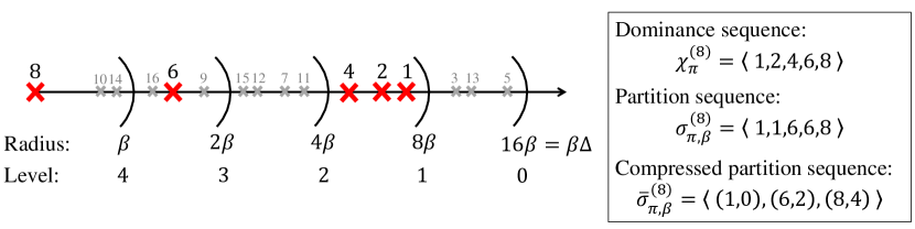
Figure 2: An illustration for dominance sequence, partition sequence and compressed partition sequence for vertex 8. Here we assume that the label of each vertex corresponds to its priority. The left part shows the distances of all vertices to vertex 8 in log-scale, and the red vertices dominate vertex 8.

Proof.

We use the definition of partition sequence and compressed partition sequence from [7]. Given a permutation $\pi$ and a parameter $\beta$, the partition sequence of a point $x\in X$, denoted by $\sigma_{\pi,\beta}^{(x)}$, is the sequence $\displaystyle\sigma_{\pi,\beta}^{(x)}(i)=\min\{\pi(y)\mid y\in X,d(x,y)\leq\beta\cdot 2^{\delta-i}\}$ for $i=0,\ldots,\delta$, i.e. point $y$ has the highest priority among vertices up to level $i$. We note that a trie (radix tree) built on the partition sequence is the FRT tree, but as mentioned we cannot build this explicitly. The compressed partition sequence, denoted as $\bar{\sigma}_{\pi,\beta}^{(x)}$, replaces consecutive equal points in the partition sequence $\sigma_{\pi,\beta}^{(x)}$ by the pair $(p_{i},l_{i})$ where $p_{i}$ is the vertex and $l_{i}$ is the highest level $p_{i}$ dominates $x$ in the FRT tree. Figure 2 gives an example of a partition sequence, a compressed partition sequence, and their relationship to the dominance sequence.

To convert the dominance sequences $\chi_{\pi}$ to the compressed partition sequences $\bar{\sigma}_{\pi,\beta}$ note that for each point $x$ the points in $\bar{\sigma}_{\pi,\beta}^{(x)}$ are a subsequence of $\chi_{\pi}^{(x)}$. Therefore, for $\bar{\sigma}_{\pi,\beta}^{(x)}$, we only keep the highest priority vertex in each level from $\chi_{\pi}^{(x)}$ and tag it with the appropriate level. Since there are only $O(\log n)$ vertices in $\chi_{\pi}^{(x)}$ w.h.p., the time to generate $\bar{\sigma}_{\pi,\beta}^{(x)}$ is $O(\log n)$ w.h.p., and hence the overall construction time is $O(n\log n)$ w.h.p.

The compressed FRT tree can be easily generated from the compressed partition sequences $\bar{\sigma}_{\pi,\beta}$. Blelloch et. al. [7] describe a parallel algorithm that runs in $O(n^{2})$ time (sufficient for their purposes) and polylogarithmic depth. Here we describe a similar version to generate the FRT tree sequentially in $O(n\log n)$ time w.h.p. The idea is to maintain the FRT as a patricia trie [28] (compressed trie) and insert the compressed partition sequences one at a time. Each insertion just needs to follow the path down the tree until it diverges, and then either split an edge and create a new node, or create a new child for an existing node. Note that a hash table is required to trace the tree nodes since the trie has a non-constant alphabet. Each insertion takes time at most the sum of the depth of the tree and the length of the sequence, giving the stated bounds. ∎

We note that for the same permutation $\pi$ and radius parameter $\beta$, it generates exactly the same tree as the original algorithm in [16].

4.3 Expected Stretch Bound

In Section 4.2 we discussed the algorithm to convert the dominance sequences to a FRT tree. When the dominance sequences is generated from a graph metric $(G,d_{G})$, the expected stretch is $O(\log n)$, which is optimal, and the proof is given in many previous papers [16, 7]. Here we show that any distance function $\hat{d}_{G}$ in Lemma 4.3 is sufficient to preserve this expected stretch. As a result, we can use the approximate shortest-paths computed in Section 3 to generate the dominance sequences and further convert to optimal tree embeddings.

Lemma 4.3.

Given a graph metric $(G,d_{G})$ and a distance function $\hat{d}_{G}(u,v)$ such that for $u,v,w\in V$, $\lvert\hat{d}_{G}(u,v)-\hat{d}_{G}(u,w)\rvert\leq 1/\alpha\cdot d_{G}(v,w)$ and $d_{G}(u,v)\leq\hat{d}_{G}(u,v)\leq 1/\alpha\cdot d_{G}(u,v)$ for some constant $0<\alpha\leq 1$, then the dominance sequences based on $(G,\hat{d}_{G})$ can still yield optimal tree embeddings.

Proof outline.

Since the overestimate distances hold the dominating property of the tree embeddings, we show the expected stretch is also not affected. We now show the expected stretch is also held.

Recall the proof of the expected stretch by Blelloch et al. in [7] (Lemma 3.4). By replacing $d_{G}$ by $\hat{d}_{G}$, the rest of the proof remains unchanged except for Claim 3.5, which upper bounds the expected cost of a common ancestor $w$ of $u,v\in V$ in $u$ and $v$’s dominance sequences. The original claim indicates that the probability that $u$ and $v$ diverges in a certain level centered at vertex $w$ is $O(\lvert d_{G}(w,u)-d_{G}(w,v)\rvert/d_{G}(u,w))=O(d_{G}(u,v)/d_{G}(u,w))$ and the penalty is $O(d_{G}(u,w))$, and therefore the contribution of the expected stretch caused by $w$ is the product of the two, which is $O(d_{G}(u,v))$ (since there are at most $O(\log n)$ of such $w$ (Lemma 4.1), the expected stretch is thus $O(\log n)$). With the distance function $\hat{d}_{G}$ and $\alpha$ as a constant, the probability now becomes $O(\lvert\hat{d}_{G}(w,u)-\hat{d}_{G}(w,v)\rvert/\hat{d}_{G}(u,w))=O(d_{G}(u,v)/d_{G}(u,w))$, and the penalty is $O(\hat{d}_{G}(u,w))=O(d_{G}(u,w))$. As a result, the expected stretch asymptotically remains unchanged. ∎

4.4 Efficient construction of approximate dominance sequences

Assume that $\hat{d}_{G}(u,v)$ is computed as $d_{u}(v)$ by the shortest-path algorithm in Section 3 from the source node $u$. Notice that $d_{u}(v)$ does not necessarily to be the same as $d_{v}(u)$, so $(G,\hat{d}_{G}(u,v))$ is not a metric space. Since the computed distances are distance preserving, it is easy to check that Lemma 4.3 is satisfied, which indicate that we can generate optimal tree embeddings based on the distances. This leads to the main theorem of this section.

Theorem 4.4.

(Efficient optimal tree embeddings) There is a randomized algorithm that takes an undirected positively weighted graph $G=(V,E)$ containing $n=|V|$ vertices and $m=|E|$ edges, and produces an tree embedding such that for all $u,v\in V$, $d_{G}(u,v)\leq d_{T}(u,v)$ and $\operatorname{\bf{E}}[d_{T}(u,v)]\leq O(\log n)\cdot d_{G}(u,v)$. The algorithm w.h.p. runs in $O(m\log n)$ time.

The algorithm computes approximate dominance sequences $\hat{\chi}_{\pi}$ by the approximate SSSP algorithm introduced in Section 3. Then we apply Lemma 4.2 to convert $\hat{\chi}_{\pi}$ to an tree embedding. Notice that this tree embedding is an FRT-embedding based on $\hat{d}_{G}$. We still call this an FRT-embedding since the overall framework to generate hierarchical tree structure is similar to that in the original paper [16].

The advantage of our new SSSP algorithm is that the Decrease-Key and Extract-Min operation only takes a constant time when the relative edge range (maximum divided by minimum) is no more than $n^{O(1)}$. Here we adopt the similar idea from [23] to solve the subproblems on specific edge ranges, and concatenate the results into the final output. We hence require a pre-process to restrict the edge range. The pseudocode is provided in Algorithm 3, and the details are explained as follows.

Pre-processing (line 1–3 in Algorithm 3). The goal is to use $O(m\log n)$ time to generate a list of subproblems: the $i$-th subproblem has edge range in the interval $[n^{i-1},n^{i+1}]$ and we compute the elements in the dominance sequences with values falling into the range from $n^{i}$ to $n^{i+1}$. All the edge weights less than the minimum value of this range are treated as 0. Namely, the vertices form some components in one subproblem and the vertex distances within each component is 0. We call this component in a specific subproblem the vertex component. Next we will show: first, how to generate the subproblems; and second, why the computed approximate distances can generate a constant approximation of the original graph metric.

To generate the subproblems, we first sort all edges by weights increasingly, and then use a scan process to partition edges into different ranges. In the pseudocode we first compute the integer part of the logarithm of each edge to based $n$, and then scan the edge list to find the boundaries between different logarithms. Then we have the marks of the beginning edges and ending edges in each subproblem. To compute the logarithms, we use another scan process that computes $n^{i}$ accordingly and compare the weight of each edge to this value. Therefore only two types of operations, comparison and multiplication, are used, which are supported in most of the computational models. This implementation requires edge weights to be no more than $n^{O(m)}$, but if not, we can just add an extra condition in the scan process: if the difference between two consecutive edges in the sorted list is at least $n^{2}$ times, then instead of aligning the boundary of subproblems using powers of $n$, we leave an empty subproblem between these two edges, and and set the left boundary of the next subproblem to be the larger edge weight. Since we do not actually use the exact values of the logarithms other than determining the boundaries between subproblems, this change will not affect following computations but bound the amount of subproblems. This step takes $O(m\log n)$ work.

Since in the subproblems zero-weight edges form vertex components, we need to keep a data structure to maintain the vertex components in all levels such that: given any specific subproblem, (1) the vertex component containing any vertex $v$ can be found in $O(\log n)$ time; and (2) the all vertices in a component can be acquired with the cost linear to the number of vertices in this component. This data structure is implemented by union-find (tree-based with no path compressions) and requires an extra scanning process as preprocessing. This preprocessing is similar to run Kruskal’s algorithm [24] to compute minimum spanning trees. We construct this data structure using a scan on the edges in an increasing order of edge weights. For each edge, if it merges two components, we merge the two trees in union-find by rank, add two directed edges between the roots, and update the root’s priority if the component with smaller rank has a higher priority. Meanwhile the newly added edges also store the loop variable $i$ (line 3). The vertices in a component in the $i$-th subproblem (line 3) can be found by traversing from any vertex in the final union-find tree, but ignoring the edges with the stored loop variables larger than $i$. Finally, given a vertex and a subproblem, the components can be queried by traversing to the root in the union-find tree until reaching the vertex root of this vertex component, and the cost is $O(\log n)$ per query. The cost of this step is also $O(m\log n)$.

Computing approximate dominance sequences (line 3 – line 3). After preprocessing, we run the shortest-path algorithm on each subproblem, and the $i$-th subproblem generates the entries in the approximate dominance sequences in the range of $[n^{i},n^{i+1})$. The search is restricted to edges with weights less than $n^{i+1}$. Meanwhile the lengths of edges less than $n^{i-1}$ are treated as zero, and the vertices with zero distances can be queried with the union-find tree computed in the preprocessing. Finally, we solve an extra subproblem that only contains edges with weight less than $n$ to generate the elements in dominance sequences in $[1,n)$.

Observe that in the $i$-th subproblem, if vertex $v$ dominates vertex $u$ with distance at least $n^{i}$, then (1) $v$ dominates all vertices in the vertex component containing $u$; (2) $v$ has the highest priority in $v$’s vertex component. We thus can apply the approximate shortest-path described in Section 3.1 with simple modifications to compute the dominance sequences. For each vertex component, we only run the shortest-path from the highest priority vertex, whose label is stored in the root node in the union-find tree. When it dominates another vertex component, then we try to append this vertex to the dominance sequence of each vertex in the component. This process is shown as the function ComputeDistance in Algorithm 3.

Correctness and tree properties. Lemma 4.3 indicates that optimal tree embeddings can be constructed based on $\hat{d}_{G}(u,v)$ as long as $\hat{d}_{G}(u,v)$ is computed as $d_{u}(v)$ by the any single-source shortest-path algorithm that is $\alpha$-distance preserving for any constant $\alpha$. We now show that the output of Algorithm 3, approximate dominance sequences $\hat{\chi}_{\pi}$, is such $\hat{d}_{G}(u,v)$ with $\alpha=1/8$.

Theorem 3.1 shows that the computed distances of SSSP algorithm is $1/4$-distance preserving. Furthermore, the partitioning of the computation into multiple subproblems also leads to an approximation. The worst approximation lies in the case of a path containing $n-2$ edges with length $n^{i}-\epsilon$ (for an arbitrary small $\epsilon>0$) and one edge with length $n^{i+1}$. In this case the approximated distance is $n^{i+1}$, and the actual distance is no more than $(2n-2)n^{i}$, so the gap is at most a factor of 2. Clearly this approximation satisfies $\lvert\hat{d}_{G}(u,v)-\hat{d}_{G}(u,w)\rvert\leq 1/\alpha\cdot d_{G}(v,w)$. Combining these two together gives the stated results.

We also need to show that for a pair of vertices $u,v\in V$ and the permutation $\pi$, if $u$ dominates $v$ in $\hat{d}_{G}$, the algorithm will add $u$ to ${\hat{\chi}_{\pi}}^{(v)}$. Assume $\hat{d}_{G}(u,v)\in[n^{i},n^{i+1})$, then $u$ dominates $v$ in $\hat{d}_{G}$ iff $u$ has the highest priority for the vertex component in the $i$-th subproblem and dominates the vertex component containing $v$. Then Algorithm 3 will correctly add $u$ in ${\hat{\chi}_{\pi}}^{(v)}$.

Time complexity. Finally we show that Algorithm 3 has time complexity $O(m\log n)$ w.h.p. This indicates that the whole construction process costs $O(m\log n)$, since the postprocessing to construction of an FRT tree based on dominance sequences has cost $O(n\log n)$ w.h.p. We have shown that the pre-processing has time complexity $O(m\log n)$. The remaining parts include the search for approximate shortest paths, and the construction of the approximate dominance sequences.

We first analyze the cost of shortest-path searches. For each subproblem, Lemma 2.1 shows that w.h.p. at most $O(\log n)$ vertex components dominate a specific vertex component. Hence the overall operation number of Decrease-Key and Extract-Min is $O(m^{\prime}\log n)$ where $m^{\prime}$ is the number of edges in this subproblem. Since each edge is related to at most two subproblems, the overall cost of shortest-path search is $O(m\log n)$ w.h.p.

Next we provide the analysis of the construction of dominance sequences. We have shown that Algorithm 3 actually computes the dominance sequences of an approximate graph metric, so the overall number of elements in $\hat{\chi}_{\pi}$ is $O(n\log n)$ w.h.p. Since the vertex components can be retrieved using the union-find structure, the cost to find each vertex is $O(1)$ asymptotically. Note that in the $i$-th subproblem, if $\hat{d}_{G}(u,v)\geq n^{i}$, $u$ dominates $v$ if and only if $u$ dominates all vertices in $v$’s component. Therefore $u$ is added to all ${\hat{\chi}_{\pi}}^{(v^{\prime})}$ for $v^{\prime}$ in this component. Since the subproblems are processed in decreasing order on distances (line 3), there will be no multiple insertions for a vertex in an approximate dominance sequence, nor further removal for an inserted element in the sequence. Lemma 4.1 bounds the total number of vertices in all components $S$ by $O(n\log n)$ w.h.p. and each insertion takes $O(1)$ time, so the overall cost to maintain the approximate dominance sequences is $O(n\log n)$ w.h.p. In total, the overall time complexity to construct the approximate dominance sequences is $O(m\log n)$ w.h.p.

Input: A weighted graph $G=(V,E)$ and a random permutation $\pi$.

Output: Approximate dominance sequences $\chi^{\prime}_{\pi}$ and the set of associated distances $d$.

1 Initialize each vertex as a singleton component, i.e. $f(v)\leftarrow v$

2 Sort all edges based on their weights so that $d(e_{1})\leq d(e_{2})\leq\cdots\leq d(e_{m})$

3 $d\leftarrow\varnothing$

4 Computer the logarithm of each edge: ${\mbox{\emph{lg}}}{}_{i}\leftarrow\lfloor\log_{n}{d(e_{i})}\rfloor$

5 Let ${\mbox{\emph{start}}}{}_{i}$ be the first edge that ${\mbox{\emph{lg}}}{}_{i}=i$

6 for $i\leftarrow 0$ to $\lfloor\log_{n}{d(e_{m})}\rfloor$ do

7       for $j\leftarrow{\mbox{\emph{start}}}{}_{i}$ to ${\mbox{\emph{start}}}{}_{i+2}-1$ do

8             Mark the corresponding components for edge $e_{j}$

9      for $j\leftarrow{\mbox{\emph{start}}}{}_{i}$ to ${\mbox{\emph{start}}}{}_{i+1}-1$ do

10             if $e_{j}$ connects two different components then

11                   Merge the smaller component into the larger one

12                   The new component has the priority to be the higher among the previous two

13                  

14 for $i\leftarrow\lfloor\log_{n}{d(e_{m})}\rfloor$ downto 0 do

15       ComputeDistance$(\{e_{{\scriptsize{\mbox{\emph{start}}}{}}_{i}},\cdots,e_{{\scriptsize{\mbox{\emph{start}}}{}}_{i+2}-1}\},d(e_{{\scriptsize{\mbox{\emph{start}}}{}}_{i+1}}))$

16      

17ComputeDistance$(\{e_{1},\cdots,e_{i-1}\},1)$

18 return $\hat{\chi}_{\pi}$, $d$

19 Function ComputeDistance(edgeset $E^{\prime}$, range $r$)

20       Let $C$ be the set of vertex components that contains the endpoints associated to $E^{\prime}$

21       Sort the components based on the priority, i.e. $\pi(V^{\prime}_{1})<\cdots<\pi(V^{\prime}_{|C|})$ for all $V^{\prime}_{i}\in C$

22       Build adjacency list by sort the edges $E^{\prime}$ based on the component endpoints

23       foreach $V^{\prime}\in C$ do  $\delta(V^{\prime})\leftarrow+\infty$

24       for $i\leftarrow 1$ to $|C|$ do

25             Let $p$ be the vertex with the highest priority in $V^{\prime}_{i}$

26             Apply approximate SSSP algorithm to compute $S=\{S^{\prime}\in C\mid d(p,S^{\prime})<\delta(S^{\prime})\}$

27             for $S^{\prime}\in S$ do

28                   $\delta(S^{\prime})\leftarrow d(p,S^{\prime})$

29                   if $\delta(S^{\prime})>r$ then

30                         for $u^{\prime}\in S^{\prime}$ do

31                               Try to append $p$ to ${\hat{\chi}_{\pi}}^{(u^{\prime})}$

32                               If successful, $d\leftarrow d\cup\{(u^{\prime},p)\rightarrow 8\cdot\delta(S^{\prime})\}$

return $\hat{\chi}_{\pi}$, $d$

Algorithm 3 Construction of the approximate dominance sequences

5 Asymptotically Tight Ramsey Partitions Based on FRT Trees

In this section we show that the probability distribution over FRT trees is an asymptotically tight Ramsey Partition. Therefore, FRT trees can be used to construct approximate distance oracle with size $O(n^{1+1/k})$, $O(k)$ stretch and $O(1)$ query time using the algorithm presented in [25]. The construction time of this oracle is $O(n^{1/k}(m\log n+n\log^{2}n))$, which is not only faster than the best known algorithm [26] with $O(n^{1/k}m\log^{3}n)$ time complexity for construction, but also much simpler. More importantly, our new algorithm provides an $18.5k$-approximation, smaller than the bounds $128k$ in [25] and $33k$ in [29].

Recall the definition of Ramsey partitions: given a metric space $(X,d_{X})$, an $(\alpha,\gamma)$ Ramsey partition is the probability distribution over partition trees $\{\mathcal{P}_{k}\}_{k=0}^{\infty}$ of $X$, such that:

$$\Pr\mathopen{}\mathclose{{}\left[\forall i\in\mathbb{N},B_{X}\mathopen{}\mathclose{{}\left(x,\alpha\cdot c^{-i}\Delta}\right)\subseteq\mathcal{P}_{i}(x)}\right]\geq|X|^{-\gamma}.$$

Theorem 5.1.

The probability distribution over FRT trees is an asymptotically tight Ramsey Partition with $\alpha=\Omega(\gamma)$ (shown in the appendix) and fixed $c=2$. More precisely, for every $x\in X$,

$$\Pr\mathopen{}\mathclose{{}\left[\forall i\in\mathbb{N},B_{X}\mathopen{}\mathclose{{}\left(x,\mathopen{}\mathclose{{}\left(1-2^{-1/2a}}\right){2^{-i}\Delta}}\right)\subseteq\mathcal{P}_{i}(x)}\right]\geq{1\over 2}|X|^{-{2\over a}}$$

for any positive integer $a>1$.

Note that the $1/2$ on the right side of the inequality only leads a doubling of the overall trees needed for the Ramsey-based ADO, but does not affect asymptotic bounds.

To prove Theorem 5.1, we first prove some required lemmas.

Lemma 5.2.

Given $n-1$ arbitrarily chosen integers $v_{1},v_{2},\cdots,v_{n-1}$ in $[a]$ ($a\geq 2$), let $S$ be a set in which each $v_{i}$ is selected independently at random with probability $p_{i}\leq{1/(i+1)}$. Given an integer $v$ chosen uniformly at random from $[a]$, we have that

$$\Pr\mathopen{}\mathclose{{}\left[\{s=v:s\in S\}=\varnothing}\right]\geq{\epsilon}\cdot n^{-1/(a(1-\epsilon))}$$

for any $\epsilon\in[a-1]/a$.

Proof.

Construct $a$ buckets so that each value is in the $v_{i}$-th bucket. Let $s_{j}=\ln\prod_{v_{i}\in{\rm{bucket}}_{j}}(1-p_{i})=\sum_{v_{i}\in{\rm{bucket}_{j}}}\ln(1-p_{i})$. With the fact that $\prod_{i=2}^{n}(1-1/i)=1/n$, we have $\sum_{j=1}^{a}s_{j}=\sum_{i=1}^{n}\ln(1-p_{i})\geq\sum_{i=1}^{n-1}\ln(i/(i+1))=-\ln n$. Therefore, there exists at least $\epsilon a$ buckets such that their $s_{j}$ are at least $-1/(a(1-\epsilon))\cdot\ln n$. For these buckets, the probability that none of the points in a specific bucket are selected is $\prod_{v_{i}\in{\rm{bucket}_{j}}}(1-p_{i})=e^{s_{j}}\geq n^{-1/(a(1-\epsilon))}$. Hence the probability that a randomly chosen bucket is empty is at least $\epsilon\cdot n^{-1/(a(1-\epsilon))}$. ∎

Lemma 5.3.

Given $n-1$ points $v_{1},v_{2},\cdots,v_{n-1}$ in $[0,1)$, select each independently with probability $p_{i}\leq{1/(i+1)}$. For a uniformly randomly-picked $b$ in $[0,1)$, the probability that no point $v_{i}$ in the range $[b-1/2a,b+1/2a)\,\operatorname{mod}\,1$ is selected is at least ${\epsilon}\cdot n^{-1/(a(1-\epsilon))}$ for any positive integer $a\geq 2$ and $\epsilon\in[a-1]/a$.

Proof.

Given $b$, we construct $a$ buckets where the $i$-th bucket contains the points that fall into the range $[b+(i-1/2)/a,b+(i+1/2)/a)\,\operatorname{mod}\,1$. Since any $b^{\prime}=(b+i/a)\,\operatorname{mod}\,1~{}(i\in[a])$ will create the same buckets and $b$ is uniformly distributed in $[0,1)$, by applying Lemma 5.2, the probability that a chosen bucket is empty is at least ${\epsilon}\cdot n^{-1/(a(1-\epsilon))}$ on average. ∎

In Lemma 5.3, $b$ will be related to $\beta$ in the FRT tree, and $a$ will represent the padded ratio in Theorem 5.1.

Proof of Theorem 5.1.

In this proof, we focus on one specific element $x\in X$.

Let $d_{1},d_{2},\cdots,d_{|X|-1}$ be the distances from $x$ to all the other elements. We transform these distances to the log-scale and ignore the integer parts by denoting $\delta(d_{i})=(\log_{2}d_{i})\,\operatorname{mod}\,1$. Therefore, the radii of the hierarchical partitions $\{\beta\Delta,\beta\Delta/2,\beta\Delta/4,\dots\}$ will be exactly the same as $\beta^{\prime}=\log_{2}(\beta\Delta)\,\operatorname{mod}\,1=\log_{2}\beta$ after this transformation, and $\beta^{\prime}$ follows the uniform distribution on $[0,1]$ according to the FRT algorithm.

WLOG, assume the distances are in increasing order, i.e. $0<d_{1}\leq d_{2}\leq\cdots\leq d_{|X|-1}$. Due to the property of a random permutation, the probability for each element to be in the dominance sequence of $x$ is $p_{1}={1\over 2},p_{2}={1\over 3},\cdots,p_{n-1}={1\over n}$.

Now we compute the probability that none of the distances from $x$ to the elements in the dominance sequence of $x$ are in the padded region near the boundary. The radii of the partitions are $2^{-i}\beta\Delta$, so the padded region stated in Theorem 5.1 is $\bigcup_{i=0}^{+\infty}\mathopen{}\mathclose{{}\left[\mathopen{}\mathclose{{}\left(1-\mathopen{}\mathclose{{}\left(1-2^{-1/2a}}\right)}\right)\cdot 2^{-i}\beta\Delta,\mathopen{}\mathclose{{}\left(1+\mathopen{}\mathclose{{}\left(1-2^{-1/2a}}\right)}\right)\cdot 2^{-i}\beta\Delta}\right]$. These intervals after transformation are all in $[\beta^{\prime}-1/2a,\beta^{\prime}+1/2a)\,\operatorname{mod}\,1$. The probability that none of the elements in the interval $[\beta^{\prime}-1/2a,\beta^{\prime}+1/2a)\,\operatorname{mod}\,1$ is in the dominance sequence of $x$, is equivalent to elements not being selected in the range in Lemma 5.3. This gives a probability of at least ${1\over 2}|X|^{-{2/a}}$ if $\epsilon$ is set to be $1/2$ (or $\epsilon=(a-1)/2a$ for odd integer $a$).

Since all of $x$’s ancestors are in the dominance sequence of $x$, the probability that none of them are in that padded range is also at least ${1\over 2}|X|^{-{2/a}}$. ∎

Remark 1.

There are two major differences between this construction (based on FRT trees) and the original construction in [25] (based on hierarchical CKR partitions). First, there is only one random permutation for all levels in one FRT tree, but the hierarchical CKR partitions requires different random permutations in different levels. Second, the radii for the partitions decrease exactly by a half between two consecutive levels in FRT trees, but the radii in hierarchical CKR partitions is randomly generated in every level.

Theorem 5.1 shows that the extra randomness to generate multiple random permutation and radii is unnecessary to construct Ramsey partitions. Moreover, since the radii for the partitions decrease by a half between two consecutive levels (instead of at most 16 in the original construction), the stretch can be reduced to $18.5k$ as opposed to $128k$, which is shown in appendix D. Lastly, the proof is also very different and arguably simpler.

Corollary 5.4.

With Theorem 5.1, we can accelerate the time to construct the Ramsey-partitions-based Approximate Distance Oracle in [25] to

$$O\mathopen{}\mathclose{{}\left(n^{1/k}(m+n\log n)\log n}\right)$$

on a graph with $n$ vertices and $m$ edges, improving the stretch to $18.5k$, while maintaining the same storage space and constant query time.

This can be achieved by replacing the original hierarchical partition trees in the distance oracles by FRT trees (and some other trivial changes). The construction time can further reduce to $O\mathopen{}\mathclose{{}\left(n^{1/k}m\log n}\right)$ using the algorithm introduced in Section 4.4 while the oracle still has a constant stretch factor. Accordingly, the complexity to construct Christian Wulff-Nilsen’s Distance Oracles [35] and Shiri Chechik’s Distance Oracles [9] can be reduced to

$$O\mathopen{}\mathclose{{}\left(kmn^{1/k}+kn^{1+1/k}\log n+n^{1/ck}m\log n}\right)$$

since they all use Mendel and Naor’s Distance Oracle to obtain an initial distance estimation. The acceleration is from two places: first, the FRT tree construction is faster; second, FRT trees provide better approximation bound, so the $c$ in the exponent becomes smaller.

6 Conclusion

In this paper we described a simple and efficient algorithm to construct FRT embeddings on graphs using $O(m\log n)$ time, which is based on a novel linear-time algorithm for single-source shortest-paths proposed in this paper. We also studied the distance preserving properties on FRT embeddings, and proved that FRT trees are asymptotic optimal Ramsey partitions. Lastly, we used the FRT trees to construct a simple and programming-friendly distance oracle, which surprisingly shows good approximation on all of our testing cases.

Appendix A Proof for Lemma 4.1

Proof of Lemma 4.1.

For a fixed point $x\in X$, we first sort all of the vertices by their distances to $x$, and hence $0=d(x,x_{1}^{\prime}=x)<d(x,x_{2}^{\prime})\leq d(x,x_{3}^{\prime})\leq\cdots\leq d(x,x_{n}^{\prime})$. Let $y_{i}=\min\{\pi(x_{j}^{\prime})\,|\,j\leq i\}$. By definition, $x_{i}^{\prime}$ is in the dominance sequence of $x$ if and only if $\pi(x_{i}^{\prime})<\pi(x_{j}^{\prime})$ for all $j<i$, which is also equivalent to $y_{i}<y_{i-1}$ for $i>1$. Thus, $\mathopen{}\mathclose{{}\left|\chi_{\pi}^{(x)}}\right|$ is the number of different elements in $y_{i},1\leq i\leq n$. Since $\pi$ is a random permutation and independent to the distances to $x$, by applying Lemma 2.1, there exist $O(\log n)$ elements in $\chi_{\pi}^{(x)}$ w.h.p.

Therefore, the total elements in dominance sequences of $G$ are $O(n\log n)$ w.h.p. simply by summing up dominance sequences for all vertices. ∎

Appendix B Dominance Sequence Construction based on Dijkstra’s Algorithm

Input: A weighted graph $G=(V,E)$ and a random permutation $\pi$.

Output: Dominance Sequences $\chi_{\pi}$ and the set of associated distances $d$.

1 foreach $v\in V$ do  $\delta(v)\leftarrow+\infty$

2 $d\leftarrow\varnothing$

3 for $i\leftarrow 1$ to $|V|$ do

4       $u\leftarrow\pi^{-1}(i)$

5       $Q\leftarrow\{u\}$

6       $\delta(u)\leftarrow 0$

7       while $Q\neq\varnothing$ do

8             Extract $v\in Q$ with minimal $\delta(v)$

9             $\chi_{\pi}^{(v)}\leftarrow\chi_{\pi}^{(v)}+u$    // add $u$ to $v$’s dominance sequence

10             $d\leftarrow d\cup\{(u,v)\rightarrow\delta(v)\}$

11             foreach $w:(v,w,l_{v,w})\in E$ do

12                   if $\delta(w)>\delta(v)+l_{v,w}$  then

13                         $\delta(w)\leftarrow\delta(v)+l_{v,w}$    // $l_{v,w}$ is the edge length

14                         $Q\leftarrow Q\cup\{w\}$

15                        

return $\chi_{\pi}$, $d$

Algorithm 4 The dominance sequences construction

Here we review the algorithm proposed by Cohen [11] to compute dominance sequence, which is basically a variation of Dijkstra’s algorithm. The dominance sequences $\chi_{\pi}$ can be trivially constructed by running SSSP from each vertex, but this takes $O(n(m+n\log n))$ time. An important observation is that: for each vertex $u$, if its distance to another vertex $v$ is larger than $v$’s distance to a higher priority vertex $\bar{u}$, then it is not necessary to explore $v$ when running the SSSP from $u$. This is because $\bar{u}$ is closer to $v$ and has a higher priority. Similar ideas can be found in related works [34, 26].

Inspired by this observation, we run Dijkstra algorithm with the source vertices in increasing order in $\pi$, but for each source vertex $u$, we only explore the vertices that are closer to $u$ than any other previous source vertices. The algorithm first starts the SSSP from $\pi^{-1}(1)$ and adds this vertex to the dominance sequence of all vertices, then it starts the SSSP from $\pi^{-1}(2)$ but only adds it to the dominance sequence of the vertices that are closer to $\pi^{-1}(2)$ than $\pi^{-1}(1)$, and this repeats for $n$ times. In the algorithm, $\delta(u)$ in the $i$-th round is the shortest distance of $u$ to any of the first $i$ vertices, so that the SSSP is restricted in each round to vertices for which $\delta(u)$ is updated. Since $\delta(u)$ is not initialized in each round, the overall time complexity is largely decreased.

Lemma B.1.

Given a graph metric $(X,d_{X})$ and a random permutation $\pi$, the dominance sequences $\chi_{\pi}$ can be constructed in $O(m\log n+n\log^{2}n)$ time w.h.p.

Proof.

Lemma 4.1 indicates that w.h.p. the total number of delete-min operations (line 4) is $|\chi_{\pi}|=O(n\log n)$ and the overall number of decrease-key operations (line 4) is $\sum_{u}\deg(u)\cdot\mathopen{}\mathclose{{}\left|\chi_{\pi}^{(u)}}\right|=O(m\log n)$. Thus, if the priority queue $Q$ in Algorithm 4 is implemented using Fibonacci heap, the overall time complexity for Algorithm 4 is $O(m\log n+n\log^{2}n)$ w.h.p. ∎

Lastly, we show the correctness of the dominance sequences construction algorithm.

Lemma B.2.

Given the random permutation $\pi$, and the graph $G=(V,E)$, the dominance sequence of a specific vertex $v\in V$ will be stored in $\chi_{\pi}^{(v)}$ at the end of Algorithm 4, and consequently the distances between every vertex and its dominating vertices are in $d$.

Proof.

First we prove that all vertices that dominate $v$ are in $\chi_{\pi}^{(v)}$.

Assuming that $u\in V$ is a vertex and dominates $v$, we show that $u\in\chi_{\pi}^{(v)}$. Let $(w_{1}=u,w_{2},\dots,w_{k-1},w_{k}=v)$ be the shortest path from $u$ to $v$. Since $u$ dominates $v$, $\pi(u)<\pi(w_{i})$ holds for all $i=2,3,\dots,k$.

We first prove that $u$ dominates all the vertices on the shortest path. Assume to the contrary that there exists at least one vertex $w_{i}$ that is not dominated by $u$, which means that at least another vertex $u^{*}$ holds both $\pi(u^{*})<\pi(u)$ and $d(u^{*},w_{i})\leq d(u,w_{i})$. This indicates that the distance from $u^{*}$ to $v$ is at most $d(u^{*},w_{i})+\sum_{j=i}^{k-1}d(w_{j},w_{j+1})\leq\sum_{j=1}^{k-1}d(w_{j},w_{j+1})=d(u,v)$. Combining with the other assumption $\pi(u^{*})<\pi(u)$, it directly leads to a contradiction that $u^{*}$ dominates $v$, since $u^{*}$ is closer to $v$ and owns a higher priority.

Then we prove that when the outermost for-loop is at vertex $u$, vertex $v$ will be extracted (in line 4) from $Q$. Then $u$ will be added into $\chi_{\pi}^{(v)}$ and $\delta(v)$ will be updated by $d(u,v)$ by induction. Initially $w_{1}=u$ is added to $\chi_{\pi}^{(w_{1})}$ (and changes $\delta(w_{1})$ to be $d(u,u)=0$), which is the base case. On the inductive step, we show that as long as $u$ is attached to $\chi_{\pi}^{(w_{i-1})}$ in line 4, all $w_{i}$ will be inserted into $Q$ later in line 4, and finally $u$ will be added to $\chi_{\pi}^{(w_{i})}$. From the previous conclusion, we know that $u$ dominates $w_{i}$ via the shortest path $(w_{1},w_{2},\dots,w_{i})$, so that $\delta(w_{i})>d(u,w_{i-1})+d(w_{i-1},w_{i})=\delta(w_{i-1})+d(w_{i-1},w_{i})$, which guarantees that the checking in line 4 for edge $(w_{i},w_{i+1})$ will be successful. After that, $w_{i}$ will be inserted into $Q$ and $u$ will be attached to $\chi_{\pi}^{(v)}$ later, and $\delta(w_{i})$ will be updated to $d(u,w_{i-1})+c_{w_{i-1},w_{i}}$, which is the new $d(u,w_{i})$.

We now show that all vertices in $\chi_{\pi}^{(v)}$ dominate $v$. Assume to the contrary that at the end of the algorithm, $\exists u\in\chi_{\pi}^{(v)}$ and $u$ does not dominate $v$. This means there exists $u^{*}$ which satisfies both prior to $u$ and $d(v,u^{*})<d(v,u)$. From $\pi(u^{*})<\pi(u)$ we know that when the outmost for-loop is at $u$, $u^{*}$ has already been proceeded so $\delta(v)\leq d(v,u^{*})<d(v,u)$. Consider when $v$ is added to $Q$, we have $\delta(v)>\delta(u^{\prime})+c_{v,u^{\prime}}=d(u,u^{\prime})+c_{v,u^{\prime}}\geq d(v,u)$, which contradicts to $\delta(v)<d(v,u)$.

Lastly, since line 9 and line 10 are always executed together, once a vertex is added to the dominance sequence of another vertex, the corresponding pairwise distance is added to $d$, and the distance is guaranteed to be the shortest by the correctness of Dijkstra’s algorithm.

Also, since $\delta(v)$ is always decreasing during the algorithm, the dominant vertices are added to $\chi_{\pi}^{(v)}$ in decreasing order of their distance to $v$. ∎

Appendix C Asymptotic Tight Bound of Ramsey partition in Theorem 5.1

In case of any unclear, here we show that in Theorem 5.1, $\alpha=\mathopen{}\mathclose{{}\left(1-2^{-1/2a}}\right)=\Omega(\gamma)$.

Proof.

Let $f(t)=2^{-t}+\frac{1}{2}t$, then $\frac{\mathrm{d}f}{\mathrm{d}t}=-2^{-t}\ln 2+\frac{1}{2}$.

For any $t$ that $0<t\leq\frac{1}{4}$, we have $-2^{-t}\ln 2+\frac{1}{2}<-2^{-1/4}\ln 2+\frac{1}{2}<0$, which shows that $f$ monotonously decreases in range $\mathopen{}\mathclose{{}\left(0,\frac{1}{4}}\right]$. Thus,

$$f(t)<f(0)=1$$ (1)

for $0<t\leq\frac{1}{4}$.

Any integer $a$ that $a\geq 2$ leads to $0<\frac{1}{2a}\leq\frac{1}{4}$. Plugging $t=\frac{1}{2a}$ in (1), we get $f(\frac{1}{2a})=2^{-1/2a}+\frac{1}{4a}<1$, which further shows that $1-2^{-1/2a}>\frac{1}{2}\cdot\frac{1}{2a}=\Omega(\frac{1}{2a})$. ∎

Appendix D Approximation Factor for Theorem 5.1

For any fix integer $a>1$, we now try to analyze a pair of vertices $u$ and $v$ in graph $G$. Let $u$ be the first padded point in the pair in the $t$-th FRT tree, which means that $u$ is “far away” from the boundaries of the hierarchical partitioning in that tree. Assume that the lowest common ancestor of the vertices be in the $i$-th level in the $t$-th FRT tree. Since $u$ is padded, the distance $d_{G}(u,v)$ is at least $\mathopen{}\mathclose{{}\left(1-2^{-1/2a}}\right)\cdot{2^{-i-1}\beta\Delta}$. The distance reported from the tree query $d_{T}(u,v)$ is no more than $2\cdot 2^{-i}\beta\Delta$. Therefore, $d_{G}(u,v)\geq\mathopen{}\mathclose{{}\left(1-2^{-1/2a}}\right)/4\cdot d_{T}(u,v)$.

Storing this data structure requires expected $O\mathopen{}\mathclose{{}\left({1/\epsilon}\cdot n^{1+1/(a(1-\epsilon))}}\right)$ space. Notice that any $a\leq 2$ does not make sense since storing the distances for the whole matric space need $O(n^{2})$ space. For any $a>2$, let $\epsilon=\lfloor a/3\rfloor/a$, so distance oracle in Theorem 5.1 using $O\mathopen{}\mathclose{{}\left(n^{1+1/k}}\right)$ space (integer $k=a-\lfloor a/3\rfloor$) provided $18.5k$ distance approximation (achieved maximum $18.33k$ when $a=3$).

References

- [1] Rachit Agarwal and Philip Godfrey. Distance oracles for stretch less than 2. In Proceedings of ACM-SIAM Symposium on Discrete Algorithms (SODA), pages 526–538, 2013.
- [2] Noga Alon, Richard M Karp, David Peleg, and Douglas West. A graph-theoretic game and its application to the k-server problem. SIAM Journal on Computing, 24(1):78–100, 1995.
- [3] Yair Bartal. Probabilistic approximation of metric spaces and its algorithmic applications. In In Proceedings of IEEE Foundations of Computer Science (FOCS), pages 184–193, 1996.
- [4] Yair Bartal. On approximating arbitrary metrices by tree metrics. In Proceedings of ACM Symposium on Theory of Computing (STOC), pages 161–168. ACM, 1998.
- [5] Surender Baswana and Telikepalli Kavitha. Faster algorithms for approximate distance oracles and all-pairs small stretch paths. In In Proceedings of IEEE Symposium on Foundations of Computer Science (FOCS), pages 591–602, 2006.
- [6] Guy E Blelloch, Yan Gu, Julian Shun, and Yihan Sun. Parallelism in randomized incremental algorithms. In In Proceedings of ACM Symposium on Parallelism in Algorithms and Architectures (SPAA), pages 467–478, 2016.
- [7] Guy E Blelloch, Anupam Gupta, and Kanat Tangwongsan. Parallel probabilistic tree embeddings, k-median, and buy-at-bulk network design. In In Proceedings of ACM symposium on Parallelism in Algorithms and Architectures (SPAA), pages 205–213, 2012.
- [8] Gruia Calinescu, Howard Karloff, and Yuval Rabani. Approximation algorithms for the 0-extension problem. SIAM Journal on Computing, 34(2):358–372, 2005.
- [9] Shiri Chechik. Approximate distance oracles with constant query time. In In Proceedings of ACM Symposium on Theory of Computing (STOC), pages 654–663, 2014.
- [10] Shiri Chechik. Approximate distance oracles with improved bounds. In In Proceedings of ACM on Symposium on Theory of Computing (STOC), pages 1–10, 2015.
- [11] Edith Cohen. Size-estimation framework with applications to transitive closure and reachability. Journal of Computer and System Sciences, 55(3):441–453, 1997.
- [12] Edith Cohen. Polylog-time and near-linear work approximation scheme for undirected shortest paths. Journal of the ACM (JACM), 47(1):132–166, 2000.
- [13] Michael B. Cohen, Rasmus Kyng, Gary L. Miller, Jakub W. Pachocki, Richard Peng, Anup B. Rao, and Shen Chen Xu. Solving SDD linear systems in nearly time. In Proceedings of ACM Symposium on Theory of Computing (STOC), pages 343–352, 2014.
- [14] Edsger W Dijkstra. A note on two problems in connexion with graphs. Numerische mathematik, 1(1):269–271, 1959.
- [15] Michael Elkin and Seth Pettie. A linear-size logarithmic stretch path-reporting distance oracle for general graphs. In Proceedings of ACM-SIAM Symposium on Discrete Algorithms (SODA), pages 805–821, 2015.
- [16] Jittat Fakcharoenphol, Satish Rao, and Kunal Talwar. A tight bound on approximating arbitrary metrics by tree metrics. Journal of Computer and System Sciences (JCSS), 69(3):485–497, 2004.
- [17] Michael L Fredman and Robert Endre Tarjan. Fibonacci heaps and their uses in improved network optimization algorithms. Journal of the ACM (JACM), 34(3):596–615, 1987.
- [18] Stephan Friedrichs and Christoph Lenzen. Parallel metric tree embedding based on an algebraic view on moore-bellman-ford. In Proceedings of ACM Symposium on Parallelism in Algorithms and Architectures (SPAA), pages 455–466, 2016.
- [19] Harold N Gabow. Scaling algorithms for network problems. Journal of Computer and System Sciences, 31(2):148–168, 1985.
- [20] Mohsen Ghaffari and Christoph Lenzen. Near-optimal distributed tree embedding. In International Symposium on Distributed Computing, pages 197–211. Springer, 2014.
- [21] David R Karger and Matthias Ruhl. Finding nearest neighbors in growth-restricted metrics. In In Proceedings of ACM symposium on Theory of Computing (STOC), pages 741–750. ACM, 2002.
- [22] Maleq Khan, Fabian Kuhn, Dahlia Malkhi, Gopal Pandurangan, and Kunal Talwar. Efficient distributed approximation algorithms via probabilistic tree embeddings. Distributed Computing, 25(3):189–205, 2012.
- [23] Philip N Klein and Sairam Subramanian. A randomized parallel algorithm for single-source shortest paths. Journal of Algorithms, 25(2):205–220, 1997.
- [24] Joseph B Kruskal. On the shortest spanning subtree of a graph and the traveling salesman problem. Proceedings of the American Mathematical society, 7(1):48–50, 1956.
- [25] Manor Mendel and Assaf Naor. Ramsey partitions and proximity data structures. In In Proceedings of IEEE Symposium on Foundations of Computer Science (FOCS), pages 109–118, 2006.
- [26] Manor Mendel and Chaya Schwob. Fast CKR partitions of sparse graphs. Chicago Journal of Theoretical Computer Science, (2):1–18, 2009.
- [27] Gary L. Miller, Richard Peng, Adrian Vladu, and Shen Chen Xu. Improved parallel algorithms for spanners and hopsets. In In Proceedings of ACM Symposium on Parallelism in Algorithms and Architectures (SPAA), pages 192–201.
- [28] Donald R. Morrison. Patricia—practical algorithm to retrieve information coded in alphanumeric. Journal of the ACM (JACM), 15(4):514–534, October 1968.
- [29] Assaf Naor and Terence Tao. Scale-oblivious metric fragmentation and the nonlinear Dvoretzky theorem. Israel Journal of Mathematics, 192(1):489–504, 2012.
- [30] Seth Pettie and Vijaya Ramachandran. A shortest path algorithm for real-weighted undirected graphs. SIAM J. Comput., 34(6):1398–1431, 2005.
- [31] Harald Räcke. Optimal hierarchical decompositions for congestion minimization in networks. In Proceedings of ACM Symposium on Theory of Computing (STOC), pages 255–264, 2008.
- [32] Raimund Seidel. Backwards analysis of randomized geometric algorithms. Springer, 1993.
- [33] Mikkel Thorup. Undirected single source shortest paths in linear time. In In Proceedings of IEEE Symposium on Foundations of Computer Science (FOCS), pages 12–21, 1997.
- [34] Mikkel Thorup and Uri Zwick. Approximate distance oracles. Journal of the ACM (JACM), 52(1):1–24, 2005.
- [35] Christian Wulff-Nilsen. Approximate distance oracles with improved query time. In Proceedings of ACM-SIAM Symposium on Discrete Algorithms (SODA), pages 539–549, 2013.