Fluctuations of the SNR at the output of the MVDR with Regularized Tyler Estimators

Abstract

This paper analyzes the statistical properties of the signal-to-noise ratio (SNR) at the output of the Capon’s minimum variance distortionless response (MVDR) beamformers when operating over impulsive noises. Particularly, we consider the supervised case in which the receiver employs the regularized Tyler estimator in order to estimate the covariance matrix of the interference-plus-noise process using $n$ observations of size $N\times 1$. The choice for the regularized Tylor estimator (RTE) is motivated by its resilience to the presence of outliers and its regularization parameter that guarantees a good conditioning of the covariance estimate. Of particular interest in this paper is the derivation of the second order statistics of the SINR. To achieve this goal, we consider two different approaches. The first one is based on considering the classical regime, referred to as the $n$-large regime, in which $N$ is assumed to be fixed while $n$ grows to infinity. The second approach is built upon recent results developped within the framework of random matrix theory and assumes that $N$ and $n$ grow large together. Numerical results are provided in order to compare between the accuracies of each regime under different settings.

I Introduction

The minimum variance distortionless response (MVDR) beamformer or the Capon’s MVDR beamformer is widely used in sensor array signal processing applications such as the inspection of direction of arrival (DOA) and the estimation of the power of a given signal of interest (SOI) [1, 2]. The design of the MVDR beamforming requires the receiver to acquire an estimate of the unknown interference and noise covariance matrix. Several covariance estimators constructed from signal-free observations can be employed. The most popular ones are those based on the sample covariance matrix (SCM). Their popularity owe to their low-complexity and the existence of a good understanding of their behaviour. However, SCM based estimators are well-known to exhibit poor performances when observations contain outliers. This drawback becomes more acute in many applications such as radar and sonar processing where the noise is known to present an impulsive behaviour [3, 4, 5]. A promising alternative to the use of these estimators is represented by the class of robust scatter estimators. The latter can be traced back to the early works of Huber [6] and Maronna [7] in the seventies. With the emergence of new tools allowing the understanding of many robust covariance estimators, there is today a rekindled interest in the analysis of these estimators. The focus of our work is on the regularized tyler estimator (RTE) for which a new wave of important results have been obtained [8, 9, 10]. Of particular interest in this work is the behavior of the SNR at the output of the MVDR filter in impulsive noise environments. This question has not been addressed before. To the best of our knowledge, the existing works have thus far focused on the behavior of the SNR of the MVDR filter in Gaussian noise environments. In this course, the early results have provided an asymptotic characterization of the SNR in the limiting regime defined by both the number of samples and their dimensions growing large with the same pace [11]. Subsequently, a second order analysis gaining insights into the fluctuations of the SNR has been carried out in [12]. The objective of this paper is to extend the aforementioned results concerning the behaviour of the SNR at the output of the MVDR when the noise sample covariance matrix is estimated using the RTE. Under this setting, we establish in this paper a central limit theorem (CLT) of the SNR under two different regimes. The first regime corresponds to the classical one obtained by fixing the dimension of the observations and tending their number to infinity. The second regime, on the other hand, merely consists in assuming that the number of samples and their dimensions grow large at the same pace. Both regimes can be of practical interest. Intuitively, the former is suitable for scenarios in which the number of observations is much greater than the array size, while the second is expected to be more accurate when the number of samples and their dimensions are of the same order of magnitude. Such intuition will be confirmed by a set of numerical results, comparing the performance of both regimes in terms of some meaningful metrics.

The remainder of this paper is organized as follows. Section II reviews the MVDR beamforming and the RTE of the covariance matrix. In section III, the main result deriving the CLT of the SNR at the MVDR beamformer is provided. Prior to concluding, the last section presents a set of numerical results allowing to compare between both regimes.

Notations: Throughout this paper, we use the following notations : $\left(.\right)^{t}$, $\left(.\right)^{*}$ and $\textnormal{tr}\left(.\right)$ respectively stand for the transpose, the hermitian and the trace of a matrix. Also, $\otimes$ denotes the Kronecker product between two matrices while $\Re(.)$ and $\Im(.)$ respectively denote the real and the imaginary parts of a matrix.

II Robust MVDR Filtering with RTE

II-A Robust MVDR

We consider a uniform linear array (ULA) with $N$ sensors, receiving a narrow band source signal. The received vector at time $t$ can be represented by

$${\bf y}(t)={\bf s}_{0}s(t)+{\bf x}(t),$$

where ${\bf s}_{0}$ and $s(t)$ refer respectively to the array steering vector and the source signal at time $t$, whereas ${\bf x}(t)$ stands for the additive noise vector at time $t$. We assume that the distribution of the noise is heavy-tailed belonging to the family of compound-Gaussian distributions, i.e, ${\bf x}(t)$ can be put in the following form:

$${\bf x}(t)=\sqrt{\tau(t)}\boldsymbol{\Sigma}_{N}^{\frac{1}{2}}{\bf w}(t),$$ (1)

where ${\bf w}(t)$ is a $N\times 1$ standard Gaussian vector, $\tau(t)$ is a positive random scalar called texture. Usually, $\tau(t)$ is drawn from heavy-tailed distribution in order to account for the impulsive character of the noise. Matrix $\boldsymbol{\Sigma}_{N}$ is the noise covariance matrix and is assumed to take the following form [13]

$$\mathbf{\Sigma}_{N}=\sigma_{0}^{2}\mathbf{I}_{N}+\sum_{i=1}^{q}\sigma_{i}^{2}\mathbf{a}\left(\theta_{i}\right)\mathbf{a}\left(\theta_{i}\right)^{*},$$ (2)

where $q$ is the number of interferers, $\left\{\theta_{i}\right\}$, $i\in\left\{1,\cdots,q\right\}$ are their corresponding angles of arrival, and ${\bf a}(\theta)$ is the $N\times 1$ array steering vector given by:

$$\left[{\bf a}(\theta)\right]_{k}=\exp(\jmath 2\pi(k-1)\theta)$$

The received vector is processed by a beamformer in order to enhance the desired signal while reducing the impact of the noise:

$${z}={\bf u}^{*}{\bf y}(t).$$

We consider in this paper the MVDR beamformer which seeks the best filter ${\bf u}$ that minimizes the power of the resulting noise while ensuring the distortionless response of the beamformer towards the direction of the desired source. The corresponding optimization problem is thus given by [13]:

$$\mathbf{u}_{0}=\operatorname*{argmin}_{\mathbf{u}\in\mathbb{C}^{N\times 1}:\mathbf{u}^{*}\mathbf{s}_{0}=1}\mathbf{u}^{*}\mathbf{\Sigma}_{N}\mathbf{u},$$ (3)

Using the Lagrange method, it can be shown that $\mathbf{u}_{0}$ has the following closed-form expression:

$$\mathbf{u}_{0}=\lambda\mathbf{\Sigma}^{-1}_{N}\mathbf{s}_{0},$$ (4)

where $\lambda$ is the Lagrange multiplier satisfying $\lambda=\frac{1}{\mathbf{s}_{0}^{*}\mathbf{\Sigma}^{-1}_{N}\mathbf{s}_{0}}$.

As shown by (4), the design of the MVDR beamforming requires the knowledge of the noise covariance matrix. In practice, this unknown covariance matrix is replaced by an estimate that is built from signal-free observations. In order to ensure the robustness of the beamformer towards the impulsive character of the noise, robust covariance estimators should be used. In this paper we focus on the use of the regularized Tyler estimator (RTE).

II-B MVDR Beamforming Based on the RTE

We assume that the receiver has previously acquired $n$ free source signal observations ${\bf x}_{1},\cdots,{\bf x}_{n}$ drawn from the same distribution of ${\bf x}(t)$ in (1), i.e,

$$\mathbf{x}_{i}=\sqrt{\tau_{i}}\mathbf{\Sigma}_{N}^{\frac{1}{2}}\mathbf{w}_{i},\>i=1,\cdots,n.$$ (5)

The regularized robust scatter estimator is defined as the unique solution $\widehat{\mathbf{C}}_{N}(\rho)$ to the following fixed-point equation:

$$\widehat{\mathbf{C}}_{N}(\rho)=\left(1-\rho\right)\frac{1}{n}\sum_{i=1}^{n}\frac{\mathbf{x}_{i}\mathbf{x}_{i}^{*}}{\frac{1}{N}\mathbf{x}_{i}^{*}\widehat{\mathbf{C}}_{N}^{-1}(\rho)\mathbf{x}_{i}}+\rho\mathbf{I}_{N},$$ (6)

where $\rho\in\left(\max\left(0,1-\frac{n}{N}\right),1\right]$ is the regularization parameter. Note that the robustness of the RTE can be easily seen from (6) which reveals its invariance towards the scaling of ${\bf x}_{i}$ thus allowing the cancelling-out of the impact of $\tau_{i}$. Using the RTE for covariance matrix estimation, the optimal MVDR beamforming vector becomes

$$\hat{\mathbf{u}}_{0}=\frac{1}{\mathbf{s}_{0}^{*}\widehat{\mathbf{C}}_{N}^{-1}(\rho)\mathbf{s}_{0}}\widehat{\mathbf{C}}_{N}^{-1}(\rho)\mathbf{s}_{0}$$ (7)

Therefore, the SNR at the output of the MVDR beamforming is given by:

$$\widehat{\textnormal{SNR}}\left(\rho\right)=\frac{\left(\mathbf{s^{*}_{0}}\widehat{\mathbf{C}}_{N}^{-1}(\rho)\mathbf{s_{0}}\right)^{2}}{\mathbf{s^{*}_{0}}\widehat{\mathbf{C}}_{N}^{-1}(\rho)\mathbf{\Sigma}_{N}\widehat{\mathbf{C}}_{N}^{-1}(\rho)\mathbf{s_{0}}}.$$ (8)

III Asymptotic Behaviour of the MVDR Beamforming SNR

In this paper, our aim is to study the first and second-order statistics of the SINR in (8). For the sake of tractability, this study is carried out under two asymptotic regimes. The first one corresponds to $N$ and $n$ growing to infinity such that $c_{N}\triangleq\frac{N}{n}\to c$ and is referred to as the large-$(N,n)$ regime, whereas the second one considers the case of fixed $N$ with $n$ growing to infinity and will be coined the Large$-n$ regime.

III-A Asymptotic Behavior in the Large-$(N,n)$ Regime

In this section, we study the fluctuations of the SINR in the large$(N,n)$-regime. To this end, we will essentially rely on the second order analysis of the SNR at the output of the MVDR established in [12] and the recent results concerning the behaviour of quadratic forms associated with the RTE [10]. Details of the derivation are provided in Appendix 1. Before stating our first main result, we will introduce some notations (see [10] and [12]). We define $\gamma_{N}\left(\rho\right)$ to be the solution to the following equation:

$$1=\frac{1}{N}\text{tr}\left[\boldsymbol{\Sigma}_{N}\left(\rho\gamma_{N}\left(\rho\right)\mathbf{I}_{N}+\left(1-\rho\right)\boldsymbol{\Sigma}_{N}\right)^{-1}\right].$$

We also denote by $\delta$ the solution to the following fixed-point equation

$$\delta=\frac{1}{n}\text{tr}\left[\boldsymbol{\Sigma}_{N}\left(\frac{1}{1+\delta}\boldsymbol{\Sigma}_{N}+\alpha\left(\rho\right)\mathbf{I}_{N}\right)^{-1}\right],$$

where

$$\alpha\left(\rho\right)=\frac{\rho\gamma_{N}\left(\rho\right)\left(1-(1-\rho)c_{N}\right)}{1-\rho}.$$

$$\overline{\textnormal{SNR}\left(\rho\right)}=\overline{\text{SNR}\left(\hat{\mathbf{w}}_{0,\text{MVDR}}\right)},\quad\sigma_{N,n}^{2}=\sigma_{s,M}^{2}.$$

$\overline{\text{SNR}\left(\hat{\mathbf{w}}_{0,\text{MVDR}}\right)}$ and $\sigma_{s,M}^{2}$ are defined in [12, Theorem 1] by replacing $\delta_{M}$ by $\delta$, $\tilde{\delta}_{M}$ by $\frac{1}{1+\delta}$ and $\alpha$ by $\alpha\left(\rho\right)$.

Theorem 1.

Assume that $\boldsymbol{\Sigma}_{N}$ is given by (2) where $q$ is fixed. In the Large $\left(N,n\right)$- regime where $(N,n)\rightarrow\infty$ with $\frac{N}{n}\rightarrow c$, the quantity $\sigma_{N,n}^{-1}\sqrt{n}\left(\widehat{\textnormal{SNR}}\left(\rho\right)-\overline{\textnormal{SNR}\left(\rho\right)}\right)$ behaves as a standard normal distribution or equivalently

$$\sigma_{N,n}^{-1}\sqrt{n}\left(\widehat{\textnormal{SNR}}\left(\rho\right)-\overline{\textnormal{SNR}\left(\rho\right)}\right)\xrightarrow[(N,n)\to+\infty]{d}\mathcal{N}\left(0,1\right).$$ (9)

Proof.

See Appendix A for a detailed proof. ∎

III-B Asymptotic Behavior in the large-$n$ Regime

In this section, we study the fluctuations of the SNR at the output of the MVDR (8) in the large-$n$ regime. Our result will mainly build on the CLT of the RTE that has recently been derived in [8]. Keeping the same notations as in [8], the following theorem from [8] establishes the CLT of the robust-scatter estimator:

Lemma 1.

[8] In the large-$n$ regime,

$$\sqrt{n}\left(\textnormal{vec}\left(\widehat{\mathbf{C}}_{N}(\rho)\right)-\textnormal{vec}\left(\mathbf{\Sigma}_{0}(\rho)\right)\right)$$

behaves as a zero-mean Gaussian distributed vector with covariance matrix $\mathbf{M}_{1}$ and pseudo-covariance matrix $\mathbf{M}_{2}$ defined in [8], where $\mathbf{\Sigma}_{0}(\rho)$ is the solution to the following equation

$$\mathbf{\Sigma}_{0}(\rho)=N\left(1-\rho\right)\mathbb{E}\left[\frac{\mathbf{x}\mathbf{x}^{*}}{\mathbf{x}^{*}\boldsymbol{\Sigma}_{0}^{-1}(\rho)\mathbf{x}}\right]+\rho\mathbf{I}_{N},$$ (10)

where the expectation is taken over the distribution of the random vectors $\mathbf{x}_{i}$.

The following theorem can be used in order to derive CLT for any functional of the RTE under the large$-n$ regime. In particular, we will show in this work how this CLT can be transferred to that of the SNR at the output of the MVDR beamforming. Note that under large$-n,N$ regime a similar result cannot be derived in general as the dimensions of $\widehat{\bf C}_{N}(\rho)$ increase with the number of samples. Before stating our second main theorem, we shall introduce the following quantities:

$$\mathbf{B}=\mathbf{\Sigma}_{0}^{-1}(\rho)\mathbf{\Sigma}_{N}\mathbf{\Sigma}_{0}^{-1}(\rho).$$

$$\textnormal{SNR}_{0}\left(\rho\right)=\frac{\left(\mathbf{s^{*}_{0}}\mathbf{\Sigma}_{0}^{-1}(\rho)\mathbf{s_{0}}\right)^{2}}{\mathbf{s^{*}_{0}}\mathbf{B}\mathbf{s_{0}}}.$$

$$\Xi=\frac{1}{2}\begin{bmatrix}\Re(\mathbf{M}_{1})+\Re(\mathbf{M}_{2})&-\Im(\mathbf{M}_{1})+\Im(\mathbf{M}_{2})\\ \Im(\mathbf{M}_{1})+\Im(\mathbf{M}_{2})&\Re(\mathbf{M}_{1})-\Re(\mathbf{M}_{2})\end{bmatrix},$$

$$\mathbf{c}^{*}=\frac{\left(\mathbf{s}_{0}^{*}\mathbf{\Sigma}_{0}^{-1}(\rho)\mathbf{s_{0}}\right)^{2}}{\left(\mathbf{s}_{0}^{*}\mathbf{B}\mathbf{s_{0}}\right)^{2}}\biggl{[}\mathbf{s}_{0}^{*}\mathbf{B}\left[\left(\mathbf{\Sigma}_{0}^{-1}(\rho)\mathbf{s_{0}}\right)^{t}\otimes\mathbf{I}_{N}\right]$$

$$+\mathbf{s}_{0}^{*}\mathbf{\Sigma}_{0}^{-1}(\rho)\left[\left(\mathbf{B}\mathbf{s_{0}}\right)^{t}\otimes\mathbf{I}_{N}\right]\Biggr{]}$$

$$-2\frac{\mathbf{s}_{0}^{*}\mathbf{\Sigma}_{0}^{-1}(\rho)\mathbf{s_{0}}}{\mathbf{s}_{0}^{*}\mathbf{B}\mathbf{s_{0}}}\mathbf{s}_{0}^{*}\mathbf{\Sigma}_{0}^{-1}(\rho)\left[\left(\mathbf{\Sigma}_{0}^{-1}(\rho)\mathbf{s_{0}}\right)^{t}\otimes\mathbf{I}_{N}\right].$$

$$\widetilde{\mathbf{c}}=\begin{bmatrix}\Re\left(c\right)\\ \Im\left(c\right)\end{bmatrix}.$$

Theorem 2.

In the large$-n$ regime $\sqrt{n}\left(\widehat{\textnormal{SNR}}\left(\rho\right)-\textnormal{SNR}_{0}\left(\rho\right)\right)$ behaves as a Normal distribution with zero-mean and variance $\sigma_{n}^{2}=\widetilde{\mathbf{c}}^{t}\Xi\widetilde{\mathbf{c}}$ or equivalently

$$\sigma_{n}^{-1}\sqrt{n}\left(\widehat{\textnormal{SNR}}\left(\rho\right)-\textnormal{SNR}_{0}\left(\rho\right)\right)\xrightarrow[n\to+\infty]{d}\mathcal{N}\left(0,1\right).$$ (11)

Proof.

See Appendix B for a detailed proof. ∎

IV Numerical Results

In all our simulations, we consider a uniform linear array (ULA) with elements located half a wavelength apart. The desired signal is received at an exploration angle $\theta_{0}=0$ deg, and the interfering signals are received from the angles $-35$ and $70$ degrees. Moreover, all signals were received at a power $10$ dB above the background noise. In all simulations, we fix the number of antennas to $N=4$. Moreover, we assume that the number of observations $n$ can not exceed $100$ observations ($\frac{n}{N}<25$), which constitutes the total budget of the system in terms of samples used to estimate the noise-plus-interference covariance matrix. This assumption is quite practical and has been considered in many papers in the literature [11, 15, 16]. To assess the accuracy of the derived CLTs in both regimes, we will use two different metrics, namely the symmetrized divergence Kolmogorov–-Smirnov (KS) statistic and the $f-$ divergence denoted as $\mathcal{D}_{f}\left(P||Q\right)$. These two metrics are generally employed to quantify the difference between two continuous probability distributions with CDFs $P$ and $Q$ respectively. The KS statistic between $P$ and $Q$ is given by

$$D\triangleq\sup_{x}\left|P\left(x\right)-Q\left(x\right)\right|.$$ (12)

while the $f-$divergence with respect to a convex function $f$ satisfying $f\left(1\right)=0$, is defined as follows

$$\mathcal{D}_{f}\left(P||Q\right)=\int f\left(\frac{p\left(x\right)}{q\left(x\right)}\right)q\left(x\right)dx,$$ (13)

where $p$ and $q$ are respectively the corresponding PDFs of $P$ and $Q$. In Table I, we summarize some selected instances of the functions $f$ that we use in the letter.

Divergence	Corresponding $f\left(t\right)$
Hellinger distance, $\mathcal{H}\left(P||Q\right)$	$\left(\sqrt{t}-1\right)^{2}$
Total variation distance, $\mathcal{T}\left(P||Q\right)$	$\frac{1}{2}\left|t-1\right|$
Kullback-Leibler divergence, $\mathcal{D}_{KL}\left(P||Q\right)$	$t\log t$

Table I: Selected instances of the $f-$divergence

To have a unified notation, we denote by $\mathcal{D}\left(p,q\right)$, the distance between $p$ and $q$, where the metric can be either the KS statistic or the $f$-divergence. With these metrics at hand, we compare the empirical cumulative distribution function (CDF) of the following quantities

$$Q_{N,n}\triangleq\sigma_{N,n}^{-1}\sqrt{n}\left(\widehat{\textnormal{SNR}}\left(\rho\right)-\overline{\textnormal{SNR}\left(\rho\right)}\right).$$

$$Q_{n}\triangleq\sigma_{n}^{-1}\sqrt{n}\left(\widehat{\textnormal{SNR}}\left(\rho\right)-\textnormal{SNR}_{0}\left(\rho\right)\right).$$

with that of the standard normal distribution $\mathcal{N}\left(0,1\right)$. Letting $\overline{f}_{N,n},\overline{F}_{N,n}$ and $\overline{f}_{n},\overline{F}_{n}$ be respectively the empirical PDFs and CDFs of $Q_{N,n}$ and $Q_{n}$, we define the following distance metrics

$$\begin{split}&\mathcal{D}_{N,n}\triangleq\mathcal{D}\left(f_{0,1},\overline{f}_{N,n}\right).\\ &\mathcal{D}_{n}\triangleq\mathcal{D}\left(f_{0,1},\overline{f}_{n}\right).\end{split}$$ (14)

where $f_{0,1}$ and $F_{0,1}$ denote respectively the PDF and CDF of the standard normal distribution .

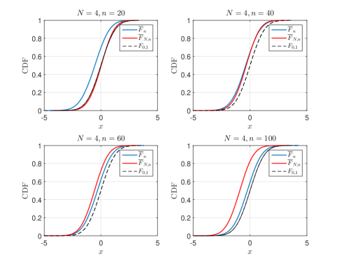
Figure 1: Empirical cumulative distribution functions (CDF) of $Q_{n}$ and $Q_{N,n}$ compared with the CDF of the standard Normal density for different values of $\left(N,n\right)$. $\rho=0.65$.

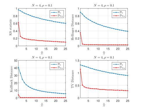
Figure 2: $\mathcal{D}_{n}$ and $\mathcal{D}_{N,n}$ as defined in (14) versus $\frac{n}{N}$. $\rho=0.1$.

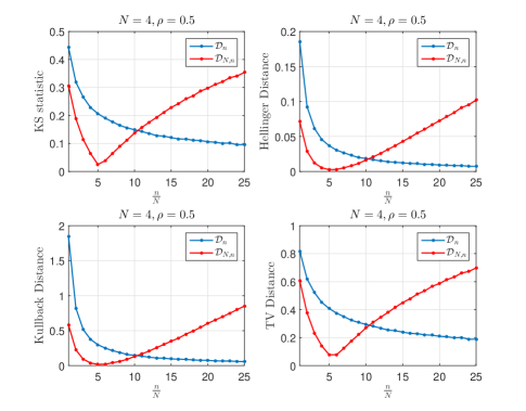
Figure 3: $\mathcal{D}_{n}$ and $\mathcal{D}_{N,n}$ as defined in (14) versus $\frac{n}{N}$. $\rho=0.5$.

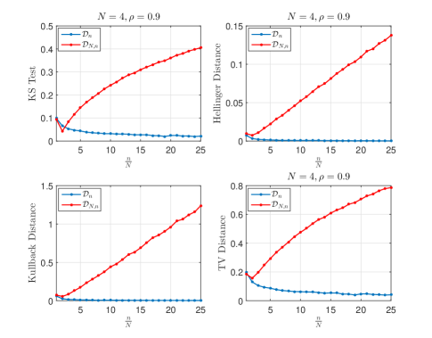
Figure 4: $\mathcal{D}_{n}$ and $\mathcal{D}_{N,n}$ as defined in (14) versus $\frac{n}{N}$. $\rho=0.9$.

To begin with, we report in Figure 1 the empirical CDFs of both regimes along with the standard normal CDF. As seen, the accuracy the $n$-large regime is lower than the $\left(N,n\right)$-large regime for small values of $n$. As the number of observations increases, the $\left(N,n\right)-$large regime becomes less accurate. This is to be compared with the $n-$large regime which provides a good fit for $n=60$ and $n=100$.

To reinforce the observations made in Figure 1, we display the distance between the empirical distributions $\overline{f}_{n}$ and $\overline{f}_{N,n}$ with the standard normal density for different values of $N$ and $n$. In order to investigate the impact of $\rho$ on the performance, we display the different instances of the distance for small ($\rho=0.1$ Figure 2), mid ($\rho=0.5$, Figure 3) and high ($\rho=0.9$, Figure 4) values of $\rho$.

• $\rho=0.1$: We observe in this case that the $(N,n)$-Large regime provides more accurate results. This might be related to the fact that the empirical average $\frac{1}{n}\sum_{i=1}^{n}\frac{\mathbf{x}_{i}\mathbf{x}_{i}^{*}}{\frac{1}{N}\mathbf{x}_{i}^{*}\widehat{\mathbf{C}}_{N}^{-1}(\rho)\mathbf{x}_{i}}$ is the dominant term in the expression of $\widehat{\bf C}_{N}(\rho)$. This averaging is approximated in the $n$-Large regime by $N\left(1-\rho\right)\mathbb{E}\left[\frac{\mathbf{x}\mathbf{x}^{*}}{\mathbf{x}^{*}\mathbf{\Sigma}_{0}^{-1}(\rho)\mathbf{x}}\right]$, which can be not well-estimated as $n$ is limited to $100$. On the other hand, the $(n,N)-$ large regime is more accurate since it leverages the double averaging over $n$ and $N$.

• $\rho=0.9$: In this case, $\rho$ is high, thus, the estimated SNR behaves as a deterministic quantity since $\widehat{\mathbf{C}}_{N}(\rho)\simeq\mathbf{I}_{N}$ which is the case for $\mathbf{\Sigma}_{0}(\rho)$ as well. This is clearly expected by the large$-n$ regime. However, the large$-(n,N)$ regime fails to predict in an accurate way the performances. One possible explanation can be related to the fact that as $\rho$ tends to $1$, quantity $\alpha(\rho)$ converges to infinity, causing the fluctuations to be not properly predicted.

• $\rho=0.5:$ In this case, the main observation is that the $\left(N,n\right)-$large regime has a better fit to the standard normal distribution for lower values of $n$, while for $\frac{n}{N}\geq 10$, the $n-$large regime starts to exhibit a better fit.

As a conclusion, for mid values of $\rho$, it is better to work under the $\left(N,n\right)-$large regime as long as the number of observations is low. As we get more observations, the $n-$large regime yields a better performance.

V Conclusion

In this paper, we have analyzed the asymptotic behaviour of the Capon’s MVDR beamformer when using the regularized Tyler estimator (RTE) for both the $n-$large and the $\left(N,n\right)-$large regimes. Based on recent results on the convergence of the RTE, we have analyzed the fluctuations of the SNR at the output of the MVDR. Using well known divergence metrics, we have examined the accuracy of both regimes and determined which regime is more accurate and thus more convenient to use.

Appendix A

Proof of Theorem 1

The proof hinges on recent results concerning the asymptotic behaviour of the RTE developed in [10] and the second order analysis of the SNR at the output of the MVDR derived in [12]. As we shall see next, these results lead together to the sought-for CLT.

V-1 First ingredient: Approximation of the RTE estimate $\widehat{\mathbf{C}}_{N}(\rho)$

Studying the RTE in the large$-n,N$ regime is not an easy task, as the RTE does not follow a standard random matrix model. To overcome these issues, the work in [10] shows that as far as quadratic forms are concerned the asymptotic behaviour of the $\widehat{\mathbf{C}}_{N}(\rho)$ is the same as another random object which, contrary to $\widehat{\mathbf{C}}_{N}(\rho)$ can be studied using standard RMT tools. More formally, we have the following convergence results,

$$N^{1-\epsilon}|\mathbf{u}^{*}\widehat{\mathbf{C}}^{k}_{N}(\rho)\mathbf{v}-\mathbf{u}^{*}\widehat{\mathbf{S}}^{k}_{N}(\rho)\mathbf{v}|\xrightarrow[]{a.s.}0,$$ (15)

where $\mathbf{u}$ and $\mathbf{v}$ are unit norm vectors in $\mathbb{C}^{N}$ and $\widehat{\bf S}_{N}(\rho)$ is given by

$$\widehat{\mathbf{S}}_{N}(\rho)=\frac{\rho}{\alpha\left(\rho\right)}\frac{1}{n}\sum_{i=1}^{n}\mathbf{z}_{i}\mathbf{z}_{i}^{*}+\rho\mathbf{I}_{N},\mathbf{z}_{i}=\mathbf{\Sigma}_{N}^{\frac{1}{2}}\mathbf{w}_{i},\>i=1,\cdots,n.$$

As will be shown next, this convergence implies that the SNR has the same fluctuations if $\widehat{\bf C}_{N}$ is replaced by $\widehat{\mathbf{S}}_{N}(\rho)$.

As the SNR is scale invariant, the fluctuations would be the same when $\widehat{\bf C}_{N}$ is replaced by $\widetilde{\bf S}_{N}(\rho)$ given by:

$$\widetilde{\bf S}_{N}(\rho)=\frac{1}{n}\sum_{i=1}^{n}\mathbf{z}_{i}\mathbf{z}_{i}^{*}+\alpha\left(\rho\right)\mathbf{I}_{N}.$$ (16)

Interestingly, the approximation matrix in (16) follows the same structure of a sample correlation matrix with a diagonal loading factor $\alpha\left(\rho\right)$ that was considered in [11]. The fluctuations of the SNR will be thus obtained by simply leveraging the results of [11].

V-2 Second-order Analysis of the SNR of Diagonally Loaded MVDR Filters

As discussed above, to prove Theorem 1, it suffices to show that the SNR has the same fluctuations when the RTE is replaced by $\widehat{\bf S}_{N}(\rho)$. As per the Slutsky Lemma, this amounts to showing that:

$$\sqrt{n}\left(\frac{\left(\mathbf{s^{*}_{0}}\widehat{\mathbf{C}}_{N}^{-1}(\rho)\mathbf{s_{0}}\right)^{2}}{\mathbf{s^{*}_{0}}\widehat{\mathbf{C}}_{N}^{-1}(\rho)\mathbf{\Sigma}_{N}\widehat{\mathbf{C}}_{N}^{-1}(\rho)\mathbf{s_{0}}}-\frac{\left(\mathbf{s^{*}_{0}}\widehat{\mathbf{S}}_{N}^{-1}(\rho)\mathbf{s_{0}}\right)^{2}}{\mathbf{s^{*}_{0}}\widehat{\mathbf{S}}_{N}^{-1}(\rho)\mathbf{\Sigma}_{N}\widehat{\mathbf{S}}_{N}^{-1}(\rho)\mathbf{s_{0}}}\right)$$

$$\xrightarrow[\frac{N}{n}\to c]{a.s.}0.$$

To this end, we first decompose the above term as:

$$\sqrt{n}\left(\frac{\left(\mathbf{s^{*}_{0}}\widehat{\mathbf{C}}_{N}^{-1}(\rho)\mathbf{s_{0}}\right)^{2}}{\mathbf{s^{*}_{0}}\widehat{\mathbf{C}}_{N}^{-1}(\rho)\mathbf{\Sigma}_{N}\widehat{\mathbf{C}}_{N}^{-1}(\rho)\mathbf{s_{0}}}-\frac{\left(\mathbf{s^{*}_{0}}\widehat{\mathbf{S}}_{N}^{-1}(\rho)\mathbf{s_{0}}\right)^{2}}{\mathbf{s^{*}_{0}}\widehat{\mathbf{S}}_{N}^{-1}(\rho)\mathbf{\Sigma}_{N}\widehat{\mathbf{S}}_{N}^{-1}(\rho)\mathbf{s_{0}}}\right)$$

$$=\sqrt{n}\left(\frac{\left(\mathbf{s^{*}_{0}}\widehat{\mathbf{C}}_{N}^{-1}(\rho)\mathbf{s_{0}}\right)^{2}}{\mathbf{s^{*}_{0}}\widehat{\mathbf{C}}_{N}^{-1}(\rho)\mathbf{\Sigma}_{N}\widehat{\mathbf{C}}_{N}^{-1}(\rho)\mathbf{s_{0}}}-\frac{\left(\mathbf{s^{*}_{0}}\widehat{\mathbf{S}}_{N}^{-1}(\rho)\mathbf{s_{0}}\right)^{2}}{\mathbf{s^{*}_{0}}\widehat{\mathbf{C}}_{N}^{-1}(\rho)\mathbf{\Sigma}_{N}\widehat{\mathbf{C}}_{N}^{-1}(\rho)\mathbf{s_{0}}}\right)$$

$$+\sqrt{n}\left(\frac{\left(\mathbf{s^{*}_{0}}\widehat{\mathbf{S}}_{N}^{-1}(\rho)\mathbf{s_{0}}\right)^{2}}{\mathbf{s^{*}_{0}}\widehat{\mathbf{C}}_{N}^{-1}(\rho)\mathbf{\Sigma}_{N}\widehat{\mathbf{C}}_{N}^{-1}(\rho)\mathbf{s_{0}}}-\frac{\left(\mathbf{s^{*}_{0}}\widehat{\mathbf{S}}_{N}^{-1}(\rho)\mathbf{s_{0}}\right)^{2}}{\mathbf{s^{*}_{0}}\widehat{\mathbf{S}}_{N}^{-1}(\rho)\mathbf{\Sigma}_{N}\widehat{\mathbf{S}}_{N}^{-1}(\rho)\mathbf{s_{0}}}\right)$$

$$\triangleq\xi_{1}+\xi_{2}.$$

The term $\xi_{1}$ can be rewritten as

$$\begin{split}\xi_{1}&=\frac{\sqrt{n}\left(\mathbf{s^{*}_{0}}\widehat{\mathbf{C}}_{N}^{-1}(\rho)\mathbf{s_{0}}-\mathbf{s^{*}_{0}}\widehat{\mathbf{S}}_{N}^{-1}(\rho)\mathbf{s_{0}}\right)}{\mathbf{s^{*}_{0}}\widehat{\mathbf{C}}_{N}^{-1}(\rho)\mathbf{\Sigma}_{N}\widehat{\mathbf{C}}_{N}^{-1}(\rho)\mathbf{s_{0}}}.\\ &\times\left(\mathbf{s^{*}_{0}}\widehat{\mathbf{C}}_{N}^{-1}(\rho)\mathbf{s_{0}}+\mathbf{s^{*}_{0}}\widehat{\mathbf{S}}_{N}^{-1}(\rho)\mathbf{s_{0}}\right)\end{split}$$ (17)

Then, by the results of (22), we have the following convergence

$$\sqrt{n}\left(\mathbf{s^{*}_{0}}\widehat{\mathbf{C}}_{N}^{-1}(\rho)\mathbf{s_{0}}-\mathbf{s^{*}_{0}}\widehat{\mathbf{S}}_{N}^{-1}(\rho)\mathbf{s_{0}}\right)\xrightarrow[\frac{N}{n}\to c]{a.s.}0$$

Moreover, since,

$$\left\|\widehat{\mathbf{C}}_{N}^{-1}(\rho)-\widehat{\mathbf{S}}_{N}^{-1}(\rho)\right\|\xrightarrow[]{a.s.}0.$$

then, any well-behaved functional of $\widehat{\mathbf{C}}_{N}^{-1}(\rho)$ converges $a.s.$ to the same functional of $\widehat{\mathbf{S}}_{N}^{-1}(\rho)$. In particular, we do have:

$$\mathbf{s^{*}_{0}}\widehat{\mathbf{C}}_{N}^{-1}(\rho)\mathbf{s_{0}}-\mathbf{s^{*}_{0}}\widehat{\mathbf{S}}_{N}^{-1}(\rho)\mathbf{s_{0}}\xrightarrow[\frac{N}{n}\to c]{a.s.}0.$$

and

$$\mathbf{s^{*}_{0}}\widehat{\mathbf{C}}_{N}^{-1}(\rho)\mathbf{\Sigma}_{N}\widehat{\mathbf{C}}_{N}^{-1}(\rho)\mathbf{s_{0}}-\mathbf{s^{*}_{0}}\widehat{\mathbf{S}}_{N}^{-1}(\rho)\mathbf{\Sigma}_{N}\widehat{\mathbf{S}}_{N}^{-1}(\rho)\mathbf{s_{0}}\xrightarrow[]{a.s.}0.$$

All this leads to

$$\xi_{1}\xrightarrow[\frac{N}{n}\to c]{P}0.$$

We now handle the term $\xi_{2}$. By a similar reasoning, $\xi_{2}$ can be rewritten as follows

$$\xi_{2} =$$

$$\frac{\left(\mathbf{s^{*}_{0}}\widehat{\mathbf{S}}_{N}^{-1}(\rho)\mathbf{s_{0}}\right)^{2}}{\left(\mathbf{s^{*}_{0}}\widehat{\mathbf{C}}_{N}^{-1}(\rho)\mathbf{\Sigma}_{N}\widehat{\mathbf{C}}_{N}^{-1}(\rho)\mathbf{s_{0}}\right)\left(\mathbf{s^{*}_{0}}\widehat{\mathbf{S}}_{N}^{-1}(\rho)\mathbf{\Sigma}_{N}\widehat{\mathbf{S}}_{N}^{-1}(\rho)\mathbf{s_{0}}\right)}$$

$$\times\sqrt{n}\left(\mathbf{s^{*}_{0}}\widehat{\mathbf{S}}_{N}^{-1}(\rho)\mathbf{\Sigma}_{N}\widehat{\mathbf{S}}_{N}^{-1}(\rho)\mathbf{s_{0}}-\mathbf{s^{*}_{0}}\widehat{\mathbf{C}}_{N}^{-1}(\rho)\mathbf{\Sigma}_{N}\widehat{\mathbf{C}}_{N}^{-1}(\rho)\mathbf{s_{0}}\right).$$

We now refer to the special structure of $\mathbf{\Sigma}_{N}$ and rewrite $\xi_{2}$ as follows

$$\xi_{2} =\frac{\left(\mathbf{s^{*}_{0}}\widehat{\mathbf{S}}_{N}^{-1}(\rho)\mathbf{s_{0}}\right)^{2}}{\left(\mathbf{s^{*}_{0}}\widehat{\mathbf{C}}_{N}^{-1}(\rho)\mathbf{\Sigma}_{N}\widehat{\mathbf{C}}_{N}^{-1}(\rho)\mathbf{s_{0}}\right)\left(\mathbf{s^{*}_{0}}\widehat{\mathbf{S}}_{N}^{-1}(\rho)\mathbf{\Sigma}_{N}\widehat{\mathbf{S}}_{N}^{-1}(\rho)\mathbf{s_{0}}\right)}$$

$$\times\sqrt{n}\Biggl{[}\sigma_{0}^{2}\left(\mathbf{s^{*}_{0}}\widehat{\mathbf{S}}_{N}^{-2}(\rho)\mathbf{s_{0}}-\mathbf{s^{*}_{0}}\widehat{\mathbf{C}}_{N}^{-2}(\rho)\mathbf{s_{0}}\right)$$

$$+\sum_{i=1}^{q}\sigma_{i}^{2}\left(|\mathbf{s^{*}_{0}}\widehat{\mathbf{S}}_{N}^{-1}(\rho)\mathbf{a}\left(\theta_{i}\right)|^{2}-|\mathbf{s^{*}_{0}}\widehat{\mathbf{C}}_{N}^{-1}(\rho)\mathbf{a}\left(\theta_{i}\right)|^{2}\right)\Biggr{]}.$$

Noticing that

$$|\mathbf{s^{*}_{0}}\widehat{\mathbf{S}}_{N}^{-1}(\rho)\mathbf{a}\left(\theta_{i}\right)|^{2}-|\mathbf{s^{*}_{0}}\widehat{\mathbf{C}}_{N}^{-1}(\rho)\mathbf{a}\left(\theta_{i}\right)|^{2}$$

$$=\left(|\mathbf{s^{*}_{0}}\widehat{\mathbf{S}}_{N}^{-1}(\rho)\mathbf{a}\left(\theta_{i}\right)|-|\mathbf{s^{*}_{0}}\widehat{\mathbf{C}}_{N}^{-1}(\rho)\mathbf{a}\left(\theta_{i}\right)|\right)$$

$$\times\left(|\mathbf{s^{*}_{0}}\widehat{\mathbf{S}}_{N}^{-1}(\rho)\mathbf{a}\left(\theta_{i}\right)|+|\mathbf{s^{*}_{0}}\widehat{\mathbf{C}}_{N}^{-1}(\rho)\mathbf{a}\left(\theta_{i}\right)|\right).$$

and resorting to the same arguments used in the control of $\xi_{1}$, it follows that

$$\xi_{2}\xrightarrow[\frac{N}{n}\to c]{a.s.}0.$$

This concludes the proof of Theorem 1.

Appendix B

Proof of Theorem 2

For ease of presentation, we omit the argument $\rho$ in the SNR expressions. According to [8], the asymptotic limit of $\widehat{\textnormal{SNR}}$ would be

$$\textnormal{SNR}_{0}=\frac{\left(\mathbf{s^{*}_{0}}\mathbf{\Sigma}_{0}^{-1}(\rho)\mathbf{s_{0}}\right)^{2}}{\mathbf{s^{*}_{0}}\mathbf{\Sigma}_{0}^{-1}(\rho)\mathbf{\Sigma}_{N}\mathbf{\Sigma}_{0}^{-1}(\rho)\mathbf{s_{0}}}.$$

The objective here is to study the fluctuations of the SNR around $\textnormal{SNR}_{0}$. To this end, we decompose $\sqrt{n}\left(\widehat{\textnormal{SNR}}-\textnormal{SNR}_{0}\right)$ by subtracting and adding $\sqrt{n}\frac{\left(\mathbf{s^{*}_{0}}\mathbf{\Sigma}_{0}^{-1}(\rho)\mathbf{s_{0}}\right)^{2}}{\mathbf{s^{*}_{0}}\widehat{\mathbf{C}}^{-1}_{N}(\rho)\mathbf{\Sigma}_{N}\widehat{\mathbf{C}}^{-1}_{N}(\rho)\mathbf{s_{0}}}$ resulting in expression (18) given on the top of the next page.

$$\begin{split}&\sqrt{n}\left(\widehat{\textnormal{SNR}}-\textnormal{SNR}_{0}\right)=\\ &\underbrace{\frac{\sqrt{n}}{\mathbf{s^{*}_{0}}\widehat{\mathbf{C}}^{-1}_{N}(\rho)\mathbf{\Sigma}_{N}\widehat{\mathbf{C}}^{-1}_{N}(\rho)\mathbf{s_{0}}}\left(\mathbf{s^{*}_{0}}\widehat{\mathbf{C}}^{-1}_{N}(\rho)\mathbf{s_{0}}-\mathbf{s^{*}_{0}}\mathbf{\Sigma}_{0}^{-1}(\rho)\mathbf{s_{0}}\right)\left(\mathbf{s^{*}_{0}}\widehat{\mathbf{C}}^{-1}_{N}(\rho)\mathbf{s_{0}}+\mathbf{s^{*}_{0}}\mathbf{\Sigma}_{0}^{-1}(\rho)\mathbf{s_{0}}\right)}_{Q_{1}}\\ &+\underbrace{\frac{\sqrt{n}\left(\mathbf{s^{*}_{0}}\mathbf{\Sigma}_{0}^{-1}(\rho)\mathbf{s_{0}}\right)^{2}}{\left(\mathbf{s^{*}_{0}}\widehat{\mathbf{C}}^{-1}_{N}(\rho)\mathbf{\Sigma}_{N}\widehat{\mathbf{C}}^{-1}_{N}(\rho)\mathbf{s_{0}}\right)\left(\mathbf{s^{*}_{0}}\mathbf{\Sigma}_{0}^{-1}(\rho)\mathbf{\Sigma}_{N}\mathbf{\Sigma}_{0}^{-1}(\rho)\mathbf{s_{0}}\right)}\left(\mathbf{s^{*}_{0}}\mathbf{\Sigma}_{0}^{-1}(\rho)\mathbf{\Sigma}_{N}\mathbf{\Sigma}_{0}^{-1}(\rho)\mathbf{s_{0}}-\mathbf{s^{*}_{0}}\widehat{\mathbf{C}}^{-1}_{N}(\rho)\mathbf{\Sigma}_{N}\widehat{\mathbf{C}}^{-1}_{N}(\rho)\mathbf{s_{0}}\right)}_{Q_{2}}\end{split}.$$ (18)

We will now treat subsequently the terms $Q_{1}$ and $Q_{2}$ defined in (18). First, note that using the resolvent identity:

$$\widehat{\mathbf{C}}^{-1}_{N}(\rho)-\mathbf{\Sigma}_{0}^{-1}(\rho)=\widehat{\mathbf{C}}^{-1}_{N}(\rho)\left(\mathbf{\Sigma}_{0}(\rho)-\widehat{\mathbf{C}}_{N}(\rho)\right)\mathbf{\Sigma}_{0}^{-1}(\rho).$$ (19)

along with the relation:

$$\mathbf{x^{*}}\mathbf{A}\mathbf{y} =\textnormal{tr}\left(\mathbf{x^{*}}\mathbf{A}\mathbf{y}\right)$$

$$=\textnormal{vec}^{*}(\mathbf{x})\textnormal{vec}\left(\mathbf{Ay}\right)$$

$$=\mathbf{x}^{*}\left(\mathbf{y^{t}}\otimes\mathbf{I}_{N}\right)\textnormal{vec}(\mathbf{A}).$$

for ${\bf x}\in\mathbb{C}^{N\times 1},{\bf y}\in\mathbb{C}^{N\times 1}$ and ${\bf A}\in\mathbb{C}^{N\times N}$, yields

$$\sqrt{n}\>\mathbf{s^{*}_{0}}\left(\widehat{\mathbf{C}}^{-1}_{N}(\rho)-\mathbf{\Sigma}_{0}^{-1}(\rho)\right)\mathbf{s_{0}}$$

$$=\sqrt{n}\>\mathbf{s^{*}_{0}}\widehat{\mathbf{C}}^{-1}_{N}(\rho)\left(\mathbf{\Sigma}_{0}(\rho)-\widehat{\mathbf{C}}_{N}(\rho)\right)\mathbf{\Sigma}_{0}^{-1}(\rho)\mathbf{s_{0}}$$

$$=\sqrt{n}\>\mathbf{s^{*}_{0}}\widehat{\mathbf{C}}^{-1}_{N}(\rho)\left[\left(\mathbf{s_{0}^{t}}\mathbf{\Sigma}_{0}^{-1}(\rho)\right)\otimes\mathbf{I}_{N}\right]$$

$$\times\textnormal{vec}\left(\mathbf{\Sigma}_{0}(\rho)-\widehat{\mathbf{C}}_{N}(\rho)\right).$$

Using the result of Lemma 1, we have

$$\sqrt{n}\>\textnormal{vec}\left(\widehat{\mathbf{C}}_{N}(\rho)-\mathbf{\Sigma}_{0}(\rho)\right)\xrightarrow[n\to+\infty]{d}\mathbf{x}\sim\mathcal{GCN}\left(0,\mathbf{M}_{1},\mathbf{M}_{2}\right),$$

where $\mathcal{GCN}\left(\mathbf{0},\mathbf{M}_{1},\mathbf{M}_{2}\right)$ denotes the Generalized Complex Normal distribution with zero-mean, covariance matrix $\mathbf{M}_{1}$ and pseudo-covariance matrix $\mathbf{M}_{2}$. Finally, using the following convergence relations

$$\mathbf{s^{*}_{0}}\widehat{\mathbf{C}}^{-1}_{N}(\rho)\left[\left(\mathbf{s_{0}^{t}}\mathbf{\Sigma}_{0}^{-1}(\rho)\right)\otimes\mathbf{I}_{N}\right]$$

$$\xrightarrow[n\to+\infty]{a.s}\mathbf{s^{*}_{0}}\mathbf{\Sigma}_{0}^{-1}(\rho)\left[\left(\mathbf{s_{0}^{t}}\mathbf{\Sigma}_{0}^{-1}(\rho)\right)\otimes\mathbf{I}_{N}\right].$$

$$\mathbf{s^{*}_{0}}\widehat{\mathbf{C}}^{-1}_{N}(\rho)\mathbf{s_{0}}+\mathbf{s^{*}_{0}}\mathbf{\Sigma}_{0}^{-1}(\rho)\mathbf{s_{0}}\xrightarrow[n\to+\infty]{a.s}2\>\mathbf{s^{*}_{0}}\mathbf{\Sigma}_{0}^{-1}(\rho)\mathbf{s_{0}}.$$

$$\frac{1}{\mathbf{s^{*}_{0}}\widehat{\mathbf{C}}^{-1}_{N}(\rho)\mathbf{\Sigma}_{N}\widehat{\mathbf{C}}^{-1}_{N}(\rho)\mathbf{s_{0}}}\xrightarrow[n\to+\infty]{a.s}\frac{1}{\mathbf{s^{*}_{0}}\mathbf{\Sigma}_{0}^{-1}(\rho)\mathbf{\Sigma}_{N}\mathbf{\Sigma}_{0}^{-1}(\rho)\mathbf{s_{0}}}.$$

it follows from the Slutsky’s theorem [17] that:

$$\begin{split}Q_{1}\xrightarrow[n\to+\infty]{d}&\frac{-2\>\mathbf{s^{*}_{0}}\mathbf{\Sigma}_{0}^{-1}(\rho)\mathbf{s_{0}}}{\mathbf{s^{*}_{0}}\mathbf{\Sigma}_{0}^{-1}(\rho)\mathbf{\Sigma}_{N}\mathbf{\Sigma}_{0}^{-1}(\rho)\mathbf{s_{0}}}\mathbf{s^{*}_{0}}\mathbf{\Sigma}_{0}^{-1}(\rho)\\ &\times\left[\left(\mathbf{s_{0}^{t}}\mathbf{\Sigma}_{0}^{-1}(\rho)\right)\otimes\mathbf{I}_{N}\right]\mathbf{x}\end{split}.$$ (20)

We now handle $Q_{2}$. To this end, we treat the term $\sqrt{n}\>\left(\mathbf{s^{*}_{0}}\mathbf{\Sigma}_{0}^{-1}(\rho)\mathbf{\Sigma}_{N}\mathbf{\Sigma}_{0}^{-1}(\rho)\mathbf{s_{0}}-\mathbf{s^{*}_{0}}\widehat{\mathbf{C}}^{-1}_{N}(\rho)\mathbf{\Sigma}_{N}\widehat{\mathbf{C}}^{-1}_{N}(\rho)\mathbf{s_{0}}\right)$ as follows

$$\sqrt{n}\>\left(\mathbf{s^{*}_{0}}\mathbf{\Sigma}_{0}^{-1}(\rho)\mathbf{\Sigma}_{N}\mathbf{\Sigma}_{0}^{-1}(\rho)\mathbf{s_{0}}-\mathbf{s^{*}_{0}}\widehat{\mathbf{C}}^{-1}_{N}(\rho)\mathbf{\Sigma}_{N}\widehat{\mathbf{C}}^{-1}_{N}(\rho)\mathbf{s_{0}}\right)$$

$$=\sqrt{n}\>\Biggl{(}\mathbf{s^{*}_{0}}\mathbf{\Sigma}_{0}^{-1}(\rho)\mathbf{\Sigma}_{N}\mathbf{\Sigma}_{0}^{-1}(\rho)\mathbf{s_{0}}-\mathbf{s^{*}_{0}}\mathbf{\Sigma}_{0}^{-1}(\rho)\mathbf{\Sigma}_{N}\widehat{\mathbf{C}}^{-1}_{N}(\rho)\mathbf{s_{0}}$$

$$+\mathbf{s^{*}_{0}}\mathbf{\Sigma}_{0}^{-1}(\rho)\mathbf{\Sigma}_{N}\widehat{\mathbf{C}}^{-1}_{N}(\rho)\mathbf{s_{0}}-\mathbf{s^{*}_{0}}\widehat{\mathbf{C}}^{-1}_{N}(\rho)\mathbf{\Sigma}_{N}\widehat{\mathbf{C}}^{-1}_{N}(\rho)\mathbf{s_{0}}\Biggr{)}$$

$$=\sqrt{n}\>\mathbf{s^{*}_{0}}\mathbf{\Sigma}_{0}^{-1}(\rho)\mathbf{\Sigma}_{N}\left(\mathbf{\Sigma}_{0}^{-1}(\rho)-\widehat{\mathbf{C}}^{-1}_{N}(\rho)\right)\mathbf{s_{0}}$$

$$+\sqrt{n}\>\mathbf{s^{*}_{0}}\left(\mathbf{\Sigma}_{0}^{-1}(\rho)-\widehat{\mathbf{C}}^{-1}_{N}(\rho)\right)\mathbf{\Sigma}_{N}\widehat{\mathbf{C}}^{-1}_{N}(\rho)\mathbf{s_{0}}.$$

Similarly, using the resolvent identity, we can write

$$\sqrt{n}\>\left(\mathbf{s^{*}_{0}}\mathbf{\Sigma}_{0}^{-1}(\rho)\mathbf{\Sigma}_{N}\mathbf{\Sigma}_{0}^{-1}(\rho)\mathbf{s_{0}}-\mathbf{s^{*}_{0}}\widehat{\mathbf{C}}^{-1}_{N}(\rho)\mathbf{\Sigma}_{N}\widehat{\mathbf{C}}^{-1}_{N}(\rho)\mathbf{s_{0}}\right)$$

$$=\sqrt{n}\>\mathbf{s^{*}_{0}}\mathbf{\Sigma}_{0}^{-1}(\rho)\mathbf{\Sigma}_{N}\mathbf{\Sigma}_{0}^{-1}(\rho)\left(\widehat{\mathbf{C}}_{N}(\rho)-\mathbf{\Sigma}_{0}(\rho)\right)\widehat{\mathbf{C}}^{-1}_{N}(\rho)\mathbf{s_{0}}$$

$$+\sqrt{n}\>\mathbf{s^{*}_{0}}\mathbf{\Sigma}_{0}^{-1}(\rho)\left(\widehat{\mathbf{C}}_{N}(\rho)-\mathbf{\Sigma}_{0}(\rho)\right)\widehat{\mathbf{C}}^{-1}_{N}(\rho)\mathbf{\Sigma}_{N}\widehat{\mathbf{C}}^{-1}_{N}(\rho)\mathbf{s_{0}}$$

$$=\sqrt{n}\>\mathbf{s^{*}_{0}}\mathbf{\Sigma}_{0}^{-1}(\rho)\mathbf{\Sigma}_{N}\mathbf{\Sigma}_{0}^{-1}(\rho)\left[\left(\mathbf{s_{0}^{t}}\widehat{\mathbf{C}}^{-1}_{N}(\rho)\right)\otimes\mathbf{I}_{N}\right]$$

$$\times\textnormal{vec}\left(\widehat{\mathbf{C}}_{N}(\rho)-\mathbf{\Sigma}_{0}(\rho)\right)+\sqrt{n}\>\mathbf{s^{*}_{0}}\mathbf{\Sigma}_{0}^{-1}(\rho)$$

$$\times\left[\left(\widehat{\mathbf{C}}^{-1}_{N}(\rho)\mathbf{\Sigma}_{N}\widehat{\mathbf{C}}^{-1}_{N}(\rho)\mathbf{s_{0}}\right)^{t}\otimes\mathbf{I}_{N}\right]\textnormal{vec}\left(\widehat{\mathbf{C}}_{N}(\rho)-\mathbf{\Sigma}_{0}(\rho)\right).$$

Also note that

$$\frac{\left(\mathbf{s^{*}_{0}}\mathbf{\Sigma}_{0}^{-1}(\rho)\mathbf{s_{0}}\right)^{2}}{\left(\mathbf{s^{*}_{0}}\widehat{\mathbf{C}}^{-1}_{N}(\rho)\mathbf{\Sigma}_{N}\widehat{\mathbf{C}}^{-1}_{N}(\rho)\mathbf{s_{0}}\right)\left(\mathbf{s^{*}_{0}}\mathbf{\Sigma}_{0}^{-1}(\rho)\mathbf{\Sigma}_{N}\mathbf{\Sigma}_{0}^{-1}(\rho)\mathbf{s_{0}}\right)}$$

$$\xrightarrow[n\to+\infty]{a.s}\frac{\left(\mathbf{s^{*}_{0}}\mathbf{\Sigma}_{0}^{-1}(\rho)\mathbf{s_{0}}\right)^{2}}{\left(\mathbf{s^{*}_{0}}\mathbf{\Sigma}_{0}^{-1}(\rho)\mathbf{\Sigma}_{N}\mathbf{\Sigma}_{0}^{-1}(\rho)\mathbf{s_{0}}\right)^{2}}$$

Thus, by means of Slutsky’s theorem, it follows that

$$Q_{2}\xrightarrow[n\to+\infty]{d} \frac{\left(\mathbf{s^{*}_{0}}\mathbf{\Sigma}_{0}^{-1}(\rho)\mathbf{s_{0}}\right)^{2}}{\left(\mathbf{s^{*}_{0}}\mathbf{\Sigma}_{0}^{-1}(\rho)\mathbf{\Sigma}_{N}\mathbf{\Sigma}_{0}^{-1}(\rho)\mathbf{s_{0}}\right)^{2}}\Biggl{[}\mathbf{s^{*}_{0}}\mathbf{\Sigma}_{0}^{-1}(\rho)\mathbf{\Sigma}_{N}\mathbf{\Sigma}_{0}^{-1}(\rho)$$

$$\times\left[\left(\mathbf{s_{0}^{t}}\mathbf{\Sigma}_{0}^{-1}(\rho)\right)\otimes\mathbf{I}_{N}\right]+\mathbf{s^{*}_{0}}\mathbf{\Sigma}_{0}^{-1}(\rho)$$

$$\times\left[\left(\mathbf{\Sigma}_{0}^{-1}(\rho)\mathbf{\Sigma}_{N}\mathbf{\Sigma}_{0}^{-1}(\rho)\mathbf{s_{0}}\right)^{t}\otimes\mathbf{I}_{N}\right]\Biggr{]}\mathbf{x}.$$

Gathering the convergence results of $Q_{1}$ and $Q_{2}$, we thus obtain:

$$\sqrt{n}\left(\widehat{\textnormal{SNR}}-\textnormal{SNR}_{0}\right)\xrightarrow[n\to+\infty]{d}\mathbf{c^{*}}\mathbf{x}.$$

Noticing that

$$\begin{split}\mathbf{c^{*}}\mathbf{x}&=\Re(\mathbf{c})^{t}\Re(\mathbf{x})+\Im(\mathbf{c})^{t}\Im(\mathbf{c})\\ &=\widetilde{\mathbf{c}}^{t}\mathbf{v},\end{split}$$ (21)

where $\mathbf{v}=\left[\Re(\mathbf{x})^{t}\Im(\mathbf{x})^{t}\right]^{t}$, it suffices thus to derive the distribution of $\mathbf{v}$. This follows from the following Lemma:

Lemma 2.

Let $\mathbf{x}=\left(x_{1},x_{2},\cdots,x_{k}\right)^{t}$ be a zero-mean complex jointly-Gaussian random vector with covariance $\mathbf{M}_{1}$ and pseudo-covariance $\mathbf{M}_{2}$ and let $\mathbf{v}=\left[\Re(\mathbf{x})^{t}\Im(\mathbf{x})^{t}\right]^{t}$. Then, following the results of [18],

$$\mathbf{v}\sim\mathcal{N}\left(\mathbf{0},\Xi\right)$$ (22)

Using Lemma 22, we conculde that $\mathbf{c^{*}}\mathbf{x}$ is normally distributed with zero mean and variance $\sigma_{n}^{2}=\widetilde{\mathbf{c}}^{t}\Xi\widetilde{\mathbf{c}}$. This conculdes the proof of the theorem.

References

- [1] H. V. Trees, Optimum Array Processing. New York: Wiley, 2002.
- [2] P. Stoica and R. Moses, Spectral Analysis of Signals. Englewood Cliffs, NJ: Prentice-Hall, 2005, vol. 1.
- [3] K. D. Ward, “Compound representation of high resolution sea clutter,” Electronics Letters, vol. 17, no. 16, p. 561–563, August 1981.
- [4] S. Watts, “Radar detection prediction in sea clutter using the compound k-distribution model,” Communications, Radar and Signal Processing, IEE Proceedings F, vol. 132, no. 7, pp. 613–620, December 1985.
- [5] T. Nohara and S. Haykin, “Canadian east coast radar trials and the k-distribution,” Radar and Signal Processing, IEE Proceedings F, vol. 138, no. 2, pp. 80–88, April 1991.
- [6] P. J. Huber, Robust Statistics. Wiley Series in Probability and Statistics John Wiley& Sons, 1981.
- [7] R. A. Maronna, “Robust M-estimators of multivariate location and scatter,” The Annals of Statistics, no. 4, pp. 51–67, 1976.
- [8] A. Kammoun, R. Couillet, F. Pascal, and M.-S. Alouini, “Convergence and fluctuations of regularized tyler estimators,” Submitted to IEEE Transactions on Signal Processing, 2015. [Online]. Available: http://arxiv.org/abs/1504.01252
- [9] R. Couillet and M. McKay, “Large dimensional analysis and optimization of robust shrinkage covariance matrix estimators,” Journal of Multivariate Analysis, vol. 131, pp. 99–120, 2014.
- [10] R. Couillet, A. Kammoun, and F. Pascal, “Second Order Statistics of Robust Estimators of Scatter. Application to GLRT Detection for Elliptical Signals,” Journal of Multivariate Analysis, vol. 143, pp. 249–274, Jan 2016.
- [11] X. Mestre and M. Lagunas, “Finite Sample Size Effect on Minimum Variance Beamformers: Optimum Diagonal Loading Factor for Large Arrays,” IEEE Transactions on Signal Processing, vol. 54, no. 1, pp. 69–82, Jan 2006.
- [12] F. Rubio, X. Mestre, and W. Hachem, “A CLT on the SNR of Diagonally Loaded MVDR Filters,” IEEE Transactions of Signal Processing, vol. 60, no. 8, Aug. 2012.
- [13] D. Li, Q. Yin, P. Mu, and W. Guo, “Robust MVDR beamforming using the DOA matrix decomposition,” in Access Spaces (ISAS), 2011 1st International Symposium on, June 2011, pp. 105–110.
- [14] F. Pascal, Y. Chitour, and Y. Quek, “Generalized Robust Shrinkage Esitmator and Its Application to STAP Detection Problem ,” IEEE Transactions on Signal Processing, vol. 62, no. 21, pp. 5640–5651, 2014.
- [15] F. Rubio and X. Mestre, “Design of reduced-rank mvdr beamformers under finite sample-support,” in Fourth IEEE Workshop on Sensor Array and Multichannel Processing,, July 2006, pp. 31–35.
- [16] R. Qian, M. Sellathurai, and D. Wilcox, “A Study On MVDR Beamforming Applied To An ESPAR Antenna,” Signal Processing Letters, IEEE, vol. 22, no. 1, pp. 67–70, Jan 2015.
- [17] D. D. Boos and L. A. Stefanski, Essential Statistical Inference. Springer, 2013.
- [18] R. G. Gallager, “Circularly-Symmetric Gaussian Random Vectors,” 2008. [Online]. Available: http://www.rle.mit.edu/rgallager/documents/CircSymGauss.pdf