Nonlinear Preconditioning: How to use a Nonlinear Schwarz Method to Precondition Newton’s Method

Abstract

For linear problems, domain decomposition methods can be used directly as iterative solvers, but also as preconditioners for Krylov methods. In practice, Krylov acceleration is almost always used, since the Krylov method finds a much better residual polynomial than the stationary iteration, and thus converges much faster. We show in this paper that also for non-linear problems, domain decomposition methods can either be used directly as iterative solvers, or one can use them as preconditioners for Newton’s method. For the concrete case of the parallel Schwarz method, we show that we obtain a preconditioner we call RASPEN (Restricted Additive Schwarz Preconditioned Exact Newton) which is similar to ASPIN (Additive Schwarz Preconditioned Inexact Newton), but with all components directly defined by the iterative method. This has the advantage that RASPEN already converges when used as an iterative solver, in contrast to ASPIN, and we thus get a substantially better preconditioner for Newton’s method. The iterative construction also allows us to naturally define a coarse correction using the multigrid full approximation scheme, which leads to a convergent two level non-linear iterative domain decomposition method and a two level RASPEN non-linear preconditioner. We illustrate our findings with numerical results on the Forchheimer equation and a non-linear diffusion problem.

1 Introduction

Non-linear partial differential equations are usually solved after discretization by Newton’s method or variants thereof. While Newton’s method converges well from an initial guess close to the solution, its convergence behaviour can be erratic and the method can lose all its effectiveness if the initial guess is too far from the solution. Instead of using Newton, one can use a domain decomposition iteration, applied directly to the non-linear partial differential equations, and one obtains then much smaller subdomain problems, which are often easier to solve by Newton’s method than the global problem. The first analysis of an extension of the classical alternating Schwarz method to non-linear monotone problems can be found in [27], where a convergence proof is given at the continuous level for a minimization formulation of the problem. A two-level parallel additive Schwarz method for non-linear problems was proposed and analyzed in [12], where the authors prove that the non-linear iteration converges locally at the same rate as the linear iteration applied to the linearized equations about the fixed point, and also a global convergence result is given in the case of a minimization formulation under certain conditions. In [28], the classical alternating Schwarz method is studied at the continuous level, when applied to a Poisson equation whose right hand side can depend non-linearly on the function and its gradient. The analysis is based on fixed point arguments; in addition, the author also analyzes linearized variants of the iteration in which the non-linear terms are relaxed to the previous iteration. A continuation of this study can be found in [29], where techniques of super- and sub-solutions are used. Results for more general subspace decomposition methods for linear and non-linear problems can be found in [34, 32]. More recently, there have also been studies of so-called Schwarz waveform relaxation methods applied directly to non-linear problems: see [19, 21, 11], where also the techniques of super- and sub-solutions are used to analyze convergence, and [24, 4] for optimized variants.

Another way of using domain decomposition methods to solve non-linear problems is to apply them within the Newton iteration in order to solve the linearized problems in parallel. This leads to the Newton-Krylov-Schwarz methods [7, 6], see also [5]. We are however interested in a different way of using Newton’s method here. For linear problems, subdomain iterations are usually not used by themselves; instead, the equation at the fixed point is solved by a Krylov method, which greatly reduces the number of iterations needed for convergence. This can also be done for non-linear problems: suppose we want to solve $F(u)=0$ using the fixed point iteration $u^{n+1}={\cal G}(u^{n})$. To accelerate convergence, we can use Newton’s method to solve ${\cal F}(u):={\cal G}(u)-u=0$ instead. We first show in Section 2 how this can be done for a classical parallel Schwarz method applied to a non-linear partial differential equation, both with and without coarse grid, which leads to a non-linear preconditioner we call RASPEN. With our approach, one can obtain in a systematic fashion nonlinear preconditioners for Newton’s method from any domain decomposition method. A different non-linear preconditioner called ASPIN was invented about a decade ago in [8], see also the earlier conference publication [9]. Here, the authors did not think of an iterative method, but directly tried to design a non-linear two level preconditioner for Newton’s method. This is in the same spirit as some domain decomposition methods for linear problems that were directly designed to be a preconditioner; the most famous example is the additive Schwarz preconditioner [13], which does not lead to a convergent stationary iterative method without a relaxation parameter, but is very suitable as a preconditioner, see [20] for a detailed discussion. It is however difficult to design all components of such a preconditioner, in particular also the coarse correction, without the help of an iterative method in the background. We discuss in Section 3 the various differences between ASPIN and RASPEN. Our comparison shows three main advantages of RASPEN: first, the one-level preconditioner came from a convergent underlying iterative method, while ASPIN is not convergent when used as an iterative solver without relaxation; thus, we have the same advantage as in the linear case, see [14, 20]. Second, the coarse grid correction in RASPEN is based on the full approximation scheme (FAS), whereas in ASPIN, a different, ad hoc construction based on a precomputed coarse solution is used, which is only good close to the fixed point. And finally, we show that the underlying iterative method in RASPEN already provides the components needed to use the exact Jacobian, instead of an approximate one in ASPIN. These three advantages, all due to the fact that RASPEN is based on a convergent non-linear domain decomposition iteration, lead to substantially lower iteration numbers when RASPEN is used as a preconditioner for Newton’s method compared to ASPIN. We illustrate our results in Section 4 with an extensive numerical study of these methods for the Forchheimer equation and a non-linear diffusion problem.

2 Main Ideas for a Simple Problem

To explain the main ideas, we start with a one dimensional non-linear model problem

$$\begin{array}[]{rcll}{\cal L}(u)&=&f,&\mbox{in $\Omega:=(0,L)$},\\ u(0)&=&0,\\ u(L)&=&0,\end{array}$$ (1)

where for example ${\cal L}(u)=-\partial_{x}((1+u^{2})\partial_{x}u)$. One can apply a classical parallel Schwarz method to solve such problems. Using for example the two subdomains $\Omega_{1}:=(0,\beta)$ and $\Omega_{2}:=(\alpha,L)$, $\alpha<\beta$, the classical parallel Schwarz method is

$$\begin{array}[]{rcll}{\cal L}(u_{1}^{n})&=&f,&\mbox{in $\Omega_{1}:=(0,\beta)$},\\ u_{1}^{n}(0)&=&0,\\ u_{1}^{n}(\beta)&=&u_{2}^{n-1}(\beta),\\ {\cal L}(u_{2}^{n})&=&f,&\mbox{in $\Omega_{2}:=(\alpha,L)$},\\ u_{2}^{n}(\alpha)&=&u_{1}^{n-1}(\alpha),\\ u_{2}^{n}(L)&=&0.\end{array}$$ (2)

This method only gives a sequence of approximate solutions per subdomain, and it is convenient to introduce a global approximate solution, which can be done by glueing the approximate solutions together. A simple way to do so is to select values from one of the subdomain solutions by resorting to a non-overlapping decomposition,

$$u^{n}(x):=\left\{\begin{array}[]{ll}u_{1}^{n}(x)&\mbox{if $0\leq x<\frac{\alpha+\beta}{2}$},\\ u_{2}^{n}(x)&\mbox{if $\frac{\alpha+\beta}{2}\leq x\leq L$},\end{array}\right.$$ (3)

which induces two extension operators ${\widetilde{P}}_{i}$ (often called $\tilde{R}_{i}^{T}$ in the context of RAS); we can write $u^{n}={\widetilde{P}}_{1}u_{1}^{n}+{\widetilde{P}}_{2}u_{2}^{n}$.

Like in the case of linear problems, where one usually accelerates the Schwarz method, which is a fixed point iteration, using a Krylov method, we can accelerate the non-linear fixed point iteration (2) using Newton’s method. To do so, we introduce two solution operators for the non-linear subdomain problems in (2),

$$u_{1}^{n}=G_{1}(u^{n-1}),\qquad u_{2}^{n}=G_{2}(u^{n-1}),$$ (4)

with which the classical parallel Schwarz method (2) can now be written in compact form, even for many subdomains $i=1,\cdots,I$, as

$$u^{n}=\sum_{i=1}^{I}{\widetilde{P}}_{i}G_{i}(u^{n-1})=:{\cal G}_{1}(u^{n-1}).$$ (5)

As shown in the introduction, this fixed point iteration can be used as a preconditioner for Newton’s method, which means to apply Newton’s method to the non-linear equation

$$\tilde{\cal F}_{1}(u):={\cal G}_{1}(u)-u=\sum_{i=1}^{I}{\widetilde{P}}_{i}G_{i}(u)-u=0,$$ (6)

because it is this equation that holds at the fixed point of iteration (5). We call this method one level RASPEN (Restricted Additive Schwarz Preconditioned Exact Newton). We show in Figure 1 as an example the residual of the nonlinear RAS iterations and using RASPEN as a preconditioner for Newton when solving the Forchheimer equation with 8 subdomains from the numerical section.

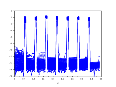
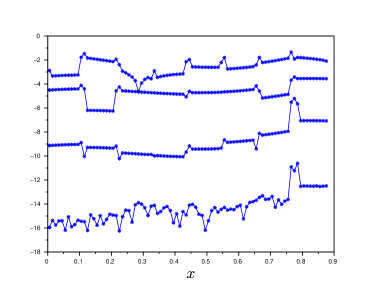
Fig. 1: Illustration of the residual when RAS is used as a nonlinear solver (left), or as a preconditioner for Newton’s method (right).

We observe that the residual of the non-linear RAS method is concentrated at the interfaces, since it must be zero inside the subdomains by construction. Thus, when Newton’s method is used to solve (6), it only needs to concentrate on reducing the residual on a small number of interface variables. This explains the fast convergence of RASPEN shown on the right of Figure 1, despite the slow convergence of the underlying RAS iteration.

Suppose we also want to include a coarse grid correction step in the Schwarz iteration (2), or equivalently in (5). Since the problem is non-linear, we need to use the Full Approximation Scheme (FAS) from multigrid to do so, see for example [3, 26]: given an approximate solution $u^{n-1}$, we compute the correction $c$ by solving the non-linear coarse problem

$${\cal L}^{c}(R_{0}u^{n-1}+c)={\cal L}^{c}(R_{0}u^{n-1})+\tilde{R}_{0}(f-{\cal L}(u^{n-1})),$$ (7)

where ${\cal L}^{c}$ is a coarse approximation of the non-linear problem (1) and $R_{0}$ is a restriction operator. This correction $c:=C_{0}(u^{n-1})$ is then added to the iterate to get the new corrected value

$$u^{n-1}_{new}=u^{n-1}+P_{0}C_{0}(u^{n-1}),$$ (8)

where $P_{0}$ is a suitable prolongation operator. Introducing this new approximation from (8) at step $n-1$ into the subdomain iteration formula (5), we obtain the method with integrated coarse correction

$$u^{n}=\sum_{i=1}^{I}{\widetilde{P}}_{i}G_{i}(u^{n-1}+P_{0}C_{0}(u^{n-1}))=:{\cal G}_{2}(u^{n-1}).$$ (9)

This stationary fixed point iteration can also be accelerated using Newton’s method: we can use Newton to solve the non-linear equation

$$\tilde{\cal F}_{2}(u):={\cal G}_{2}(u)-u=\sum_{i=1}^{I}{\widetilde{P}}_{i}G_{i}(u+P_{0}C_{0}(u))-u=0.$$ (10)

We call this method two level FAS-RASPEN.

We have written the coarse step as a correction, but not the subdomain steps. This can however also be done, by simply rewriting (5) to add and subtract the previous iterate,

$$u^{n}=\smash[t]{u^{n-1}+\sum_{i=1}^{I}{\widetilde{P}}_{i}\underbrace{(G_{i}(u^{n-1})-R_{i}u^{n-1})}_{=:C_{i}(u^{n-1})}=u^{n-1}+\sum_{i=1}^{I}{\widetilde{P}}_{i}C_{i}(u^{n-1}),}$$ (11)

where we have assumed that $\sum_{i}\tilde{P}_{i}R_{i}=I_{V}$, the identity on the vector space, see Assumption 1 in the next section. Together with the coarse grid correction (8), this iteration then becomes

$$u^{n}=\smash[t]{u^{n-1}+P_{0}C_{0}(u^{n-1})+\sum_{i=1}^{I}{\widetilde{P}}_{i}C_{i}(u^{n-1}+P_{0}C_{0}(u^{n-1})),}$$ (12)

which can be accelerated by solving with Newton the equation

$$\tilde{\cal F}_{2}(u):=P_{0}C_{0}(u)+\sum_{i=1}^{I}{\widetilde{P}}_{i}C_{i}(u+P_{0}C_{0}(u))=0.$$ (13)

This is equivalent to $\tilde{\cal F}_{2}(u)=0$ from (10), only written in correction form.

3 Definition of RASPEN and Comparison with ASPIN

We now define formally the one- and two-level versions of the RASPEN method and compare it with the respective ASPIN methods. We consider a non-linear function $F:V\rightarrow V^{\prime}$, where $V$ is a Hilbert space, and the non-linear problem of finding $u\in V$ such that

$$F(u)=0.$$ (14)

Let $V_{i},i=1,\ldots,I$ be Hilbert spaces, which would generally be subspaces of $V$. We consider for all $i=1,\ldots,I$ the linear restriction and prolongation operators $R_{i}:V\rightarrow V_{i}$, $P_{i}:V_{i}\rightarrow V$, as well as the “restricted” prolongation ${\widetilde{P}}_{i}:V_{i}\rightarrow V$.

Assumption 1.

We assume that $R_{i}$ and $P_{i}$ satisfy for $i=1,\ldots,I$

$$R_{i}P_{i}=I_{V_{i}},\quad\mbox{the identity on $V_{i}$,}$$

and that $R_{i}$ and ${\widetilde{P}}_{i}$ satisfy $\displaystyle\;\;\sum_{i=1}^{I}{\widetilde{P}}_{i}R_{i}=I_{V}.$

These are all the assumptions we need in what follows, but it is helpful to think of the restriction operators $R_{i}$ as classical selection matrices which pick unknowns corresponding to the subdomains $\Omega_{i}$, of the prolongations $P_{i}$ as $R_{i}^{T}$, and of the ${\widetilde{P}}_{i}$ as extensions based on a non-overlapping decomposition.

3.1 One- and two-level RASPEN

We can now formulate precisely the RASPEN method from the previous section: we define the local inverse $G_{i}:V\rightarrow V_{i}$ to be solutions of

$$R_{i}F\left(P_{i}G_{i}(u)+(I-P_{i}R_{i})u\right)=0.$$ (15)

In the usual PDE framework, this corresponds to solving locally on the subdomain $i$ the PDE problem on $V_{i}$ with Dirichlet boundary condition given by $u$ outside of the subdomain $i$, see (4). Then, one level RASPEN solves the non-linear equation

$$\tilde{\cal F}_{1}(u)=\sum_{i=1}^{I}{\widetilde{P}}_{i}G_{i}(u)-u=0,$$ (16)

using Newton’s method, see (6). The preconditioned nonlinear function (16) corresponds to the fixed point iteration

$$u^{n}=\smash[t]{\sum_{i=1}^{I}{\widetilde{P}}_{i}G_{i}(u^{n-1}),}$$ (17)

see (5). Equivalently, the RASPEN equation (16) can be written in correction form as

$$\tilde{\cal F}_{1}(u)=\smash[t]{\sum_{i=1}^{I}{\widetilde{P}}_{i}(G_{i}(u)-R_{i}u)=:\sum_{i=1}^{I}{\widetilde{P}}_{i}C_{i}(u),}$$ (18)

where we define the corrections $C_{i}(u):=G_{i}(u)-R_{i}u$. This way, the subdomain solves (15) can be written in terms of $C_{i}(u)$ as

$$R_{i}F(u+P_{i}C_{i}(u))=0.$$ (19)

In the special case where $F(u)=Au-b$ is affine, (19) reduces to

$$R_{i}A(u+P_{i}C_{i}(u))-R_{i}b=0\implies C_{i}(u)=A_{i}^{-1}R_{i}(b-Au),$$

where $A_{i}=R_{i}AP_{i}$ is the subdomain matrix. This implies

$$\tilde{\cal F}_{1}(u)=\sum_{i=1}^{I}{\widetilde{P}}_{i}A_{i}^{-1}R_{i}(b-Au),$$

and we immediately see that the Jacobian is the matrix $A$ preconditioned by the restricted additive Schwarz (RAS) preconditioner $\sum_{i=1}^{I}{\widetilde{P}}_{i}A_{i}^{-1}R_{i}$. Thus, if a Krylov method is used to solve the outer system, our method is equivalent to the Krylov-accelerated one-level RAS method in the linear case.

To define the two-level variant, we introduce a coarse space $V_{0}$ and the linear restriction and prolongation operators $R_{0}:V\rightarrow V_{0}$, $P_{0}:V_{0}\rightarrow V$. Let $F_{0}:V_{0}\rightarrow V^{\prime}_{0}$ be the coarse non-linear function, which could be defined by using a coarse discretization of the underlying problem, or using a Galerkin approach we use here, namely

$$F_{0}(u_{0})={\widetilde{R}}_{0}F(P_{0}(u)).$$ (20)

Here, ${\widetilde{R}}_{0}:V^{\prime}\rightarrow V^{\prime}_{0}$ is a projection operator that plays the same role as $R_{0}$, but in the residual space. In two-level FAS-RASPEN, we use the well established non-linear coarse correction $C_{0}(u)$ from the full approximation scheme already shown in (7), which in the rigorous context of this section is defined by

$$F_{0}(C_{0}(u)+R_{0}u)=F_{0}(R_{0}u)-{\widetilde{R}}_{0}F(u).$$ (21)

This coarse correction is used in a multiplicative fashion in RASPEN, i.e. we solve with Newton the preconditioned non-linear system

$$\widetilde{\cal F}_{2}(u)=P_{0}C_{0}(u)+\sum_{i=1}^{n}{\widetilde{P}}_{i}C_{i}(u+P_{0}C_{0}(u))=0.$$ (22)

This corresponds to the non-linear two-level fixed point iteration

$$u^{n+1}=u^{n}+P_{0}C_{0}(u^{n})+\sum_{i=1}^{n}{\widetilde{P}}_{i}C_{i}(u^{n}+P_{0}C_{0}(u^{n})),$$

with $C_{0}(u^{n})$ defined in (21) and $C_{i}(u^{n})$ defined in (19). This iteration is convergent, as we can see in the next section in Figure 2 in the right column. In the special case of an affine residual function $F(u)=Au-b$, a simple calculation shows that

$$\widetilde{\cal F}_{2}(u)=\left(P_{0}A_{0}^{-1}{\widetilde{R}}_{0}+\sum_{i=1}^{I}{\widetilde{P}}_{i}A_{i}^{-1}R_{i}(I_{V}-P_{0}A_{0}^{-1}{\widetilde{R}}_{0})\right)(b-Au),$$

where we assumed that the coarse function $F_{0}=A_{0}u_{0}-b_{0}$ is also linear. Thus, in the linear case, two-level RASPEN corresponds to preconditioning by a two-level RAS preconditioner, where the coarse grid correction is applied multiplicatively.

3.2 Comparison of one-level variants

In order to compare RASPEN with the existing ASPIN method, we recall the precise definition of one-level ASPIN from [8], which gives a different reformulation ${\cal F}_{1}(u)=0$ of the original equation (14) to be solved. In ASPIN, one also defines for $u\in V$ and for all $i=1,\cdots,I$ the corrections as in (19), i.e., we define $C_{i}(u)\in V_{i}$ such that

$$R_{i}F(u+P_{i}C_{i}(u))=0,$$

where $P_{i}C_{i}(u)$ are called $T_{i}$ in [8]. Then, the one-level ASPIN preconditioned function is defined by

$${\cal F}_{1}(u)=\sum_{i=1}^{I}P_{i}C_{i}(u),$$ (23)

and the preconditioned system ${\cal F}_{1}(u)=0$ is solved using a Newton algorithm with an inexact Jacobian, see Section 3.4. The ASPIN preconditioner also has a corresponding fixed point iteration: adding and subtracting $P_{i}R_{i}u$ in the definition (19) of the corrections $C_{i}$, we obtain

$$R_{i}F(u+P_{i}C_{i}(u))=R_{i}F\left(P_{i}(R_{i}u+C_{i}(u))+u-P_{i}R_{i}u\right)=0,$$

which implies, by comparing with (15) and assuming existence and uniqueness of the solution to the local problems, that

$$G_{i}(u)=R_{i}u+C_{i}(u).$$

We therefore obtain for one-level ASPIN

$${\cal F}_{1}(u)=\sum_{i=1}^{I}P_{i}C_{i}(u)=\sum_{i=1}^{I}P_{i}G_{i}(u)-\sum_{i=1}^{I}P_{i}R_{i}u,$$ (24)

which corresponds to the non-linear fixed point iteration

$$u^{n}=u^{n-1}+\sum_{i=1}^{I}P_{i}C_{i}(u^{n-1})=u^{n-1}-\sum_{i=1}^{I}P_{i}R_{i}u^{n-1}+\sum_{i=1}^{I}P_{i}G_{i}(u^{n-1}).$$ (25)

This iteration is not convergent in the overlap, already in the linear case, see [14, 20], and needs a relaxation parameter to yield convergence, see for example [12] for the non-linear case. This can be seen directly from (25): if an overlapping region belongs to $K$ subdomains, then the current iterate $u^{n}$ is subtracted $K$ times there, and then the sum of the $K$ respective subdomain solutions are added to the result. This redundancy is avoided in our formulation (17). The only interest in using an additive correction in the overlap is that in the linear case, the preconditioner remains symmetric for a symmetric problem.

We show in Figure 2 a numerical comparison of the two methods, together with Newton’s method applied directly to the non-linear problem, for the first example of the Forchheimer equation from Section 4.1 on a domain of unit size with 8 subdomains, overlap $3h$, with $h=1/100$. In these comparisons, we use ASPIN first as a fixed-point iterative solver (labelled AS for Additive Schwarz), and then as a preconditioner. We do the same for our new nonlinear iterative method, which in the figures are labelled RAS for Restricted Additive Schwarz.

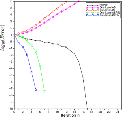
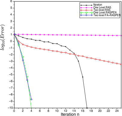
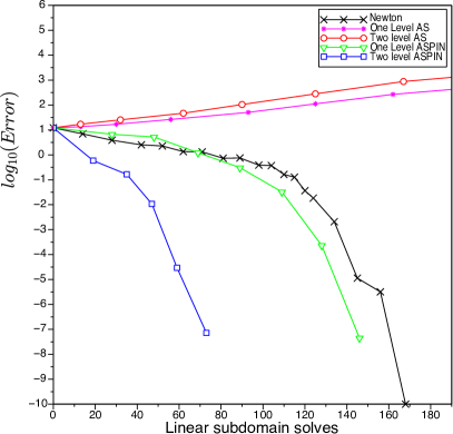
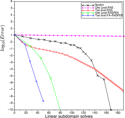
Fig. 2: Error as function of non-linear iteration numbers in the top row, and as number of subdomain solves in the bottom row, for ASPIN (left), and RASPEN (right).

We see from this numerical experiment that ASPIN as an iterative solver (AS) does not converge, whereas RASPEN used as an iterative solver (RAS) does, both with and without coarse grid. Also note that two-level RAS is faster than Newton directly applied to the non-linear problem for small iteration counts, before the superlinear convergence of Newton kicks in. The fact that RASPEN is based on a convergent iteration, but not ASPIN, has an important influence also on the Newton iterations when the methods are used as preconditioners: the ASPIN preconditioner requires more Newton iterations to converge than RASPEN does. At first sight, it might be surprising that in RASPEN, the number of Newton iterations with and without coarse grid is almost the same, while ASPIN needs more iterations without coarse grid. In contrast to the linear case with Krylov acceleration, it is not the number of Newton iterations that depends on the number of subdomains, but the number of linear inner iterations within Newton, which grows when no coarse grid is present. We show this in the second row of Figure 2, where now the error is plotted as a function of the maximum number of linear subdomain solves used in each Newton step, see Subsection 4.1.1. With this more realistic measure of work, we see that both RASPEN and ASPIN converge substantially better with a coarse grid, but RASPEN needs much fewer subdomain solves than ASPIN does.

3.3 Comparison of two-level variants

We now compare two-level FAS-RASPEN with the two-level ASPIN method of [30]. Recall that the two-level FAS-RASPEN consists of applying Newton’s method to (22),

$$\widetilde{\cal F}_{2}(u)=P_{0}C_{0}(u)+\sum_{i=1}^{n}{\widetilde{P}}_{i}C_{i}(u+P_{0}C_{0}(u))=0,$$

where the corrections $C_{0}(u)$ and $C_{i}(u)$ are defined in (21) and (19) respectively. Unlike FAS-RASPEN, two-level ASPIN requires the solution $u^{*}_{0}\in V_{0}$ to the coarse problem, i.e., $F_{0}(u^{*}_{0})=0$, which can be computed in a preprocessing step.

In two-level ASPIN, the coarse correction $C_{0}^{A}:V\rightarrow V_{0}$ is defined by

$$F_{0}(C_{0}^{A}(u)+u_{0}^{*})=-{\widetilde{R}}_{0}F(u),$$ (26)

and the associated two-level ASPIN function uses the coarse correction in an additive fashion, i.e. Newton’s method is used to solve

$${\cal F}_{2}(u)=P_{0}C_{0}^{A}(u)+\sum_{i=1}^{I}P_{i}C_{i}(u)=0,$$ (27)

with $C_{0}^{A}(u^{n})$ defined in (26) and $C_{i}(u^{n})$ defined in (19). This is in contrast to two-level FAS-RASPEN, where the coarse correction $C_{0}(u)$ is computed from the well established full approximation scheme, and is applied multiplicatively in (22). The fixed point iteration corresponding to (27) is

$$u^{n+1}=u^{n}+P_{0}C_{0}^{A}(u^{n})+\sum_{i=1}^{I}P_{i}C_{i}(u^{n}).$$

Just like its one-level counterpart, two-level ASPIN is not convergent as a fixed-point iteration without a relaxation parameter, see Figure 2 in the left column. Moreover, because the coarse correction is applied additively, the overlap between the coarse space and subdomains leads to slower convergence in the Newton solver, which does not happen with FAS-RASPEN.

3.4 Computation of Jacobian matrices

When solving (18), (22), (24) and (27) using Newton’s method, one needs to repeatedly solve linear systems involving Jacobians of the above functions. If one uses a Krylov method such as GMRES to solve these linear systems, like we do in this paper, then it suffices to have a procedure for multiplying the Jacobian with an arbitrary vector. In this section, we derive the Jacobian matrices for both one-level and two-level RASPEN in detail. We compare these expressions with ASPIN, which approximates the exact Jacobian with an inexact one in an attempt to reduce the computational cost, even though this can potentially slow down the convergence of Newton’s method. Finally, we show that this approximation is not necessary in RASPEN: in fact, all the components involved in building the exact Jacobian have already been computed elsewhere in the algorithm, so there is little additional cost in using the exact Jacobian compared with the approximate one.

3.4.1 Computation of the one-level Jacobian matrices

We now show how to compute the Jacobian matrices of ASPIN and RASPEN. To simplify notation, we define

$$u^{(i)}:=P_{i}G_{i}(u)+(I-P_{i}R_{i})u\quad\mbox{and}\quad J(v):={dF\over du}(v)$$ (28)

By differentiating (15), we obtain

$${dG_{i}\over du}(u)=-(R_{i}J(u^{(i)})P_{i})^{-1}R_{i}J(u^{(i)})+R_{i}.$$ (29)

We deduce for the Jacobian of RASPEN from (16)

$${d\tilde{\cal F}_{1}\over du}(u)=\sum_{i=1}^{I}{\widetilde{P}}_{i}{dG_{i}\over du}(u)-I=-\sum_{i=1}^{I}{\widetilde{P}}_{i}(R_{i}J(u^{(i)})P_{i})^{-1}R_{i}J(u^{(i)}),$$ (30)

since the identity cancels. Similarly, we obtain for the Jacobian of ASPEN (Additive Schwarz Preconditioned Exact Newton) in (24)

$${d{\cal F}_{1}\over du}(u)=\sum_{i=1}^{I}P_{i}{dG_{i}\over du}(u)-\sum_{i=1}^{I}P_{i}R_{i}=-\sum_{i=1}^{I}P_{i}(R_{i}J(u^{(i)})P_{i})^{-1}R_{i}J(u^{(i)}),$$ (31)

since now the terms $\sum_{i=1}^{I}P_{i}R_{i}$ cancel. In ASPIN, this exact Jacobian is replaced by the inexact Jacobian

$${d{\cal F}_{1}\over du}^{inexact}(u)=-\left(\sum_{i=1}^{I}P_{i}(R_{i}J(u)P_{i})^{-1}R_{i}\right)J(u).$$

We see that this is equivalent to preconditioning the Jacobian $J(u)$ of $F(u)$ by the additive Schwarz preconditioner, up to the minus sign. This can be convenient if one has already a code for this, as it was noted in [8]. The exact Jacobian is however also easily accessible, since the Newton solver for the non-linear subdomain system $R_{i}F\left(P_{i}G_{i}(u)+(I-P_{i}R_{i})u\right)=0$ already computes and factorizes the local Jacobian matrix $R_{i}J(u^{(i)})P_{i}$. Therefore, the only missing ingredient for computing the exact Jacobian of ${\cal F}_{1}$ is the matrices $R_{i}J(u^{(i)})$, which only differ from $R_{i}J(u^{(i)})P_{i}$ by a few additional columns, corresponding in the usual PDEs framework to the derivative with respect to the Dirichlet boundary conditions. In contrast, the computation of the inexact ASPIN Jacobian requires one to recompute the entire Jacobian of $F(u)$ after the subdomain non-linear solves.

3.4.2 Computation of the two-level Jacobian matrices

We now compare the Jacobians for the two-level variants. For RASPEN, we need to differentiate $\tilde{\cal F}_{2}$ with respect to $u$, where $\tilde{\cal F}_{2}$ is defined in (22):

$$\widetilde{\cal F}_{2}(u)=P_{0}C_{0}(u)+\sum_{i=1}^{n}{\widetilde{P}}_{i}C_{i}(u+P_{0}C_{0}(u)).$$

To do so, we need $\frac{dC_{0}}{du}$ and $\frac{dC_{i}}{du}$ for $i=1,\ldots,I$. The former can be obtained by differentiating (21):

$$F_{0}^{\prime}(R_{0}u+C_{0}(u))\left(R_{0}+\frac{dC_{0}}{du}\right)=F_{0}^{\prime}(R_{0}u)R_{0}-{\widetilde{R}}_{0}F^{\prime}(u).$$

Thus, we have

$$\frac{dC_{0}}{du}=-R_{0}+\hat{J}_{0}^{-1}(J_{0}R_{0}-{\widetilde{R}}_{0}J(u)),$$ (32)

where $J_{0}=F_{0}^{\prime}(R_{0}u)$ and $\hat{J}_{0}=F_{0}^{\prime}(R_{0}u+C_{0}(u))$. Note that the two Jacobian matrices are evaluated at different arguments, so no cancellation is possible in (32) except in special cases (e.g., if $F_{0}$ is an affine function). Nonetheless, they are readily available: $\hat{J}_{0}$ is simply the Jacobian for the non-linear coarse solve, so it would have already been calculated and factorized by Newton’s method. $J_{0}$ would also have been calculated during the coarse Newton iteration if $R_{0}u$ is used as the initial guess.

We also need $\frac{dC_{i}}{du}$ from the subdomain solves. From the relation $G_{i}(u)=R_{i}u+C_{i}(u),$ we deduce immediately from (29) that

$$\frac{dC_{i}}{du}=\frac{dG_{i}}{du}-R_{i}=-(R_{i}J(u^{(i)})P_{i})^{-1}R_{i}J(u^{(i)}),$$ (33)

where $u^{(i)}=u+P_{i}C_{i}(u).$ Thus, the Jacobian for the two-level RASPEN function is

$$\frac{d\widetilde{\mathcal{F}}_{2}}{du}=P_{0}\frac{dC_{0}}{du}-\sum_{i}\tilde{P}_{i}(R_{i}J(v^{(i)})P_{i})^{-1}R_{i}J(v^{(i)})\left(I+P_{0}\frac{dC_{0}}{du}\right),$$ (34)

where $\frac{dC_{0}}{du}$ is given by (32) and $v^{(i)}=u+P_{0}C_{0}(u)+P_{i}C_{i}(u+P_{0}C_{0}(u)).$

For completeness, we compute the Jacobian for two-level ASPIN. First, we obtain $\frac{dC_{0}^{A}}{du}$ by differentiating (26), which gives

$$\frac{dC_{0}^{A}}{du}=-\hat{J}_{0}^{-1}{\widetilde{R}}_{0}J(u),$$ (35)

where $\hat{J}_{0}=F_{0}^{\prime}(C_{0}^{A}(u)+u_{0}^{*}).$ In addition, two-level ASPIN uses as approximation for (33)

$$\frac{dC_{i}}{du}\approx-(R_{i}J(u)P_{i})^{-1}R_{i}J(u).$$ (36)

Thus, the inexact Jacobian for the two-level ASPIN function is

$$\frac{d\mathcal{F}_{2}}{du}\approx-P_{0}\hat{J}_{0}^{-1}{\widetilde{R}}_{0}J(u)-\sum_{i}P_{i}(R_{i}J(u)P_{i})^{-1}R_{i}J(u).$$ (37)

Comparing (34) with (37), we see two major differences. First, $dC_{0}/du$ only simplifies to $-{\widetilde{R}}_{0}J(u)$ if $J_{0}=\hat{J}_{0}$, i.e., if $F_{0}$ is affine. Second, (34) resembles a two-stage multiplicative preconditioner, whereas (37) is of the additive type. This is due to the fact that the coarse correction in two-level RASPEN is applied multiplicatively, whereas two-level ASPIN uses an additive correction.

4 Numerical experiments

In this section, we compare the new non-linear preconditioner RASPEN to ASPIN for the Forchheimer model, which generalizes the linear Darcy model in porous media flow [18, 33, 10], and for a 2D non-linear diffusion problem that appears in [1].

4.1 Forchheimer model and discretization

Let us consider the Forchheimer parameter $\beta>0$, the permeability $\lambda\in L^{\infty}(\Omega)$ such that $0<\lambda_{min}\leq\lambda(x)\leq\lambda_{max}$ for all $x\in\Omega$, and the function $q(g)=\mbox{sgn}(g){-1+\sqrt{1+4\beta|g|}\over 2\beta}$. The Forchheimer model on the interval $\Omega=(0,L)$ is defined by the equation

$$\left\{\begin{array}[]{rcll}\left(q(-\lambda(x)u(x)^{\prime})\right)^{\prime}&=&f(x)&\mbox{ in }\Omega,\\ u(0)&=&u^{D}_{0},\\ u(L)&=&u^{D}_{L}.\end{array}\right.$$ (38)

Note that at the limit when $\beta\rightarrow 0^{+}$, we recover the linear Darcy equation. We consider a 1D mesh defined by the $M+1$ points

$$0=x_{1\over 2}<\cdots<x_{K+{1\over 2}}<\cdots<x_{M+{1\over 2}}=L.$$

The cells are defined by $K=(x_{K-{1\over 2}},x_{K+{1\over 2}})$ for $K\in{\cal M}=\{1,\cdots,M\}$ and their center by $x_{K}={x_{K-{1\over 2}}+x_{K+{1\over 2}}\over 2}$. The Forchheimer model (38) is discretized using a Two Point Flux Approximation (TPFA) finite volume scheme. We define the TPFA transmissibilities by

$$\left\{\begin{array}[]{r@{\,\,}c@{\,\,}l}&&\displaystyle T_{K+{1\over 2}}={1\over{|x_{K+{1\over 2}}-x_{K}|\over\lambda_{K}}+{|x_{K+1}-x_{K+{1\over 2}}|\over\lambda_{K+1}}}\mbox{ for }K=1,\cdots,M-1\\ &&\displaystyle T_{1\over 2}={\lambda_{1}\over|x_{1}-x_{1\over 2}|},\quad\displaystyle T_{M+{1\over 2}}={\lambda_{M}\over|x_{M+{1\over 2}}-x_{M}|},\end{array}\right.$$

with $\lambda_{K}={1\over|x_{K+{1\over 2}}-x_{K-{1\over 2}}|}\int_{x_{K-{1\over 2}}}^{x_{K+{1\over 2}}}\lambda(x)dx$. Then, the $M$ cell unknowns $u_{K}$, $K\in{\cal M}$, are the solution of the set of $M$ conservation equations

$$\left\{\begin{array}[]{r@{\,\,}c@{\,\,}l}\displaystyle q(T_{K+{1\over 2}}(u_{K}-u_{K+1}))+q(T_{K-{1\over 2}}(u_{K}-u_{K-1}))&=&f_{K},\,K=2,\cdots,M-1\\ \displaystyle q(T_{{3\over 2}}(u_{1}-u_{2}))+q(T_{{1\over 2}}(u_{1}-u_{0}^{D}))&=&f_{1},\\ \displaystyle q(T_{M+{1\over 2}}(u_{M}-u_{L}^{D}))+q(T_{M-{1\over 2}}(u_{M}-u_{M-1}))&=&f_{M},\end{array}\right.$$

with $f_{K}=\int_{x_{K-{1\over 2}}}^{x_{K+{1\over 2}}}f(x)dx$. In the following numerical tests we will consider a uniform mesh of cell size denoted by $h={L\over M}$.

4.1.1 One level variants

We start from a non-overlapping decomposition of the set of cells

$$\widetilde{\cal M}_{i},i=1,\cdots,I,$$

such that ${\cal M}=\bigcup_{i=1,\cdots,I}\widetilde{\cal M}_{i}$ and $\widetilde{\cal M}_{i}\cap\widetilde{\cal M}_{j}=\emptyset$ for all $i\neq j$.

The overlapping decomposition ${\cal M}_{i},i=1,\cdots,I$ of the set of cells is obtained by adding $k$ layers of cells to each $\widetilde{\cal M}_{i}$ to generate overlap with the two neighbouring subdomains $\widetilde{\cal M}_{i-1}$ (if $i>1$) and $\widetilde{\cal M}_{i+1}$ (if $i<I$) in the simple case of our one dimensional domain.

In the ASPIN framework, we set $V={\mathbb{R}}^{\#{\cal M}}$, and $V_{i}={\mathbb{R}}^{\#{\cal M}_{i}}$, $i=1,\cdots,I$. The restriction operators are then defined by

$$(R_{i}v)_{K}=v_{K}\mbox{ for }K\in{\cal M}_{i},$$

and the prolongation operators are

$$\left\{\begin{array}[]{r@{\,\,}c@{\,\,}l}(P_{i}v_{i})_{K}&=&v_{K}\mbox{ for }K\in{\cal M}_{i},\\ (P_{i}v_{i})_{K}&=&0\mbox{ for }K\not\in{\cal M}_{i},\end{array}\right.\quad\text{ and }\quad\left\{\begin{array}[]{r@{\,\,}c@{\,\,}l}({\widetilde{P}}_{i}v_{i})_{K}&=&v_{K}\mbox{ for }K\in\widetilde{\cal M}_{i},\\ ({\widetilde{P}}_{i}v_{i})_{K}&=&0\mbox{ for }K\not\in\widetilde{\cal M}_{i}.\end{array}\right.$$

The coarse grid is obtained by the agglomeration of the cells in each $\widetilde{\cal M}_{i}$ defining a coarse mesh of $(0,L)$.

Finally, we set $V_{0}={\mathbb{R}}^{I}$. In the finite volume framework, we define for all $v\in V$

$$(R_{0}v)_{i} ={1\over\#\widetilde{M}_{i}}\sum_{K\in\widetilde{\cal M}_{i}}v_{K}\quad\mbox{for all }i=1,\cdots,I,$$

$$({\widetilde{R}}_{0}v)_{i} =\sum_{K\in\widetilde{\cal M}_{i}}v_{K}\;\;\quad\qquad\mbox{for all }i=1,\cdots,I.$$

In our case of a uniform mesh, $R_{0}$ corresponds to the mean value in the coarse cell $i$ for cellwise constant functions on ${\cal M}$, whereas ${\widetilde{R}}_{0}$ corresponds to the aggregate flux over the coarse cell ${\widetilde{\cal M}}_{i}$.

For $v_{0}\in V_{0}$, its prolongation $v=P_{0}v_{0}\in V$ is obtained by the piecewise linear interpolation $\varphi(x)$ on $(0,x_{1})$, $(x_{1},x_{2}),\cdots,(x_{I},L)$ where the $x_{i}$ are the centers of the coarse cells, and $\varphi(x_{i})=(v_{0})_{i}$, $i=1,\cdots,I$, $\varphi(0)=0$, $\varphi(L)=0$. Then, $v=P_{0}v_{0}$ is defined by $v_{K}=\varphi(x_{K})$ for all $K\in{\cal M}$. The coarse grid operator $F_{0}$ is defined by $F_{0}(v_{0})={\widetilde{R}}_{0}F(P_{0}v_{0})$ for all $v_{0}\in V_{0}$.

We use for the numerical tests the domain $\Omega=(0,3/2)$ with the boundary conditions $u(0)=0$ and $u({3/2})=1$, and different values of $\beta$. As a first challenging test, we choose the highly variable permeability field $\lambda$ and the oscillating right hand side shown in Figure 3.

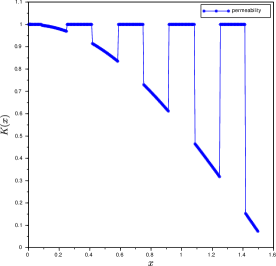
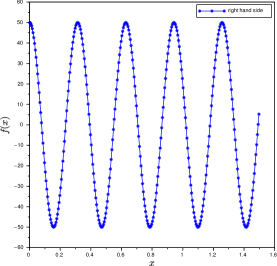
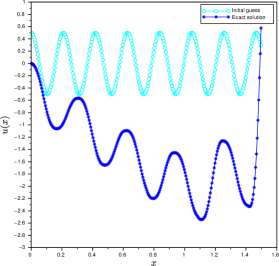
Fig. 3: Permeability field (left), source term (middle), initial guess and solution (right).

We measure the relative $l^{1}$ norms of the error obtained at each Newton iteration as a function of the parallel linear solves $LS_{n}$ needed in the subdomains per Newton iteration, which is a realistic measure for the cost of the method. Each Newton iteration requires two major steps:

1. the evaluation of the fixed point function ${\cal F}$, which means solving a non-linear problem in each subdomain. This is done using Newton in an inner iteration on each subdomain, and thus requires at each inner iteration a linear subdomain solve performed in parallel by all subdomains (we have used a sparse direct solver for the linear subdomain solves in our experiments, but one can also use an iterative method if good preconditioners are available). We denote the maximum number of inner iterations needed by the subdomains at the outer iteration $j$ by $ls_{j}^{in}$, and it is the maximum which is relevant, because if other subdomains finish earlier, they still have to wait for the last one to finish.

2. the Jacobian matrix needs to be inverted, which we do by GMRES, and each GMRES iteration will also need a linear subdomain solve per subdomain. We denote the number of linear solves needed by GMRES at the outer Newton iteration step $j$ by $ls_{j}^{G}$.

Hence, the number of linear subdomain solves for the outer Newton iteration $j$ to complete is $ls_{j}^{in}+ls_{j}^{G}$, and the total number of linear subdomain solves after $n$ outer Newton iterations is $LS_{n}:=\sum_{j=1}^{n}\left(ls_{j}^{in}+ls_{j}^{G}\right)$. In all the numerical tests, we stop the linear GMRES iterations when the relative residual falls below $10^{-8}$, and the tolerances for the inner and outer Newton iterations are also set to $10^{-8}$. Adaptive tolerances could certainly lead to more savings [15, 16], but our purpose here is to compare the non-linear preconditioners in a fixed setting. The initial guess we use in all our experiments is shown in Figure 3 on the right, together with the solution.

We show in Figure 5

                 

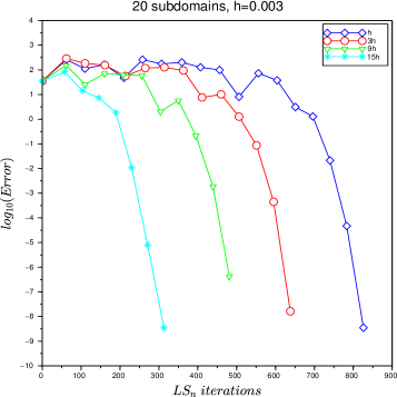
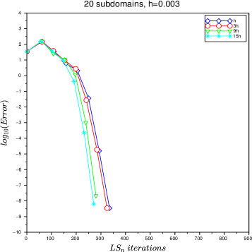
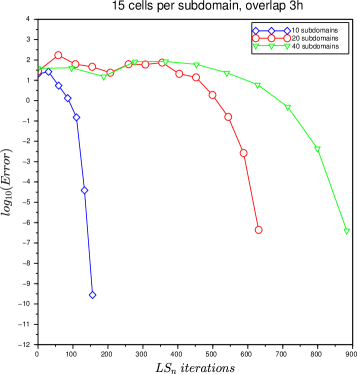
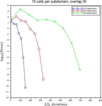
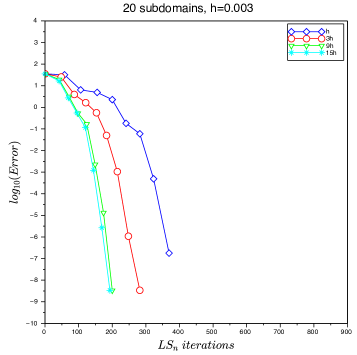
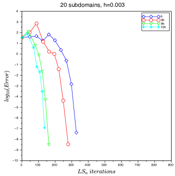
Fig. 4: Error obtained with one-level ASPIN (left) and one-level RASPEN (right): in the top row obtained with $20$ subdomains, $h=0.003$, and decreasing size of overlap $15h$, $9h$, $3h$, $h$; in the bottom row obtained with different number of subdomains $10,20$ and $40$, overlap $3h$, and a fixed number of cells per subdomain. The Forchheimer problem is defined by the permeability, source term, solution and initial guess of Figure 3.

Fig. 5: Error obtained with two-level ASPIN (left) and two-level FAS RASPEN (right) obtained with $20$ subdomains, $h=0.003$, and decreasing overlap $15h$, $9h$, $3h$, $h$. The Forchheimer problem is defined by the permeability, source term, solution and initial guess of Figure 3.

how the convergence depends on the overlap and the number of subdomains for one level ASPIN and RASPEN with Forchheimer model parameter $\beta=1$. In the top row on the left of Figure 5, we see that for ASPIN the number of linear iterations increases much more rapidly when decreasing the overlap than for RASPEN on the right for a fixed mesh size $h=0.003$ and number of subdmains equal $20$. In the bottom row of Figure 5, we see that the convergence of both one level ASPIN and RASPEN depends on the number of subdomains, but RASPEN seems to be less sensitive than ASPIN.

4.1.2 Two level variants

In Figure 5, we show the dependence of two-level ASPIN and two-level FAS-RASPEN on a decreasing size of the overlap, as we did for the one-level variants in the top row of Figure 5. We see that the addition of the coarse level improves the performance, for RASPEN when the overlap is large, and in all cases for ASPIN.

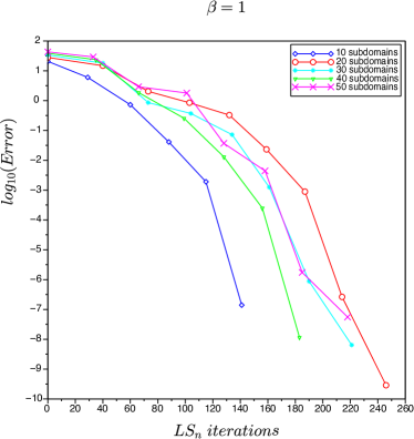
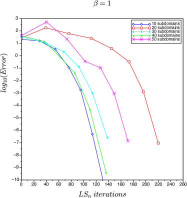
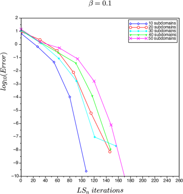
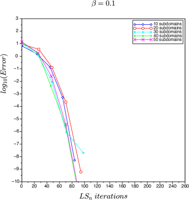
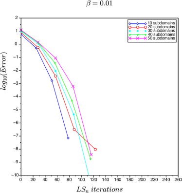
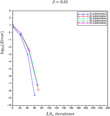
Fig. 6: Error obtained with two-level ASPIN (left) and two-level FAS RASPEN (right) and different number of subdomains $10,20,30,40,50$. From top to bottom with decreasing Forchheimer parameter $\beta=1,0.1,0.01$. The Forchheimer problem is defined by the permeability, source term, solution and initial guess of Figure 3.

ASPIN
Number of subdomains	10		20		40
	PIN iter.	$LS_{n}$ iter.	PIN iter.	$LS_{n}$ iter.	PIN iter.	$LS_{n}$ iter.
h	8	184	15	663	-	-
3h	7	156	14	631	11	883
5h	6	130	11	479	10	744
RASPEN
Number of subdomains	10		20		40
	PEN iter.	$LS_{n}$ iter.	PEN iter.	$LS_{n}$ iter.	PEN iter.	$LS_{n}$ iter.
h	7	150	9	369	9	701
3h	7	145	8	324	9	691
5h	6	126	7	274	9	659
Two-level ASPIN
Number of subdomains	10		20		40
	PIN iter.	$LS_{n}$ iter.	PIN iter.	$LS_{n}$ iter.	PIN iter.	$LS_{n}$ iter.
h	7	184	9	316	8	285
3h	6	141	9	246	7	183
5h	6	135	8	199	7	164
Two-level FAS-RASPEN
Number of subdomains	10		20		40
	PEN iter.	$LS_{n}$ iter.	PEN iter.	$LS_{n}$ iter.	PEN iter.	$LS_{n}$ iter.
h	7	134	9	272	8	258
3h	7	133	8	220	6	136
5h	6	112	8	211	6	116

Table 1: Comparison in terms of non-linear and linear iterations of the different algorithms for the Forchheimer problem defined by the permeability, source term, solution and initial guess of Figure 3.

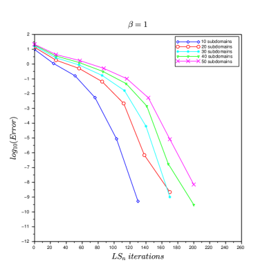
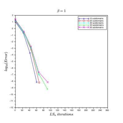
Fig. 7: Error obtained with two-level ASPIN (left) and two-level FAS RASPEN (right) with overlap $3h$, and different number of subdomains $10,20,30,40,50$ for the smooth Forchheimer example.

ASPIN
Number of subdomains	10		20		40
	PIN iter.	$LS_{n}$ iter.	PIN iter.	$LS_{n}$ iter.	PIN iter.	$LS_{n}$ iter.
h	5	118	5	228	6	520
3h	5	118	5	227	6	516
5h	5	117	5	222	6	480
RASPEN
Number of subdomains	10		20		40
	PEN iter.	$LS_{n}$ iter.	PEN iter.	$LS_{n}$ iter.	PEN iter.	$LS_{n}$ iter.
h	4	92	4	172	4	340
3h	4	87	4	172	4	331
5h	4	88	4	168	4	313
Two level ASPIN
Number of subdomains	10		20		40
	PIN iter.	$LS_{n}$ iter.	PIN iter.	$LS_{n}$ iter.	PIN iter.	$LS_{n}$ iter.
h	5	140	5	240	5	280
3h	5	130	6	170	6	200
5h	5	115	7	149	6	147
Two level FAS RASPEN
Number of subdomains	10		20		40
	PEN iter.	$LS_{n}$ iter.	PEN iter.	$LS_{n}$ iter.	PEN iter.	$LS_{n}$ iter.
h	4	77	3	87	4	131
3h	3	60	3	67	4	90
5h	3	55	3	57	3	57

Table 2: Comparison in terms of non-linear and linear iterations of the different algorithms for the smooth Forchheimer example.

Number of		1-Level				2-Level
subdomains	$n$	$ls_{n}^{G}$	$ls_{n}^{in}$	$ls_{n}^{\min}$	$LS_{n}$	$ls_{n}^{G}$	$ls_{n}^{in}$	$ls_{n}^{\min}$	$LS_{n}$
$10$	1	19 (20)	4 (4)	3 (3)		15 (20)	7 (4)	3 (3)
	2	19 (20)	3 (6)	3( 3)	87 (118)	16 (21)	3 (6)	2 (3)	60 (130)
	3	19 (20)	2 (4)	2 (2)		17 (22)	2 (3)	1 (2)
	4	19 (20)	2 (2)	1 (2)		- (24)	- (3)	- (1)
	5	- (21)	- (1)	- (1)		- (25)	- (2)	- (1)
$20$	1	40 (41)	5 (5)	3 (3)		15 (22)	8 (5)	3 (3)
	2	40 (41)	3 (7)	2 (2)	172 (227)	18 (23)	3 (6)	2 (3)	67 (170)
	3	40 (41)	2 (5)	1 (2)		21 (24)	2 (5)	1 (2)
	4	40 (41)	2 (3)	1 (1)		- (24)	- (3)	- (1)
	5	- (41)	- (2)	- (1)		- (24)	- (2)	- (1)
	6	- (-)	- (-)	- (-)		- (31)	- (1)	- (1)
$40$	1	78 (80)	5 (5)	3 (3)		14 (22)	9 (5)	3 (3)
	2	81 (81)	3 (6)	2 (2)	331 (516)	17 (22)	3 (7)	1 (2)	90 (200)
	3	79 (82)	2 (6)	1 (2)		20 (24)	2 (6)	1 (2)
	4	81 (82)	2 (5)	1 (1)		24 (24)	1(5)	0 (1)
	5	- (82)	- (3)	- (1)		- (23)	- (3)	- (1)
	6	- (82)	- (2)	- (1)		- (25)	- (2)	- (1)
	7	- (-)	- (-)	- (-)		- (31)	- (1)	- (0)

Table 3: Numerical results with one- and two-level RASPEN and ASPIN for the 1D non-linear smooth Forchheimer problem. ‘-’ indicates that the method has converged.

In Figure 6, we present a study of the influence of the number of subdomains on the convergence for two-level ASPIN and two-level FAS-RASPEN with different values of the Forchheimer parameter $\beta=1,0.1,0.01$ which governs the non-linearity of the model (the model becomes linear for $\beta=0$). An interesting observation is that for $\beta=1$, the convergence of both two-level ASPIN and two-level FAS-RASPEN depends on the number of subdomains in an irregular fashion: increasing the number of subdomains sometimes increases iteration counts, and then decreases them again. We will study this effect further below, but note already from Figure 6 that this dependence disappears for two-level FAS-RAPSEN as the the nonlinearity diminishes (i.e., as $\beta$ decreases), and is weakened for two-level ASPIN.

We finally show in Table 1 the number of outer Newton iterations (PIN iter for ASPIN and PEN iter for RASPEN) and the total number of linear iterations ($LS_{n}$ iter) for various numbers of subdomains and various overlap sizes obtained with ASPIN, RASPEN, two-level ASPIN and two-level FAS-RASPEN. We see that the coarse grid considerably improves the convergence of both RASPEN and ASPIN. Also, in all cases, RASPEN needs substantially fewer linear iterations than ASPIN.

We now return to the irregular number of iterations observed in Figure 6 for the Forchheimer parameter $\beta=1$, i.e when the non-linearity is strong. We claim that this irregular dependence is due to strong variations in the initial guesses used by RASPEN and ASPIN at subdomain interfaces, which is in turn caused by the highly variable contrast and oscillating source term we used, leading to an oscillatory solution, see Figure 3. In other words, we expect the irregularity to disappear when the solution is non-oscillatory. To test this, we now present numerical results with the less variable permeability function $\lambda(x)=\cos(x)$ and source term $f(x)=\cos(x)$ as well, which leads to a smooth solution. Starting with a zero initial guess, we show in Figure 7 the results obtained for Forchheimer parameter $\beta=1$, corresponding to the first row of Figure 6.

We clearly see that the irregular behavior has now disappeared for both two-level ASPIN and RASPEN, but two-level ASPIN still shows some dependence of the iteration numbers as the number of subdomains increases. We show in Table 2 the complete results for this smoother example, and we see that the irregular convergence behavior of the two-level methods is no longer present. We finally give in Table 3 a detailed account of the linear subdomain solves needed for each outer Newton iteration $n$ for the case of an overlap of $3h$. There, we use the format $it_{\mathrm{RASPEN}}(it_{\mathrm{ASPIN}})$, where $it_{\mathrm{RASPEN}}$ is the iteration count for RASPEN and $it_{\mathrm{ASPIN}}$ is the iteration count for ASPIN. We show in the first column the linear subdomain solves $ls_{n}^{G}$ required for the inversion of the Jacobian matrix using GMRES, see item 2 in Subsection 4.1.1, and in the next column the maximum number of iterations $ls_{n}^{in}$ needed to evaluate the nonlinear fixed point function ${\cal F}$, see item 1 in Subsection 4.1.1. In the next column, we show for completeness also the smallest number of inner iterations $ls_{n}^{\min}$ any of the subdomains needed, to illustrate how balanced the work is in this example. The last column then contains the total number of linear iterations $LS_{n}$, see Subsection 4.1.1. These results show that the main gain of RASPEN is a reduced number of Newton iterations, i.e. it is a better non-linear preconditioner than ASPIN, and also a reduced number of inner iterations for the non-linear subdomain solves, i.e. the preconditioner is less expensive. This leads to the substantial savings observed in the last columns, and in Table 2.

4.2 A non-linear Poisson problem

We now test the non-linear preconditioners on the two dimensional non-linear diffusion problem (see [1])

$$\left\{\begin{array}[]{rcll}-\nabla\cdot((1+u^{2})\nabla u)&=&f,&\Omega=[0,1]^{2},\\ u&=&1,&x=1,\\ \displaystyle\frac{\partial u}{\partial\mathbf{n}}&=&0,&\mbox{otherwise.}\end{array}\right.$$ (39)

The isovalues of the exact solution are shown in Figure 8. To calculate this solution, we use a discretization with P1 finite elements on a uniform triangular mesh. All calculations have been performed using FreeFEM++, a C++ based domain-specific language for the numerical solution of PDEs using finite element methods [25]. We consider a decomposition of the domain into $N\times N$ subdomains with an overlap of one mesh size $h$, and we keep the number of degrees of freedom per subdomain fixed in our experiments. We show in Table 4 a detailed account of the number of linear subdomain solves needed for RASPEN and ASPIN at each outer Newton iteration $n$, using the same notation as in Table 3 (Newton converged in three iterations for all examples to a tolerance of $10^{-8}$). We see from these experiments that RASPEN, which is a non-linear preconditioner based on a convergent underlying fixed point iteration, clearly outperforms ASPIN, which would not be convergent as a basic fixed point iteration.

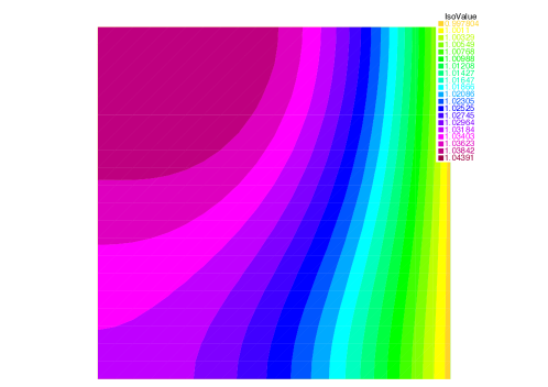
Fig. 8: Exact solution of the non-linear Poisson problem (39)

		1-Level				2-Level
$N\times N$	$n$	$ls_{n}^{G}$	$ls_{n}^{in}$	$ls_{n}^{\min}$	$LS_{n}$	$ls_{n}^{G}$	$ls_{n}^{in}$	$ls_{n}^{\min}$	$LS_{n}$
$2\times 2$	1	15(20)	4(4)	3(3)		13(23)	4(4)	3(3)
	2	17(23)	3(3)	3(3)	59(78)	15(26)	3(3)	3(3)	54(86)
	3	18(26)	2(2)	2(2)		17(28)	2(2)	2(2)
$4\times 4$	1	32(37)	3(3)	3(3)		18(33)	3(3)	3(3)
	2	35(41)	3(3)	2(2)	113(132)	22(39)	3(3)	2(2)	74(126)
	3	38(46)	2(2)	2(2)		26(46)	2(2)	2(2)
$8\times 8$	1	62(71)	3(3)	2(2)		18(35)	3(3)	3(2)
	2	67(77)	3(3)	2(2)	211(240)	23(44)	3(3)	2(2)	77(139)
	3	74(84)	2(2)	1(2)		28(53)	2(2)	2(1)
$16\times 16$	1	125(141)	3(3)	2(2)		18(35)	3(3)	3(2)
	2	136(155)	2(2)	2(2)	418(471)	23(44)	2(2)	2(2)	75(140)
	3	150(167)	2(2)	1(1)		27(54)	2(2)	2(1)

Table 4: Numerical results with one- and two-level RASPEN and ASPIN for the non-linear diffusion problem.

4.3 A problem with discontinuous coefficients

We now test the non-linear preconditioners on the two dimensional Forchheimer problem, which can be written as

$$\left\{\begin{gathered}-\nabla\cdot{\bf q}=0,\qquad\Omega=[0,1]^{2},\\ {\bf q}+\beta|{\bf q}|{\bf q}=\Lambda({\bf x})\nabla u,\\ u=0\quad\text{on $\Gamma_{d0}$},\qquad u=1\quad\text{on $\Gamma_{d1}$},\\ {\bf q}\cdot{\bf n}=0\quad\text{on $\partial\Omega\setminus(\Gamma_{d0}\cup\gamma_{d1})$,}\end{gathered}\right.$$ (40)

where the Dirichlet boundaries $\Gamma_{d0}$ and $\Gamma_{d1}$ are located at the bottom left and top right corners of the domain, namely,

$$\Gamma_{d0}=\{(x,y)\in\partial\Omega:x+y<0.2\},\qquad\Gamma_{d1}=\{(x,y)\in\partial\Omega:x+y>1.8\}.$$

The permeability $\Lambda({\bf x})$ is equal to 1000 everywhere except at the two inclusions shown in red and black in the left panel of Figure 9, where it is equal to 1. The mesh in the above figure is used to discretize the problem, using P1 finite elements; the exact solution is shown in the right panel.

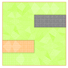
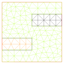
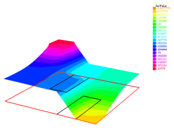
Fig. 9: Left: Fine discretization of the domain for $N=4$. The red and black inclusions correspond to low-permeability regions. Middle: Coarse grid used for two-level methods. Right: Exact solution for the 2D Forchheimer problem.

	$\beta=0.1$			$\beta=1$
	$2\times 2$	$4\times 4$	$8\times 8$	$2\times 2$	$4\times 4$	$8\times 8$
Newton	19	19	19	38	44	48
ASPIN	6	div.	div.	6	div.	div.
ASPIN2	5	6	7	6	7	9
RASPEN	5	4	4	5	5	5
RASPEN2	4	4	4	5	5	6

Table 5: Number of non-linear iterations required for convergence by various algorithms for the 2D Forchheimer problem, as a function of problem size. Divergence of the method is indicated by ‘div’.

			1-Level				2-Level
$N\times N$	$\beta$	$n$	$ls_{n}^{G}$	$ls_{n}^{in}$	$ls_{n}^{\min}$	$LS_{n}$	$ls_{n}^{G}$	$ls_{n}^{in}$	$ls_{n}^{\min}$	$LS_{n}$
$2\times 2$	0.1	1	22(29)	5(5)	5(5)	82(106)	10(20)	6(5)	5(5)	47(102)
		2	24(32)	4(4)	4(4)		12(21)	3(4)	3(4)
		3	25(33)	2(3)	2(2)		14(22)	2(3)	2(3)
		4	- (-)	- (-)	- (-)		- (25)	- (2)	- (2)
	0.2	1	22(28)	4(4)	3(3)	53(69)	9(19)	4(4)	3(3)	29(49)
		2	24(34)	3(3)	3(3)		14(23)	2(3)	2(3)
	0.5	1	22(28)	4(4)	4(4)	53(69)	9(19)	4(4)	3(3)	29(49)
		2	24(34)	3(3)	3(3)		14(23)	2(3)	2(3)
	1.0	1	22(28)	4(4)	4(4)	53(69)	10(21)	4(4)	3(3)	30(51)
		2	24(34)	3(3)	2(2)		14(23)	2(3)	2(2)
$4\times 4$	0.1	1	41(53)	5(5)	4(4)	145(179)	11(21)	6(6)	4(4)	52(111)
		2	45(56)	4(4)	3(3)		14(23)	3(4)	3(3)
		3	48(58)	2(3)	2(2)		16(24)	2(4)	2(3)
		4	- (-)	- (-)	- (-)		- (26)	- (3)	- (2)
	0.2	1	41(52)	4(4)	3(3)	94(118)	11(21)	4(4)	3(3)	33(54)
		2	47(59)	2(3)	2(2)		16(26)	2(3)	2(2)
	0.5	1	41(51)	4(4)	3(3)	94(116)	11(21)	4(4)	3(3)	33(54)
		2	47(58)	2(3)	2(2)		16(26)	2(3)	2(2)
	1.0	1	41(51)	4(4)	3(3)	94(116)	11(21)	4(3)	3(3)	34(53)
		2	47(58)	2(3)	2(2)		17(26)	2(3)	2(2)
$8\times 8$	0.1	1	86(104)	5(5)	3(3)	468(573)	16(24)	6(5)	3(3)	73(160)
		2	92(111)	3(4)	2(2)		21(27)	4(4)	3(3)
		3	95(115)	3(3)	2(2)		24(26)	2(4)	2(2)
		4	90(116)	2(2)	1(1)		- (30)	- (3)	- (2)
		5	90(111)	2(2)	1(1)		- (35)	- (2)	- (1)
	0.2	1	84(103)	4(4)	3(3)	373(457)	16(24)	4(4)	3(3)	46(62)
		2	93(115)	3(3)	2(2)		24(31)	2(3)	2(2)
		3	94(117)	2(2)	1(1)		- (-)	- (-)	- (-)
		4	91(111)	2(2)	1(1)		- (-)	- (-)	- (-)
	0.5	1	84(104)	4(4)	3(3)	374(461)	16(25)	4(4)	3(3)	46(63)
		2	94(115)	3(3)	2(2)		24(31)	2(3)	2(2)
		3	94(119)	2(2)	1(1)		- (-)	- (-)	- (-)
		4	91(112)	2(2)	1(1)		- (-)	- (-)	- (-)
	1.0	1	84(104)	4(4)	2(2)	375(461)	16(25)	4(4)	3(2)	47(64)
		2	95(115)	3(3)	2(2)		25(32)	2(3)	2(2)
		3	95(119)	2(2)	1(1)		- (-)	- (-)	- (-)
		4	91(112)	2(2)	1(1)		- (-)	- (-)	- (-)

Table 6: Numerical results with one- and two-level RASPEN and ASPIN for the 2D Forchheimer problem. ‘-’ indicates that the method has converged.

We consider a decomposition of the domain into $N\times N$ subdomains with an overlap of one mesh size $h$, and we keep the number of degrees of freedom per subdomain fixed in our experiments. For the two-level methods, the coarse function $F_{0}$ consists of a P1 discretization of the problem over the coarse grid shown in the middle panel of Figure 9.

To measure the difficulty of this problem, we run our non-linear algorithms (standard Newton, one and two-level ASPIN, one and two-level RASPEN) on this problem for $\beta=0.1$ and $\beta=1$. We show in Table 5 the number of iterations required for the convergence of each algorithm. We see that between the discontinuous permeability and the non-linearity introduced by $\beta$, standard Newton requires many iterations to converge, and one-level ASPIN diverges for the larger problems. On the other hand, one and two-level RASPEN (and two-level ASPIN, to a lesser extent) converge in a small number of non-linear iterations.

Next, we compare the one and two-level variants of ASPIN and RASPEN in terms of the total amount of computational work. To deal with the convergence problem in one-level ASPIN, we adopt the continuation approach, where we solve the problem for a sequence of $\beta$ (0, 0.1, 0.2, 0.5 and 1.0), using the solution for the previous $\beta$ as the initial guess for the next one. Table 6 shows a detailed account for each outer Newton iteration $n$ of the linear subdomain solves needed for both RASPEN and ASPIN using the same notation as in Table 3. We omit the data for $\beta=0$, as the problem becomes linear in that case. We see again from these experiments that the RASPEN-based preconditioners can handle non-linearly difficult problems, requiring fewer non-linear iterations and linear solves than their ASPIN counterparts.

5 Conclusion

We have shown that just as one can accelerate stationary iterative methods for linear systems using a Krylov method, one can also accelerate fixed point iterations for non-linear problems using Newton’s method. This leads to a guiding principle for constructing non-linear preconditioners, which we illustrated with the systematic construction of RASPEN. While this design principle leads to good non-linear (and linear) preconditioners, see for example [22, 23] for a similar approach for non-linear evolution problems, it is by no means the only approach possible; in the linear case, for instance, the additive Schwarz preconditioner [13], as well as the highly effective and robust FETI preconditioner [17] and its variants, do not correspond to a convergent iteration. Indeed, clustering the spectrum into a few clusters is sometimes better than having a small spectral radius, see for example the results for the HSS preconditioner in [2]. Thus, it is still an open question whether there are other properties that a preconditioner should have that would make it more effective, even if it is associated with a divergent iteration. For non-linear preconditioning, maybe it is possible to greatly increase the basin of attraction of the non-linearly preconditioned Newton method, or to improve its preasymptotic convergence, before quadratic convergence sets in. It also remains to carefully compare RASPEN with linear preconditioning inside Newton’s method; promising results for ASPIN can be found already in [31].

References

- [1] G. W. Anders Logg, Kent-Andre Mardal, editor. Automated Solution of Differential Equations by the Finite Element Method: The FEniCS Book, volume 84 of Lecture Notes in Computational Science and Engineering. Springer, 2012.
- [2] M. Benzi, M. J. Gander, and G. H. Golub. Optimization of the Hermitian and skew-Hermitian splitting iteration for saddle-point problems. BIT Numerical Mathematics, 43(5):881–900, 2003.
- [3] W. L. Briggs, S. F. McCormick, et al. A multigrid tutorial. SIAM, 2000.
- [4] F. Caetano, M. J. Gander, L. Halpern, and J. Szeftel. Schwarz waveform relaxation algorithms for semilinear reaction-diffusion equations. NHM, 5(3):487–505, 2010.
- [5] X.-C. Cai and M. Dryja. Domain decomposition methods for monotone nonlinear elliptic problems. Contemporary mathematics, 180:21–27, 1994.
- [6] X.-C. Cai, W. D. Gropp, D. E. Keyes, R. G. Melvin, and D. P. Young. Parallel Newton–Krylov–Schwarz algorithms for the transonic full potential equation. SIAM Journal on Scientific Computing, 19(1):246–265, 1998.
- [7] X.-C. Cai, W. D. Gropp, D. E. Keyes, and M. D. Tidriri. Newton-Krylov-Schwarz methods in CFD. In Numerical methods for the Navier-Stokes equations, volume 47, pages 17–30. Vieweg+Teubner, 1994.
- [8] X.-C. Cai and D. E. Keyes. Nonlinearly preconditioned inexact Newton algorithms. SIAM Journal on Scientific Computing, 24(1):183–200, 2002.
- [9] X.-C. Cai, D. E. Keyes, and D. P. Young. A nonlinear additive Schwarz preconditioned inexact Newton method for shocked duct flow. In Proceedings of the 13th International Conference on Domain Decomposition Methods, pages 343–350. DDM.org, 2001.
- [10] Z. Chen, G. Huan, and Y. Ma. Computational Methods for Multiphase flows in porous media. SIAM, 2006.
- [11] S. Descombes, V. Dolean, and M. J. Gander. Schwarz waveform relaxation methods for systems of semi-linear reaction-diffusion equations. In Domain Decomposition Methods in Science and Engineering XIX, pages 423–430. Springer, 2011.
- [12] M. Dryja and W. Hackbusch. On the nonlinear domain decomposition method. BIT Numerical Mathematics, 37(2):296–311, 1997.
- [13] M. Dryja and O. B. Widlund. An additive variant of the Schwarz alternating method for the case of many subregions. Technical Report 339, also Ultracomputer Note 131, Department of Computer Science, Courant Institute, 1987.
- [14] E. Efstathiou and M. J. Gander. Why Restricted Additive Schwarz converges faster than Additive Schwarz. BIT Numerical Mathematics, 43(5):945–959, 2003.
- [15] L. El Alaoui, A. Ern, and M. Vohralík. Guaranteed and robust a posteriori error estimates and balancing discretization and linearization errors for monotone nonlinear problems. Computer Methods in Applied Mechanics and Engineering, 200(37):2782–2795, 2011.
- [16] A. Ern and M. Vohralík. Adaptive inexact Newton methods with a posteriori stopping criteria for nonlinear diffusion PDEs. SIAM Journal on Scientific Computing, 35(4):A1761–A1791, 2013.
- [17] C. Farhat and F. Roux. A method of finite element tearing and interconnecting and its parallel solution algorithm. Internatl. J. Numer. Methods Engrg., 32:1205–1227, 1991.
- [18] P. Forchheimer. Wasserbewegung durch Boden. Zeitschrift des Vereines Deutscher Ingenieuer, 45:1782–1788, 1901.
- [19] M. J. Gander. A waveform relaxation algorithm with overlapping splitting for reaction diffusion equations. Numerical Linear Algebra with Applications, 6:125–145, 1998.
- [20] M. J. Gander. Schwarz methods over the course of time. Electronic Transactions on Numerical Analysis, 31:228–255, 2008.
- [21] M. J. Gander and C. Rohde. Overlapping Schwarz waveform relaxation for convection dominated nonlinear conservation laws. SIAM J. Sci. Comp., 27(2):415–439, 2005.
- [22] F. Haeberlein, L. Halpern, and A. Michel. Newton-Schwarz optimised waveform relaxation Krylov accelerators for nonlinear reactive transport. In Domain Decomposition Methods in Science and Engineering XX, pages 387–394. Springer, 2013.
- [23] F. Haeberlein, L. Halpern, and A. Michel. Schwarz waveform relaxation and Krylov accelerators for reactive transport. 2015. submitted.
- [24] L. Halpern and J. Szeftel. Nonlinear nonoverlapping Schwarz waveform relaxation for semilinear wave propagation. Mathematics of Computation, 78(266):865–889, 2009.
- [25] F. Hecht. New development in FreeFem++. Journal of Numerical Mathematics, 20(3-4):251–266, 2012.
- [26] V. E. Henson. Multigrid methods nonlinear problems: an overview. In Electronic Imaging 2003, pages 36–48. International Society for Optics and Photonics, 2003.
- [27] P.-L. Lions. On the Schwarz alternating method. I. In R. Glowinski, G. H. Golub, G. A. Meurant, and J. Périaux, editors, First International Symposium on Domain Decomposition Methods for Partial Differential Equations, pages 1–42, Philadelphia, PA, 1988. SIAM.
- [28] S.-H. Lui. On Schwarz alternating methods for nonlinear elliptic PDEs. SIAM Journal on Scientific Computing, 21(4):1506–1523, 1999.
- [29] S.-H. Lui. On linear monotone iteration and Schwarz methods for nonlinear elliptic PDEs. Numerische Mathematik, 93(1):109–129, 2002.
- [30] L. Marcinkowski and X.-C. Cai. Parallel performance of some two-level ASPIN algorithms. In Domain Decomposition Methods in Science and Engineering, pages 639–646. Springer, 2005.
- [31] J. O. Skogestad, E. Keilegavlen, and J. M. Nordbotten. Domain decomposition strategies for nonlinear flow problems in porous media. Journal of Computational Physics, 234:439–451, 2013.
- [32] X.-C. Tai and M. Espedal. Rate of convergence of some space decomposition methods for linear and nonlinear problems. SIAM journal on numerical analysis, 35(4):1558–1570, 1998.
- [33] J. C. Ward. Turbulent flow in porous media. J. Hydr. Div. ASCE, 90:1–12, 1964.
- [34] J. Xu. Two-grid discretization techniques for linear and nonlinear PDEs. SIAM Journal on Numerical Analysis, 33(5):1759–1777, 1996.