Abstract

This work proposes lossless and near-lossless compression algorithms for multi-channel biomedical signals. The algorithms are sequential and efficient, which makes them suitable for low-latency and low-power signal transmission applications. We make use of information theory and signal processing tools (such as universal coding, universal prediction, and fast online implementations of multivariate recursive least squares), combined with simple methods to exploit spatial as well as temporal redundancies typically present in biomedical signals. The algorithms are tested with publicly available electroencephalogram and electrocardiogram databases, surpassing in all cases the current state of the art in near-lossless and lossless compression ratios.

I Introduction

Data compression is of paramount importance when dealing with biomedical data sources that produce large amounts of data, due to the potentially large savings in storage and/or transmission costs. Some medical applications involve real-time monitoring of patients and individuals in their everyday activities (not confined to a bed or chair). In such contexts, wireless and self-powered acquisition devices are desirable, imposing severe power consumption restrictions that call for efficient bandwidth use and simple embedded logic.

The requirements imposed by these applications, namely, low-power, and efficient on-line transmission of the data, naturally lead to a requirement of low-complexity, and low-latency, compression algorithms. Also, as it is typical in medical applications, data acquired for clinical purposes is often required to be transmitted and/or stored without or at worst with very small distortion with respect to the data that was acquired by the sensors. This in turn leads to a need for lossless or near-lossless algorithms, where every decoded sample is guaranteed to differ by up to a preestablished bound from the original sample (in the lossless case, no differences are allowed).

I-A Background on biomedical signal compression

Most lossless biomedical signal compression methods (both single- and multi-channel) are based on a predictive stage for removing temporal and/or spatial correlations. This produces a predicted signal, which is then subtracted from the original signal to obtain a prediction error that is encoded losslessly [1, 2, 3, 4, 5]. Among prediction methods, typical choices include linear predictors [1, 3], and neural networks [2]. After correlation is (hopefully) removed by the prediction stage, residuals are encoded according to some statistical model. Typical choices include arithmetic, Huffman, and Golomb encoding. An example of a non-predictive scheme, based on a lossless variant of the typical transform-based methods used in lossy compression for temporal decorrelation, is given in [6].

When considering the multi-channel case, a spatial decorrelation stage is generally included to account for inter-channel redundancy. In this case, most lossless and near-lossless algorithms found in the literature resort to transform-based approaches to remove spatial redundancy. This includes [6], and the works [7, 8], where a lossy transform is used for simultaneous spatio-temporal decorrelation, and the residuals are encoded losslessly or near-losslessly. In [7] this is done using a wavelet transform, whereas  [8] uses a PCA-like decomposition. As an example of a non-transform based method, the work [9] decorrelates a given channel by subtracting, from each of its samples, a fixed linear combination of the samples from neighboring electrodes corresponding to the same time slot. Another example is the MPEG-4 audio lossless coding standard [10] (ALS), which has also been applied for biomedical signal compression [11]. In this case, a linear prediction error is obtained for each channel, and the inter-channel correlation is exploited by subtracting, from each prediction error in a target channel, a linear combination of prediction errors of a reference channel. The signal is divided into blocks and for each block, two passes are performed through the data. In the first pass, the pairs of target-reference channel and the coefficients for intra and inter channel linear predictions are obtained and described to the decoder; the data itself is encoded in the second pass.

In relation to the objectives posed for this work, we note that algorithms such as those described in  [6, 4, 7, 8] require a number of operations that is superlinear in the number of channels. Some methods, including [6, 3, 4, 7, 8, 10] also have the drawback of having to perform more than one pass over the input data. Arithmetic coders such as those used in [3, 4, 7, 8] are computationally more expensive than, for example, a Golomb coder [12], which is extremely simple and thus popular in low-power embedded systems. Finally, methods such as [4, 7, 8] split the signal into an approximate transform and a residual, and perform an exhaustive search among several candidate splittings, where each candidate splitting is tentatively encoded, thus further increasing the coding time.

I-B Contribution

In the present work we propose a sequential, low-latency, low-complexity, lossless/near-lossless compression algorithm. The algorithm uses a statistical model of the signals, designed with the goal of exploiting, simultaneously, the potential redundancy appearing across samples at different times (temporal redundancy) and the redundancy among samples obtained from different channels during the same sampling period (spatial redundancy). The design relies on well-established theoretical tools from universal compression [13, 14] and prediction [15], combined with advanced signal processing tools [16], to define a sequential predictive coding scheme that, to the best of our knowledge, has not been introduced before. The results are backed by extensive experimentation on publicly available electroencephalogram (EEG) and electrocardiogram (ECG) databases, showing the best lossless and near-lossless compression ratios for these databases in the state of the art (in the near-lossless case, compression ratios are compared for the same distortion level under a well defined metric).

The execution time of the proposed algorithm is linear in both the number of channels and of time samples, requiring an amount of memory that is linear in the number of channels. The algorithm relies on the observation that inter-channel redundancy can be effectively reduced by jointly coding channels generated by sensors that are physically close to each other. The specific statistical model derived from this observation is detailed in Section II, and an encoding algorithm based on this model is defined in Section III. In the usual scenario in which the sensor positions of the acquisition system are known, the proposed algorithm, referred to as Algorithm 1, defines a simple and efficient joint coding scheme to account for inter-channel redundancy. If these positions are unknown, we propose, in Section III-C, an alternative method, implemented in Algorithm 2, to sequentially derive an adaptive joint coding scheme from the signal data that is being compressed. This is accomplished by collecting certain statistics simultaneously with the compression of a segment of initial samples. During this period, which is usually short (in general between 1000 and 2000 vector samples), the execution time and memory requirements are quadratic in the number of channels. In both scenarios, the proposed algorithms are sequential (the samples are encoded as soon as they are received).

In Section IV we provide experimental evidence on the compression performance of the proposed algorithms, showing compression ratios that surpass the published state-of-the-art [7, 8, 10]. The compression ratios obtained with Algorithms 1 and 2 are similar, showing that there is no significant compression performance loss for lack of prior knowledge of the device sensor positions. Moreover, Algorithm 2 achieves slightly better compression ratios in some cases. Final conclusions are discussed in Section V.

I-C Summary of the contribution

In summary, our contribution consists of two algorithms, whose properties are summarized below:

• Sequential/online. Data is processed and transmitted as it arrives. Note that, of the algorithms that report the current best compression rates in the literature, only [10] can be applied online. The rest require multiple passes over the data.

• Low latency. Since the algorithms are sequential, the only latency involved is the CPU time required to process a scalar sample. The latency of the only competing method which is online [10] is $2048$ time samples, which represents a minimum of two seconds if operating at $1\,\text{kHz}$.

• Compression performance. Both algorithms surpass the current state of the art in lossless compression algorithms, and also in near-lossless compression algorithms for the maximum absolute error (M*AE) distortion measure.

• Low complexity. This is especially true for Algorithm 1, which requires a fixed, small number of computations per scalar sample. The complexity of Algorithm 2 is quadratic in the number of channels during a small number of initial samples (approximately $1000$, see Table IV in Section IV), becoming identical to that of Algorithm 1 afterwards.

II Statistical modeling of biomedical signals for predictive coding

II-A Biomedical signals

An electroencephalogram (EEG) is a signal obtained through a set of electrodes placed on the scalp of a person or animal. Each electrode measures the electrical activity produced by the neurons in certain region of the brain, generating a scalar signal that is usually referred to as a channel. EEGs are commoly used in some clinical diagnostic techniques, and also find applications in biology, medical research, and brain-computer interfaces. For most clinical applications, the electrodes are placed on the scalp following the international 10–20 system [17], or a superset of it when a higher spatial resolution is required. Depending on the specific goal, an EEG can be comprised of up to hundreds of channels (for example, our experiments include cases with up to 118 channels). Modern electroencephalographs produce discrete signals, with sampling rates typically ranging from 250Hz to 2kHz and sample resolutions between 12 and 16 bits per channel sample.

An electrocardiogram (ECG) is a recording of the heart electrical activity through electrodes that are usually placed on the chest and limbs of a person. A lead of an ECG is a direction along which the heart depolarization is measured. Each of these measures is determined by linearly combining the electrical potential difference between certain electrodes. A standard 12-lead ECG record [18], for example, is comprised of 12 leads named i, ii, iii, aVR, aVL, aVF, $v_{1},\ldots,v_{6}$, which are obtained from 10 electrodes. Lead i, for example, is the potential difference registered by electrodes in the left and right arms. In the description of our algorithm in the sequel we will use the term channel generically, with the understandong that it should be interpreted as lead in the case of ECGs.

II-B Predictive coding

We consider a discrete time $m$-channel signal, $m>1$. We denote by $x_{i}(n)$ the $i-$th channel (scalar) sample at time instant $n$, $n\in\mathbb{N}$, and we refer to the vector $(x_{1}(n),\ldots,x_{m}(n))$ as the vector sample at time instant $n$. We assume that all scalar samples are quantized to integer values in a finite interval $\mathcal{X}$.

The lossless encoding proposed in this paper follows a predictive coding scheme, in which a prediction $\hat{x}_{i}(n)$ is sequentially calculated for each sample $x_{i}(n)$, and this sample is described by encoding the prediction error, $\epsilon_{i}(n)\triangleq x_{i}(n)-\hat{x}_{i}(n)$. The sequence of sample descriptions is causal, i.e., the order in which the samples are described, and the definition of the prediction $\hat{x}_{i}(n)$, are such that the latter depends solely on samples that are described before sample $x_{i}(n)$. Thus, a decoder can sequentially calculate $\hat{x}_{i}(n)$, decode $\epsilon_{i}(n)$, and add these values to reconstruct $x_{i}(n)$. A near-lossless encoding is readily derived from this scheme by quantizing the prediction error $\epsilon_{i}(n)$ to a value $\tilde{\epsilon}_{i}(n)$ that satisfies $|\epsilon_{i}(n)-\tilde{\epsilon}_{i}(n)|\leq\delta$, for some preset parameter $\delta$. After adding $\tilde{\epsilon}_{i}(n)$ to $\hat{x}_{i}(n)$, the decoder obtains a sample approximation, $\tilde{x}_{i}(n)$, whose distance to $x_{i}(n)$ is at most $\delta$. In this case, the prediction $\hat{x}_{i}(n)$ may depend on the approximations $\tilde{x}_{i}(n^{\prime})$, $n^{\prime}<n$, of previously described samples, but not on the exact sample values, which are not available to the decoder.

II-C Statistical modeling

The aim of the prediction step is to produce a sequence of prediction errors that, according to some preestablished probabilistic model, exhibit typically a low empirical entropy, which is then exploited in a coding step to encode the data economically. In our encoder we use an adaptive linear predictor. We model prediction errors by a two-sided geometric distribution (TSGD), for which we empirically observe a good fitting to the tested data, and which can be efficiently encoded with adaptive Golomb codes [12, 13]. The TSGD is a discrete distribution defined over the integers $\mathbb{Z}$ as,

$$P(x;\theta,d)=\frac{1-\theta}{\theta^{1-d}+\theta^{d}}\theta^{|x+d|}\,,$$

where $0<\theta<1$ is a scale parameter and $0\leq d<1/2$ is a bias parameter. We refer the reader to [13] for details on the online adaptation of the TSGD parameters and the corresponding optimal Golomb code parameters. For the following discussion, it suffices to note that, under the TSGD distribution, the empirical entropy of an error sequence, $\epsilon(1)\,,\ldots\,,\epsilon(N)$, of length $N$, is roughly proportional to $\log_{2}\mathrm{MAE}(\epsilon)$, where MAE stands for Mean Absolute Error and is defined as,

$$\mathrm{MAE}(\epsilon)=\sum_{n=1}^{N}|\epsilon(n)|.$$ (1)

As defined, $\log_{2}\mathrm{MAE}$ provides an approximate measure of the relative savings in terms of bits per sample (bps) obtained when using different prediction schemes. Below, we discuss the considerations that lead to our specific choice of prediction scheme. In this discussion, and in the sequel, we refer to various databases of digitized EEG recordings (e.g., DB1a, DB2a, DB2b, etc.) used in our experiments; detailed descriptions of these databases are provided in Section IV.

TABLE I: Performance of different prediction schemes in terms of $\log_{2}\mathrm{MAE}$ on database DB1a.

Model	$\log_{2}\mathrm{MAE}$
AR, order 3	1.883
MVAR, order 3	1.763
MVAR, order 6	1.474
$\mbox{MVAR}_{2}$, order 3	1.854
$\text{MVAR}_{2}^{n}$, order 3	1.351

In an (independent channel) autoregressive model (AR) of order $p$, $p\geq 1$, every sample $x_{i}(n)$, $n>p$, is the result of adding independent and identically distributed noise to a linear prediction

$$\hat{x}^{p}_{i}(n)=\sum_{k=1}^{p}a_{i,k}x_{i}(n-k)\,,\quad 1\leq i\leq m\,,$$ (2)

where the real coefficients $a_{i,k}$ are model parameters, which determine, for each channel $i$, the dependence of $x_{i}(n)$ on previous samples of the same channel. The prediction in a multivariate autoregressive model (MVAR) for a sample from a channel $i$, $1\leq i\leq m$, is

$$\hat{x}^{p}_{i}(n)=\sum_{j=1}^{m}\sum_{k=1}^{p}a_{i,j,k}x_{j}(n-k)\,,$$ (3)

where now the model is comprised of $pm^{2}$ parameters, $a_{i,j,k}$, which define, for each $i$, a linear combination of past samples from all channels $j$, $1\leq j\leq m$. Consequently, this model may potentially capture both time and space signal correlation. Indeed, for EEG data, we experimentally observe that the MAE, where model parameters are obtained as the solution to a least squares minimization, is in general significantly smaller for an MVAR model than an AR model. For instance, Table I shows a potential saving of $0.12$ bits per sample (bps) on average (over all files and channels of the database DB1a) by using an MVAR model of order 3 instead of an AR model of the same order.

Some EEG signals, however, consist of up to hundreds of channels and, therefore, the number of model parameters in (3) may be very large. As a consequence, since these parameters are generally unknown a priori, MVAR models may suffer from a high statistical model cost (i.e., the cost of either describing or adaptively learning the model parameters) [14], which may offset in practice the potential code length savings shown in Table I. As a compromise, one could use an MVAR based on a subset of the channels. For example, Table I shows results for a model, referred to as $\mbox{MVAR}_{2}$, in which the prediction $\hat{x}^{p}_{i}(n)$ is a linear combination of the $p$ most recent past samples from just two channels, $i$, $\ell$, where $\ell$ is a channel whose recording electrode is physically close to that of channel $i$. The result for $\mbox{MVAR}_{2}$ in the table shows that adding the second channel to the predictor indeed reduces the MAE; however, the gains over an AR of the same order are modest. On the other hand, we observed that considerably more gains are obtained if, besides past samples from channels $i$, $\ell$, we also use the sample at time instant $n$ of channel $\ell$ to predict $x_{i}(n)$ (assuming causality is maintained, as will be discussed below), i.e.,

$$\hat{x}^{p}_{i}(n)=\sum_{k=1}^{p}a_{i,k}x_{i}(n-k)+\sum_{k=0}^{p}b_{i,k}x_{\ell}(n-k)\,,$$ (4)

$1\leq i,\ell\leq m,\,\,i\neq\ell$. We refer to this scheme as $\text{MVAR}_{2}^{n}$. As seen on Table I, $\text{MVAR}_{2}^{n}$, with $p=3$, surpasses the performance of an MVAR model of order $3$ by over $0.4$bps, and even that of an MVAR model of order $6$ by $0.1$bps, with a much smaller model cost. In light of these results, $\text{MVAR}_{2}^{n}$ was adopted as the prediction scheme in our compression algorithm.

III Encoding

In this section we define the proposed encoding scheme. Since the sequence of sample descriptions must be causal with respect to the predictor, not all predictions $\hat{x}_{i}(n)$ can depend on a sample at time $n$. Hence, in Subsection III-A we define an order of description that obeys the causality constraint, and also minimizes the sum of the physical distances between electrodes of channels $i$, $\ell$, where $\hat{x}_{i}(n)$ depends on $x_{\ell}(n)$, over all channels $i$ except the one whose sample is described first. The prior assumption here is that the correlation between the signals of two electrodes will tend to increase as their physical distance decreases. In Subsection III-B we present the encoding process in full detail and in Subsection III-C we generalize the encoding scheme to the case in which the electrode positions are unknown. Finally, in Subsection III-D we present a near-lossless variant of our encoder. Experimental results are deferred to Section IV.

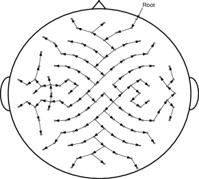
Figure 1: A graphical representation of the coding tree used in our experiments with EEG files from databases DB2a and DB2b (see Section IV).

III-A Definition of channel description order for known electrode positions

To define a channel description order we consider a tree, $T$, whose set of vertices is the set of channels, $\{1,\ldots,m\}$. We refer to $T$ as a coding tree. Specifically, in the context in which the electrode positions are known, we let $T$ be a minimum spanning tree [19, 20] of the complete graph whose set of vertices is $\{1,\ldots,m\}$, and each edge $(i,j)$ is weighted with the physical distance between electrodes of channels $i,j$. In other words, the sum of the distances between electrodes of channels $i$, $j$, over all edges $(i,j)$ of $T$, is minimal among all trees with vertices $\{1,\ldots,m\}$. We distinguish an arbitrary channel $r$ as the root, and we let the edges of $T$ be oriented so that there exists a (necessarily unique) directed path from $r$ to every other vertex of $T$. Since a tree has no cycles, the edges of $T$ induce a causal sequence of sample descriptions, for example, by arranging the edges of $T$, $e_{1},\ldots,e_{m-1}$, in a breadth-first traversal [21] order. An example of a coding tree used in our EEG compression experiments is shown in Figure 1. After describing a root channel sample, all other samples are described in the order in which their channel appear as the destination of an edge in the sequence $e_{1},\ldots,e_{m-1}$. Notice that since $T$ depends on the acquisition system but not on the signal samples, this description order may be determined off-line. The sample $x_{r}(n)$ is predicted based on samples of time up to $n-1$ of the channels $r$, $i$, where $(r,i)$ is the edge $e_{1}$; all other predictions, $\hat{x}_{i}(n)$, $i\neq r$, depend on the sample at time $n$ of channel $\ell$ and past samples of channels $\ell$, $i$, where $(\ell,i)$ is an edge of $T$.

for $n=1,2,\ldots$ do  Let $(r,i)$ be edge $e_{1}$ of $T$

$\hat{x}_{r}(n)=f_{r}(\mathbf{x}_{r}(n-1),\mathbf{x}_{i}(n-1))$

Encode $\epsilon_{r}(n)$

for $k=1,\ldots,m-1$ do  Let $(\ell,i)$ be edge $e_{k}$ of $T$

$\hat{x}_{i}(n)=f_{i}(\mathbf{x}_{i}(n-1),\mathbf{x}_{\ell}(n))$

Encode $\epsilon_{i}(n)$

end end

Algorithm 1 Coding algorithm with fixed coding tree. See sections III-A and III-B for notation and definitions.

7

7

7

7

7

7

7

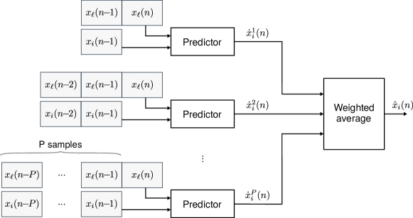
Figure 2: A representation of the weighted average predictor defined in (8), for $i\neq r$.

III-B Coding algorithm

Algorithm 1 summarizes the proposed encoding scheme. We let $\mathbf{x}_{i}(n)=x_{i}(1),\ldots,x_{i}(n)$ denote the sequence of the first $n$ samples from channel $i$, and we let $f_{i}$ be an integer valued prediction function to be defined.

We use adaptive Golomb codes [12] for the encoding of prediction errors in steps 4 and 8. Golomb codes are prefix-free codes on the integers, characterized by very simple encoding and decoding operations implemented with integer manipulations without the need for any tables; they were proven optimal for geometric distributions [22], and, in appropriate combinations, also for TSGDs [23]. A Golomb code is characterized by a positive integer parameter referred to as its order. To use Golomb codes adaptively in our application, an independent set of prediction error statistics is maintained for each channel, namely the sum of absolute prediction errors and the number of encoded samples. The statistics collected up to time $n-1$ determine the order of a Golomb code, which is combined with a Rice mapping [24] from integers to nonnegative integers to encode the prediction error at time $n$. Both statistics are halved every $F$ samples to make the order of the Golomb code more sensitive to recent error statistics and adapt quickly to changes in the prediction performance. Prediction errors are reduced modulo $|\mathcal{X}|$ and long Golomb code words are escaped so that no sample is encoded with more than a prescribed constant number of bits, $\tau$. This encoding of prediction errors is essentially the same as the one used in [25]. In particular, only Golomb code orders that are powers of two are used.

To complete the description of our encoder, we next define the prediction functions, $f_{i}$, $1\leq i\leq m$, which are used in steps 3 and 7 of Algorithm 1. For a model order $p$, we let $\mathbf{a}_{i}^{p}(n)=\{a_{i,k}(n)$, $b_{i,k}(n)\}$ denote the set of coefficient values, $a_{i,k}$, $b_{i,k}$, that, when substituted into (4), minimize the total weighted squared prediction error up to time $n$

$$E^{p}_{i}(n)=\sum_{j=1}^{n}\lambda^{n-j}\Big{(}x_{i}(j)-\hat{x}^{p}_{i}(j)\Big{)}^{2}\,,$$ (5)

where $\lambda$, $0<\lambda<1$, is an exponential decay factor parameter. This parameter has the effect of preventing $E^{p}_{i}(n)$ from growing unboundedly with $n$, and of assigning greater weight to more recent samples, which makes the prediction algorithm adapt faster to changes in signal statistics. A sequential linear predictor of order $p$ uses the coefficients $\mathbf{a}_{i}^{p}(n-1)$ to predict the sample value at time $n$ as

$$\dot{x}^{p}_{i}(n)\!=\!\sum_{k=1}^{p}\!a_{i,k}(n\!-\!1)x_{i}(n\!-\!k)+\sum_{k=0}^{p}b_{i,k}(n\!-\!1)x_{\ell}(n\!-\!k)\,,$$ (6)

and, after having observed $x_{i}(n)$, updates the set of coefficients from $\mathbf{a}_{i}^{p}(n-1)$ to $\mathbf{a}_{i}^{p}(n)$ and proceeds to the next sequential prediction. This determines a total weighted sequential absolute prediction error defined as

$$\mathcal{E}^{p}_{i}(n)=\sum_{j=1}^{n}\lambda^{n-j}\Big{|}x_{i}(j)-\dot{x}^{p}_{i}(j)\Big{|}\,.$$ (7)

Notice that each prediction $\dot{x}^{p}_{i}(j)$ in (7) is calculated with a set of model parameters, $\mathbf{a}_{i}^{p}(j-1)$, which only depends on samples that are described before $x_{i}(j)$ in Algorithm 1. These model parameters vary, in general, with $j$ (cf. (5)).

Various algorithms have been proposed to efficiently calculate $\mathbf{a}_{i}^{p}(n)$ from $\mathbf{a}_{i}^{p}(n-1)$ simultaneously for all model orders $p$, up to a predefined maximum order $P$. We resort, in particular, to a lattice algorithm (see, e.g., [16] and references therein). This calculation requires a constant number of scalar operations for fixed $P$, which is of the same order (quadratic in $P$) as the number of scalar operations that would be required by a conventional least square minimization algorithm to compute the single set of model parameters $\mathbf{a}_{i}^{P}(n)$ for the largest model order $P$. Also, we notice that using a lattice algorithm, the coefficients $\mathbf{a}_{i}^{p}(n-1)$ involved in the definition (6) of $\dot{x}^{p}_{i}(n)$ can be sequentially computed simultaneously for all $p$, $0\leq p\leq P$. Therefore, following [15], we do not fix nor estimate any specific model order but we instead average the predictions of all sequential linear predictors of order $p$, $0\leq p\leq P$, exponentially weighted by their prediction performance up to time $n-1$. Specifically, for $i\neq r$, we define

$$f_{i}(\mathbf{x}_{i}(n-1),\mathbf{x}_{\ell}(n))=\left\lfloor\frac{1}{M}\sum_{p=0}^{P}\mu_{p}(n)\dot{x}^{p}_{i}(n)\right\rceil\,,$$ (8)

where $\left\lfloor\cdot\right\rceil$ denotes rounding to the nearest integer within the quantization interval $\mathcal{X}$,

$$\mu_{p}(n)=\exp\{-\frac{1}{c}\mathcal{E}^{p}_{i}(n-1)\}\,,$$ (9)

$M$ is a normalization factor that makes $\frac{\mu_{p}(n)}{M}$ sum up to unity with $p$, $\mathcal{E}^{p}_{i}(n-1)$ is defined in (7), and $c$ is a constant that depends on $\mathcal{X}$ [15]. If the weights $\mu_{p}$ are exponential functions of the sequential squared prediction error, it is shown in [15] that the per-sample normalized squared prediction error of this predictor is asymptotically as small as the minimum normalized sequential squared prediction error among all linear predictors of order up to $P$. In our experiments, the compression ratio is systematically improved if the weights are defined instead as exponential functions of the sequential absolute prediction error as in (9). Figure 2 shows a schematic representation of the predictor $f_{i}$ defined in (8). The definition of $f_{r}$ is analogous, removing the terms corresponding to $k=0$ from (4) and (6), and letting the summation index $p$ in (8) take values in the range $1\leq p\leq P+1$.

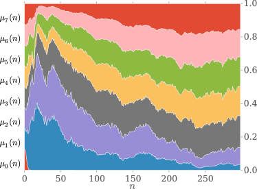
Figure 3: Stacked plot of the weights $\mu_{p}(n)$ for the first 300 samples of a 160Hz EEG channel from database DB1a.

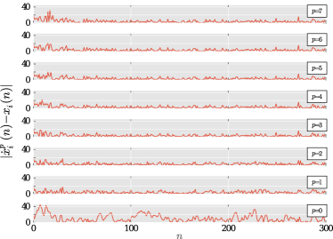
Figure 4: Absolute prediction error for the first 300 samples of the same EEG channel of Figure 3.

Figure 3 shows the evolution of the weights $\mu_{p}(n)$, $0\leq p\leq P$, during the initial segment of an EEG channel signal taken from database DB1a. Small model orders, which adapt fast, receive high weights for the very first samples. As $n$ increases, the performance of large order models improves, and these orders gain weight. Figure 4 shows the absolute prediction errors for the same EEG channel.

The overall encoding and decoding time complexity of the algorithm is linear in the number of encoded samples. Indeed, a Golomb encoding over a finite alphabet requires $O(1)$ operations and, since the set of predictions $\dot{x}^{p}_{i}(n)$, $0\leq p\leq P$, can be recursively calculated executing $O(1)$ scalar operations per sample [16], the sequential computation of $f_{i}$ requires $O(1)$ operations per sample. Regarding memory requirements, since each predictor and Golomb encoder requires a constant number of samples and statistics, the overall memory complexity of a fixed arithmetic precision implementation of the proposed encoder is $O(m)$.

III-C Definition of channel description order for unknown electrode positions

When the electrode positions are unknown, we derive the coding tree $T$ from the signal itself. To this end, we define an initial tree, $T_{0}$, with an arbitrary root channel $r$ and a set of directed edges $\{(r,i):1\leq i\leq m,i\neq r\}$ (a “star” tree). The first $B$ vector samples, $(x_{1}(n),\ldots,x_{m}(n))$, $1\leq n\leq B$, are encoded with Algorithm 1 setting $T=T_{0}$, where $B$ is a fixed block length. We update $T$ every $B$ vector samples until we reach a stoping time, $n_{s}$, to be defined. For each pair of channels $(\ell,i)$, $i\neq\ell$, $i\neq r$, we calculate the prediction $f_{i}(\mathbf{x}_{i}(n-1),\mathbf{x}_{\ell}(n))$ of $x_{i}(n)$, defined in (8), and we determine the code length, $C_{\ell,i}(n)$, of encoding the prediction error $x_{i}(n)-f_{i}(\mathbf{x}_{i}(n-1),\mathbf{x}_{\ell}(n))$ for all $n$, $1\leq n\leq n_{s}$. Notice that only the predictions $f_{i}(\mathbf{x}_{i}(n-1),\mathbf{x}_{\ell}(n))$ such that $(\ell,i)$ is an edge of $T$ are used for the actual encoding; the remaining predictions and code lengths are calculated for statistical purposes with the aim of determining a coding tree for the next block of samples.

We define a directed graph $G_{n}$ with a set of vertices $\{1,\ldots,m\}$ and a set of edges $\{(\ell,i):i\neq\ell,i\neq r\}$, where each edge $(\ell,i)$ is weighted with the average code length $\bar{C}_{\ell,i}(n)=\frac{1}{n}\sum_{i=1}^{n}C_{\ell,i}(n)$. Let $\hat{T}\left(G_{n}\right)$ be a directed tree with the same vertices as $G_{n}$, root $r$, and a subset of the edges of $G_{n}$ with minimum weight sum, i.e., $\hat{T}\left(G_{n}\right)$ is a minimum spanning tree of the directed graph $G_{n}$. Notice that, by the definition of $G_{n}$, setting $T=\hat{T}\left(G_{n}\right)$ in Algorithm 1 yields the shortest code length for the encoding of the first $n$ vector samples among all possible choices of a tree $T$ with root $r$. However, to maintain sequentiality, $T$ can only depend on samples that have already been encoded. Therefore, for each $n$ that is multiple of the block length $B$, we set $T=\hat{T}\left(G_{n}\right)$ and use this coding tree to encode the next block, $(x_{1}(i),\ldots,x_{m}(i))$, $n<i\leq n+B$. This sequential update of $T$ continues until a stopping condition is reached at some time $n_{s}$; all subsequent samples are encoded with the same tree $\hat{T}\left(G_{n_{s}}\right)$.

In our experiments, as detailed in Section IV, stopping when the compression stabilizes yields small values of $n_{s}$ and similar compression ratios as Algorithm 1 with a fixed tree as defined in Section III-A. Specifically, for the $i$-th block of samples, $i>0$, let $c_{i}$ be the sum of the edge weights of the tree $\hat{T}\left(G_{iB}\right)$, i.e., $c_{i}$ is the average code length that would be obtained for the first $iB$ vector samples with Algorithm 1 using the coding tree determined upon encoding the $i$-th block of samples. We also define $\Delta_{i}=|c_{i}-c_{i-1}|$, $i>1$, and we let $\bar{\Delta}_{i}$ be the arithmetic mean of the last $V$ values of $\Delta$, i.e., $\bar{\Delta}_{i}=V^{-1}\sum_{k=0}^{V-1}\Delta_{i-k}$, where $V$ is some small constant and $i>V$. We define $n_{s}$ as

$$n_{s}=\min\{N_{s}\}\cup\{iB:i>V,\bar{\Delta}_{i}<\gamma c_{i}\}\,,$$ (10)

where the constant $N_{s}$ establishes a maximum for $n_{s}$, and $\gamma$ is a constant.

Set $T=T_{0}$

Initialize $G_{0}$ with all edge weights equal to zero

Set $update$ = true

for $n=1,2,\ldots$ do  Encode $(x_{1}(n),\ldots,x_{m}(n))$ as in Algorithm 1

if $update$ then  Compute $G_{n}$ from $G_{n-1}$ and $C_{\ell,i}(n),i\neq\ell,i\neq r$

if $n$ is multiple of $B$ then  Set $T=\hat{T}\left(G_{n}\right)$

if Stopping condition is true then  Set $update$ = false end end end end

Algorithm 2 Coding algorithm with periodic updates of $T$. See Section III-C for notation and definitions.

6

6

6

6

6

6

The proposed encoding is presented in Algorithm 2. Step 7 of Algorithm 2 clearly requires $O(m^{2})$ operations and $O(m^{2})$ memory space. Step 9 also requires $O(m^{2})$ operations and memory space using efficient minimum spanning tree construction algorithms over directed graphs [26, 27, 28]. Thus, compared to Algorithm 1, whose time and space complexity depend linearly on $m$, steps! 7-12 of Algorithm 2 require an additional number of operations and memory space that are quadratic in $m$. These steps, however, are only executed until the stopping condition is true, which in practice is usually a relatively small number of operations (see Section IV).

III-D Near-lossless encoding

In a near-lossless setting, steps 4 and 8 of Algorithm 1 encode a quantized version, $\tilde{\epsilon}_{i}(n)$, of each prediction error, $\epsilon_{i}(n)$, defined as

$$\tilde{\epsilon}_{i}(n)=\mbox{sign}(\epsilon_{i}(n))\left\lfloor\frac{|\epsilon_{i}(n)|+\delta}{2\delta+1}\right\rfloor\,,$$ (11)

where $\lfloor z\rfloor$ denotes the largest integer not exceeding $z$. This quantization guarantees that the reconstructed value, $\tilde{x}_{i}(n)\triangleq\hat{x}_{i}(n)+\tilde{\epsilon}_{i}(n)(2\delta+1)$, differs by up to $\delta$ from $x_{i}(n)$. All model parameters and predictions are calculated with $\tilde{x}_{i}(n)$ in lieu of $x_{i}(n)$, on both the encoder and the decoder side. Thus, the encoder and the decoder calculate exactly the same prediction for each sample, and the distortion originated by the quantization of prediction errors remains bounded in magnitude by $\delta$ (in particular, it does not accumulate over time). The code lengths $C_{\ell,i}(n)$ in Algorithm 2 are also calculated for quantized versions of the prediction errors.

IV Experiments, results and discussion

IV-A Datasets

We evaluate our algorithms by running lossless ($\delta=0$) and near-lossless ($\delta>0$) compression experiments over the files of several publicly available databases, described below. In the desciption, bps stands for “bits per scalar sample”.

• DB1a and DB1b [29, 30] (BCI2000 instrumentation system): 64-channel, 160Hz, 12bps EEG of 109 subjects using the BCI2000 system. The database consists of 1308 2-minute recordings of subjects performing a motor imagery task (DB1a), and 218 1-minute calibration recordings (DB1b).

• DB2a and DB2b [31] (BCI Competition III, data set IV): 118-channel, 1000Hz, 16bps EEG of 5 subjects performing motor imagery tasks (DB2a). The average duration over the 8 recordings of the database is 39 minutes, with a minimum of almost 13 minutes and a maximum of almost 50 minutes. DB2b is a 100Hz downsampled version of DB2a.

• DB3 [32] (BCI Competition IV): 59-channel, 1000Hz, 16bps EEG of 7 subjects performing motor imagery tasks. The database is comprised of 14 recordings of lengths ranging from 29 to 41 minutes, with an average duration of 35 minutes.

• DB4 [33]: 31-channel, 1000Hz, 16bps EEG of 15 subjects performing image classification and recognition tasks. The database consists of 373 recordings with an average duration of 3.5 minutes, a minimum of 3.3 minutes, and a maximum of 5.5 minutes.

• DB5 [29, 34] (Physikalisch-Technische Bundesanstalt (PTB) Diagnostic ECG Database): standard 12-lead, 1000Hz, 16bps ECG. This database consists of 549 recordings taken from 290 subjects, with an average duration of 1.8 minutes, a minimum of 0.5 minutes and a maximum of 2 minutes.

For the ECG data we extracted leads $i$, $ii$, $v_{1}\ldots v_{6}$, to form an 8-channel signal from the standard 12-lead ECG records [18] (the remaining 4 leads are linear combinations of these 8 channels). Each of these ECG leads is a linear combination of electrode measures, which represent heart depolarization along the direction of a certain vector; the notion of distance between channels that we use to determine a coding tree for Algorithm 1 in this case is the angle between these vectors (see Section III-A).

IV-B Evaluation procedure

For each database, we compress each data file separately, and we calculate the compression ratio (CR), in bits per sample, defined as $\text{CR}=L/N$, where $N$ is the sum of the number of scalar samples over all files of the database, and $L$ is the sum of the number of bits over all compressed files of the database. Notice that smaller values of CR correspond to better compression performance. The above procedure is repeated for $\delta=0,1,2,\ldots,10$. Each discrete sample reconstructed by the decoder differs by no more than $\delta$ from its original value, which translates to a maximum difference between signal samples measured in microvolts ($\mu V$) that depends on the resolution of the acquisition system. The scaling factor that maps discrete sample differences to voltage differences in $\mu V$ is 1 for DB1a and DB1b, 0.1 for DB2a, DB2b and DB3, approximately 0.84 for DB4, and 0.5 for DB5.

In the experiments, we set the maximum prediction order in (8) to $P=7$, the exponential decay factor in (5) to $\lambda=0.99$, and the constant $c$ in (9) to a baseline value $c=32$ (in fact, to improve numerical stability in (8), we found it useful to increment [decrement] $c$ whenever the normalization factor $M$ falls below [above] a certain threshold). For Golomb codes, we set the upper bound on code word length, $\tau$, to 4 times the number of bits per sample of the original signal, and the interval between halvings of statistics to $F=16$. For each database, we executed algorithm 1 with $\delta=0$ and all possible choices of a root channel $r$ of the coding tree; the difference between the best and worst root choices was always less than $0.01$bps. All the results reported in the sequel were obtained, for each database, with the root channel that yielded the median compression ratio for that database.

TABLE II: Compression ratio of Algorithm 1 and best compression ratio in [7, 8, 10] (in parenthesis).

$\delta$	DB1a	DB1b	DB2a	DB2b	DB3	DB4	DB5
0	(5.37) 4.70	(5.45) 4.79	(5.69) 5.21	(7.90) 6.93	(6.46) 5.42	(3.73) 3.58	(5.03) 4.78
5	1.97	(2.51) 1.98	2.34	(4.76) 3.54	(7.05) 2.43	1.79	1.99
10	1.55	(1.81) 1.55	1.84	(3.85) 2.73	(6.08) 1.88	1.53	1.59

TABLE III: Compression ratio of Algorithm 2 and percentage relative difference with respect to Algorithm 1 (in parenthesis).

$\delta$	DB1a	DB1b	DB2a	DB2b	DB3	DB4	DB5
0	(3.40) 4.54	(3.55) 4.62	(1.15) 5.15	(2.02) 6.79	(0.55) 5.39	(-0.56) 3.60	(-0.21) 4.79
5	(3.05) 1.91	(3.54) 1.91	(2.14) 2.29	(3.95) 3.40	(1.23) 2.40	(-0.56) 1.80	(-1.01) 2.01
10	(1.94) 1.52	(1.94) 1.52	(1.09) 1.82	(4.40) 2.61	(0.53) 1.87	(-0.65) 1.54	(-1.26) 1.61

IV-C Compression Results for Algorithm 1

The compression ratio obtained with Algorithm 1 for each database, as a function of $\delta$, is shown in Table II and plotted in Figure 5. For $\delta=0$ (i.e., lossless compression), Table II also shows, in parenthesis, the compression ratio obtained with the reference software implementation of ALS, configured for compression rate optimization. For $\delta>0$, the value in parenthesis is the best compression reported in [7, 8], where several compression algorithms are tested with EEG data taken from databases DB1a, DB2b, and DB3. As Table II shows, the compression ratios obtained with Algorithm 1 are the best in all cases. In the near-lossless mode with $\delta>0$, the algorithm is designed to guarantee a worst-case error magnitude of $\delta$ in the reconstruction of each sample. For completeness, it may also be of interest to assess the performance of the algorithm under other disortion measures (e.g. mean absolute error, or SNR), for which it was not originally optimized. Such an assessment is presented in the Appendix.

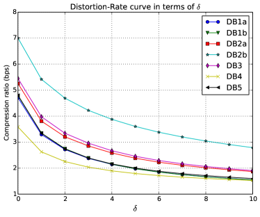
Figure 5: Compression ratio obtained with Algorithm 1 for each value of $\delta$ and all databases. The plots of DB1a, DB1b, and DB5 overlap.

IV-D Compression Results for Algorithm 2

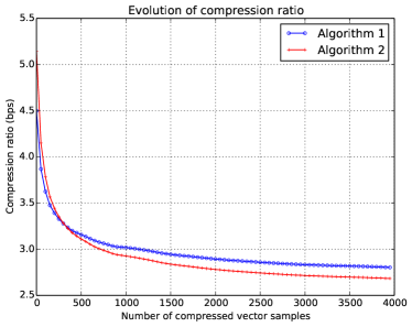
Figure 6: Evolution in time of the average compression ratio obtained with Algorithm 1 and Algorithm 2 for DB2b with $\delta=10$.

For Algorithm 2, we set the block size $B$ equal to $50$, and for the stopping condition in the coding tree $T$ learning stage, we set $V=5$, $\gamma=0.03$, and $N_{s}=3000$ (see Section III-C). The compression ratio obtained with Algorithm 2, for each database and for different values of $\delta$, is shown in Table III. The table also shows, in parenthesis, the percentage relative difference, $\frac{CR_{1}-CR_{2}}{CR_{1}}\times 100$, between the compression ratios $CR_{1}$ and $CR_{2}$ obtained with Algorithm 1 and Algorithm 2, respectively, with respect to $CR_{1}$.

We observe that both algorithms achieve very similar compression ratios in all cases. In fact, for all the databases except DB4 and DB5, Algorithm 2 yields better results. Thus, in most of the tested cases, we obtain better compression ratios by constructing a coding tree from learned compression statistics rather than based on the fixed geometry, and this compression ratio improvement is sufficiently large to overcome the cost incurred during the training segment of the signal, when a good coding tree is not yet known. This is graphically illustrated in Figure 6; for each $n$, in steps of 50 up to a maximum of 4,000 vector samples, the figure plots the compression ratio obtained up to the encoding of vector sample $n$, averaged over all files of the database DB2b with $\delta=10$. For databases DB4 and DB5, although Algorithm 2 does not surpass Algorithm 1, the results are extremely close.

Ultimately, which of the algorithms will perform better is a function of the accuracy of the hypothesis that closer physical proximity of electrodes implies higher correlation (surely other physical factors must also affect correlation), and of the heuristic employed to determine a stopping time for the learning stage of Algorithm 2. The longer we let the algorithm learn, the higher the likelihood that it will converge to the best coding tree (which may or may not coincide with the tree of Algorithm 1), but the higher the computational cost. The results in Table III suggest that the physical distance hypothesis seems to be more accurate for DB4 and DB5 than for the other databases, and that the heuristic for $n_{s}$ chosen in the experiments offers a good compromise of computational complexity against compression performance.

IV-E Computational complexity

As mentioned, deriving a coding tree from the signal data in Algorithm 2 comes at the price of additional memory requirements and execution time compared to Algorithm 1. These additional resources are required while the algorithm is learning a coding tree $T$. The stopping time, $n_{s}$, of this learning stage, is determined adaptively, as specified in (10). Table IV shows the mean and standard deviation of $n_{s}$, taken over the files of each database. We notice that, in general, the update of $T$ is stopped after a few thousand vector samples. The percentage fraction of the mean stopping time with respect to the mean total number of vector samples in each database is also shown, in parenthesis, in Table IV. We observe that $n_{s}$ is less than 1% of the number of vector samples in most cases and it is never more than 10% of that number.

TABLE IV: Mean and standard deviation of the stopping time, $n_{s}$, obtained for each file on different databases. The percentage fraction of the mean stopping time with respect to the mean total number of vector samples in each database is shown in parenthesis.

$\delta$	DB1a	DB1b	DB2a	DB2b	DB3	DB4	DB5
0	(3.49) 637 $\pm$ 154	(6.78) 662 $\pm$ 210	(0.04) 875 $\pm$ 144	(0.3) 713 $\pm$ 222	(0.06) 743 $\pm$ 176	(0.58) 1227 $\pm$ 346	(1.40) 1523 $\pm$ 398
5	(4.10) 747 $\pm$ 189	(7.81) 762 $\pm$ 244	(0.04) 1050 $\pm$ 229	(0.44) 1038 $\pm$ 400	(0.09) 1046 $\pm$ 311	(0.58) 1242 $\pm$ 348	(1.76) 1911 $\pm$ 507
10	(3.79) 690 $\pm$ 180	(7.35) 717 $\pm$ 236	(0.04) 1044 $\pm$ 220	(0.46) 1081 $\pm$ 439	(0.09) 1075 $\pm$ 339	(0.55) 1172 $\pm$ 327	(1.60) 1735 $\pm$ 439

We measured the total time required to compress and decompress all the files in all the testing databases. Algorithm 1 was implemented in the C language, and Algorithm 2 in C++. They were compiled with GCC 4.8.4, and run with no multitasking (single thread), on a personal computer with a 3.4GHz Intel i7 4th generation processor, 16GB of RAM, and under a Linux 3.16 kernel. Table V shows the average time required by our implementation of Algorithm 2 to compress and decompress a vector sample for each database. The results are given for the overall processing of files and for each main stage of the algorithm separately, namely the first stage during which the coding tree $T$ is being updated and the second stage during which $T$ is fixed.

Notice that for a fixed coding tree, the execution time is linear in the number of scalar samples, with a very small variation from dataset to dataset. The results that we obtained for Algorithm 1 are similar (smaller in all cases) to those reported for the second stage of Algorithm 2. On the other hand, for vector samples taken before the stoping time $n_{s}$, the average compression and decompression time is approximately proportional to $m^{2}$, as expected. For most databases, this compression time rate exceeds the sampling rate and, thus, real time compression and decompression would require buffering data to compensate for this rate difference; notice that the size required for such a buffer can be estimated from the upper bound $N_{s}$ on $n_{s}$, and the average compression time for each stage of the algorithm. In general, with the exception of DB1a and DB1b that are comprised of short files with a large number of channels, the impact of the additional computational cost for learning the coding tree is relatively small in relation to the overall processing time.

TABLE V: Average processing time (in microseconds) of a vector sample for Algorithm 2. Time averages are given for the overall processing of files and also discriminating the period of time during which the coding tree is being updated ($n\leq n_{s}$) from the period of time in which it is fixed ($n>n_{s}$).

		DB1a	DB1b	DB2a	DB2b	DB3	DB4	DB5
$m$		64	64	118	118	59	31	8
$n>n_{s}$	coding	63.3	63.3	118.4	119.4	58.6	30.4	7.2
$n>n_{s}$	decoding	63.6	63.6	118.8	119.2	58.9	30.4	7.6
$n\leq n_{s}$	coding	7661.4	7667.1	26799.3	27190.6	6304.7	1202.9	65.9
$n\leq n_{s}$	decoding	7887.5	7889.2	27811.6	28367.1	6516.0	1223.2	66.7
Global	coding	320.7	562.0	130.5	217.6	60.8	37.2	8.1
Global	decoding	328.7	576.7	131.3	221.6	61.2	37.4	8.5

Algorithm 1 has also been ported to a low power MSP432 microcontroller running at 48MHz, where it requires an average of $3.21$ milliseconds to process a single scalar sample, allowing a maximum real-time processing of 16 channels at 321Hz. In order to fit within the memory of the MSP432, the maximum order of the predictors was set to $P=4$, resulting in a slight performance degradation with respect to that reported in Table II. The resulting memory footprint is $42.5$kB of flash memory, and $26.7$kB of RAM. Further details and advances in this direction will be published elsewhere.

V Conclusions

The space and time redundancy in both EEG and ECG can be effectively reduced with a predictive adaptive coding scheme in which each channel is predicted through an adaptive linear combination of past samples from the same channel, together with past and present samples from a designated reference channel. Selecting this reference channel according to the physical distance between the sensors that register the signals is a very simple approach, which yields good compression rates and, since it can be implemented off-line, incurs no additional computational effort at coding or decoding time. When sensor positions are not known a priori, we propose a scheme for inter-channel redundancy analysis based on efficient minimum spanning tree construction algorithms for directed graphs. Both proposed encoding algorithms are sequential, and thus suitable for low-latency applications. In addition, the number of operations per time sample, and the memory requirements depend solely on the number of channels of the acquisition system, which makes the proposed algorithms attractive for hardware implementations. This is especially true for Algorithm 1, whose memory and time requirements depend linearly on the number of channels. In the case of Algorithm 2 these requirements are quadratic in the number of channels during the learning stage, which might make a pure hardware implementation more difficult if this number is large.

[Other distortion measures]

TABLE VI: MAE (in $\mu V$) obtained with Algorithm 1 and Algorithm 2 (in parenthesis) for different values of $\delta$.

$\delta$	DB1a	DB1b	DB2a	DB2b	DB3	DB4	DB5
5	( 2.69) 2.69	( 2.70) 2.70	( 0.27) 0.27	( 0.27) 0.27	( 0.27) 0.27	( 2.30) 2.29	( 1.36) 1.36
10	( 5.00) 5.00	( 5.08) 5.09	( 0.52) 0.52	( 0.52) 0.52	( 0.52) 0.52	( 4.39) 4.38	( 2.59) 2.58

TABLE VII: SNR (in dB) obtained with Algorithm 1 and Algorithm 2 (in parenthesis) for different values of $\delta$.

$\delta$	DB1a	DB1b	DB2a	DB2b	DB3	DB4	DB5
5	(27.79) 27.59	(27.40) 26.98	(49.47) 49.47	(49.48) 49.47	(48.11) 48.11	(59.70) 59.69	(53.07) 52.89
10	(22.35) 22.16	(21.87) 21.46	(43.83) 43.83	(43.84) 43.83	(42.52) 42.52	(54.07) 54.09	(47.48) 47.33

TABLE VIII: SNR (in dB) obtained with Algorithm 1 using a value of $\delta$ that corresponds approximately to 1 $\mu V$ for each database. The specific value of $\delta$ used in each case is shown in parenthesis.

DB1a	DB1b	DB2a	DB2b	DB3	DB4	DB5
(1) 39.26	(1) 38.69	(10) 43.83	(10) 43.83	(10) 42.52	(1) 71.46	(2) 59.87

For the cases where $\delta>0$ (near-lossless) we compute the mean absolute error (MAE), and the signal to noise ratio (SNR) given respectively by

$$\mathrm{MAE} =\frac{1}{Nm}\sum_{i=1}^{m}\sum_{n=1}^{N}|x_{i}(n)-\tilde{x}_{i}(n)|\,,$$

$$\mathrm{SNR} =10\log_{10}\frac{\sum_{i=1}^{m}\sum_{n=1}^{N}x_{i}(n)^{2}}{\sum_{i=1}^{m}\sum_{n=1}^{N}(x_{i}(n)-\tilde{x}_{i}(n))^{2}}\,.$$

Figures 7 and 8 show plots of the MAE and the SNR, respectively, against the compression ratio obtained with Algorithm 1 for different values of $\delta$. The plots for Algorithm 2 are very similar and thus omitted. The MAE and SNR obtained with both algorithms for $\delta=5$ and $\delta=10$ are shown in Tables VI and VII, respectively. We observe that, in every case, the MAE is close to one half of the maximum allowed distortion given by $\delta$ (appropriately scaled to $\mu V$). This matches well the behavior expected from a TSGD hypothesis on the prediction errors. The SNR varies significantly among databases for a fixed value of $\delta$, due to both the difference in scale and the difference in power (in $\mu V^{2}$) among the databases. Table VIII shows the SNR obtained using a value of $\delta$ that corresponds approximately to 1 $\mu V$ for each database. We still observe very different values of SNR, which is explained by the difference in power of the signals. We verified by direct observation that, as expected by design, the maximum absolute error (M*AE) for Algorithm 1 is equal to $\delta$ in every case.

Table IX compares the SNR and M*AE of Algorithm 1 with the results published in [8]. For the comparison, we selected the value of $\delta$ that yields the compression ratio closest to that reported in [8] in each case. We observe that the SNR is in general better for the best algorithm in [8], except in the case of DB3, where Algorithm 1 attains similar (or better) compression ratios with lossless compression (infinite SNR). The M*AE is much smaller for Algorithm 1 in all cases. These results should be taken with a grain of salt, though, given that our scheme, contrary to that of [8], does not target SNR.

TABLE IX: Best compression ratio / distortion reported in [8] (in parenthesis), and distortion obtained with Algorithm 1 for the choice of $\delta$ that yields the closest compression ratio.

Database	CR (bps)	SNR (db)	M*AE ($\mu V$)
DB1b	(3.32) 3.35	(47.3) 38.7	(2.85) 1
DB1b	(2.42) 2.39	(36.1) 30.9	(5.35) 3
DB2b	(5.26) 5.35	(80.0) 60.8	(0.73) 0.1
DB2b	(4.29) 4.15	(73.9) 53.5	(1.22) 0.3
DB3	(6.27) 5.42	(80.0) $\mathbf{\infty}$	(0.67) 0
DB3	(5.33) 5.42	(66.0) $\mathbf{\infty}$	(1.19) 0

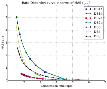
Figure 7: Rate-Distortion curve in terms of MAE obtained with Algorithm 1 when $\delta$ takes the values $0,1,\ldots,10$ for all databases.

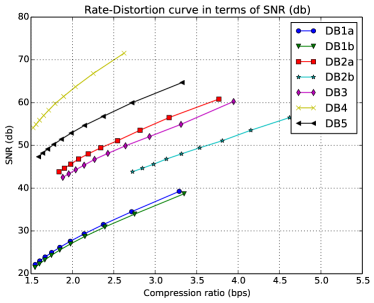
Figure 8: Rate-Distortion curve in terms of SNR obtained with Algorithm 1 when $\delta$ takes the values $1,2,\ldots,10$ for all databases.

We also analyze the variation of the MAE and SNR over the channels for all the databases and its dependence on $\delta$. Figures 9(a)-(c) show the MAE and SNR against the compression ratio for all channels with $\delta=\{1,5,10\}$ for the database DB1a. All channels have a similar behavior for the MAE and SNR, with lower dispersion for the MAE than the SNR. Since the mean square error has a dispersion similar to the MAE (not shown), the greater dispersion of the SNR is explained by the variation of the power among channels. This dispersion can be reduced by selecting a specific value of $\delta$ for each channel, depending on the power of its signal. The behavior for MAE and SNR is similar in all the databases, and, thus, it is reported only for DB1a for succinctness.

Figures 10 and 11 summarize the mean and standard deviation of both the MAE and the SNR measures over all channels, for each database for different values of $\delta$. One standard deviation is shown as an errorbar with the mean for each $\delta$. Again, a similar behavior among all the databases is observed, with lower dispersion in the MAE, increasing with $\delta$ and almost constant dispersion for the SNR.

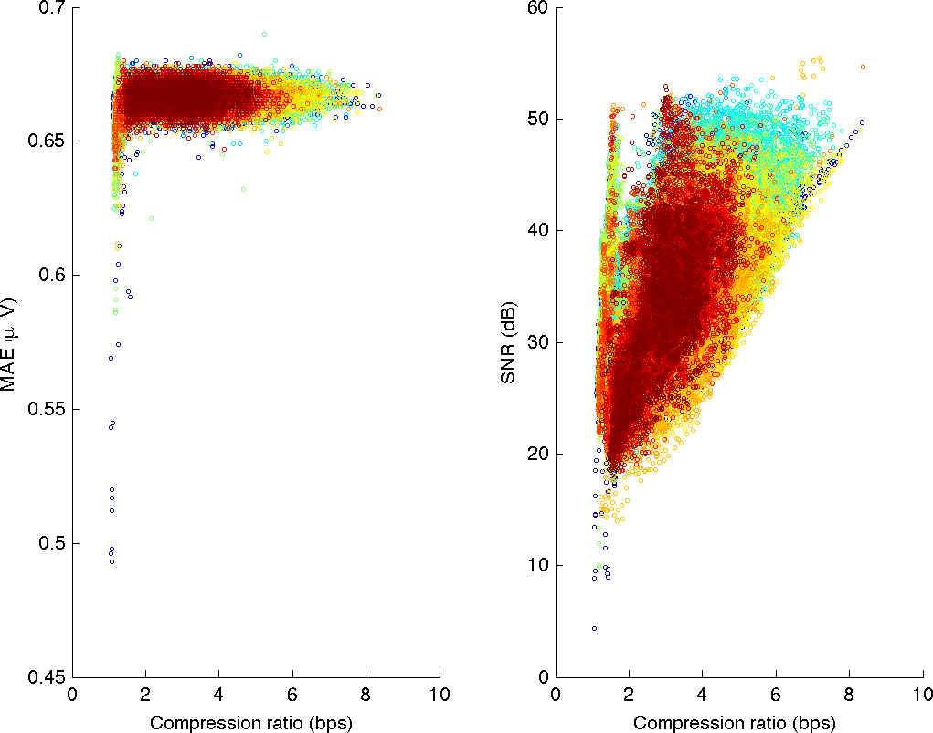
(a)

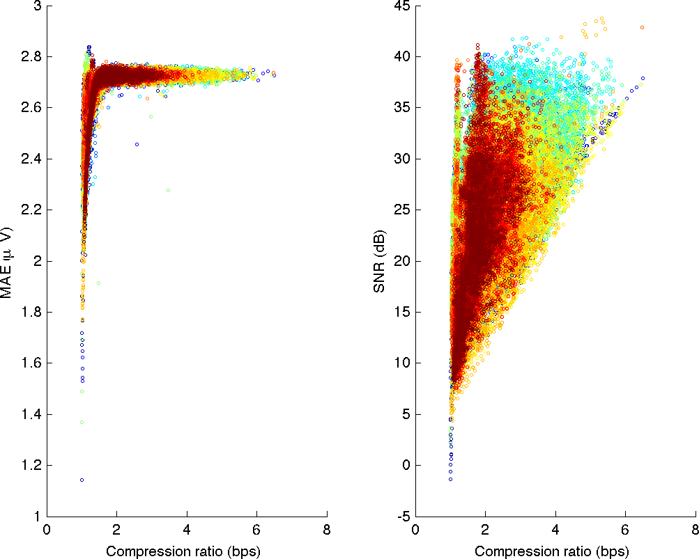
(b)

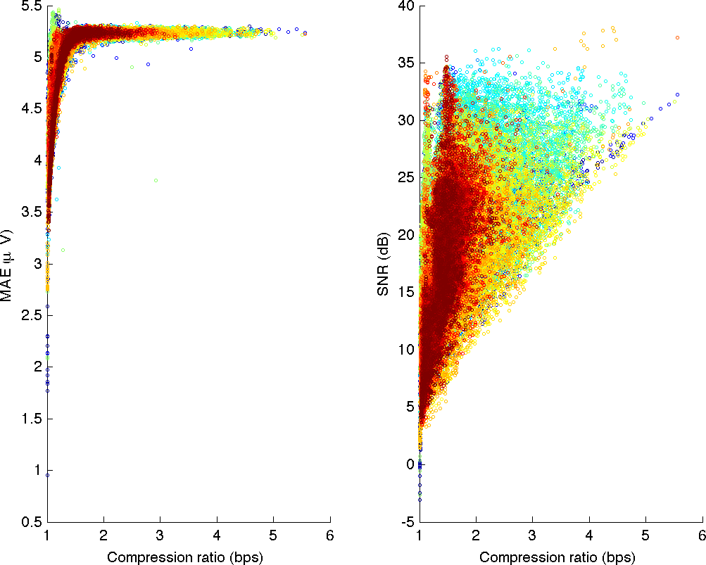
(c)

Figure 9: (a)–(c) Rate-Distortion values for all channels and files in terms of MAE and SNR obtained with Algorithm 1 when $\delta$ takes the values (a) $1$, (b) $5$ and (c) $10$ for database DB1a. Each channel is plotted with a different color.

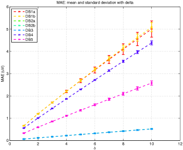
Figure 10: MAE mean over all channels and its standard deviation as an errorbar when $\delta$ takes the values $1,2,\dots,10$ for all databases.

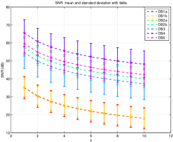
Figure 11: SNR mean over all channels and its standard deviation as an errorbar when $\delta$ takes the values $1,2,\dots,10$ for all databases.

References

- [1] A. Koski, “Lossless ECG encoding,” Computer Methods and Programs in Biomedicine, vol. 52, no. 1, pp. 23 – 33, 1997.
- [2] G. Antoniol and P. Tonella, “EEG data compression techniques,” IEEE Trans. Biomedical Engineering, vol. 44, no. 2, pp. 105–114, Feb 1997.
- [3] Z. Arnavut and H. Koak, “Lossless EEG signal compression,” in Proc. 5th Int. Conf. Soft Computing, Computing with Words and Perceptions in System Analysis, Decision and Control, Sept 2009.
- [4] K. Srinivasan, J. Dauwels, and M. R. Reddy, “A two-dimensional approach for lossless EEG compression,” Biomedical Signal Processing and Control, vol. 6, no. 4, pp. 387 – 394, 2011.
- [5] N. Memon, X. Kong, and J. Cinkler, “Context-based lossless and near-lossless compression of EEG signals,” IEEE Trans. Inform. Technology in Biomedicine, vol. 3, no. 3, pp. 231–238, Sept 1999.
- [6] Y. Wongsawat, S. Oraintara, T. Tanaka, and K. Rao, “Lossless multi-channel EEG compression,” in Proc. 2006 IEEE Int. Symp. Circuits and Systems, May 2006.
- [7] K. Srinivasan, J. Dauwels, and M. Reddy, “Multichannel EEG compression: Wavelet-based image and volumetric coding approach,” IEEE Journal of Biomedical and Health Informatics, vol. 17, no. 1, pp. 113–120, Jan 2013.
- [8] J. Dauwels, K. Srinivasan, M. Reddy, and A. Cichocki, “Near-lossless multichannel EEG compression based on matrix and tensor decompositions,” IEEE Journal of Biomedical and Health Informatics, vol. 17, no. 3, pp. 708–714, May 2013.
- [9] Q. Liu, M. Sun, and R. Sclabassi, “Decorrelation of multichannel EEG based on Hjorth filter and graph theory,” in Proc. 6th Int. Conf. Signal Proc., vol. 2, Aug 2002, pp. 1516–1519 vol.2.
- [10] ISO/IEC 14496-3:2005/Amd.2:2006, Information technology—Coding of audio-visual objects—Part 3: Audio, 3rd Ed. Amendment 2: Audio Lossless Coding (ALS), new audio profiles and BSAC extensions.
- [11] Y. Kamamoto, N. Harada, and T. Moriya, “Interchannel dependency analysis of biomedical signals for efficient lossless compression by MPEG-4 ALS,” in Acoustics, Speech and Signal Processing, 2008. ICASSP 2008. IEEE International Conference on, March 2008, pp. 569–572.
- [12] S. W. Golomb, “Run-length encodings,” IEEE Trans. Inform. Theory, vol. 12, pp. 399–401, Jul. 1966.
- [13] N. Merhav, G. Seroussi, and M. Weinberger, “Coding of sources with two-sided geometric distributions and unknown parameters,” IEEE Trans. Inform. Theory, vol. 46, no. 1, pp. 229–236, Jan 2000.
- [14] J. Rissanen, “Universal coding, information, prediction, and estimation,” IEEE Trans. Inform. Theory, vol. 30, pp. 629–636, Jul. 1984.
- [15] A. Singer and M. Feder, “Universal linear prediction by model order weighting,” IEEE Trans. Sig. Processing, vol. 47, no. 10, pp. 2685–2699, Oct 1999.
- [16] G.-O. Glentis and N. Kalouptsidis, “A highly modular adaptive lattice algorithm for multichannel least squares filtering,” Signal Processing, vol. 46, no. 1, pp. 47–55, Sep. 1995.
- [17] C. on methods of clinical examination in electroencephalography, “Report of the committee on methods of clinical examination in electroencephalography,” Electroencephalography and Clinical Neurophysiology, vol. 10, no. 2, pp. 370 – 375, 1958.
- [18] P. Macfarlane, A. van Oosterom, O. Pahlm, P. Kligfield, M. Janse, and J. Camm, Eds., Comprehensive Electrocardiology, 2nd ed. London: Springer, 2010, vol. 1.
- [19] O. Borůvka, “O jistém problému minimálním,” Práce mor. přírodověd. spol. v Brně, vol. 3, pp. 37––58, 1926.
- [20] J. B. Kruskal, “On the shortest spanning subtree of a graph and the traveling salesman problem,” in Proceedings of the American Mathematical Society, 7, 1956.
- [21] E. F. Moore, “The shortest path through a maze,” in Proceedings of the International Symposium on the Theory of Switching. Harvard University Press, 1959, pp. 285–292.
- [22] R. G. Gallager and D. C. Van Voorhis, “Optimal source codes for geometrically distributed integer alphabets,” IEEE Trans. Inform. Theory, vol. 21, pp. 228–230, mar 1975.
- [23] N. Merhav, G. Seroussi, and M. J. Weinberger, “Optimal prefix codes for two-sided geometric distributions,” IEEE Trans. Inform. Theory, vol. IT-46, pp. 121–135, Jan. 2000.
- [24] R. F. Rice, “Some practical universal noiseless coding techniques — Parts I–III,” jet Propulsion Lab., Pasadena, CA, Tech. Reps. JPL-79-22, JPL-83-17, and JPL-91-3, Mar. 1979, Mar. 1983, Nov. 1991.
- [25] M. Weinberger, G. Seroussi, and G. Sapiro, “The LOCO-I lossless image compression algorithm: principles and standardization into JPEG-LS,” IEEE Trans. Image Processing, vol. 9, no. 8, pp. 1309–1324, Aug 2000.
- [26] R. E. Tarjan, “Finding optimum branchings,” Networks, vol. 7, no. 1, pp. 25–35, 1977.
- [27] P. M. Camerini, L. Fratta, and F. Maffioli, “A note on finding optimum branchings.” Networks, vol. 9, no. 4, pp. 309–312, 1979.
- [28] H. Gabow, Z. Galil, T. Spencer, and R. Tarjan, “Efficient algorithms for finding minimum spanning trees in undirected and directed graphs,” Combinatorica, vol. 6, no. 2, pp. 109–122, 1986.
- [29] A. L. Goldberger, L. A. N. Amaral, L. Glass, J. M. Hausdorff, P. C. Ivanov, R. G. Mark, J. E. Mietus, G. B. Moody, C.-K. Peng, and H. E. Stanley, “PhysioBank, PhysioToolkit, and PhysioNet: Components of a new research resource for complex physiologic signals,” Circulation, vol. 101, no. 23, 2000 (June 13).
- [30] G. Schalk, D. McFarland, T. Hinterberger, N. Birbaumer, and J. Wolpaw, “BCI2000: a general-purpose brain-computer interface (BCI) system,” IEEE Trans. Biomedical Engineering, vol. 51, no. 6, pp. 1034–1043, June 2004.
- [31] G. Dornhege, B. Blankertz, G. Curio, and K. Muller, “Boosting bit rates in noninvasive EEG single-trial classifications by feature combination and multiclass paradigms,” IEEE Trans. Biomedical Engineering, vol. 51, no. 6, pp. 993–1002, June 2004.
- [32] B. Blankertz, G. Dornhege, M. Krauledat, K.-R. Müller, and G. Curio, “The non-invasive Berlin brain–computer interface: Fast acquisition of effective performance in untrained subjects,” NeuroImage, vol. 37, no. 2, pp. 539 – 550, 2007.
- [33] A. Delorme, G. A. Rousselet, M. J.-M. Macé, and M. Fabre-Thorpe, “Interaction of top-down and bottom-up processing in the fast visual analysis of natural scenes,” Cognitive Brain Research, vol. 19, no. 2, pp. 103 – 113, 2004.
- [34] R. Bousseljot, D. Kreiseler, and A. Schnabel, “Nutzung der EKG-Signaldatenbank CARDIODAT der PTB über das Internet,” Biomedizinische Technik, vol. 40, no. 1, pp. S317–S318, 1995.