Pinning down neutrino oscillation parameters in the 2–3 sector with a mgnetised atmospheric neutrino detector: a new study

Abstract

We determine the sensitivity to neutrino oscillation parameters from a study of atmospheric neutrinos in a magnetised detector such as the ICAL at the proposed India-based Neutrino Observatory. In such a detector that can separately count $\nu_{\mu}$ and $\overline{\nu}_{\mu}$-induced events, the relatively smaller (about 5%) uncertainties on the neutrino–anti-neutrino flux ratios translate to a constraint in the $\chi^{2}$ analysis that results in a significant improvement in the precision with which neutrino oscillation parameters such as $\sin^{2}\theta_{23}$ can be determined. Such an effect is unique to all magnetisable detectors and constitutes a great advantage in determining neutrino oscillation parameters using such detectors. Such a study has been performed for the first time here. Along with an increase in the kinematic range compared to earlier analyses, this results in sensitivities to oscillation parameters in the 2–3 sector that are comparable to or better than those from accelerator experiments where the fluxes are significantly higher. For example, the $1\sigma$ precisions on $\sin^{2}\theta_{23}$ and $|\Delta{m^{2}_{32(31)}}|$ achievable for 500 kTon yr exposure of ICAL are $\sim 9\%$ and $\sim 2.5\%$ respectively for both normal and inverted hierarchies. The mass hierarchy sensitivity achievable with this combination when the true hierarchy is normal (inverted) for the same exposure is $\Delta\chi^{2}\approx 8.5$ ($\Delta\chi^{2}\approx 9.5$).

1 Introduction

One of the open questions in neutrino physics is the mass ordering of the neutrinos; whether they are ordered normally or inverted. Many experiments intend to determine the mass ordering, of which the 50 kton Iron Calorimeter (ICAL) detector at the proposed India-based Neutrino observatory is one ambitious experiment [1]. ICAL will be a magnetised iron calorimeter mainly sensitive to muons produced in the charged-current (CC) interactions of atmospheric muon neutrinos (and anti-neutrinos) with the iron target in the detector. It can distinguish CC muon-neutrino-induced events from anti-neutrino-induced ones since the former interaction produces $\mu^{-}$ while the latter produces $\mu^{+}$ in the detector and ICAL has excellent muon charge identification (cid) capability. This is also crucial to determine precisely the momentum of the muons through bending in the magnetic field. Since matter effects are different between neutrino and anti-neutrino propagation in the Earth, this feature can help resolve the neutrino mass ordering by determining the sign of the 2–3 mass-squared difference $\Delta m^{2}_{32}\equiv m^{2}_{3}-m^{2}_{2}$, $m_{i},~{}i=1,2,3$, being the neutrino mass eigenstates [2]. In addition, the matter effects improve the sensitivity to the magnitude $|\Delta m^{2}_{32}|$ of this mass-squared difference as well as to the 2–3 mixing angle, $\theta_{23}$, provided the across-generation mixing angle $\theta_{13}$ is rather well-known, which is indeed the case [3, 4, 5, 6, 7].

Many previous analyses have been reported, projecting the sensitivities of ICAL detector to oscillation parameters in the 2–3 sector [8, 9, 10, 1] as also the mass ordering. The sensitivity to mass hierarchy is directly proportional to the value of $\theta_{13}$ which is quite precisely known [11, 12, 13, 14, 15, 16]. It also depends on the ability of ICAL to separate neutrino and anti-neutrino events which is possible since ICAL is magnetised. While there is an uncertainty of about 20% on the atmospheric neutrino fluxes themselves, the uncertainty on their ratios is much smaller, about 5%, and was ignored in earlier analyses [8, 9, 10]. In this paper, we show that this smaller uncertainty on the ratio acts as a constraint that in turn significantly shrinks the allowed parameter space, especially for $\sin^{2}\theta_{23}$. For instance, we will see that the precision on $\sin^{2}\theta_{23}$ decreases from 13% to 9% in a certain analysis mode when this constraint is included. This is generally true for all magnetised detectors. To our knowledge such an effect has not been discussed in the literature earlier.

The paper is structured as follows. All the results in this paper are with detailed simulation studies of the physics processes at the ICAL detector. The main steps involved in this are neutrino event generation, inclusion of detector responses and efficiencies, inclusion of oscillations, binning in observables and $\chi^{2}$ analysis. The procedure of neutrino event generation with the NUANCE neutrino [17] generator and the implementation of oscillations are discussed in detail in Section 2. The choice of observables and kinematic regions used in the analysis, along with the inclusion of detector responses are discussed in detail in Section 3. The effect of increasing the energy range of observed muons is also explained in this section. The detailed $\chi^{2}$ analysis and a discussion of the systematic errors that have been considered are presented in Section 4. The results of precision measurements and hierarchy sensitivity studies are shown in Section 5. The impact of the additional pull in the $\nu/\overline{\nu}$ flux ratio implemented in this analysis is discussed in detail in Section 6. The summary and conclusions are given in Section 7.

2 Neutrino events generation

The interactions of interest in ICAL are the CC interactions of $\nu_{\mu}$ and $\overline{\nu}_{\mu}$ with the iron target in ICAL. These $\nu_{\mu}$ ($\overline{\nu}_{\mu}$) in ICAL come from both $\nu_{\mu}$ and $\nu_{e}$ atmospheric fluxes via $\nu_{\mu}\rightarrow\nu_{\mu}$ and $\nu_{e}\rightarrow\nu_{\mu}$ oscillations. The first channel gives the number of $\nu_{\mu}$ events which have survived and the second, subdominant, one gives the number from oscillations of $\nu_{e}$ to $\nu_{\mu}$. The number of events ICAL sees will be a sum of these events. Thus,

$$\frac{d^{2}N}{dE_{\mu}d\cos\theta_{\mu}} = t\times{n_{d}}\times\int{dE_{\nu}d\cos\theta_{\nu}d\phi_{\nu}}\times$$ (1)

$$\hskip 14.22636pt\left[P_{\mu\mu}\frac{d^{3}\Phi_{\mu}}{dE_{\nu}d\cos\theta_{\nu}d\phi_{\nu}}+P_{e\mu}\frac{d^{3}\Phi_{e}}{dE_{\nu}d\cos\theta_{\nu}d\phi_{\nu}}\right]\times\frac{d\sigma_{\mu}(E_{\nu})}{dE_{\mu}d\cos\theta_{\mu}}~{},$$

where $n_{d}$ is the number of target nucleons in the detector, $\sigma_{\mu}$ is the differential neutrino interaction cross section in terms of the energy and direction of the CC lepton produced, $\Phi_{\mu}$ and $\Phi_{e}$ are the $\nu_{\mu}$ and $\nu_{e}$ fluxes and $P_{\alpha\beta}$ is the oscillation probability of $\nu_{\alpha}\rightarrow\nu_{\beta}$.

The number of unoscillated events over an exposure time $t$ in a bin of ($E_{\mu},\cos\theta_{\mu}$) is obtained from the NUANCE neutrino generator using the Honda 3D atmospheric neutrino fluxes [18], neutrino-nucleus cross-sections, and a simplified ICAL detector geometry. While NUANCE lists details of all the final state particles including the muon and all hadrons, ICAL will be optimised to determine accurately the energy and direction of the muons (seen as a clean track in the detector) and the summed energy of all the hadrons in the final state (since it cannot distinguish individual hadrons).

Even though the analyses are done for a smaller number of years (say 10), a huge sample of NUANCE events for a very large number of years (here 1000 years) is generated and scaled down to the required number of years during the analysis. This is mainly done to reduce the effect of statistical (Monte Carlo) fluctuations on sensitivity studies, which may alter the results. A detailed discussion about the effect of fluctuations on oscillation sensitivity studies will be discussed in Appendix A.

A sample of 1000 years of unoscillated events was generated using NUANCE. Two sets were generated:

1. CC muon events using the $\Phi_{\mu}$ flux and

2. CC muon events obtained by swapping $\Phi_{e}\leftrightarrow\Phi_{\mu}$ fluxes.

This generates the so-called muon- and swapped-muon events that correspond to the two terms in Eq. 1.

2.1 Oscillation probabilities

These events are oscillated depending on the neutrino oscillation parameters being used. The oscillation probabilities are calculated by considering the full three flavour oscillations in the presence of matter effects. The Preliminary Reference Earth Model (PREM) profile [19] has been used to model the varying Earth matter densities encountered by the neutrinos during their travel through the Earth. The Runge-Kutta solver method is used to calculate the oscillation probabilities [20] for various energies $E_{\nu}$ and distances $L$, or equivalently, $\cos\theta_{\nu}$ ($\theta_{\nu}$ being the zenith angle) of the neutrino. Further discussion of the oscillation probabilities and plots of a few sample curves are presented in the next section after listing the kinematical range of interest.

The oscillation is applied event by event (for both muon and swapped muon events) as discussed in detail in Ref. [10] and it is a time consuming process since the actual sample contains 1000 years of events. The central values of the oscillations parameters are given in Table 1 along with their known $3\sigma$ range. Note that $\delta_{CP}$ is currently unknown and its true value has been assumed to be $0^{\circ}$ for the purposes of this calculation. Furthermore, since ICAL is insensitive [9] to this parameter, it has been kept fixed in the calculation, along with the values of the 1–2 oscillation parameters $\Delta m^{2}_{21}$ and $\sin^{2}\theta_{12}$ which also do not affect the results.

Parameter	True value	Marginalization range
$\theta_{13}$	8.729∘	[7.671∘, 9.685∘]
$\sin^{2}\theta_{23}$	0.5	[0.36, 0.66]
$\Delta{m^{2}_{\rm eff}}$	$\pm 2.4\times 10^{-3}~{}{\rm eV}^{2}$	[2.1, 2.6]$\times 10^{-3}~{}{\rm eV}^{2}$ (NH)
		[-2.6, -2.1]$\times 10^{-3}~{}{\rm eV}^{2}$ (IH)
$\sin^{2}\theta_{12}$	0.304	Not marginalised
$\Delta{m^{2}_{21}}$	$7.6\times 10^{-5}~{}{\rm eV}^{2}$	Not marginalised
$\delta_{CP}$	0∘	Not marginalised

Table 1: Main oscillation parameters used in the current analysis. In the second column are the true values of these parameters used to simulate the “observed” data set. True value is the value at which the data is simulated. More details are given in the main text. For precision measurement of each parameter, all others are varied except that parameter in the analysis.

It is convenient to define the effective mass-squared difference $\Delta m^{2}_{\rm eff}$ which is the measured quantity whose value is related to $\Delta m^{2}_{31}$ and $\Delta m^{2}_{21}$ as [21, 22]:

$$\Delta m_{\rm eff}^{2}=\Delta m_{31}^{2}-\Delta m_{21}^{2}\left(\cos^{2}\theta_{12}-\cos\delta_{CP}\sin\theta_{13}\sin 2\theta_{12}\tan\theta_{23}\right)~{}.$$ (2)

When $\Delta m^{2}_{\rm eff}$ is varied within its 3$\sigma$ range, the mass-squared differences are determined according to

$$\Delta m^{2}_{31} = \Delta m^{2}_{\rm eff}+\Delta m_{21}^{2}\left(\cos^{2}\theta_{12}-\cos\delta_{CP}\sin\theta_{13}\sin 2\theta_{12}\tan\theta_{23}\right)~{};$$

$$\Delta m^{2}_{32} = \Delta m^{2}_{31}-\Delta m^{2}_{21}~{},$$ (3)

for normal hierarchy when $\Delta{m}_{\rm eff}^{2}>0$, with $\Delta m^{2}_{31}\leftrightarrow-\Delta m^{2}_{32}$ for inverted hierarchy when $\Delta{m}_{\rm eff}^{2}<0$. A neater definition of the mass ordering can be obtained by defining the quantity

$$\Delta m^{2}\equiv m_{3}^{2}-\frac{(m_{1}+m_{2})^{2}}{2} = \Delta m^{2}_{32}+\frac{1}{2}\Delta m^{2}_{21}~{}.$$ (4)

Then, switching the ordering from normal to inverted is exactly equivalent to the interchange $\Delta m^{2}\leftrightarrow-\Delta m^{2}$, with no change in its magnitude. However, since the marginalisation is to be done on the observed quantity $\Delta m^{2}_{\rm eff}$, we use this quantity, but need to keep in mind that $\Delta m^{2}_{32}\leftrightarrow-\Delta m^{2}_{31}$ when the ordering is flipped between NH and IH in this case.

3 Choice of Observables and Kinematic Regions

The expression in Eq. 1 is for the ideal case when the detector has perfect resolutions and 100% efficiencies. In this analysis, realistic resolutions and efficiencies obtained from GEANT-4 based simulation studies of ICAL [23, 24, 25, 26, 27] have been incorporated; this not only reduces the overall events due to the reconstruction efficiency factor but also smears out the final state (or observed) muon energy and direction and that of the hadron energy as well.

3.1 ICAL detection efficiencies

Detailed simulations analyses of the reconstruction efficiency, direction and energy resolution of muons in ICAL have been presented in Refs. [23, 24]. In addition, the relative cid (charge identification) efficiency of muons (ability of ICAL to distinguish $\mu^{-}$ from $\mu^{+}$) has also been presented here. The detector has good direction reconstruction capability (better than about $1^{\circ}$ for few-GeV muons) and excellent cid efficiency (better than 99% for few-GeV muons) also for muons. The detailed simulation studies of the response of ICAL to hadrons have been presented in Refs. [26, 27]. Hadron hits are identified and calibrated to reconstruct the energy of hadrons in neutrino-induced interactions in ICAL. The present analysis has used these results to simulate the observed events in ICAL. Note that the efficiency of an event is taken to be the ability to see a muon, that is, to be able to reconstruct it. Hence when hadron energy is added as the third observable, the efficiency in detecting an event remains the same.

At the time this calculation was begun, the responses of both muons and hadrons in the peripheral parts of ICAL was not completely understood. Hence, instead of propagating the NUANCE events through the simulated ICAL detector in GEANT and obtaining a more realistic set of “observed” values of the energy and momentum of the final state particles, the true values of these variables were smeared according to the resolutions obtained in the earlier studies [23, 26].

It should be noted that instead of reconstructing the neutrino energy and direction using the muon and hadron information and then binning in neutrino energy, the analyses have been done by taking all the observables separately. This is because of the poor energy and direction resolution of neutrinos in ICAL detector owing to the fact that they are driven by the responses of the detector to hadrons, which are worse compared to those of muons. Still, the addition of the extra information regarding hadrons improves the sensitivity of ICAL to oscillation parameters, as shown in Ref. [10].

3.2 Effect of extending the energy range of observed muons

The first highlight of this paper is widening the energy range of the observables, especially that of observed muons. Since ICAL is optimised for muon detection, it is desirable to make use of all the events available to perform the oscillation analysis. As opposed to all the earlier studies in ICAL [8, 9, 10, 1] which restricted themselves to performing the analyses in the energy range of only 1–11 GeV of the observed muon energy, the analysis we present here uses the region of the observed muon energy $E^{obs}_{\mu}$ = 0.5–25 GeV. It will be seen in Section 5 the inclusion of the higher energy bins beyond the upper limit of 11 GeV used in earlier studies, improves the results.

The motivation to use the extended range of the observed muon energy is seen in Fig. 1 where the dominant oscillation probability, $P_{\mu\mu}$, is shown as a function of the zenith angle $\cos\theta$ for different values of the neutrino energy, $E_{\nu}\geq 10$ GeV. With increase in energy, the curve smooths out (matter effects become small so that $P_{\mu\mu}\sim\overline{P}_{\mu\mu}$) and correspondingly $P_{e\mu}$ becomes vanishingly small. Note also the vanishing of $P_{\mu\mu}$ for high energies, $E_{\nu}\gtrsim 20$ GeV, in the upward direction ($\cos\theta\to 1$).

The sensitivity to $\Delta m^{2}_{\rm eff}$ is shown for two different energies, $E_{\nu}=10,22$ GeV, (representing the last energy bins of the previous analysis and the present one respectively) in Fig. 1 as well. The minimum moves to the left with increasing $\Delta m^{2}_{\rm eff}$ so that the solid (dashed) line corresponds to $\Delta m^{2}_{\rm eff}=2.1~{}(2.6)\times 10^{-3}$ eV², which is the presently allowed $3\sigma$ range. It can be seen that the position of the minimum of $P_{\mu\mu}$ is more sensitive to the value of $\Delta m^{2}_{\rm eff}$ at the larger value of energy, although the probability itself is not sensitive to the sign of this quantity at this energy. Hence the inclusion of the higher energy bins improves the sensitivity to these oscillation parameters, as we shall see.

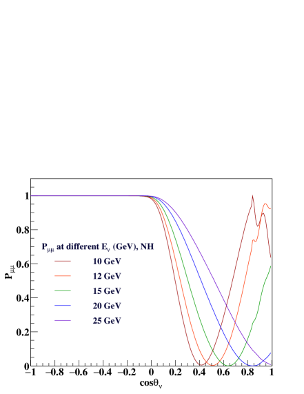
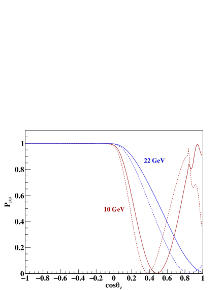
Figure 1: Left: Oscillation probability $P_{\mu\mu}$ as a function of zenith angle for different values of neutrino energy, $E_{\nu}=10,12,15,20,25$ GeV assuming true hierarchy as normal. Right: The same probability shown as solid (dashed) lines for two different energy values for $\Delta m^{2}_{\rm eff}=2.1~{}(2.6)\times 10^{-3}$ eV² to show the sensitivity to this parameter at higher energies.

3.3 The binning scheme

This is similar to, and an extension of, the one used in the earlier analyses [10]. The observables in the analysis are the observed (i.e., smeared) muon energy $E^{obs}_{\mu}$, observed muon direction $\cos\theta^{obs}_{\mu}$ and observed hadron energy $E^{\prime obs}_{had}$, where the true total hadron energy is defined as [10] $E^{\prime}_{had}\equiv E_{\nu}-E_{\mu}$. There are two different analysis sets, one in which only the muon energy and direction, $(E^{obs}_{\mu},\cos\theta^{obs}_{\mu})$, are used, called the 2D (mu only) binning scheme and the other in which all the three observables $(E^{obs}_{\mu},\cos\theta^{obs}_{\mu},E^{\prime obs}_{had})$ are used, which is also known as the 3D (or with-hadron) binning scheme. The details of the two binning schemes are shown in Table 2.

Observable	Range	Bin width	No.of bins
	[0.5, 4]	0.5	7
	[4, 7]	1	3
$E^{obs}_{\mu}$ (GeV)	[7, 11]	4	1
(15 bins)	[11, 12.5]	1.5	1
	[12.5, 15]	2.5	1
	[15, 25]	5	2
	[-1.0, 0.0]	0.2	5
$\cos\theta^{obs}_{\mu}$	[0.0, 0.4]	0.10	4
(21 bins)	[0.4, 1.0]	0.05	12
	[0, 2]	1	2
$E^{\prime obs}_{had}$ (GeV)	[2, 4]	2	1
(4 bins)	[4, 15]	11	1

Table 2: Bins of the three observables, muon energy and direction and hadron energy, used in the analysis.

It should be noted that in the current analysis the direction $\cos\theta^{obs}_{\mu}=+1$ is taken as the up direction. Since atmospheric neutrino oscillations are mainly in the up direction, more bins are assigned in this region than in the down direction. The $E^{obs}_{\mu}$ bins upto 1–11 GeV are taken to be same as those used in Ref. [10]. A bin of width 0.5 GeV is added in the lower energy range. In the higher range of $E^{obs}_{\mu}$, four bins are added, two of them with bin width each of 1.5 GeV and 2.5 GeV respectively and the last two bins of width 5 GeV, thus making the total number of bins in $E^{obs}_{\mu}$ 15. The $\cos\theta^{obs}_{\mu}$ bins and the $E^{\prime obs}_{had}$ are kept the same as in Ref. [10]. Thus same bins are used in the overlapping energy range, and the additional bin sizes were optimised to obtain reasonable event rate as well as sensitivity to oscillation parameters. This gives an optimised result on the whole.

As mentioned above, the number of hadron bins was retained as before, as also the energy range. No extension of hadron energies beyond $E^{\prime obs}_{had}=15$ GeV was used, since this gave only a marginal improvement in $\chi^{2}$ while ICAL’s sensitivity to hadrons at higher energies in terms of the number of hits in the detector tends to saturate [26].

3.4 Number of events

The true number of oscillated events is given by:

$$N_{\mu^{-}} = N_{\mu^{-}}^{0}\times P_{\mu\mu}+N_{e^{-}}^{0}\times P_{e\mu}~{},$$

$$N_{\mu^{+}} = N_{\mu^{+}}^{0}\times\overline{P}_{\mu\mu}+N_{e^{+}}^{0}\times\overline{P}_{e\mu}~{},$$

where $P_{\alpha\beta}$ is the oscillation probability of a flavour $\alpha$ to a flavour $\beta$, $N_{\mu^{\pm}}^{0}$ and $N_{e^{\pm}}^{0}$ refer to unoscillated muon and swapped-muon events generated by NUANCE arising from survived atmospheric $\nu_{\mu}\to\nu_{\mu}$ and oscillated atmospheric $\nu_{e}\to\nu_{\mu}$ interactions in ICAL corresponding to the two terms in Eq. 1.

The number of events per bin including the charge misidentified ones is given as,

$$N^{tot}_{\mu^{-}}(E^{obs}_{\mu},\cos\theta^{obs}_{\mu}) = N_{\mu^{-}}\epsilon_{rec}\epsilon_{cid}+N_{\mu^{+}}\epsilon_{rec}(1-\epsilon_{cid})~{},$$ (5)

$$N^{tot}_{\mu^{+}}(E^{obs}_{\mu},\cos\theta^{obs}_{\mu}) = N_{\mu^{+}}\epsilon_{rec}\epsilon_{cid}+N_{\mu^{-}}\epsilon_{rec}(1-\epsilon_{cid})~{},$$

where $N^{tot}_{\mu^{-}}$ ($N^{tot}_{\mu^{+}}$) is the total number of oscillated $\nu_{\mu}$ ($\overline{\nu}_{\mu}$) CC muon neutrino events observed in the bin $(E^{obs}_{\mu},\cos\theta^{obs}_{\mu})$. The quantity $\epsilon_{rec}$ is the reconstruction efficiency of muons with a given energy and direction and $\epsilon_{cid}$ is the relative charge identification efficiency of the same. The reconstruction and charge identification efficiencies for $\mu^{-}$ and $\mu^{+}$ have been taken to be the same; studies show [23] that they are only marginally different in a few energy-$\cos\theta$ bins. Finally, the events in a bin are considered non-zero if there is at least one event in that bin.

Now this 1000 year sample, oscillated according to the central values of the oscillation parameters listed in Table 1, is scaled to the required number of years to generate the “data”. The current precision analysis is done for 10 years of exposure of 50 kton ICAL (500 kton year). In order to generate the “theory” for comparison with “data” for the $\chi^{2}$ analysis, the oscillation parameters are changed within their $3\sigma$ ranges and the aforementioned processes are repeated. Different theories are generated by changing the oscillation parameters.

4 $\chi^{2}$ analysis

Systematic uncertainties play a very important role in determining the sensitivity to oscillation parameters in any experiment. The inclusion of these uncertaines always gives a worse $\chi^{2}$ than the one obtained when we have no uncertaines at all.

In this new analysis, an extra systematic uncertainty compared to the older analyses is included: the uncertainty on the neutrino–antineutrino flux ratio. This has been considered for the first time in such an analysis and will be seen to have a great impact because ICAL is a magnetised detector that can separate $\mu^{-}$ and $\mu^{+}$ events. With the inclusion of this uncertainty, the $\chi^{2}$ can no longer be expressed as a sum of the separate contributions of neutrino and anti-neutrino events. When the systematic errors are implemented using the usual method of pulls [28, 29, 30, 31, 32] we have,

$$\chi^{2}_{11} = {\stackrel{{\scriptstyle\hbox{min}}}{{\displaystyle\xi_{l}^{\pm},\xi_{6}}}}\sum^{N_{E^{obs}_{\mu}}}_{i=1}\sum^{N_{\cos\theta^{obs}_{\mu}}}_{j=1}\left(\sum^{N_{E^{\prime obs}_{had}}}_{k=1}\right)2\left[\left(T^{+}_{ij(k)}-D^{+}_{ij(k)}\right)-D^{+}_{ij(k)}\ln\left(\frac{T^{+}_{ij(k)}}{D^{+}_{ij(k)}}\right)\right]+$$ (6)

$$2\left[\left(T^{-}_{ij(k)}-D^{-}_{ij(k)}\right)-D^{-}_{ij(k)}\ln\left(\frac{T^{-}_{ij(k)}}{D^{-}_{ij(k)}}\right)\right]+\sum^{5}_{l^{+}=1}\xi^{2}_{l^{+}}+\sum^{5}_{l^{-}=1}\xi^{2}_{l^{-}}+\xi^{2}_{6}~{},$$

where $i,j,k$ sum over muon energy, muon angle and hadron energy bins. The number of theory (expected) events in each bin, with systematic errors, is given by,

$$T^{+}_{ij(k)} = T^{0+}_{ij(k)}\left(1+\sum^{5}_{l^{+}=1}\pi^{l^{+}}_{ij(k)}\xi_{l^{+}}+\pi_{6}\xi_{6}\right)~{},$$ (7)

$$T^{-}_{ij(k)} = T^{0-}_{ij(k)}\left(1+\sum^{5}_{l^{-}=1}\pi^{l^{-}}_{ij(k)}\xi_{l^{-}}-\pi_{6}\xi_{6}\right)~{},$$

where $T^{0\pm}_{ij(k)}$ is the corresponding number of events without systematic errors, $D^{\pm}_{ij(k)}$ is the number of “data” (observed) events in each bin, and $\xi_{l^{\pm}}$ are the pulls corresponding to the same five systematic uncertainties, $l=1,\ldots,5$, for each of neutrino and anti-neutrino contributions, as considered in the earlier analyses by the INO collaboration [1, 8, 9, 10].

The five systematic uncertaines include the flux normalisation, shape (spectral or energy dependence) uncertainty or “tilt” and zenith angle uncertainties, the cross-section unertainties, and an overall systematic uncertainty due to the detector response (see Ref. [10] for details).

The cross-section uncertainty is assumed to be process independent. At high energies, the cross-section is dominated by deep inelastic scattering (DIS) where the uncertainties are smaller; however, in the energy range of interest here, all processes (quasi-elastic (QE), resonance (RES) and DIS) have significant contributions and so a common cross-section uncertainty is used.

Here the values of $\pi^{l}$ are taken to be the same for neutrino events and anti-neutrino events; i.e, $\pi^{l\pm}\equiv\pi^{l};l=1,\ldots,5$. The values used in this analysis are the same as those used in the earlier analysis by the INO collaboration [8, 9, 10, 1]:

1. $\pi_{1}=20$% flux normalisation error,

2. $\pi_{2}=10$% cross section error,

3. $\pi_{3}=5$% tilt error,

4. $\pi_{4}=5$% zenith angle error,

5. $\pi_{5}=5$% overall systematics.

In Eq. 6 $\xi_{6}$ is the 11th (additional) pull and $\pi_{6}$ is taken to be 2.5%. The effect of the new pull can be understood by considering its contribution alone on the ratio of neutrino to anti-neutrino events:

$$\frac{N^{+}}{N^{-}} \simeq \frac{T^{0+}}{T^{0-}}\frac{(1+\pi_{6}\xi_{6})}{(1-\pi_{6}\xi_{6})}$$ (8)

$$\simeq \frac{T^{0+}}{T^{0-}}(1+2\pi_{6}\xi_{6})~{}.$$ (9)

This pull therefore accounts for the uncertainty in the flux ratio; $2\pi_{6}$ corresponds to the 1$\sigma$ error (when $\xi_{6}=1$); this gives the 1$\sigma$ error on the ratio to be 5%, consistent with Ref. [18, 33]. In the earlier analysis with 10 pulls only, the pulls for $N^{-}$ and $N^{+}$ were independent so that they could be in the same or opposite directions. The introduction of the 11th pull constrains the ratio and results in a (negative) correlation between the normalisations of the $T^{+}$ and $T^{-}$ events, as will become clear from the discussions presented in Sections 5 and 6. Without this pull, the total $\chi^{2}$ can be simply expressed as a sum over the $\mu^{-}$ and $\mu^{+}$ contributions :

$$\chi^{2}_{10}=\chi^{2}_{+}+\chi^{2}_{-}.$$ (10)

Note that the observed muon events have contributions from both the $\Phi_{\mu}$ and $\Phi_{e}$ fluxes; here we have assumed the same systematic error on both the $\overline{\Phi}_{\mu}/\Phi_{\mu}$ and $\overline{\Phi}_{e}/\Phi_{e}$ ratios (although, in principle, this can be included separately). We have also ignored the small differences due to additional possible uncertainty in the $\Phi_{\mu}/\Phi_{e}$ flux ratios since the contribution from the second term in Eq. 1, i.e., from $\nu_{e}\to\nu_{\mu}$ oscillations is subdominant/small.

An 8% prior at 1$\sigma$ is also added on $\sin^{2}2\theta_{13}$, since this quantity is known to this accuracy [4, 5]. No prior is imposed on $\theta_{23}$ and $\Delta{m_{32}^{2}}$, since the precision measurements of these parameters are to be carried out with ICAL. The contribution to $\chi^{2}$ due to prior is defined as :

$$\chi_{\rm prior}^{2}=\left(\frac{\sin^{2}2\theta_{13}-\sin^{2}2\theta_{13}^{\rm true}}{\sigma(\sin^{2}2\theta_{13})}\right)^{2}~{},$$ (11)

where $\sigma(\sin^{2}2\theta_{13})$ = $0.08\times\sin^{2}\theta_{13}^{\rm true}$. Thus the total $\chi^{2}$ is defined as:

$$\chi_{\rm ICAL}^{2}=\chi^{2}+\chi_{\rm prior}^{2}~{},$$ (12)

where $\chi^{2}$ corresponds suitably to $\chi^{2}_{11}$ (new analysis) or $\chi^{2}_{10}$ (repeat of the older analysis with extended energy range).

During $\chi^{2}$ minimisation, $\chi_{\rm ICAL}^{2}$ is first minimised with respect to the pull variables $\xi_{l}$ for a given set of oscillation parameters, then marginalised over the ranges of the oscillation parameters $\sin^{2}\theta_{23}$, $\Delta m^{2}_{\rm eff}$ and $\sin^{2}2\theta_{13}$ given in Table 1. The third column of the table shows the 3$\sigma$ range over which the parameter values are varied. These along with the best fit values of $\theta_{12}$ and $\Delta{m_{21}^{2}}$ are obtained from the global fits in Refs. [34, 35, 36, 37, 38]. As mentioned earlier, the parameter $\delta_{CP}$ is kept fixed at zero throughout this analysis.

The relative precision achieved on a parameter $\lambda$ (here $\lambda$ being $\sin^{2}\theta_{23}$ or $|\Delta{m^{2}_{\rm eff}}|$) at 1$\sigma$ is expressed as :

$$p(\lambda)=\frac{\lambda_{\hbox{max-}2\sigma}-\lambda_{\hbox{min-}2\sigma}}{4\lambda_{true}}~{},$$ (13)

where $\lambda_{\hbox{max-}2\sigma}$ and $\lambda_{\hbox{min-}2\sigma}$ are the maximum and minimum allowed values of $\lambda$ at 2$\sigma$; $\lambda_{true}$ is the true choice.

The statistical significance of the obtained result is denoted by $n\sigma$, where, $n=\sqrt{\Delta\chi^{2}}$, which is given by:

$$\Delta\chi^{2}(\lambda)=\chi^{2}_{ICAL}(\lambda)-\chi^{2}_{0}~{},$$ (14)

$\chi^{2}_{0}$ being the minimum value of $\chi^{2}_{ICAL}$ in the allowed parameter range. With no statistical fluctuations, $\chi^{2}_{0}=0$.

5 Results: precision measurement of parameters

The precision measurement of oscillation parameters in the atmospheric sector in the energy range 0.5–25 GeV is probed in the current analysis using 500 kton year exposure of ICAL detector. Comparisons with previous analyses in the 1–11 GeV energy range are also done to illustrate how much better is the sensitivity with our new analysis. Sensitivities to the oscillation parameters $\theta_{23}$ and $|\Delta{m_{\rm eff}^{2}}|$ are found separately, when the other parameter and $\theta_{13}$ are marginalised over their 3$\sigma$ ranges. Marginalisation is also done over the two possible mass hierarchies; since atmospheric neutrino events in ICAL are sensitive to the mass hierarchy (also discussed below), the wrong hierarchy always gives a worse value of $\chi^{2}$ during marginalisation. Typically, normal hierarchy (NH) is taken to be the true hierarchy (a couple of results with inverted hierarchy (IH) are shown for completeness) and 500 kton years of exposure is used (10 years of running the experiment).

5.1 Precision measurement of $\sin^{2}\theta_{23}$

The relative 1$\sigma$ precision on $\sin^{2}\theta_{23}$ obtained from different analyses, with normal hierarchy as the true hierarchy, is shown in Fig. 2 for different cases which are the combinations of energy ranges, binning schemes and number of pulls.

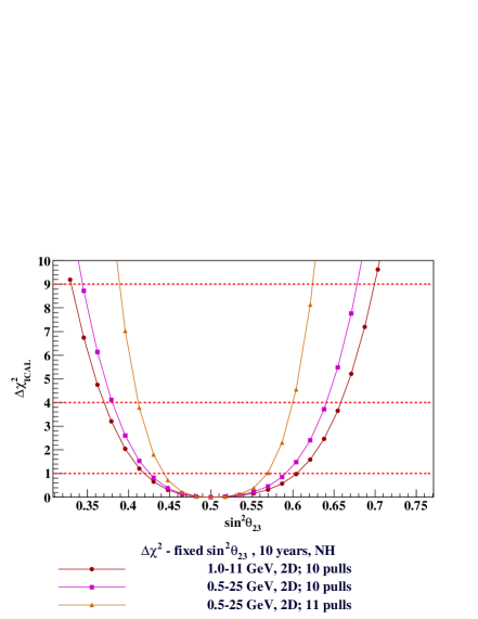
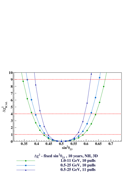
Figure 2: $\Delta\chi^{2}_{\rm ICAL}$ at different values of $\sin^{2}\theta_{23}$ with true $\sin^{2}\theta_{23}=0.5$ and with normal hierarchy as the true hierarchy. The left panel shows the results for muon only (2D) analysis and the right panel shows those for the analysis with hadrons also (3D), for all possible combinations of energy ranges, pulls and binning schemes.

The other parameters $|\Delta{m^{2}_{\rm eff}}|$ and $\theta_{13}$ have been marginalised over their 3$\sigma$ ranges as given in Table 1. Percentage precisions on $\sin^{2}\theta_{23}$ at 1$\sigma$ obtained with different analyses are shown in Table 3.

Binning	$E^{obs}_{\mu}$ (GeV)	No.of pulls	$\sin^{2}\theta_{23_{min}}$	$\sin^{2}\theta_{23_{max}}$	Precision
			at 2$\sigma$	at 2$\sigma$	at 1$\sigma$ (%)
	1–11	10	0.370	0.658	14.40
2D (NH)	0.5–25	10	0.380	0.640	13.00
$(E^{obs}_{\mu},\cos\theta^{obs}_{\mu})$	0.5–25	11	0.412	0.599	9.35
	1–11	10	0.381	0.639	12.85
3D (NH)	0.5–25	10	0.394	0.619	11.25
$(E^{obs}_{\mu},\cos\theta^{obs}_{\mu},E^{\prime obs}_{had})$	0.5–25	11	0.416	0.594	8.90
3D (IH)	0.5–25	11	0.421	0.606	9.25
$(E^{obs}_{\mu},\cos\theta^{obs}_{\mu},E^{\prime obs}_{had})$

Table 3: Precision of $\sin^{2}\theta_{23}$ at 1$\sigma$, obtained using Eq. 13, from different analyses. The maximum and minimum values of $\sin^{2}\theta_{23}$ at 2$\sigma$ in each case are also shown. The true value of $\sin^{2}\theta_{23}$ is taken to be 0.5 with normal hierarchy as the true hierarchy. The last row shows the precision with IH as the true hierarchy.

2D Analysis of $\sin^{2}\theta_{23}$

: The extension of the $E^{obs}_{\mu}$ range to 0.5–25 GeV improves the precision to 13% from 14% obtained in the earlier analysis with 1–11 GeV [8, 10]. A very large enhancement in precision to 9% is obtained when the 11^th pull is included. This is a very significant observation for all magnetised detectors and the reason for this improvement is discussed in Section 6.

3D Analysis of $\sin^{2}\theta_{23}$

: A similar result of 9% precision is obtained with the 3D analysis. This is better than the earlier result of 13% [10]. The 2D muon-only analysis gives a comparable result; this is significant because the muon-only analysis avoids the problem of the large uncertainties arising from the mis-identification of hadron hits as muon hits in the detector (and vice versa). Of course an improved measurement of hadron energy can further improve this result.

The earlier best result (with 1–11 GeV in muon energy, hadron bins as listed in Table 2, and including only 10 pulls) [10] is shown in comparison with the best results of the present analysis (using 0.5–25 GeV in muon energy, the same hadron bins, but with 11 pulls) in Fig. 3 (left) for NH. Indeed, it can be seen that the earlier best result to $3\sigma$ precision is worse than that already known from other experiments as listed in Table 1. The precision obtainable with IH as the true hierarchy was also studied with our latest analysis. The relative 1$\sigma$ precision obtained with IH is 9.25% which is comparable to that obtained from NH (8.9%), as can be seen in Fig. 3 (right). This is comparable to or slightly better than the precision on $\sin^{2}\theta_{23}$ obtained by T2K [39, 40, 41]. That is, the 11^th pull acts as a constraint on the relative $\mu^{+}$ and $\mu^{-}$ events so that a magnetised atmospheric neutrino detector can achieve the precision obtained by an accelerator experiment. We believe that this fact has been pointed out for the first time in this paper.

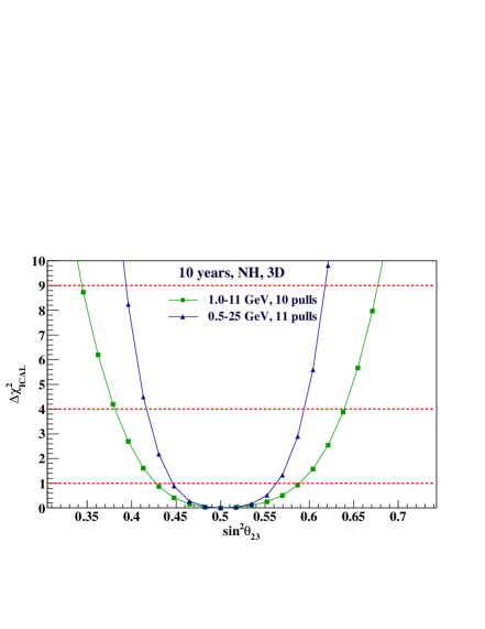
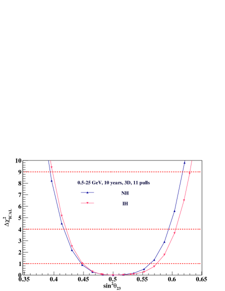
Figure 3: Left: The best precision on $\sin^{2}\theta_{23}$ obtained from the current in comparison with earlier [10] 3D simulations analyses of ICAL, including information from hadrons, assuming normal hierarchy as the true one. Right: The best precision on $\sin^{2}\theta_{23}$ obtained from the current analysis for both hierarchies. For details see text.

5.2 Precision on $|\Delta{m^{2}_{32}}|~{}(|\Delta{m^{2}_{31}}|)$

Since ICAL is a magnetised iron calorimeter, it can measure $|\Delta{m^{2}_{32}}|$ with very good precision. As in the case of $\sin^{2}\theta_{23}$, there are six different analyses which give the results as shown in Fig. 4. The percentage precisions at $1\sigma$ obtained for the magnitude of $\Delta{m^{2}_{32}}~{}(\Delta{m^{2}_{31}})$ are shown in Table 4 when the true hierarchy is normal (inverted). It can be seen that ICAL will be able to determine $|\Delta{m^{2}_{32}}|~{}(|\Delta{m^{2}_{31}}|)$ with a greater precision than $\sin^{2}\theta_{23}$, in all energy ranges.

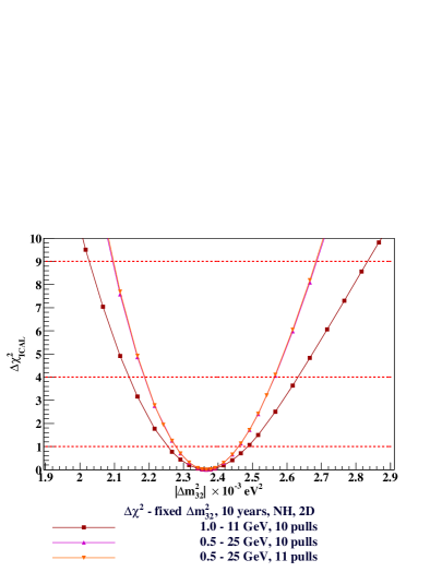
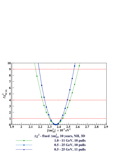
Figure 4: Precision on $|\Delta{m_{32}^{2}}|$ with true $|\Delta{m_{32}^{2}}|=2.366\times 10^{-3}~{}{\rm eV}^{2}$ ($|\Delta{m_{\rm eff}^{2}}|=2.4\times 10^{-3}~{}{\rm eV}^{2}$) with normal hierarchy as the true hierarchy. The left panel shows the results for the 2D analyses and the right one shows those for the 3D analyses. The results for all possible combinations of energy ranges, pulls and binning schemes are shown.

The current best results with 2D and 3D analyses are shown in Fig. 5 (left). The new 2D and 3D analyses in the range $E^{obs}_{\mu}$ = 0.5–25 GeV constitute an improvement over the older 2D and 3D analyses [10]. However, as the precision on $|\Delta{m^{2}_{32}}|$ achievable by ICAL is alreay quite good, the improvement does not seem to be as pronounced as in the case of the case of $\sin^{2}\theta_{23}$ although the 3D analysis is itself an improvement over the current bounds.

2D Analysis of $|\Delta{m^{2}_{32}}|$

: The muon-only (2D) analysis with 10 pulls gives a precision of 4%, which is a $\sim$ 22% improvement over the old value. With the additional constraint of the 11^th pull in the $E^{obs}_{\mu}$ = 0.5–25 GeV case, the precision achievable is similar, which shows that the new pull does not improve the precision further. This is in contrast to the precision measurement of $\sin^{2}\theta_{23}$, the precision of which is impacted mainly by the constraint on the $\nu_{\mu}$-$\overline{\nu}_{\mu}$ flux ratio.The reason for this is discussed in Section 6.

3D Analysis of $|\Delta{m^{2}_{32}}|$

: The precision obtained with 3D binning and 10 pulls in 0.5–25 GeV improves to 2.5% from the older value of 3%, which corresponds to a $\sim$ 17% increase. The addition of the 11^th pull again does not improve the precision further. Precision measurement with IH as the true hierarchy gives a precision which is comparable to that obtained for NH. This is shown in the right panel of Fig. 5, where the $x$-axis corresponds to $\Delta{m^{2}_{32}}$ for NH and $(-\Delta{m^{2}_{31}})$ for IH.

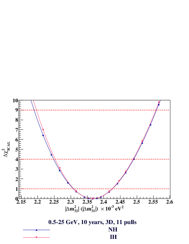
Figure 5: Left: Comparison of $\Delta\chi^{2}_{ICAL}$ obtained from 2D and 3D analyses in the energy range $E^{obs}_{\mu}$ = 0.5–25 GeV and with 11 pulls with normal hierarchy as the true one. The best result is for the 3D analysis (which is similar with either 10 or 11 pulls. Right: Best sensitivity to $|\Delta{m^{2}_{32}}|$ in the current analysis (3D, 11 pulls) for both normal and inverted hierarchies.

Binning	$E^{obs}_{\mu}$ (GeV)	No.of pulls	$|\Delta{m^{2}_{32(1)}}|_{min}$	$|\Delta{m^{2}_{32(1)}}|_{max}$	Precision
			$\times 10^{-3}{\rm eV}^{2}$ at 2$\sigma$	$\times 10^{-3}{\rm eV}^{2}$ at 2$\sigma$	at 1$\sigma$ (%)
	1–11	10	2.142	2.630	5.15
2D	0.5–25	10	2.186	2.565	4.00
$(E^{obs}_{\mu},\cos\theta^{obs}_{\mu})$	0.5–25	11	2.188	2.563	3.96
	1–11	10	2.224	2.517	3.09
3D	0.5–25	10	2.248	2.491	2.57
$(E^{obs}_{\mu},\cos\theta^{obs}_{\mu},E^{\prime obs}_{had})$	0.5–25	11	2.248	2.491	2.57
3D (IH)	0.5–25	11	2.253	2.488	2.48
$(E^{obs}_{\mu},\cos\theta^{obs}_{\mu},E^{\prime obs}_{had})$

Table 4: Precision of $|\Delta{m^{2}_{32}}|~{}(|\Delta{m^{2}_{31}}|)$ at 1$\sigma$, obtained using Eq. 13, from different analyses. The maximum and minimum values of $|\Delta{m^{2}_{32}}|~{}(|\Delta{m^{2}_{31}}|)$ at 2$\sigma$ in each case are also shown. The true value of $|\Delta{m^{2}_{32}}|~{}(|\Delta{m^{2}_{31}}|)$ is taken to be $|\Delta{m^{2}_{32}}|~{}(|\Delta{m^{2}_{31}}|)=2.366\times 10^{-3}$ eV² ($|\Delta{m^{2}_{\rm eff}}|=2.4\times 10^{-3}{\rm eV}^{2}$) with normal (inverted) hierarchy as the true hierarchy.

5.3 Simultaneous precision on $\sin^{2}\theta_{23}$ and $|\Delta{m^{2}_{32}}|$

The results discussed in the previous sections were for fixed values of either of the oscillation parameters $\sin^{2}\theta_{23}$ and $|\Delta{m^{2}_{32}}|~{}(|\Delta{m^{2}_{31}}|)$. We now discuss the parameter space allowed by our latest analysis. The analysis was done for the 11 pull case with $E^{obs}_{\mu}$ = 0.5–25 GeV and with hadrons, for 500 kton yrs of ICAL exposure. Normal hierarchy is assumed to be the true hierarchy.

The 90% and 99% confidence contours for 500 kton year exposure of ICAL for NH with the true choices of $(\sin^{2}\theta_{23},|\Delta{m^{2}_{32}}|)=(0.5,2.366\times 10^{-3}{\rm eV}^{2}))$ are shown in the left panel of Fig. 6. Similar results hold true for inverted hierarchy as the true hierarchy. It can be seen that the extension of the energy range for analysis and constraining the $\nu_{\mu}-\overline{\nu}_{\mu}$ flux ratio in ICAL result in an improved sensitivity to the precision on both parameters. The projected ICAL precision on $\sin^{2}\theta_{23}$ is better than or comparable to the current T2K precision as can be seen from the right panel of Fig. 6, where the 90% CL contour is compared to the results from T2K [42]. A comparison of these projected results for ICAL (NH) with the current results from MINOS [43] and T2K [42] are shown in Fig. 7. It must be remembered, though, that these experiments are already taking data while ICAL is yet to be constructed!

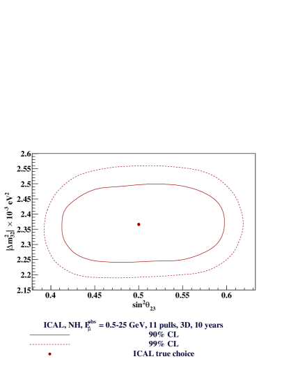
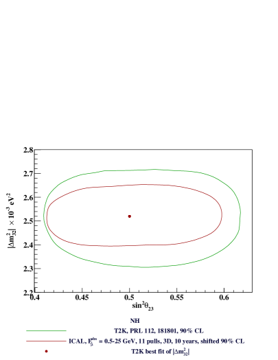
Figure 6: (Left) Allowed contours at 90% and 99% confidence level for 500 kton yr exposure of ICAL in the $\sin^{2}\theta_{23}-|\Delta{m^{2}_{32}}|$ plane. The red dot shows the true choice of parameters for the ICAL analysis, $(\sin^{2}\theta_{23},|\Delta{m^{2}_{32}}|)=(0.5,2.366\times 10^{-3}{\rm eV}^{2})$ with NH. (Right) Comparison of the ICAL projected 10 year sensitivity with the current T2K result at 90% CL. The ICAL contour is shifted to match the best-fit value of $|\Delta m^{2}_{32}|$ from T2K [42].

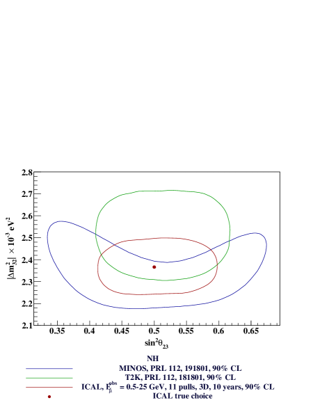
Figure 7: The $\Delta\chi^{2}_{ICAL}$ contours at 90% C.L. in the $\sin^{2}\theta_{23}$–$|\Delta m^{2}_{32}|$ plane for 500 kton yrs exposure of ICAL (3D analysis with $E^{obs}_{\mu}$ = 0.5–25 GeV and the inclusion of the 11th pull). The 90% confidence contours from MINOS [43] and T2K [42] are also shown for comparison. The red dot shows the true choice of parameters for the ICAL analysis, $(\sin^{2}\theta_{23},|\Delta{m^{2}_{32}}|)=(0.5,2.366\times 10^{-3}{\rm eV}^{2})$.

5.4 Sensitivity to neutrino mass ordering

ICAL with its magnetisability is an exclusive mass hierarchy machine. Most importantly, its ability to discriminate the normal and inverted mass ordering is independent of the CP phase [1]. The ability of ICAL to distinguish the correct mass ordering in the 2–3 sector is given by :

$$\Delta\chi^{2}_{MO\hbox{-}ICAL}=\chi^{2}_{false\hbox{-}MO}-\chi^{2}_{true\hbox{-}MO}~{},$$ (15)

where $\chi^{2}_{false\hbox{-}MO}$ is the minimum $\chi^{2}$ calculated using the false ordering, while allowing $\theta_{23}$, $\theta_{13}$ and $|\Delta m^{2}_{\rm eff}|$ to vary over the $3\sigma$ range given in Table 1 and $\chi^{2}_{true-MO}$ is the minimum $\chi^{2}$ assuming the true mass ordering. The plot of $\Delta\chi^{2}_{MO\hbox{-}ICAL}$ as a function of the number of years of exposure is shown in Fig. 8 both when the true ordering is taken to be normal (NO) as well as inverted (IO).

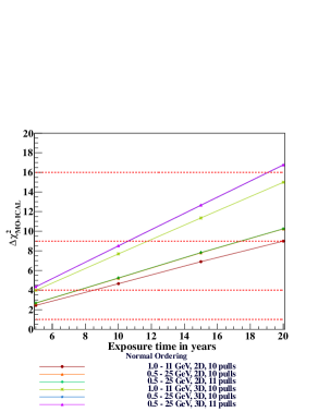
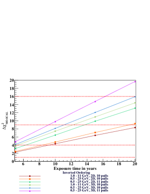
Figure 8: $\Delta\chi^{2}_{MO\hbox{-}ICAL}$ as a function of exposure time in years. The extension of observed muon energy range to 0.5–25 GeV increases the sensitivities in the case of both 2D and 3D. The extra pull improves the hierarchy sensitivity when the true ordering is inverted.

Normal Ordering: The muon-only analysis (2D) with 10 pulls only gives a $\Delta\chi^{2}_{MO\hbox{-}ICAL}$ of $\sim$ 5.2 for 10 years of ICAL exposure, better than the earlier result of $\sim$ 4.6, a 13% increase in the hierarchy sensitivity. Again the addition of the 11th pull does not improve $\Delta\chi^{2}_{MO\hbox{-}ICAL}$ in both energy ranges in the 2D analysis.

The addition of hadron energy as the third observable increases the $\Delta\chi^{2}_{MO\hbox{-}ICAL}$ to $\sim 8.5$, for an exposure time of 10 years, an improvement over the earlier value of 7.7. Again the addition of the 11th pull has no effect on the hierarchy sensitivity when normal ordering is taken to be the true ordering.

Inverted ordering: While trends are similar to that with normal order as the true order, the inclusion of the 11th pull has significant impact on mass hierarchy sensitivity when the true ordering is inverted. In fact, the best sensitivity ($E^{obs}_{\mu}$ = 0.5–25 GeV, with 11 pulls and 3D binning) is better with the inverted than with the normal hierarchy (by $\sim$ 16%). The reason for this effect with the 11^th pull is discussed in the next section.

It should be noted that the values of $\Delta\chi^{2}_{MO\hbox{-}ICAL}$ are lower than those reported in Ref. [10], for the same exposure time. This is due to the fact that the earlier analysis used the input value $\theta_{13}\sim 9.217^{\circ}$ while our analysis uses the current best fit value [44] $\theta_{13}\sim 8.729^{\circ}$. Given that the best fit of $\theta_{13}$ has reduced further to $\sim 8.5^{\circ}$ [34, 45] it is even more important to perform the analysis in as wide a kinematic range (energy and direction) as possible to get the best possible hierarchy discrimination.

5.4.1 Dependence on $\theta_{23}$

The sensitivity to mass ordering is also known to depend on the true value of $\theta_{23}$; it is higher for larger $\theta_{23}$ as can be seen from Fig. 9. While ICAL has better sensitivity to the inverted ordering when $\theta_{23}$ is in the first octant, the reverse is true when it is in the second octant. This is due to the dominance of the $P_{\mu\mu}$ term in Eq. 1 arising from the survived $\nu_{\mu}$s compared to the $P_{e\mu}$ term from oscillated $\nu_{e}$s, and the nature of its dependence on $\theta_{23}$. In fact, the results would also be vastly improved by “switching off” the $P_{e\mu}$ term since their dependence on the oscillation parameters (especially $\theta_{23}$) are practically the opposite of each other [20]. This is not possible with atmospheric neutrinos where Nature provides both flavours, but is possible with neutrino beams. In the latter case, however, the fact that there is a single base-line which results in a significant dependence on and correlation with the CP violating phase $\delta_{CP}$ and complicates the analysis, as with MINOS [43], T2K [39], LBNE [46, 47] or NO$\nu$A [9, 48].

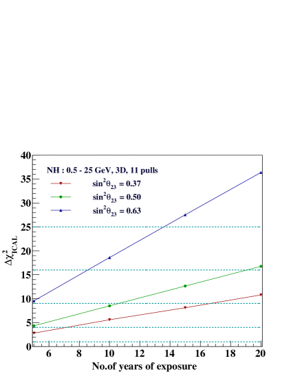
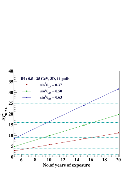
Figure 9: The best case values of $\Delta\chi^{2}_{MO\hbox{-}ICAL}$ as a function of exposure time in years. It can be seen that the sensitivity to mass hierarchy increases linearly with the true value of $\theta_{23}$ when it is varied over the $3\sigma$ range of the parameter.

To summarise, the sensitivity to the mass ordering in the 2–3 sector improves with the addition of higher energy bins in the analysis, while constraining the $\nu_{\mu}~{}-~{}\overline{\nu}_{\mu}$ flux ratio improves the sensitivity only when the true ordering is inverted. The ICAL’s ability to determine this mass ordering is significant owing to its magnetisability and its 50 kton mass. Improvement in energy resolutions will further improve the detector’s sensitivity to this parameter. Also, in ICAL, the mass ordering can be determined independent of the CP violating phase $\delta_{CP}$ because of the range of baselines involved in atmospheric neutrinos [1]; this is in contrast to beam/short-base-line experiments where there is a non-trivial sensitivity to the 2–3 mass ordering depending on the true value of the CP phase. Hence ICAL will be important in the determination of this mass ordering, and any amount of improvement in determining this parameter is noteworthy.

6 Impact of the 11^th pull on determination of the oscillation parameters

The 11^th pull accounts for the fact that the ratios of the $\nu_{\mu}$ and $\overline{\nu}_{\mu}$ fluxes are better known (to within 5%) than the absolute fluxes themselves [18]. This is implemented by using a pull $\pi_{6}=0.025$, which contributes with the opposite sign for neutrino and anti-neutrino events, as can be seen from Eq. 9.

It is seen that the inclusion of the 11th pull is most visible in the determination of $\theta_{23}$ which becomes more constrained when this pull is included. One way to understand this is to re-bin the events in a single variable $L/E$ (of the final state muon) and consider the effect of just this pull. Fig. 10 shows the effect of $\theta_{23}$ on both the neutrino and anti-neutrino events. The thick solid line is the “data” corresponding to $\theta_{23}=45^{\circ}$ while the thin solid “theory” line corresponds to a fit with $\theta_{23}=40^{\circ}$ and without any pull. In both cases, reducing $\theta_{23}$ from the true value increases the event rate in every bin (the opposite will hold with the inverted hierarchy; here the normal hierarchy is shown). Note that the down-going events are not shown here.

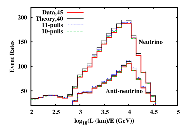
Figure 10: The 10 year rates from CC $\nu_{\mu}$ and $\overline{\nu}_{\mu}$ events shown as a function of $\log_{10}(L(\hbox{km})/E(\hbox{GeV}))$ of the final state muon. The red (thick solid) lines correspond to the “data” and the black (thin solid) ones to the “theory” with $\theta_{23}=40^{\circ}$ (and other parameters held fixed). The green (dashed) lines (practically overlapping the data) and the blue (dot-dashed) lines mimic the effect of 10th pull and inclusion of the 11th pull respectively.

The dot-dashed and dashed curves corresponding to the labels 11- and 10-pulls show the effect of changing the (single) normalisation of the theory with and without the 11^th pull. The overall normalisation of the events in the 10-pull case can be independently varied for neutrinos and anti-neutrinos (decreased by 4% and 3% in figure) to improve the agreement of the $40^{\circ}$ theory line to the data, resulting in smaller overall $\chi^{2}$ in this fit. On the other hand, a 2.5% decrease in the normalisation of neutrino-induced events in the 11-pull case is accompanied by a 2.5% increase in the anti-neutrino case, so that the agreement with the neutrino data becomes better, but that with the anti-neutrino data becomes worse. (Of course, it can be applied vice versa, but the smaller $\chi^{2}$ is obtained with this choice since there are about twice as many neutrino events as anti-neutrino ones due to the smaller cross section of the latter.) Hence it is not possible to improve the agreement of the $40^{\circ}$ theory with data by tuning the normalisation in the analysis when including this pull; this results in a larger $\chi^{2}$ compared to the 10-pull case where the normalisations of neutrino- and anti-neutrino-induced events can be independently varied. This gives rise to the tighter constraints on $\theta_{23}$ when the 11th pull is added. We note that only a detector like ICAL that is capable of charge identification can successfully implement this pull as a constraint.

It can also be seen from Fig. 10 that there is greater sensitivity to $\theta_{23}$ in the neutrino rather than in the anti-neutrino sector. The reverse is true with inverted mass ordering. In the determination of the sensitivity to the mass ordering, the minimum $\chi^{2}$ with the false ordering is found. That means, when the true ordering is inverted, the “theory” is obtained using the normal ordering, where there is greater sensitivity to $\theta_{23}$ as just mentioned. When the 11th pull is included, therefore, the discrepancy between theory and data cannot be achieved by changing $\theta_{23}$ and hence there is more sensitivity to determination of the mass ordering when the true ordering is inverted, provided $\theta_{23}$ is in the first octant. The reverse is true when $\theta_{23}$ is in the second octant, as can be seen from Fig. 9.

In addition, it can be seen from Fig. 10 that there is sensitivity to oscillation parameters near and beyond $\log_{10}(L({\rm km})/E({\rm GeV}))\sim 4$. This is precisely the region that is included when the range of $E^{obs}_{\mu}$ is extended from 1 GeV down to 0.5 GeV. Similarly, although smaller, sensitivity to the parameters is also seen for $\log_{10}(L({\rm km})/E({\rm GeV}))\sim 2$–3, which corresponds to the extension in the higher energy end from 11 to 25 GeV.

7 Summary and Discussion

This paper contains a simulation study of the physics potential of the proposed 50 kton magnetised Iron Calorimeter detector (ICAL) at INO which aims to probe neutrino oscillation parameters by observing atmospheric neutrino oscillations and studying their Earth matter effects as they propagate through the Earth. This will be done by detecting (mainly) the charged current interactions of $\nu_{\mu}$ and $\overline{\nu}_{\mu}$ in the detector by means of the final state muons. The detector, which is optimised for the detection of muons in the GeV energy range, will have a magnetic field which will enable the distinction of $\nu_{\mu}$ and $\overline{\nu}_{\mu}$ events by identifying the charge of the muon in the final state, thus making ICAL an excellent detector to determine the neutrino mass ordering. Not only this, the magnetic field helps to improve the precision measurement of the mixing angle $\theta_{23}$ (and $|\Delta{m^{2}_{32}}|$ and the mass ordering as well).

The main themes of our study were the effects of extending the observed muon energy range to 0.5–25 GeV (from 1–11 GeV used in earlier studies) and that of a constraint on the $\nu_{\mu}$–$\overline{\nu}_{\mu}$ flux ratio on the sensitivity of a 50 kton ICAL to neutrino oscillation parameters in the 2–3 sector. The second—and the aspect which is found to have the biggest impact so far on oscillation sensitivity—arises from two facts; one that ICAL detects atmospheric neutrinos and the other that this massive detector will be magnetised.

In particular, we show that the relatively small uncertainties on the atmospheric neutrino-antineutrino flux ratios act as a constraint in analyses where the neutrino and antineutrino events can be separated. This is true in a magnetised detector such as ICAL where the magnetic field distinguishes muons and anti-muons produced in charged current interactions of neutrinos and antineutrinos respectively with the detector material. The presence of the magnetic field enables ICAL to distinguish between neutrino and anti-neutrino events; hence, inclusion of the uncertainty on the $\nu_{\mu}/\overline{\nu}_{\mu}$ flux ratio as an additional pull translates to a constraint on this ratio which in turn significantly improves the precision with which $\sin^{2}\theta_{23}$ can be determined. Such a constraint is applicable for all magnetised detectors which have good charge identification capabilities and the impact of this constraint has been shown for the first time in this paper. As a consequence, our simulation studies show that, with 10 years of data taking, ICAL will not only be able to determine $|\Delta m^{2}_{32}|$ with good precision (as expected) but can also pin down $\sin^{2}\theta_{23}$ to a precision better than the current limits set by T2K.

The precision that can be achieved on these parameters in about 10 years’ running is about 2.5% and 9% for $|\Delta m^{2}_{32}|$ and $\sin^{2}\theta_{23}$ respectively; see details in Tables 3 and 4.

The studies presented here assume that there is perfect separation between different types of charged current (CC) and neutral current (NC) events. The event separation efficiency will affect the results of the analysis since they will determine the actual number of events in each bin apart from the contamination from NC oscillation-independent events. However the inclusion of this consideration is beyond the scope of this paper. Preliminary studies [49] show that certain selection criteria can be applied so that an event sample which comprises more than 95% CC muon events can be obtained. The criterion results in cutting out events with $E_{\nu}\lesssim 0.5$ GeV; this has determined largely the range (lower limit) of muon energy analysed in this paper. Also, improvements in the reconstruction efficiencies and resolutions (that have been studied with GEANT-4 simulations of the detector) as well as possible changes in detector geometry can all alter the results of this analysis. Note that the current studies were all done with the atmospheric neutrino fluxes computed at the Super Kamiokande site [18]. The fluxes at Theni where ICAL is proposed to be built are slightly different and are smaller at energies less than 10 GeV [18, 50]; this will also impact the analysis.

Even within these limitations, it appears that the physics results of ICAL will have the capability to impact global fits to neutrino data and thus any new analysis will open a window to understanding the neutrino oscillation parameters better on the whole and the atmospheric neutrino fluxes themselves, in particular.

Appendix A The effect of fluctuations

As discussed in Section 3.4, the analyses in the previous sections were done by taking a 1000 year sample of charged current muon neutrino events and scaling it down to the required number of years for comparison with “data”. It is important to reduce “theory” fluctuations so as to obtain a genuine result from the analysis. The effect of taking different years of exposure as theory samples, to be scaled to 10 years on precision measurements of $\theta_{23}$ and $|\Delta{m^{2}_{32}}|$, is shown in Fig. 11 for arbitrarily chosen values of $\theta_{23}=39^{\circ}$ and $\Delta m^{2}_{32}=2.466\times 10^{-3}$ eV² ($\Delta m^{2}_{\rm eff}=2.5\times 10^{-3}$ eV²). It can be seen that a smaller sample has more fluctuations and hence yields a larger value of $\Delta\chi^{2}_{ICAL}$ for a given parameter thus giving too good a precision on the oscillation parameter which is false. The larger sample takes care of this by reducing the ($\sqrt{N}$) fluctuations in the theory itself. The $\chi^{2}$ stabilises at a point when the sample is fairly large and this is the number of years of exposure to be taken and scaled down for the analysis. It can be seen that use of 1000 year sample yields fairly stable results and thus the analyses have made use of such a sample of charged current muon neutrino events. We note however that the results are much more sensitive to the sample size in the case of $|\Delta m^{2}_{32}|$ than for $\theta_{23}$.

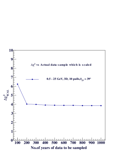
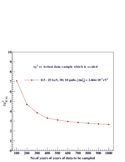
Figure 11: The value of $\Delta\chi^{2}_{ICAL}$ vs the number of years of sample theory to be scaled to 10 years for $\theta_{23}=39^{\circ}$ (left) and $|\Delta{m}_{32}^{2}|=2.466\times 10^{-3}{\rm eV}^{2}$ (right). It can be seen that the scaling of only 100 years of sample size gives too high a $\chi^{2}$ which is more prominent in the case of $\Delta m^{2}_{32}$. As the number of years of sample to be scaled increases, the value of $\chi^{2}$ also comes down as well as saturates for large enough sample sizes.

References

- [1] S Ahmed et al., INO Collaboration, Physics Potential of the ICAL detector at the India-based Neutrino Observatory (INO), INO/ICAL/PHY/NOTE/2015-01 (2015) arXiv:1505.07380 [physics.ins-det].
- [2] D. Indumathi and M. V. N. Murthy, Question of hierarchy: Matter effects with atmospheric neutrinos and antineutrinos, Phys. Rev. D 71, (2005) 013001.
- [3] Y. Abe et al., Reactor disappearance in the Double Chooz experiment, Phys. Rev. D 86 (2012) 052008.
- [4] F. P. An et al., Observation of Electron-Antineutrino Disappearance at Daya Bay, Phys. Rev. Lett. 108 (2012) 171803.
- [5] F. P. An et al., Spectral Measurement of Electron Antineutrino Oscillation Amplitude and Frequency at Daya Bay, Phys. Rev. Lett. 112 (2014) 061801.
- [6] J. K. Ahn et al., Observation of Reactor Electron Antineutrinos Disappearance in the RENO Experiment, Phys. Rev. Lett. 108 (2012) 191802.
- [7] Y. Abe et al., Indication of Reactor Disappearance in the Double Chooz Experiment, Phys. Rev. Lett. 108 (2012) 131801.
- [8] Tarak Thakore, Anushree Ghosh, Sandhya Choubey and Amol Dighe, The Reach of INO for Atmospheric Neutrino Oscillation Parameters, JHEP 5 (2013) 058 .
- [9] Anushree Ghosh, Tarak Thakore, Sandhya Choubey, Determining the neutrino mass hierarchy with INO, T2K, NOvA and reactor experiments, JHEP 4 (2013) 009.
- [10] M. M. Devi et al., Enhancing sensitivity to neutrino parameters at INO combining muon and hadron information, JHEP 10 (2014) 189.
- [11] F. P. An et al., New Measurement of Antineutrino Oscillation with the Full Detector Configuration at Daya Bay, Phys. Rev. Lett. 115 (2015) 111802.
- [12] F. P. An et al., New measurement of via neutron capture on hydrogen at Daya Bay, Phys. Rev. D 93 (2016) 072011.
- [13] J. H. Choi et al., Observation of Energy and Baseline Dependent Reactor Antineutrino Disappearance in the RENO Experiment, Phys. Rev. Lett. 116 (2016) 211801.
- [14] Y. Abe et al., Improved measurements of the neutrino mixing angle with the Double Chooz detector JHEP 10 (2014) 086.
- [15] Y. Abe et al., Measurement of in Double Chooz using neutron captures on hydrogen with novel background rejection techniques JHEP 01 (2016) 163.
- [16] M. C. Gonzalez-Garcia, Michele Maltoni, Thomas Schwetz, Updated fit to three neutrino mixing: status of leptonic CP violation, JHEP 11 (2014) 052
- [17] D. Casper, The Nuance neutrino physics simulation and the future, Nucl. Phys. Proc. Suppl. 112 (2002) 161. [hep-ph/0208030]
- [18] M. Honda, T. Kajita, K. Kasahara, and S. Midorikawa, Improvement of low energy atmospheric neutrino flux calculation using the JAM nuclear interaction model, Phys. Rev. D 83 (2011) 123001.
- [19] A. M. Dziewonski and D. L. Anderson, Preliminary reference Earth model (PREM), Phys. Earth Plan. Int. 25 (1981) 297.
- [20] D. Indumathi, M. V. N. Murthy, G. Rajasekaran, and Nita Sinha, Neutrino oscillation probabilities: Sensitivity to parameters, Phys. Rev. D 74 (2006) 053004.
- [21] A. de Gouvea, J. Jenkins and B. Kayser, Neutrino mass hierarchy, vacuum oscillations and vanishing , Phys. Rev. D 71 (2005) 113009.
- [22] H. Nunokawa, S. J. Parke and R. Zukanovich Funchal, Another possible way to determine the neutrino mass hierarchy, Phys. Rev. D 72 (2005) 013009.
- [23] A. Chatterjee et al., A simulations study of the muon response of the Iron Calorimeter detector at the India-based Neutrino Observatory, JINST 9 (2014) P07001.
- [24] R. Kanishka et al., Simulations study of muon response in the peripheral regions of the Iron Calorimeter detector at the India-based Neutrino Observatory, JINST 10 (2015) P03011.
- [25] Meghna, K.K., Performance of RPC detectors and study of muons with the Iron Calorimeter detector at INO, PhD thesis submitted to Homi Bhabha National Institute, October, 2015.
- [26] M. M. Devi et al., Hadron energy response of the Iron Calorimeter detector at the India-based Neutrino Observatory, JINST 8 (2013) P11003.
- [27] S. M. Lakshmi et al., Simulation studies of hadron energy resolution as a function of iron plate thickness at INO-ICAL, JINST 9 (2014) T09003.
- [28] Jun Kameda, Detailed studies of neutrino oscillations with atmospheric neutrinos of wide energy range from 100 MeV to 1000 GeV in Super-Kamiokande, PhD Thesis, University of Tokyo, September 2002.
- [29] Masaki Ishitsuka, analysis of the atmospheric neutrino data from Super-Kamiokande, PhD Thesis, University of Tokyo, February 2004.
- [30] M. C. Gonzalez-Garcia and Michele Maltoni, Atmospheric neutrino oscillations and new physics, Phys. Rev. D 70 (2004) 033010.
- [31] G. L. Fogli, E. Lisi, A. Marrone, D. Montanino, A. Palazzo, and A. M. Rotunno Solar neutrino oscillation parameters after first KamLAND results, Phys. Rev. D 67 (2003) 073002.
- [32] P. Huber, M. Lindnera, W. Wintera, Superbeams vs. neutrino factories, Nuclear Physics B 645 (2002) 3–48.
- [33] T. K. Gaisser and M. Honda, Flux of atmospheric neutrinos, Annual Review of Nuclear and Particle Science 52 (2002) 153-199.
- [34] http://www.nu-fit.org/
- [35] M. C. Gonzalez-Garcia, Michele Maltoni, Jordi Salvado, Thomas Schwetz, Global fit to three neutrino mixing: critical look at present precision, JHEP 12 (2012) 123.
- [36] D. V. Forero, M. Tórtola, and J. W. F. Valle, Neutrino oscillations refitted, Phys. Rev. D 90 (2014) 093006.
- [37] M. C. Gonzalez-Garcia, Michele Maltoni, Jordi Salvado and Thomas Schwetz, Global fit to three neutrino mixing: critical look at present precision, JHEP 12 (2012) 123.
- [38] F. Capozzi, G. L. Fogli, E. Lisi, A. Marrone, D. Montanino, and A. Palazzo, Status of three-neutrino oscillation parameters, circa 2013, Phys. Rev. D 89 (2014) 093018.
- [39] K. Abe et al., Measurements of neutrino oscillation in appearance and disappearance channels by the T2K experiment with protons on target, Phys. Rev. D 91 (2015) 072010.
- [40] K. Abe et al., Measurement of Muon Antineutrino Oscillations with an Accelerator-Produced Off-Axis Beam, Phys. Rev. Lett. 116 (2016) 181801.
- [41] K. Abe et al., Measurements of neutrino oscillation in appearance and disappearance channels by the T2K experiment with protons on target, Phys. Rev. D 91 (2015) 072010.
- [42] K. Abe et al., Precise Measurement of the Neutrino Mixing Parameter from Muon Neutrino Disappearance in an Off-Axis Beam, Phys. Rev. Lett. 112 (2014) 181801.
- [43] P. Adamson et al., Combined Analysis of Disappearance and Appearance in MINOS Using Accelerator and Atmospheric Neutrinos, Phys. Rev. Lett. 112 (2014) 191801.
- [44] K. A. Olive et al., The Review of Particle Physics, Chin. Phys. C 38 (2014) 090001.
- [45] M. C. Gonzalez Garcia, Michele Maltoni, Thomas Schwetz, Updated fit to three neutrino mixing: status of leptonic CP violation, JHEP 52 (2014).
- [46] Matthew Bass, Daniel Cherdack, Robert J. Wilson, Future Neutrino Oscillation Sensitivities for LBNE, DPF2013-256, arXiv:1310.6812 [hep-ex].
- [47] S. K. Agarwalla et al. LAGUNA-LBNO Collaboration, Optimised sensitivity to leptonic CP violation from spectral information: the LBNO case at 2300 km baseline (2014) [arXiv:1412.0593].
- [48] P. Adamson et al., First measurement of muon-neutrino disappearance in NOA, Phys. Rev. D 93 (2016) 051104.
- [49] Lakshmi. S. Mohan, Precision measurement of neutrino oscillation parameters at INO ICAL, PhD Thesis submitted to The Board of Studies in Physical Sciences, Homi Bhabha National Institute (2015).
- [50] M. Honda, T. Kajita, K. Kasahara, S. Midorikawa, and T. Sanuki, Calculation of atmospheric neutrino flux using the interaction model calibrated with atmospheric muon data, Phys. Rev. D 75 (2007) 043006.