Scalable Information Inequalities for Uncertainty Quantification

Abstract

In this paper we demonstrate the only available scalable information bounds for quantities of interest of high dimensional probabilistic models. Scalability of inequalities allows us to (a) obtain uncertainty quantification bounds for quantities of interest in the large degree of freedom limit and/or at long time regimes; (b) assess the impact of large model perturbations as in nonlinear response regimes in statistical mechanics; (c) address model-form uncertainty, i.e. compare different extended models and corresponding quantities of interest. We demonstrate some of these properties by deriving robust uncertainty quantification bounds for phase diagrams in statistical mechanics models.

1 Introduction

Information Theory provides both mathematical methods and practical computational tools to construct probabilistic models in a principled manner, as well as the means to assess their validity, [1]. One of the key mathematical objects of information theory is the concept of information metrics between probabilistic models. Such concepts of distance between models are not always metrics in the strict mathematical sense, in which case they are called divergences, and include the relative entropy, also known as the Kullback-Leibler divergence, the total variation and the Hellinger metrics, the $\chi^{2}$ divergence, the F-divergence, and the R$\acute{e}$nyi divergence, [2]. For example, the relative entropy between two probability distributions $P=P(x)$ and $Q=Q(x)$ on $\mathbb{R}^{N}$ is defined as

$$R(Q\mid\mid P)=\int_{\mathbb{R}^{N}}\log\left(\frac{{Q(x)}}{{P(x)}}\right)\,Q(x)dx\,,$$ (1)

when the integral exists. The relative entropy is not a metric but it is a divergence, that is it satisfies the properties (i) $R(Q\mid\mid P)\geq 0$, (ii) $R(Q\mid\mid P)=0$ if and only if $P=Q$ a.e.

We may for example think of the model $Q$ as an approximation, or a surrogate model for another complicated and possibly inaccessible model $P$; alternatively we may consider the model $Q$ as a misspecification of the true model $P$. When measuring model discrepancy between the two models $P$ and $Q$, tractability depends critically on the type of distance used between models. In that respect, the relative entropy has very convenient analytic and computational properties, in particular regarding to the scaling properties of the system size $N$ which could represent space and/or time. Obtaining bounds which are valid for high dimensional ($N\gg 1$) or spatially extended systems and/or long time regimes is the main topic of the paper and we will discuss these properties in depth in the upcoming sections.

Information metrics provides systematic and practical tools for building approximate statistical models of reduced complexity through variational inference methods [3, 4, 5] for machine learning [6, 7, 4] and coarse-graining of complex systems [8, 9, 10, 11, 12, 13, 14, 15, 16]. Variational inference relies on optimization problems such as

$$\min_{Q\in\mathcal{Q}}R(P\mid\mid Q)\,\quad\mbox{or}\quad\min_{Q\in\mathcal{Q}}R(Q\mid\mid P)$$ (2)

where $\mathcal{Q}$ is a class of simpler, computationally more tractable probability models than $P$. Subsequently, the optimal solution $Q^{*}$ of (2) replaces $P$ for estimation, simulation and prediction purposes. The choice of order in $P$ and $Q$ in (2) can be significant and depends on implementation methods, availability of data and the specifics of each application, e.g. [3, 4, 14, 5]. In the case of coarse-graining the class of coarse-grained models $\mathcal{Q}$ will also have fewer degrees of freedom than the model $P$, and an additional projection operator is needed in the variational principle (2), see for instance [8, 16]. In addition, information metrics provide fidelity measures in model reduction, [17, 18, 19, 20, 21, 22, 23], sensitivity metrics for uncertainty quantification, [24, 25, 26, 27, 28, 29] and discrimination criteria in model selection [30, 31]. For instance, for the sensitivity analysis of parametrized probabilistic models $P^{\theta}=P^{\theta}(X)$, $\theta\in\Theta$ the relative entropy $R(P^{\theta}\mid\mid P^{\theta+\epsilon})$ measures the loss of information due to an error in parameters in the direction of the vector $\epsilon\in\Theta$. Different directions in parameter space provide a ranking of the sensitivities. Furthermore, when $\epsilon\ll 1$ we can also consider the quadratic approximation $R(P^{\theta}\mid\mid P^{\theta+\epsilon})=\epsilon\mathbf{F}({P^{\theta}})\epsilon^{\top}+O(|\epsilon|^{3})$ where $\mathbf{F}({P^{\theta}})$ is the Fisher Information matrix, [27, 26, 28].

It is natural and useful to approximate, perform model selection and/or sensitivity analysis in terms of information theoretical metrics between probability distributions. However, one is often interested in assessing model approximation, fidelity or sensitivity on concrete quantities of interest and/or statistical estimators. More specifically, suppose $P$ and $Q$ are two probability measures and let $f=f(X)$ be some quantity of interest or statistical estimator. In variational inference one takes $Q=Q^{*}$ to be the solution of the optimization problem (2), while in the context of sensitivity analysis we set $P=P^{\theta}$ and $Q=P^{\theta+\epsilon}$. We then measure the discrepancy between models $P$ and $Q$ with respect to the Quantity of Interest (QoI) $f$ by considering

$$E_{Q}(f)-E_{P}(f)\,.$$ (3)

Our main mathematical goal is to understand how to transfer quantitative results on information metrics into bounds for quantities of interest in (3). In a statistics context, $f$ could be an unbiased statistical estimator for model $P$ and thus (3) is the estimator bias when using model $Q$ instead of $P$.

In this direction, information inequalities can provide a method to relate quantities of interest (3) and information metrics (1), a classical example being the Csiszar-Kullback-Pinsker (CKP) inequality, [2]:

$$|E_{Q}(f)-E_{P}(f)|\leq||f||_{\infty}\sqrt{2R(Q\mid\mid P)}$$ (4)

where $||f||_{\infty}=\sup_{X\in\mathbb{R}^{N}}|f(X)|$. In other words relative entropy controls how large the model discrepancy (3) can become for the quantity of interest $f$. More such inequalities involving other probability metrics such as Hellinger distance, $\chi^{2}$ and R$\acute{e}$nyi divergences are discussed in the subsequent sections.

In view of (4) and other such inequalities, a natural question is whether these are sufficient to assess the fidelity of complex systems models. In particular complex systems such as molecular or multi-scale models are typically high dimensional in the degrees of freedom and/or often require controlled fidelity (in approximation, uncertainty quantification, etc) at long time regimes; for instance, in building coarse-grained models for efficient and reliable molecular simulation. Such an example arises when we are comparing two statistical mechanics systems determined by Hamiltonians $H_{N}$ and $\bar{H}_{N}$ describing say $N$ particles with positions $X=(x_{1},...,x_{N})$. The associated canonical Gibbs measures are given by

$$P_{N}(X)dX=Z_{N}^{-1}e^{-H_{N}(X)}dX\,\quad\mbox{and}\quad Q_{N}(X)dX=\bar{Z}_{N}^{-1}e^{-\bar{H}_{N}(X)}dX\,.$$ (5)

where $Z_{N}$ and ${\bar{Z}}_{N}$ are normalizations (known as partition functions) that ensure the measures (5) are probabilities. Example (5) is a ubiquitous one, given the importance of Gibbs measures in disparate fields ranging from statistical mechanics and molecular simulation, pattern recognition and image analysis, to machine and statistical learning, [32, 3, 4]. In the case of (5), the relative entropy (1) readily yields,

$$R(Q_{N}\mid\mid P_{N})=E_{Q_{N}}(H_{N}-\bar{H}_{N})+\log Z_{N}-\log\bar{Z}_{N}\,.$$ (6)

It is a well known result in classical statistical mechanics [32], that under very general assumptions on $H_{N}$, both terms in the right hand side of (6) scale like $O(N)$ for $N\gg 1$, therefore we have that

$$R(Q_{N}\mid\mid P_{N})=O(N)\,.$$ (7)

Comparing to (4), we immediately realize that the upper bound grows with the system size $N$, at least for nontrivial quantities of interest $f$ and therefore the CKP inequality (4) yields no information on model discrepancy for quantities of interest in (3). In Section 2 we show that other known information inequalities involving other divergences are also inappropriate for large systems in the sense that they do not provide useful information for quantities of interest: they either blow up like (4) or lose their selectivity, in the $N\gg 1$ limit. Furthermore, in Section 2 we also show that similar issues arise for time dependent stochastic Markovian models at long time regimes, $T\gg 1$.

In our main result we address these issues by using the recent information inequalities of [33] which in turn relied on earlier upper bounds in [34]. In these inequalities, the discrepancy in quantities of interest (3) is bounded as follows:

$$\Xi_{-}(Q\mid\mid P;f)\leq E_{Q}(f)-E_{P}(f)\leq\Xi_{+}(Q\mid\mid P;f)\,.$$ (8)

where

$$\Xi_{+}(Q\mid\mid P;f)=\inf_{c>0}\left\{\frac{1}{c}\log E_{P}\left(e^{c(f-E_{P}(f))}\right)+\frac{1}{c}R(Q\mid\mid P)\right\}\,.$$ (9)

with a similar formula for $\Xi_{-}(Q\mid\mid P;f)$. The roles of $P$ and $Q$ in (8) can be reversed as in (2), depending on the context and the challenges of the specific problem, as well as on how easy it is to compute or bound the terms involved in (9); we discuss specific examples in Section 6.

The quantities $\Xi_{\pm}(Q\mid\mid P;f)$ are referred to as a “goal-oriented divergence”, [33], because they have the properties of a divergence both in probabilities $P$ and $Q$ and the quantity of interest $f$. More precisely, $\Xi_{+}(Q\mid\mid P;f)\geq 0$, (resp. $\Xi_{-}(Q\mid\mid P;f)\leq 0$) and $\Xi_{\pm}(Q\mid\mid P;f)=0$ if and only if $P=Q$ a.s. or $f$ is constant $P$-a.s.

The bounds (8) turn out to be robust, i.e. the bounds are attained when considering the set of all models $Q$ with a specified uncertainty threshold $\eta$ within the model $P$ given by the distance $R(Q\mid\mid P)\leq\eta$; we refer to [34], while related robustness results can be also found in [35]. The parameter $c$ in the variational representation (9) controls the degree of robustness with respect to the model uncertainty captured by $R(Q\mid\mid P)$. In a control or optimization context these bounds are also related to H^∞ control, [36]. Finally, $\Xi_{\pm}(Q\|P;f)$ admits an asymptotic expansion in relative entropy, [33]:

$$\Xi_{\pm}(Q\mid\mid P;f)=\pm\sqrt{{Var}_{P}[f]}\sqrt{2R(Q\mid\mid P)}+O(R(Q\mid\mid P))\,,$$ (10)

which captures the aforementioned divergence properties, at least to leading order.

In this paper we demonstrate that the bounds (8) scale correctly with the system size $N$ and provide “scalable” uncertainty quantification bounds for large classes of QoIs. We can get a first indication that this is the case by considering the leading term in the expansion (10). On one hand, typically for high dimensional systems we have $R(Q\mid\mid P)=O(N)$, see for instance (7); but on the other hand for common quantities of interest, e.g. in molecular systems non-extensive QoIs such as density, average velocity, magnetization or specific energy, we expect to have

$$Var_{P}(f)=O(1/N)\,.$$ (11)

Such QoIs also include many statistical estimators e.g. those with asymptotically normal behavior such as sample means or maximum likelihood estimators, [31]. Combining estimates (7) and (11), we see that, at least to leading order, the bounds in (8) scale as

$$\Xi_{\pm}(Q\mid\mid P;f)\approx O(1)\,,$$

in sharp contrast to the CKP inequality (4). Using tools from statistical mechanics we show that this scaling holds not only for the leading-order term but for the goal oriented divergences $\Xi_{\pm}(Q\mid\mid P;f)$ themselves, for extended systems such as Ising-type model in the thermodynamic limit. These results are presented in Sections 3 and 4. Furthermore, in [33] it is also shown that such information inequalities can be used to address model error for time dependent problems at long time regimes. In particular our results extend to path-space observables, e.g., ergodic averages, correlations, etc, where the role of relative entropy is played by the relative entropy rate (RER) defined as the relative entropy per unit time. We revisit the latter point here and connect it to nonlinear response calculations for stochastic dynamics in statistical mechanics.

Overall, the scalability of (8) allows us to address three challenges which are not readily covered by standard numerical (error) analysis, statistics or statistical mechanics calculations: (a) obtain uncertainty quantification (UQ) bounds for quantities of interest in the large degree of freedom limit $N\gg 1$ and/or at long time regimes $T\gg 1$, (b) estimate the impact of large model perturbations, going beyond error expansion methods and providing nonlinear response bounds in the the statistical mechanics sense, and (c) address model-form uncertainty, i.e. comparing different extended models and corresponding quantities of interest (QoIs).

We demonstrate all three capabilities in deriving robust uncertainty quantification bounds for phase diagrams in statistical mechanics models. Phase diagrams are calculations of QoIs as functions of continuously varying model parameters, e.g. temperature, external forcing, etc. Here we consider a given model $P$ and desire to calculate uncertainty bounds for its phase diagram, when the model $P$ is replaced by a different model $Q$. We note that phase diagrams are typically computed in the the thermodynamic limit $N\to\infty$ and in the case of steady states in the long time regime $T\to\infty$; thus, in order to obtain uncertainty bounds for the phase diagram of the model $P$, we necessarily will require scalable bounds such as (8); similarly, we need such scalable bounds to address any related UQ or sensitivity analysis question for molecular or any other high-dimensional probabilistic model. To illustrate the potential of our methods, we consider fairly large parameter discrepancies between models $P$ and $Q$ of the order of $50\%$ or more, see for instance Figure 1(a). We also compare phase diagrams corresponding not just to different parameter choices but to entirely different Gibbs models (5), where $Q$ is a true microscopic model and $P$ is for instance some type of mean field approximation, see Figure 1 (b). These and several other test-bed examples are discussed in detail in Section 5. It should be noted that the bounds in Figure 1 are very tight once we compare to the real approximated microscopic model, see the figures in Section 5.

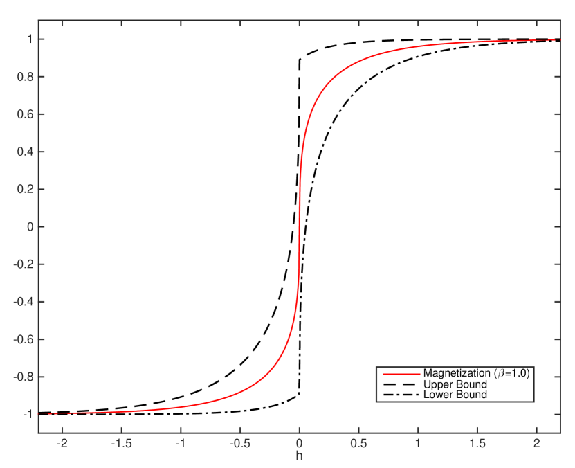
(a)

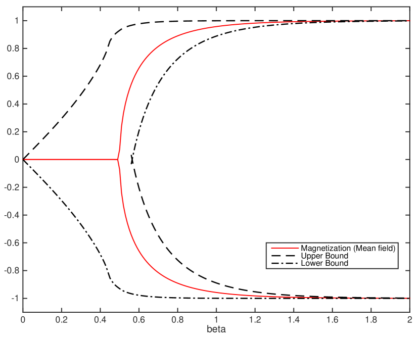
(b)

Figure 1: 1(a) The red solid line is the magnetization of 1-d mean field with $\beta=1$, which is the baseline; The black dashed/dash-dot lines is the goal-oriented divergence upper/lower bound of magnetization of the mean field with $\beta=1.6$. 1(b) The red solid line is the spontaneous magnetization of 2-d mean field Ising model for $\beta=1$, which is the baseline; The black dashed/dash-dot lines is the goal-oriented divergence upper/lower bound of the magnetization of the nearest neighbor Ising model with $\beta=1.6$.

This paper is organized as follows. In Section 2 we discuss classical information inequalities for QoIs and demonstrate that they do not scale with system size or with long time dynamics. We show these results by considering counterexamples such as sequences of independent identically distributed random variables and Markov chains. In Section 3 we revisit the concept of goal oriented divergence introduced earlier in [33] and show that it provides scalable and discriminating information bounds for QoIs. In Section 4 we discuss how these results extend to path-space observables, e.g., ergodic averages, autocorrelations, etc, where the role of relative entropy is now played by the relative entropy rate (RER) and connect to nonlinear response calculations for stochastic dynamics in statistical mechanics. In Section 5 we show how these new information inequalities transfer to Gibbs measures, implying nonlinear response UQ bounds, and how they relate to classical results for thermodynamic limits in statistical mechanics. Finally in Section 6 we apply our methods and the scalability of the UQ bounds to assess model and parametric uncertainty of phase diagrams in molecular systems. We demonstrate the methods for Ising models, although the perspective is generally applicable.

2 Poor scaling properties of the classical inequalities for probability metrics

In this section we discuss several classical information inequalities and demonstrate they scale poorly with the size of the system especially when applying the inequalities to ergodic averages. We make these points by considering simple examples such as independent, identically distributed (IID) random variables, as well as Markov sequences and the corresponding statistical estimators.

Suppose $P$ and $Q$ be two probability measures on some measure space $(\mathcal{X},\mathcal{A})$ and let $f:\mathcal{X}\to\mathbb{R}$ be some quantity of interest (QoI). Our goal is to consider the discrepancy between models $P$ and $Q$ with respect to the quantity of interest $f$,

$$E_{Q}(f)-E_{P}(f)\,.$$ (12)

Our primary mathematical challenge here is to understand what results on information metrics between probability measures $P$ and $Q$ imply for quantities of interest in (12). We first discuss several concepts of information metrics, including divergences and probability distances.

2.1 Information distances and divergences

To keep the notation as simple as possible we will assume henceforth that $P$ and $Q$ are mutually absolutely continuous and this will cover all the examples considered here. (Much of what we discuss would extend to general measures by considering a measure dominating $P$ and $Q$, e.g. $\frac{1}{2}(P+Q)$. For the same reasons of simplicity in presentation, we assume that all integrals below exist and are finite.

Total Variation [2]: The total variation distance between $P$ and $Q$ is defined by

$$TV(Q,P)=\sup_{A\in\mathcal{A}}\left|Q(A)-P(A)\right|=\frac{1}{2}\int\left|1-\frac{dP}{dQ}\right|dQ.$$ (13)

Bounds on $TV(Q,P)$ provide bounds on $|E_{Q}(f)-E_{P}(f)|$ since we have

$$TV(Q,P)\,=\,\frac{1}{2}\sup_{\|f\|_{\infty}=1}\left|E_{Q}(f)-E_{P}(f)\right|.$$ (14)

Relative entropy [2]: The Kullback-Leibler divergence, or relative entropy, of $P$ with respect to $Q$ is defined by

$$R(Q\mid\mid P)=\int\log\left(\frac{dQ}{dP}\right)dQ.$$ (15)

Relative R$\acute{e}$nyi entropy [37]: For $\alpha>0$, $\alpha\not=1$, the relative R$\acute{e}$nyi entropy (or divergence) of order $\alpha$ of $P$ with respect to $Q$ is defined by

$$D_{\alpha}(Q\mid\mid P)=\frac{1}{\alpha-1}\int\left(\frac{dP}{dQ}\right)^{1-\alpha}dQ=\frac{1}{\alpha-1}\int\left(\frac{dQ}{dP}\right)^{\alpha}dP.$$ (16)

$\chi^{2}$ divergence [2]: The $\chi^{2}$ divergence between $P$ and $Q$ is defined by:

$$\chi^{2}(Q\mid\mid P)=\int\left(\frac{dQ}{dP}-1\right)^{2}dP$$ (17)

Hellinger distance [2]: The Hellinger distance between $P$ and $Q$ is defined by:

$$H(Q,P)=\left(\int\left(1-\sqrt{\frac{dP}{dQ}}\right)^{2}dQ\right)^{1/2}$$ (18)

The total variation and Hellinger distances define proper distances while all the other quantities are merely divergences (i.e., they are non-negative and vanish if and only if $P=Q$). The R$\acute{e}$nyi divergence of order $1/2$ is symmetric in $P$ and $Q$ and is related to the Hellinger distance by

$$D_{1/2}(Q\mid\mid P)=-2\log\left(1-\frac{1}{2}H^{2}(Q,P)\right)\,.$$

Similarly the R$\acute{e}$nyi divergence of order $2$ is related to the $\chi^{2}$ divergence by

$$D_{2}(Q\mid\mid P)=\log\left(1+\chi^{2}(Q\mid\mid P)\right)\,.$$

In addition the R$\acute{e}$nyi divergence of order $\alpha$ is an nondecreasing function $\alpha$ [38] and we have

$$\lim_{\alpha\to 1}D_{\alpha}(Q\mid\mid P)=R(Q\mid\mid P).$$

and thus it thus natural to set $D_{1}(Q\mid\mid P)=R(Q\mid\mid P)$. Using the inequality $\log(t)\leq t-1$ we then obtain the chain of inequalities, [2]

$$H^{2}(Q,P)\leq D_{1/2}(Q\mid\mid P)\leq R(Q\mid\mid P)\leq D_{2}(Q\mid\mid P)\leq\chi^{2}(Q\mid\mid P)\,.$$ (19)

2.2 Some classical information inequalities for QoIs

We recall a number of classical information-theoretic bounds which use probability distances ot divergences to control expected values of QoIs (also referred to as observables). Because

$$|E_{Q}(f)-E_{P}(f)|\leq 2\|f\|_{\infty}TV(Q,P)$$

we can readily obtain bounds on QoIs from relationships between $TV(Q,P)$ and other divergences. It is well-known and easy to prove that $TV(Q,P)\leq H(Q,P)$ but we will use here the slightly sharper bound (Le Cam’s inequality) [2] given by

$$TV(Q,P)\leq H(Q,P)\sqrt{1-\frac{1}{4}H^{2}(Q,P)}$$

which implies

Le Cam[2]:

$$\left|E_{Q}(f)-E_{P}(f)\right|\leq 2\|f\|_{\infty}H(Q,P)\sqrt{1-\frac{1}{4}H^{2}(Q,P)}.$$ (20)

From inequality (19) and $TV(Q,P)\leq H(Q,P)$ we obtain immediately bounds on $TV(Q,P)$ by $\sqrt{D_{\alpha}(Q\mid\mid P)}$ but the constants are not optimal. The following generalized Pinsker inequality (with optimal constants) was proved in [39] and holds for $0<\alpha\leq 1$

$$TV(Q,P)\leq\sqrt{\frac{1}{2\alpha}D_{\alpha}(Q\mid\mid P)},$$

and leads to

Csiszar-Kullback-Pinsker (CKP) [2]:

$$\left|E_{Q}(f)-E_{P}(f)\right|\leq\|f\|_{\infty}\sqrt{2R(Q\mid\mid P)}.$$ (21)

Generalized Pinsker: see [38]: For $0<\alpha\leq 1$

$$\left|E_{Q}(f)-E_{P}(f)\right|\leq\|f\|_{\infty}\sqrt{\frac{2}{\alpha}D_{\alpha}(Q\mid\mid P)}.$$ (22)

It is known that the CKP inequality is sharp only of $P$ and $Q$ are close. In particular the total variation norm is always less than $1$ while the relative entropy can be very large. There is a complementary bound to the CKP inequality which is based on a result by Scheffé [2]

Scheffé:

$$\mid E_{Q}(f)-E_{P}(f)\mid\leq\|f\|_{\infty}\left(2-e^{-R(Q\mid\mid P)}\right).$$ (23)

By (19) we have $R(P\mid\mid Q)\leq\chi^{2}(Q\mid\mid P)$ and thus we can also obtain a bound in terms of the $\chi^{2}$ divergence and $\|f\|_{\infty}$. However, we can obtain a better bound which involves the variance of $f$ by using Cauchy-Schwartz inequality.

Chapman-Robbins [40]:

$$\left|E_{Q}(f)-E_{P}(f)\right|\leq\sqrt{Var_{P}(f)}\sqrt{\chi^{2}(Q\mid\mid P)}.$$ (24)

Hellinger-based inequalities:

Recently a bound using the Hellinger distance and the $L^{2}$ norm was derived in [41]:

$$\left|E_{Q}(f)-E_{P}(f)\right| \leq \sqrt{2}H(Q,P)\sqrt{(E_{P}(f^{2})+E_{Q}(f^{2}))}.$$

As we show in Section A this bound can be further optimized by using a control variates argument. Note that the left hand side is unchanged by replacing $f$ by $f-\frac{1}{2}(E_{P}(f)+E_{Q}(f))$ and this yields the improved bound

$$\left|E_{Q}(f)-E_{P}(f)\right| \leq \sqrt{2}H(Q,P)\sqrt{Var_{P}(f)+Var_{P}(f)+\frac{1}{2}(E_{Q}(f)-E_{P}(f))^{2}}.$$ (25)

2.3 Scaling properties for IID sequences

We make here some simple, yet useful observations, on how the inequalities discussed in the previous Section scale with system size for IID sequences. We consider the product measure space $\mathcal{X}_{N}=\mathcal{X}\times\cdots\times\mathcal{X}$ equipped with the product $\sigma$-algebra $\mathcal{A}_{N}$ and we denote by $P_{N}=P\times\cdots\times P$ the product measures on $(\mathcal{X}_{N},\mathcal{A}_{N})$ whose all marginals are equal to $P$ and we define $Q_{N}$ similarly. From a statistics perspective, this is also the setting where sequences of $N$ independent samples are generated by the models $P$ and $Q$ respectively.

We will concentrate on QoIs which are observables which have the form of ergodic averages or of statistical estimators. The challenge would be to assess based on information inequalities the impact on the QoIs. Next, we consider the simplest such case of the sample mean. For any measurable $g:\mathcal{X}\to\mathbb{R}$ we consider the observable $f_{N}:\mathcal{X}_{N}\to\mathbb{R}$ given by

$$f_{N}(\sigma_{1},\cdots\sigma_{N})=\frac{1}{N}\sum_{j=1}^{N}g(\sigma_{j})\,,$$ (26)

This quantity is also the sample average of the data set ${\mathcal{D}}=\{\sigma_{1},\cdots\sigma_{N}\}$. We also note that

$$\|f_{N}\|_{\infty}=\|g\|_{\infty}\,,\quad\quad E_{P_{N}}(f_{N})=E_{P}(g)\,,\quad\quad\quad\quad Var_{P_{N}}(f_{N})=\frac{1}{N}Var_{P}(g)$$

To understand how the various inequalities scale with the system size $N$ we need to understand how the information distances and divergences themselves scale with $N$. For IID random variables the results are collected in the following Lemma.

Lemma 2.1.

For two product measures $P_{N}$ and $Q_{N}$ with marginals $P$ and $Q$ we have

Kullback-Leibler: $$R(Q_{N}\mid\mid P_{N})=NR(Q\mid\mid P)$$ (27)

Rényi : $$D_{\alpha}(Q_{N}\mid\mid P_{N})=ND_{\alpha}(Q\mid\mid P)$$

Chi-squared: $$\chi^{2}(Q_{N}\mid\mid P_{N})=\left(1+\chi^{2}(Q\mid\mid P)\right)^{N}-1$$

Hellinger: $$H(Q_{N}\mid\mid P_{N})=\sqrt{2-2\left(1-\frac{H^{2}(Q,P)}{2}\right)^{N}}$$

Proof.

See B.

Combining the result in Lemma 2.1 with the information bounds in the previous Section we obtain a series of bounds for ergodic averages which all suffer from serious defects. Some grow to infinity for $N\gg 1$ while others converge to a trivial bound that is not discriminating, namely provide no new information on the difference of the QoIs $E_{Q_{N}}(f_{N})-E_{P_{N}}(f_{N})$. More precisely we obtain the following bounds:

Csiszar-Kullback-Pinsker (CKP) for IID:

$$\left|E_{Q_{N}}(f_{N})-E_{P_{N}}(f_{N})\right|\leq\|g\|_{\infty}\sqrt{2NR(Q\mid\mid P)}=O(\sqrt{N}).$$ (28)

Generalized Pinsker for IID: For $0<\alpha<1$ we have

$$\left|E_{Q_{N}}(f_{N})-E_{P_{N}}(f_{N})\right|\leq\|g\|_{\infty}\sqrt{\frac{2N}{\alpha}D_{\alpha}(Q\mid\mid P)}=O(\sqrt{N}).$$ (29)

Scheffé for IID:

$$\left|E_{Q_{N}}(f_{N})-E_{P_{N}}(f_{N})\right|\leq\|g\|_{\infty}\left(2-e^{-NR(Q\mid\mid P)}\right)=O(1).$$ (30)

Chapman-Robbins for IID: We have

$$\left|E_{Q_{N}}(f_{N})-E_{P_{N}}(f_{N})\right|\leq\sqrt{\frac{1}{N}Var_{P}(g)}\sqrt{\left(1+\chi^{2}(Q\mid\mid P)\right)^{N}-1}=O\left(\frac{{\sqrt{e^{N}}}}{\sqrt{N}}\right).$$ (31)

Le Cam for IID:

$$\left|E_{Q_{N}}(f_{N})-E_{P_{N}}(f_{N})\right| \leq 2\|g\|_{\infty}\sqrt{2-2\left(1-\frac{H^{2}(Q,P)}{2}\right)^{N}}\sqrt{\frac{1}{2}+\frac{1}{2}\left(1-\frac{H^{2}(Q,P)}{2}\right)^{N}}$$ (32)

$$= O(1).$$

Hellinger for IID:

$$\left|E_{Q_{N}}(f_{N})-E_{P_{N}}(f_{N})\right| \leq \sqrt{2}\sqrt{2-2\left(1-\frac{H^{2}(Q,P)}{2}\right)^{N}}\sqrt{\frac{Var_{P}(g)}{N}+\frac{Var_{Q}(g)}{N}+\frac{1}{2}(E_{P}(g)-E_{Q}(g))^{2}}.$$ (33)

Every single bound fails to capture the behavior of ergodic averages. Note that the left-hand sides are all of order $1$ and indeed should be small of $P$ and $Q$ are sufficiently close to each other. The CKP, generalized Pinsker and Chapman-Robbins bounds all diverge as $N\to\infty$ and thus completely fail. The Le Cam bound is of order $1$, but as $N\to\infty$ the bound converges to $2\|f\|_{\infty}$ which is a trivial bound independent of $P$ and $Q$. The Scheffé likewise converges to constant. Finally the Dashti-Stuart bound converges to the trivial statement that $1\leq\sqrt{2}$.

2.4 Scaling properties for Markov sequences

Next, we consider the same questions as in the previous Section, however this time for correlated distributions. Let two Markov chains in a finite state space $S$ with transitions matrix $p(x,y)$ and $q(x,y)$ respectively. We will assume that both Markov chains are irreducible with stationary distributions $\mu_{p}$ and $\mu_{q}$ respectively. In addition we assume that for any $x\in S$, the probability measure $p(x,\cdot)$ and $q(x,\cdot)$ are mutually absolutely continuous. We denote by $\nu_{p}(x)$ and $\nu_{q}(x)$ the initial distributions of the two Markov chains and then the probability distributions of the path $(X_{1},\cdots X_{N})$ evolving under $p$ is given by

$$P_{N}(X_{1},\cdots,X_{N})=\nu_{p}(X_{0})p(X_{0},X_{1})\cdots p(X_{N-1},X_{N})\,,$$

and similarly for the distribution $Q_{N}$ under $q$.

If we are interested in the long-time behavior of the system, for example we may be interested in computing or estimating expectations of the steady state or in our case model discrepancies such as

$$\left|E_{\mu_{q}}(g)-E_{\mu_{p}}(g)\right|$$

for some QoI (observable) $g:S\to\mathbb{R}$. In general the steady state of a Markov chain is not known explicitly or it is difficult to compute for large systems. However, if we consider ergodic observables such as

$$f_{N}(X_{1},\cdots X_{N})=\frac{1}{N}\sum_{i=1}^{N}g(X_{i})$$ (34)

then, by the ergodic theorem, we have, for any initial distribution $\nu_{p}(x)$ that

$$\lim_{N\to\infty}E_{P_{N}}(f_{N})=E_{\mu_{p}}(g)\,.$$

and thus can estimate $|E_{\mu_{q}}(g)-E_{\mu_{p}}(g)|$ if we can control $|E_{Q_{N}}(f)-E_{P_{N}}(f)|$ for large $N$. After our computations with IID sequences in the previous Section, it is not surprising that none of the standard information inequalities allow such control. Indeed the following lemma, along with the fact that the variance of ergodic observables such as (34) scales like $Var_{P_{N}}(f_{N})=O(1/N)$ [33], readily imply that the bounds for Markov measures scale exactly as (poorly as) the IID case, derived at the end of Section 2.3.

Lemma 2.2.

Consider two irreducible Markov chains with transitions matrix $p$ and $q$. Assume that the initial conditions $\nu_{p}(x)$ and $\nu_{q}(x)$ are mutually absolutely continuous and that $p(x,\cdot)$ and $q(x,\cdot)$ are mutually absolutely continuous for each $x$.

Kullback-Leibler: We have

$$\lim_{N\to\infty}\frac{1}{N}R(Q_{N}\mid\mid P_{N})=r(q\mid\mid p):=\sum_{x,y}\mu_{q}(x)q(x,y)\log\left(\frac{q(x,y)}{p(x,y)}\right)\,,$$

and the limit is positive if and only if $p\not=q$.

Rényi : We have

$$\lim_{N\to\infty}\frac{1}{N}D_{\alpha}(Q_{N}\mid\mid P_{N})=\frac{1}{\alpha-1}\log\rho(\alpha)\,,$$

where $\rho(\alpha)$ is the maximal eigenvalue of the non-negative matrix with entries $q^{\alpha}(x,y)p^{1-\alpha}(x,y)$ and we have $\frac{1}{\alpha-1}\log\rho(\alpha)\geq 0$ with equality if and only if $p\not=q$.

Chi-squared: We have

$$\lim_{N\to\infty}\frac{1}{N}\log(1+\chi^{2}(Q_{N}\mid\mid P_{N}))=\log\rho(2)$$

where $\rho(2)$ is the maximal eigenvalue of the matrix with entries $q^{2}(x,y)p^{-1}(x,y)$ and we have $\log\rho(2)\geq 0$ with equality if and only if $p=q$.

Hellinger: We have

$$\lim_{N\to\infty}H(Q_{N}\mid\mid P_{N})=\sqrt{2}.$$

if $p\not=q$ and $0$ if $p=q$.

Proof.

See Appendix B.

3 A divergence with good scaling properties

3.1 Goal Oriented Divergence

In this Section we will first discuss the goal-oriented divergence which was introduced by [33], following the work in [34]. Subsequently in Sections 3.3 and 4 and Section 5 we will demonstrate that this new divergence provides bounds on the model discrepancy $E_{Q}(f)-E_{P}(f)$ between models $P$ and $Q$ which scale correctly with their system size, provided the QoI $f$ has the form of an ergodic average or a statistical estimator.

Given an observable $f:\mathcal{X}\to\mathbb{R}$ we introduce the cumulant generating function of $f$

$$\Lambda_{P,f}(c)=\log E_{P}(e^{cf}).$$ (35)

We will assume $f$ is such that $\Lambda_{P,f}(c)$ is finite in a neighborhood $(-c_{0},c_{0})$ of the origin. For example if $f$ is bounded then we can take $c_{0}=\infty$. Under this assumption $f$ has finite moments of any order and we will often use the cumulant generating function of a mean $0$ observable

$$\widetilde{\Lambda}_{P,f}(c)=\log E_{P}(e^{c(f-E_{P}(f))})=\Lambda_{P,f}(c)-cE_{P}(f).$$ (36)

The following bound is proved in [33] and will play a fundamental role in the rest of the paper.

Goal-oriented divergence UQ bound: If $Q$ is absolutely continuous with respect to $P$ and ${\Lambda}_{P,f}(c)$ is finite in a neighborhood of the origin, then

$$\Xi_{-}(Q\mid\mid P;f)\leq E_{Q}(f)-E_{P}(f)\leq\Xi_{+}(Q\mid\mid P;f).$$ (37)

where

$$\Xi_{+}(Q\mid\mid P;f) = \inf_{c>0}\left\{\frac{1}{c}\widetilde{\Lambda}_{P,f}(c)+\frac{1}{c}R(Q\mid\mid P)\right\}$$ (38)

$$\Xi_{-}(Q\mid\mid P;f) = \sup_{c>0}\left\{-\frac{1}{c}\widetilde{\Lambda}_{P,f}(-c)-\frac{1}{c}R(Q\mid\mid P)\right\}.$$ (39)

We refer to [33] and [34] for details of the proof but the main idea behind the proof is the variational principle for the relative entropy: for bounded $f$ we have, [42],

$$\log E_{P}(e^{f})=\sup_{Q}\left\{E_{Q}(f)-R(Q\mid\mid P)\right\}$$

and thus for any $Q$

$$E_{Q}(f)\leq\log E_{P}(e^{f})+R(Q\mid\mid P)\,.$$

Replacing $f$ by $c(f-E_{P}(f))$ with $c>0$ and optimizing over $c$ yields the upper bound. The lower bound is derived in a similar manner.

Robustness: These new information bounds were shown in [34] to be robust in the sense that the upper bound is attained when considering all models $Q$ with a specified uncertainty threshold given by $R(Q\mid\mid P)\leq\eta$. Furthermore, the parameter $c$ in the variational representations (38) and (39) controls the degree of robustness with respect to the model uncertainty captured by $R(Q\mid\mid P)$. In a control or optimization context these bounds are also related to H^∞ control, [36].

As the following result from [33] shows, the quantities $\Xi_{+}$ and $\Xi_{-}$ are divergences similar to the relative (R$\acute{e}$nyi ) entropy, the $\chi^{2}$ divergence and the Hellinger distance. Yet they depend on the observable $f$ and thus will be referred to as goal-oriented divergences.

Properties of the goal-oriented divergence:

1. $\Xi_{+}(Q\mid\mid P;f)\geq 0$ and $\Xi_{-}(Q\mid\mid P;f)\leq 0$.

2. $\Xi_{\pm}(Q\mid\mid P;f)=0$ if and only if $Q=P$ or $f$ is constant P-a.s.

It is instructive to understand the bound when $P$ and $Q$ are close to each other. Again we refer to [33] for a proof and provide here just an heuristic argument. First note that if $P=Q$ then it is easy to see that the infimum in the upper bound is attained at $c=0$ since $R(Q\mid\mid P)=0$ and $\widetilde{\Lambda}_{P,f}(c)>0$ for $c>0$ (the function is convex in $c$ and we have $\widetilde{\Lambda}_{P,f}(0)=\widetilde{\Lambda}_{P,f}^{\prime}(0)=0$ and $\widetilde{\Lambda}_{P,f}^{\prime\prime}(0)=\frac{1}{2}Var_{P}(f)$. So if $R(Q\mid\mid P)$ is small, we can expand the right-hand side in $c$ and we need to find

$$\inf_{c>0}\left\{c\frac{Var_{P}(f)}{2}+O(c^{2})+\frac{1}{c}R(Q\mid\mid P)\right\}\,.$$

Indeed, we find that the minimum has the form $\sqrt{Var_{P}(f)}\sqrt{2R(Q\mid\mid P)}+O(R(Q\mid\mid P))$, [33]. The lower bound is similar and we obtain:

Linearized UQ bound [33]: If $R(P\mid\mid Q)$ is small we have

$$\mid E_{Q}(f)-E_{P}(f)\mid\leq\sqrt{Var_{P}(f)}\sqrt{2R(Q\mid\mid P)}+O(R(Q\mid\mid P)).$$ (40)

3.2 Example: Exponential Family

Next we compute the goal-oriented divergences for an exponential family which covers many cases of interest including Markov and Gibbs measures (see Sections 3.4 and 4), as well as numerous probabilistic models in machine learning [4, 3].

Given a reference measure $P^{0}$ (which does not need to be a finite measure) we say that $P^{\theta}$ is an exponential family if $P^{\theta}$ is absolutely continuous with respect to $P^{0}$ with

$$\frac{dP^{\theta}}{dP^{0}}(x)=\exp\left(t(x)\cdot\theta-F(\theta)\right)$$

where $\theta=[\theta_{1},\cdots,\theta_{K}]^{T}\in\Theta\subset\mathbb{R}^{K}$ is the parameter vector, $t(x)=[t_{1}(x),...,t_{K}(x)]^{T}$ is the sufficient statistics vector and $F(\theta)$ is the log-normalizer

$$F(\theta)=\log\int e^{t(x)\cdot\theta}dP^{0}(x)\,.$$

Note that $F(\theta)$ is a cumulant generating function for the sufficient statistics, for example we have $\nabla_{\theta}F(\theta)=E_{P^{\theta}}(t)$. The relative entropy between two members of the exponential family is then computed as

$$R(P^{\theta^{\prime}}\mid\mid P^{\theta})=\int\log\frac{dP^{\theta^{\prime}}}{dP^{\theta}}(x)dP^{\theta^{\prime}}(x) = E_{P^{\theta^{\prime}}}\left((\theta^{\prime}-\theta)\cdot t(x)\right)+F(\theta)-F(\theta^{\prime})$$ (41)

$$= (\theta^{\prime}-\theta)\cdot\nabla F(\theta^{\prime})+F(\theta)-F(\theta^{\prime})$$

If we consider an observable which is a linear function of the sufficient statistics, that is

$$f(x)=t(x)\cdot v$$ (42)

for some vector $v\in\mathbb{R}^{K}$ then the cumulant generating function of $f-E_{P^{\theta}}(f)$ is

$$\tilde{\Lambda}_{P^{\theta},f}(c)=\log E_{P^{\theta}}[e^{cf}]-cE_{P^{\theta}}(f)=F(\theta+cv)-F(\theta)-cv\cdot\nabla F(\theta).$$ (43)

and thus combining (41) and (43), we obtain the divergences

$$\Xi_{+}(P^{\theta^{\prime}}\|P^{\theta};f) = \inf_{c>0}\frac{1}{c}\{(\theta^{\prime}-\theta)\cdot\triangledown F(\theta^{\prime})-F(\theta^{\prime})+F(\theta+cv)-cv\cdot\triangledown F(\theta)\}$$ (44)

$$\Xi_{-}(P^{\theta^{\prime}}\|P^{\theta};f) = \sup_{c>0}(-\frac{1}{c})\{(\theta^{\prime}-\theta)\cdot\triangledown F(\theta^{\prime})-F(\theta^{\prime})+F(\theta-cv)+cv\cdot\triangledown F(\theta)\}$$ (45)

Note that if our observable is not in the sufficient statistics class then we can obtain a similar formula by simply enlarging the sufficient statistics to include the observable in question.

3.3 Example: IID sequences

To illustrate the scaling properties of the goal-oriented divergence consider first two product measures $P_{N}$ and $Q_{N}$ as in Section 2.3 and the same sample mean observable (26). We now apply the bounds (38) and (39) to $Nf_{N}=\sum_{k=1}^{N}g(\sigma_{k})$ to obtain

$$\frac{1}{N}\Xi_{-}(Q_{N}\mid\mid P_{N};Nf_{N})\leq E_{Q_{N}}(f_{N})-E_{P_{N}}(f_{N})\leq\frac{1}{N}\Xi_{+}(Q_{N}\mid\mid P_{N};Nf_{N}).$$

The following lemma shows that the bounds scale correctly with $N$.

Lemma 3.1.

We have

$$\Xi_{\pm}(Q_{N}\mid\mid P_{N};Nf_{N})=N\Xi_{\pm}(Q\mid\mid P;g)\,.$$

Proof.

We have already noted that $R(Q_{N}\mid\mid P_{N})=NR(Q\mid\mid P)$. Furthermore

$${\widetilde{\Lambda}}_{P_{N},Nf_{N}}(c) = \log E_{P_{N}}(e^{cNF_{N}})-cE_{P_{N}}(Nf_{N})$$ (46)

$$= \log\int_{\mathcal{X}_{N}}e^{c\sum_{i=1}^{N}g(\sigma_{i})}\prod_{i=1}^{N}dP(\sigma_{i})-cE_{P_{N}}\left(\sum_{i=1}^{N}g(\sigma_{i})\right)$$

$$= N\log E_{P}(e^{cg})-cNE_{P}(g)=N{\widetilde{\Lambda}}_{P,g}(c).$$

This result shows that the goal oriented divergence bounds captures perfectly the behavior of ergodic average as $N$ goes to infinity. In particular when P and Q are very close, $\Xi_{\pm}(Q\mid\mid P;g)\to 0$, which contrasts sharply with all the bounds in Section 2.3.

4 UQ and nonlinear response bounds for Markov sequences

In the context of Markov chains, there are a number of UQ challenges which are usually not addressed by standard numerical analysis or UQ techniques: (a) Understand the effects of a model uncertainty on the long-time behavior (e.g. steady state) of the model. (b) Go beyond linear response and be able to understand how large perturbations affect the model, both in finite and long time regimes. (c) Have a flexible framework allowing to compare different models as, for example for Ising model versus mean-field model approximations considered in Section 6.

The inequalities of Section 3.1 can provide new insights to all three questions, at least when the bounds can be estimated or computed numerically or analytically. As a first example in this direction we consider Markov dynamics with the same set-up as in Section 2.4. We have the following bounds which exemplify how the goal-oriented divergences provide UQ bounds for the long-time behavior of Markov chains.

Theorem 4.1.

Consider two irreducible Markov chains with transition matrices $p(x,y)$ and $q(x,y)$ and stationary distributions $\mu_{p}$ and $\mu_{q}$ respectively. If $p(x,\cdot)$ and $q(x,\cdot)$ are mutually absolutely continuous we have for any observable $g$ the bounds

$$\xi_{-}(q\mid\mid p;g)\leq E_{\mu_{q}}(g)-E_{\mu_{p}}(g)\leq\xi_{+}(q\mid\mid p;g)\,,$$

where

$$\xi_{+}(q\mid\mid p;g) = \inf_{c\geq 0}\left\{\frac{1}{c}\lambda_{p,g}(c)+\frac{1}{c}r(q\mid\mid p)\right\}$$

$$\xi_{-}(q\mid\mid p;g) = \sup_{c\geq 0}\left\{-\frac{1}{c}\lambda_{p,g}(-c)-\frac{1}{c}r(q\mid\mid p)\right\}\,.$$ (47)

Here

$$r(q\mid\mid p)=\lim_{N\to\infty}\frac{1}{N}R(Q_{N}\mid\mid P_{N})$$

is the relative entropy rate and $\lambda_{p,g}(c)$ is the logarithm of the maximal eigenvalue of the non-negative matrix with entries $p(x,y)\exp(c(g(y)-E_{\mu_{p}}(g)))$.

Moreover, we have the asymptotic expansion in relative entropy rate $r(q\mid\mid p)$,

$$\left|E_{\mu_{q}}(g)-E_{\mu_{p}}(g)\right|\leq\sqrt{v_{\mu_{p}}(g)}\sqrt{2r(q\mid\mid p)}+O(r(q\mid\mid p))$$ (48)

where

$$v_{\mu_{p}(g)}\,=\,\sum_{k=-\infty}^{\infty}E_{\mu_{p}}\left(g(X_{k})g(X_{0})\right)$$

is the integrated auto-correlation function for the observable $g$.

Proof.

We apply the goal-oriented divergence bound to the observable $Nf_{N}=\sum_{k=1}^{N}g(X_{i})$ and have

$$\frac{1}{N}\Xi_{-}(Q_{N}\mid\mid P_{N};Nf_{N})\leq E_{Q_{N}}(f_{N})-E_{P_{N}}(f_{N})\leq\frac{1}{N}\Xi_{+}(Q_{N}\mid\mid P_{N};Nf_{N}).$$

We then take the limit $N\to\infty$. By the ergodicity of $P_{N}$ we have $\lim_{N\to\infty}E_{P_{N}}(f_{N})=E_{\mu_{p}}(g)$ and similarly for $Q_{N}$. We have already established in Lemma 2.2 the existence of the limit $r(q\mid\mid p)\,=\,\lim_{N\to\infty}\frac{1}{N}R(Q_{N}\mid\mid P_{N})$. For the moment generating function in $\Xi_{\pm}$ we have

$$\frac{1}{N}\widetilde{\Lambda}_{P_{N},Nf_{N}}(c) = \frac{1}{N}\log E_{P_{N}}(e^{cNf_{N}})-c\frac{1}{N}E_{P_{N}}(Nf_{N})$$

$$= \frac{1}{N}\log\sum_{X_{0},\cdots X_{N}}\nu_{p}(X_{0})\prod_{k=1}^{N}p(X_{k-1},X_{k})e^{cg(X_{k})}-cE_{P_{N}}(f_{N})$$

$$= \frac{1}{N}\log\nu_{p}P_{cg}^{N}-cE_{P_{N}}(f_{N})$$

where $P_{cg}$ is the non-negative matrix with entries $p(x,y)e^{cg(y)}$. The Perron-Frobenius theorem gives the existence of the limit.

The asymptotic expansion is proved exactly as for the linearized UQ bound (40). It is not difficult to compute the second derivative of $\frac{1}{c}\lambda_{p,g}(c)$ with respect to $c$ by noting all function are analytic of function of $c$ and thus we can freely exchange the $N\to\infty$ limit with the derivative with respect to $c$. Therefore we obtain that

$$\frac{d^{2}}{dc^{2}}\lambda_{P,g}(0)\,=\,\lim_{N\to\infty}Var_{P_{N}}(Nf_{N})$$

and a standard computation shows that the limit is the integrated autocorrelation function $v_{\mu_{p}}(g)$.

Remark: A well studied case of UQ for stochastic models and in particular stochastic dynamics is linear response, also referred to as local sensitivity analysis, which addresses the role of infinitesimal perturbations to model parameters of probabilistic models, e.g. [43, 44]. Here (48) provides computable bounds in the linear response regime, as demonstrated earlier in [33] and which can be used for fast screening of uninfluential parameters in reaction networks with a very large number of parameters, [45].

Nonlinear response bounds: Beyond linear response considerations, nonlinear response methods attempt to address the role of larger parameter perturbations. Some of the relevant methods involve asymptotic series expansions in terms of the small parameter perturbation [46, 47], which quickly become computationally intractable as more terms need to be computed. However, the inequalities (38) and (39) provide robust and computable nonlinear response bounds.

The main result in Theorem 4.1 was first obtained in [33]. Here we revisit it in the context of scalability in both space and time and connect it to nonlinear response calculations for stochastic dynamics in statistical mechanics. This connection is made more precise in the following Corollaries which follow from Theorem 4.1 and provide layers of progressively simpler-and accordingly less sharp-bounds:

Corollary 4.2.

Based on the assumptions and definitions in Theorem 4.1, we have the following two bounds that involve two upper bounds of $r(q\mid\mid p)$. Bound (i) is sharper than bound (ii), while the latter is straightforward to calculate analytically.

(i) Let $R(q(x,\cdot)\|p(x,\cdot))=\sum_{y}q(x,y)\log\frac{q(x,y)}{p(x,y)}$; then,

$$\xi_{+}(q\mid\mid p;g) \leq \inf_{c\geq 0}\left\{\frac{1}{c}\lambda_{p,g}(c)+\frac{1}{c}\sup_{x}R(q(x,\cdot)\|p(x,\cdot))\right\}$$

$$\xi_{-}(q\mid\mid p;g) \geq \sup_{c\geq 0}\left\{-\frac{1}{c}\lambda_{p,g}(-c)-\frac{1}{c}\sup_{x}R(q(x,\cdot)\|p(x,\cdot))\right\}\,.$$ (49)

(ii) Next, we have the upper bound in terms of the quantity $\sup\limits_{x,y}|\log\frac{q(x,y)}{p(x,y)}|$,

$$\xi_{+}(q\mid\mid p;g) \leq \inf_{c\geq 0}\left\{\frac{1}{c}\lambda_{p,g}(c)+\frac{1}{c}\sup_{x,y}|\log\frac{q(x,y)}{p(x,y)}|\right\}$$

$$\xi_{-}(q\mid\mid p;g) \geq \sup_{c\geq 0}\left\{-\frac{1}{c}\lambda_{p,g}(-c)-\frac{1}{c}\sup_{x,y}|\log\frac{q(x,y)}{p(x,y)}|\right\}\,.$$ (50)

Proof.

We consider the relative entropy rate $r(q\mid\mid p)$,

$$r(q\mid\mid p) =\sum_{x,y}\mu_{q}(x)q(x,y)\log\frac{q(x,y)}{p(x,y)}$$

$$=E_{\mu_{q}(x)}\left(\sum_{y}q(x,y)\log\frac{q(x,y)}{p(x,y)}\right)$$

$$=E_{\mu_{q}(x)}\left(R(q(x,\cdot)\|p(x,\cdot))\right)$$

$$\leq\sup_{x}R(q(x,\cdot)\|p(x,\cdot)),$$ (51)

where $R(q(x,\cdot)\|p(x,\cdot))=\sum_{y}q(x,y)\log\frac{q(x,y)}{p(x,y)}$. Moreover, we have

$$R(q(x,\cdot)\|p(x,\cdot))=\sum_{y}q(x,y)\log\frac{q(x,y)}{p(x,y)}\leq\sup_{y}|\log\frac{q(x,y)}{p(x,y)}|.$$

Therefore we can obtain another bound for $r(q\mid\mid p)$, that is,

$$r(q\mid\mid p)\leq\sup_{x,y}|\log\frac{q(x,y)}{p(x,y)}|.$$ (52)

This bound may be not as sharp as the one in (4), but it is more easily computable. Thus, by (4.1), (4) and (52), it is easy to obtain (i) and (ii).

If we consider the linearized bound in (48), then combining the bounds (4) and (52) of $r(q\|p)$, we can obtain the following bound, which is a further simplification of Corollary 4.2, again at the expense of the tightness of the bounds.

Corollary 4.3.

Under the assumptions and definitions in Theorem 4.1, we have:

$$\xi_{\pm}(q\mid\mid p;g) \leq \pm\sqrt{v_{\mu_{p}}(g)}\sqrt{2\sup_{x}R(q(x,\cdot)\|p(x,\cdot))}+O(\sup_{x}R(q(x,\cdot)\|p(x,\cdot)))$$ (53)

$$\leq \pm\sqrt{v_{\mu_{p}}(g)}\sqrt{2\sup_{x,y}|\log\frac{q(x,y)}{p(x,y)}|}+O(\sup_{x,y}|\log\frac{q(x,y)}{p(x,y)}|).$$ (54)

Remark: By the previous two Corollaries, we get some cheap ways to replace the calculation of $\xi_{\pm}(q\mid\mid p;g)$ since it is much easier to calculate $\sup\limits_{x}R(q(x,\cdot)\|p(x,\cdot))$ or $\sup\limits_{x,y}|\log\frac{q(x,y)}{p(x,y)}|$ than $r(q\|p)$ itself, especially the latter one. In practice, we can first attempt to estimate $\xi_{\pm}(q\mid\mid p;g)$ by calculating the leading term in (53) or (54). If the the linearization assumptions in the last Corollary fail, then we can try to use Corollary 4.2 or Theorem 4.1 which can also give computable bounds or estimates of $\xi_{\pm}(q\mid\mid p;g)$.

Finally, the bound in (52) is the Markov chain analogue of the triple norm $|||\cdot|||$ used in the estimation of UQ bounds for QoIs of Gibbs measures, which we discuss in depth in Section 5.

5 UQ and nonlinear response bounds for Gibbs measures

The Gibbs measure is one of the central objects in statistical mechanics and molecular dynamics simulation, [32], [48]. On the other hand Gibbs measures in the form of Boltzmann Machines or Markov Random Fields provide one of the key classes of models in machine learning and pattern recognition, [3, 4]. Gibbs measures are probabilistic models which are inherently high dimensional, describing spatially distributed systems or a large number of interacting molecules. In this Section we derive scalable UQ bounds for Gibbs measures based on the goal oriented inequalities discussed in Section 3.1. Gibbs measures can be set on a lattice or in continuum space, here for simplicity in the presentation we focus on lattice systems.

Lattice spins systems. We consider Gibbs measures for lattice systems on $\mathbb{Z}^{d}$. If we let $S$ be the configuration space of a single particle at a single site $x\in\mathbb{Z}^{d}$, then $S^{X}$ is the configuration space for the particles in $X\subset\mathbb{Z}^{d}$; we denote by $\sigma_{X}\,=\,\{\sigma_{x}\}_{x\in X}$ an element of $S^{X}$. We will be interested in large systems so we let $\Lambda_{N}=\{x\in\mathbb{Z}^{d},|x_{i}|\leq n\}$ denote the square lattice with $N=(2n+1)^{d}$ lattice sites. We shall use the shorthand notation $\lim\limits_{N}$ to denote taking limit along the increasing sequence of lattices $\Lambda_{N}$ which eventually cover $\mathbb{Z}^{d}$.

Hamiltonians, interactions, and Gibbs measures. To specify a Gibbs measures we specify the energy $H_{N}(\sigma_{\Lambda_{N}})$ of a set of particles in the region $\Lambda_{N}$. It is convenient to introduce the concept of an interaction $\Phi=\{\Phi_{X}:X\subset\mathbb{Z}^{d},X\textrm{finite}\}$ which associates to any finite subset $X$ a function $\Phi_{X}(\sigma_{X})$ which depends only on the configuration in $X$. We shall always assume that interactions are translation-invariant, that is for any $X\subset\mathbb{Z}^{d}$ and any $a\in\mathbb{Z}^{d}$, $\Phi_{X+a}$ is obtained by translating $\Phi_{X}$. For translation-invariant interactions we have the norm [32]

$$|||\Phi|||=\sum_{\mathrm{X}\ni 0}|\mathrm{X}|^{-1}\|\Phi_{X}\|_{\infty}$$ (55)

and denote by $\mathcal{B}$ the corresponding Banach space of interactions. Given an interaction $\Phi$ we then define the Hamiltonians $H^{\Phi}_{N}$ (with free boundary conditions) by

$$H_{N}^{\Phi}(\sigma_{\Lambda_{N}})=\sum_{X\subset\Lambda_{N}}\Phi_{X}(\sigma_{X}),$$ (56)

and Gibbs measures $\mu_{N}^{\Phi}$ by

$$d\mu_{N}^{\Phi}(\sigma_{\Lambda_{N}})=\frac{1}{Z_{N}^{\Phi}}e^{-H_{N}(\sigma_{\Lambda_{N}})}dP_{N}(\sigma_{\Lambda_{N}}),$$ (57)

where $P_{N}$ is the counting measure on $S^{\Lambda_{N}}$ and $Z_{N}^{\Phi}=\sum_{\sigma_{\Lambda_{N}}}e^{-H_{N}(\sigma_{\Lambda_{N}})}$ is the normalization constant. In a similar way one can consider periodic boundary conditions or more general boundary conditions, see [32] for details.

Example: Ising model. For the $d$-dimensional nearest neighbor Ising model at inverse temperature $\beta$ we have

$$H_{N}(\sigma_{\Lambda_{N}})\,=\,-\beta J\sum_{\langle x,y\rangle\subset\Lambda_{N}}\sigma(x)\sigma(y)-\beta h\sum_{x\in\Lambda_{N}}\sigma(x)$$

where $\langle x,y\rangle$ denotes a pair of neighbors with $\sup\limits_{i}|x_{i}-y_{i}|=1$. So we have

$$\Phi_{X}=\left\{\begin{array}[]{cc}-\beta J\sigma(x)\sigma(y)\,,&X=\{x,y\},\\ -\beta h\sigma(x)\,,&X=\{x\},\\ 0&\textrm{otherwise},\\ \end{array}\right.$$

and it is easy to see that (55) becomes

$$|||\Phi|||=\beta(d|J|+|h|).$$

Observables. We will consider observables of the form

$$f_{N}(\sigma_{\Lambda_{N}})=\frac{1}{N}\sum_{x\in\Lambda_{N}}g(\sigma_{x})$$

for some observable $g$. It will be useful to note that $Nf_{N}$ is nothing but Hamiltonian $H_{N}^{\Gamma^{g}}$ for the interaction $\Gamma^{g}$ with

$$\Gamma^{g}_{\{x\}}=g\,,\quad\mbox{and}\quad\Gamma^{g}_{X}=0\quad\mbox{if}\quad X\not=\{x\}\,.$$ (58)

UQ bounds for Gibbs measures in finite volume. Given two Gibbs measure $\mu_{N}^{\Phi}$ and $\mu_{N}^{\Psi}$ straightforward computations show that for the relative entropy we have

$$R(\mu_{N}^{\Psi}\mid\mid\mu_{N}^{\Phi})\,=\,\log Z_{N}^{\Phi}-\log Z_{N}^{\Psi}+E_{\mu_{N}^{\Psi}}(H_{N}^{\Phi}-H_{N}^{\Psi})\,.$$ (59)

while for the cumulant generating function we have

$$\widetilde{\Lambda}_{\mu_{N}^{\Phi},Nf_{N}}(c)=\log Z_{N}^{\Phi-c\Gamma^{g}}-\log Z_{N}^{\phi}-cE_{\mu_{N}^{\Phi}}(Nf_{N})$$ (60)

and thus we obtain immediately from the results in Section 3.1

Proposition 5.1.

(Finite volume UQ bounds for Gibbs measures) For two Gibbs measures $\mu_{N}^{\Phi}$ and $\mu_{N}^{\Psi}$ we have the bound

$$\frac{1}{N}\Xi_{-}(\mu_{N}^{\Psi}\mid\mid\mu_{N}^{\Phi};Nf_{N})\leq E_{\mu_{N}^{\Psi}}(f_{N})-E_{\mu_{N}^{\Phi}}(f_{N})\leq\frac{1}{N}\Xi_{+}(\mu_{N}^{\Psi}\mid\mid\mu_{N}^{\Phi};Nf_{N})$$ (61)

where

$$\Xi_{+}(\mu_{N}^{\Psi}\mid\mid\mu_{N}^{\Phi};Nf_{N}) =\inf_{c>0}\frac{1}{c}\left\{\log Z_{N}^{\Phi-c\Gamma^{g}}-\log Z_{N}^{\Psi}+E_{\mu_{N}^{\Psi}}(H_{N}^{\Phi}-H_{N}^{\Psi})-cE_{\mu_{N}^{\Phi}}(Nf_{N})\right\}$$ (62)

$$\Xi_{-}(\mu_{N}^{\Psi}\mid\mid\mu_{N}^{\Phi};Nf_{N}) =\sup_{c>0}(-\frac{1}{c})\left\{\log Z_{N}^{\Phi+c\Gamma^{g}}-\log Z_{N}^{\Psi}+E_{\mu_{N}^{\Psi}}(H_{N}^{\Phi}-H_{N}^{\Psi})+cE_{\mu_{N}^{\Phi}}(Nf_{N})\right\}.$$ (63)

UQ bounds for Gibbs measures in infinite volume. In order to understand how the bounds scale with $N$ we note first (see Theorem II.2.1 $\in$ [32]) that the following limit exists

$$p(\Phi)\,=\,\lim_{N}\log Z^{\phi}_{N},$$ (64)

and $p(\Phi)$ is called the pressure for the interaction $\Phi$ (and is independent of the choice of boundary conditions). The scaling of the other terms in the goal-oriented divergence $\Xi_{\pm}$ is slightly more delicate. In the absence of first order transition for the Gibbs measure for the interaction $\Psi$ the finite volume Gibbs measures $\mu_{N}^{\Psi}$ have a well-defined unique limit $\mu^{\Phi}$ on $S^{\mathbb{Z}^{d}}$ which is translation invariant and ergodic with respect to $\mathbb{Z}^{d}$ translations. In addition we have (see Section III.3 in [32])

$$\lim_{N}\frac{1}{N}E_{\mu_{N}^{\Psi}}(H_{N}^{\Phi})=E_{\mu^{\Phi}}(A^{\Phi})\,\quad\textrm{ with }A^{\Phi}=\sum_{X\ni 0}\frac{1}{|X|}\Phi_{X}$$

and moreover $E_{\mu^{\Phi}}(A^{\Phi})$ can also be interpreted in terms of the derivative of the pressure functional

$$E_{\mu^{\Phi}}(A^{\Phi})=-\frac{d}{d\alpha}p(\Psi+\alpha\Phi)\mid_{\alpha=0}.$$

We obtain therefore the following theorem which is valid in the absence of first order phase transitions.

Theorem 5.2.

(Infinite-volume UQ bounds for Gibbs measures.) Assume that both $\Phi$ and $\Psi$ have a unique infinite- volume Gibbs measure $\mu^{\Phi}$ and $\mu^{\Psi}$. Then we have the bound

$$\xi_{-}(\mu_{\Phi}\mid\mid\mu_{\Psi};g)\leq E_{\mu^{\Phi}}(g)-E_{\mu^{\Psi}}(g)\leq\xi_{+}(\mu_{\Phi}\mid\mid\mu_{\Psi};g)$$

where $\Gamma^{g}$ is given by (58) and,

$$\xi_{+}(\mu_{\Phi}\mid\mid\mu_{\Psi};g) = \inf_{c>0}\frac{1}{c}\left\{p(\Phi-c\Gamma^{g})-p(\Psi)-\frac{d}{d\alpha}p(\Psi+\alpha(\Phi-\Psi))\mid_{\alpha=0}-c\frac{d}{dc}p(\Phi-c\Gamma^{g})\mid_{c=0}\right\}$$

$$\xi_{-}(\mu_{\Phi}\mid\mid\mu_{\Psi};g) = \sup_{c>0}\frac{1}{c}\left\{-p(\Phi+c\Gamma^{g})+p(\Psi)+\frac{d}{d\alpha}p(\Psi+\alpha(\Phi-\Psi))\mid_{\alpha=0}+c\frac{d}{dc}p(\Phi+c\Gamma^{g})\mid_{c=0}\right\}$$

Phase transitions. The bound is useful even in the presence of first order phase transition which manifests itself by the existence of several infinite volume Gibbs measure consistent with the finite volume Gibbs measure (via the DLR condition) or equivalently by the lack of differentiability of the pressure functional $p(\Phi+\alpha\Upsilon)$ for some interaction $\Upsilon$. For example in the 2-d Ising model discussed in Section 6, below the critical temperature the pressure $p(\Phi)$ is not differentiable in $h$ at $h=0$: there are two ergodic infinite volume Gibbs measures which corresponds to the two values of left and right derivatives of the pressure (aka the magnetization). If necessary, in practice one will select a particular value of the magnetization, see the examples in Section 6.

UQ bounds and the use of the triple norm $|||\Phi|||$. It is not difficult to show (see Proposition II.1.1C and Lemma II.2.2C in [32] and the definition of the triple norm in (55), that

$$|\log Z_{N}^{\Phi}-\log Z_{N}^{\Psi}|\leq\|H^{\Phi}_{N}-H_{N}^{\Psi}\|_{\infty}\leq N|||\Phi-\Psi|||\,.$$ (65)

and thus by (59) we have

$$\frac{1}{N}R(\mu_{N}^{\Phi}\mid\mid\mu_{N}^{\Psi})\leq 2|||\Phi-\Psi|||\,.$$ (66)

Therefore, we obtain the bounds

$$\Xi_{+} \leq \inf_{c>0}\left\{\frac{1}{c}\widetilde{\Lambda}_{\mu_{N}^{\Phi},Nf_{N}}(c)+\frac{2}{c}|||\Psi-\Phi|||\right\}$$

$$\Xi_{-} \geq \sup_{c>0}\left\{-\frac{1}{c}\widetilde{\Lambda}_{\mu_{N}^{\Phi},Nf_{N}}(c)-\frac{2}{c}|||\Psi-\Phi|||\right\}\,.$$

These new upper and lower bounds, although they are less sharp, they still scale correctly in system size, while they are intuitive in capturing the dependence of the model discrepancy on the fundamental level of the interaction discrepancy $|||\Psi-\Phi|||$; finally the bounds do not require the computation of the relative entropy, due to upper bound (66).

Remark: On the other hand, it is tempting but nevertheless misguided to try to bound $\widetilde{\Lambda}_{\mu_{N}^{\Phi},Nf_{N}}(c)$ in terms of interaction norms. Indeed we have the bound $\frac{1}{c}\widetilde{\Lambda}_{\mu_{N}^{\Phi},Nf_{N}}(c)\leq\|Nf_{N}-E_{\mu_{N}^{\Phi}}(Nf_{N})\|_{\infty}$. But this bound becomes trivial: since the the infimum over $c$ is then attained at $c=\infty$ with the trivial result that $\Xi_{+}(\mu_{N}^{\Phi}\mid\mid\mu_{N}^{\Psi};Nf_{N})\leq\|Nf_{N}-E_{\mu_{N}^{\Phi}}(Nf_{N})\|_{\infty}$ which is independent of $\Psi$ and thus useless.

Linearized bounds. Applying the linearized bound (40) to the Gibbs case gives the bound

$$\frac{1}{N}\Xi_{\pm}(\mu^{\Psi}_{N}\|\mu^{\Phi}_{N};Nf_{N})=\pm\sqrt{\frac{1}{N}Var_{\mu^{\Phi}_{N}}\big{(}\sum_{x\in\Lambda_{N}}g(\sigma_{x})\big{)}}\sqrt{\frac{2}{N}R(\mu^{\Psi}_{N}\|\mu^{\Phi}_{N})}+O(\frac{1}{N}R(\mu^{\Psi}_{N}\|\mu^{\Phi}_{N})).$$ (67)

In the large $N$ limit, in the absence of first order transition, and if the spatial correlations in the infinite volume Gibbs state decays sufficiently fast then the variance term converges to the integrated auto-correlation function

$$\lim_{N}\frac{1}{N}Var_{\mu^{\Phi}_{N}}\bigg{(}\sum_{x\in\Lambda_{N}}g(\sigma_{x})\bigg{)} = \sum_{x\in\mathbb{Z}^{d}}E_{\mu^{\Phi}}\left((g(\sigma_{x})-E_{\mu^{\Phi}}(g))(g(\sigma_{0})-E_{\mu^{\Phi}}(g))\right)$$ (68)

$$= \frac{d^{2}}{dc^{2}}P(\Phi-c\Gamma^{g})\mid_{c=0}$$

which is also known as susceptibility in the statistical mechanics literature.

Finally, we get a simple and easy to implement linearized UQ bound when we replace (66) in (67), namely

$$\frac{1}{N}\Xi_{\pm}(\mu^{\Psi}_{N}\|\mu^{\Phi}_{N};Nf_{N})=\pm 2\sqrt{\frac{1}{N}Var_{\mu^{\Phi}_{N}}\big{(}\sum_{x\in\Lambda_{N}}g(\sigma_{x})\big{)}}\sqrt{|||\Psi-\Phi|||}+O(|||\Psi-\Phi|||).$$ (69)

Each one of terms on the right hand side of (69) can be either computed using Monte Carlo simulation or can be easily estimated, see for instance the calculation of $|||\Psi-\Phi|||$ in the Ising case earlier.

6 UQ for Phase Diagrams of molecular systems

In this section, we will consider the Gibbs measures for one and two-dimensional Ising and mean field models, which are exactly solvable models, see e.g. [49]. We also note that mean field models can be obtained as a minimizer of relative entropy in the sense of (2), where $P$ is an Ising model and ${\cal Q}$ is a parametrized family of product distributions, [3].

Here we will demonstrate the use of the goal-oriented divergence, discussed earlier in Section 3.1 and Section 5, to analyze uncertainty quantification for sample mean observables such as the mean magnetization

$$f_{N}=\frac{1}{N}\sum_{x\in\Lambda_{N}}\sigma(x),$$ (70)

in different phase diagrams based on these models. We use exactly solvable models as a test bed for the accuracy of our bounds, and demonstrate their tightness even in phase transition regimes. In C.1, we give some background about one/two-dimensional Ising models and mean field models and recall some well-known formulas.

Implementation of the UQ bounds The results in Sections 4 and 5 demonstrate mathematically that the bounds relying on the goal oriented divergences $\Xi_{\pm}$ are the only available ones that scale properly for long times and high dimensional systems. Therefore we turn our attention to the implementation of these bounds. First we note that the bounds depending of the triple norms $|||\cdot|||$, as well as the the linearized bounds of Section 5 provide implementable upper bounds, see also the strategies in [45] for the linearized regime, which are related to sensitivity screening.

By contrast, here we focus primarily on exact calculations of the goal oriented divergences $\Xi_{\pm}$, at least for cases where either the Ising models are exactly solvable or in the case where the known (surrogate) model is a mean field approximation. We denote by $\mu_{N}$ the Gibbs measures of the model we assume to be known and $\mu_{N}^{\prime}$ the Gibbs measure of the model we try to estimate. Then from (61)–(63), recalling that $\Lambda_{\mu_{N},Nf_{N}}(c)=\tilde{\Lambda}_{\mu_{N},Nf_{N}}(c)+cE_{\mu_{N}}(Nf_{N})$, we can rewrite the bounds as

$$\hskip 14.22636ptE_{\mu^{\prime}_{N}}(f_{N})\geq\sup_{c>0}\left\{-\frac{1}{cN}\Lambda_{\mu_{N},Nf_{N}}(-c)-\frac{1}{cN}R(\mu^{\prime}_{N}\mid\mid\mu_{N})\right\}$$

$$\hskip 14.22636ptE_{\mu^{\prime}_{N}}(f_{N})\leq\inf_{c>0}\left\{\frac{1}{cN}\Lambda_{\mu_{N},Nf}(c)+\frac{1}{cN}R(\mu^{\prime}_{N}\mid\mid\mu_{N})\right\}$$

and obtain an explicit formula for each term in the large $N$ limit in terms of the pressure, mean energy and magnetization for the models. In the figures below we will display the upper and lower bounds using simple optimization algorithm in Matlab to find the optimal $c$ in the bounds. Note that in the absence of exact formulas we would need to rely on numerical sampling of those quantities, an issue we will discuss elsewhere.

For completeness and for comparison with the exact bounds we will also use and display the approximate linearized bounds

$$E_{\mu^{\prime}_{N}}(f_{N}) \gtrapprox E_{\mu_{N}}(f_{N})-\sqrt{\frac{1}{N}Var_{\mu_{N}}(Nf_{N})}\sqrt{\frac{2}{N}R(\mu^{\prime}_{N}\mid\mid\mu_{N})}$$

$$\hskip 85.35826ptE_{\mu^{\prime}_{N}}(f_{N}) \lessapprox E_{\mu_{N}}(f_{N})+\sqrt{\frac{1}{N}Var_{\mu_{N}}(Nf_{N})}\sqrt{\frac{2}{N}R(\mu^{\prime}_{N}\mid\mid\mu_{N})}$$

where each term is computable in the large $N$ limit in terms of the pressure, susceptibility, magnetization, and so on.

6.1 Three examples of UQ bounds for Phase Diagrams

Next we consider three cases where our methods provide exact UQ bounds for phase diagrams between two high dimensional probabilistic models. Here we compare three classes of Gibbs measures for Ising models. (1) Mean field models with different parameters well beyond the linear response regime, (2) Ising models compared to their mean field approximations, and (3) Ising models with vastly different parameters. All these examples cannot be handled with conventional arguments such as linear response theory because they fall into two categories: either, (a) the models have parameters differing significantly, for instance by at least $50\%$, or (b) the comparison is between different models, e.g. a complex model and a simplified surrogate model which is a potentially inaccurate approximation such as the mean field of the original Ising model.

(1) Mean field versus mean field models.  Firstly, we consider two mean field models, assume $\mu_{N;mf}$ and $\mu^{\prime}_{N;mf}$ are their Gibbs measures (probabilities) defined in C.1 with $h_{mf}=h+dJm$ and $h^{\prime}_{mf}=h^{\prime}+dJ^{\prime}m^{\prime}$, respectively. By some straightforward calculation in C.2, we obtain the ingredients of the UQ bounds discussed earlier in the Section:

$$\frac{1}{N}R(\mu^{\prime}_{N;mf}\|\mu_{N;mf})=\log\frac{e^{\beta h_{mf}}+e^{-\beta h_{mf}}}{e^{-\beta^{\prime}h^{\prime}_{mf}}+e^{\beta^{\prime}h^{\prime}_{mf}}}+(\beta^{\prime}h^{\prime}_{mf}-\beta h_{mf})m^{\prime},$$ (71)

$$\frac{1}{N}\Lambda_{\mu_{N;mf},Nf_{N}}(c)=\log\frac{e^{(c+\beta h_{mf})}+e^{-(c+\beta h_{mf})}}{e^{-\beta h_{mf}}+e^{\beta h_{mf}}},$$ (72)

and

$$\frac{1}{N}Var_{\mu_{N;mf}}(\sum_{x\in\Lambda_{N}}\sigma(x)) = 1-m^{2},$$ (73)

where $m$ and $m^{\prime}$ are the magnetizations (70) of these two mean field models and can be obtained by solving the implicit equation (110). Here we note that the solution of the equation (110) when $h=0$ has a super-critical pitchfork bifurcation. In our discussion regarding mean field vs mean field and 1-d Ising vs mean field models we only consider the upper branch of the stable solution. But, in our discussion about 2d Ising vs mean field, we consider the both upper and lower branches.

In C.1, for given parameters, we can calculate the magnetizations, the goal-oriented divergence bounds and their corresponding linearized bounds which we use in deriving exact formulas for the UQ bounds. Indeed, for Figure 2(a), we set $J=2$ and consider the Gibbs measure of the 1-d mean field model with $h=0$ as the benchmark and plot the magnetization based on this distribution as a function of inverse temperature $\beta$. Then, we perturb the external magnetic field to $h=0.6$ and consider the Gibbs measure with this external magnetic field. We plot the goal-oriented divergence bounds of the magnetization of the Gibbs measure with $h=0.6$ as a function of $\beta$ as well as their corresponding linearized approximation in this figure. To test the sharpness of these bounds, we also give the magnetization with $h=0.6$ in the figure. We can see that the bounds work well here. The upper bound almost coincides with the magnetization. The linearized approximation works well at low temperature, but, it does not work as well as the goal-oriented bound around the critical point. The reason for this is that relative entropy between those two measures is bigger here due to the bigger perturbation of $h$ and linearization is a poor approximation of the bounds. Also, by the figure, for $h=0$, we can see that the magnetization of vanishes at high temperatures. At low temperatures it goes to its maximum value $m=1$. For non-zero $h$, we see that there is no phase transition and the magnetization increases gradually from close to $m=0$ at high temperatures ($\beta\ll 1$) to $m=1$ at low temperatures ($\beta\gg 1$).

In Figure 2(b), we set $J=1$ and consider the Gibbs measure of the 1-d mean field model with $\beta=1$ as the benchmark and plot the magnetization based on this measure as a function of $h$ in the figure. Then we perturb $\beta$ by $60\%$ and obtain another Gibbs measure with $\beta=1.6$ that has a phase transition at $h=0$. In the figure, we give the upper/lower goal-oriented divergence bounds of the magnetization based on the Gibbs measure with $\beta=1.6$ as well as their corresponding linearized bounds. To test the sharpness of the bounds, we also plot the magnetization with $\beta=1.6$ as a function of $h$. The goal-oriented divergence bounds work well here. We can see the upper bound almost coincide with the magnetization when $h$ is positive and the lower bound almost coincide with the magnetization when $h$ is negative. Similarly with 2(a), the linearized bounds make a relatively poor estimation around the critical point $h=0$ because of the bigger relative entropy between these two measures.

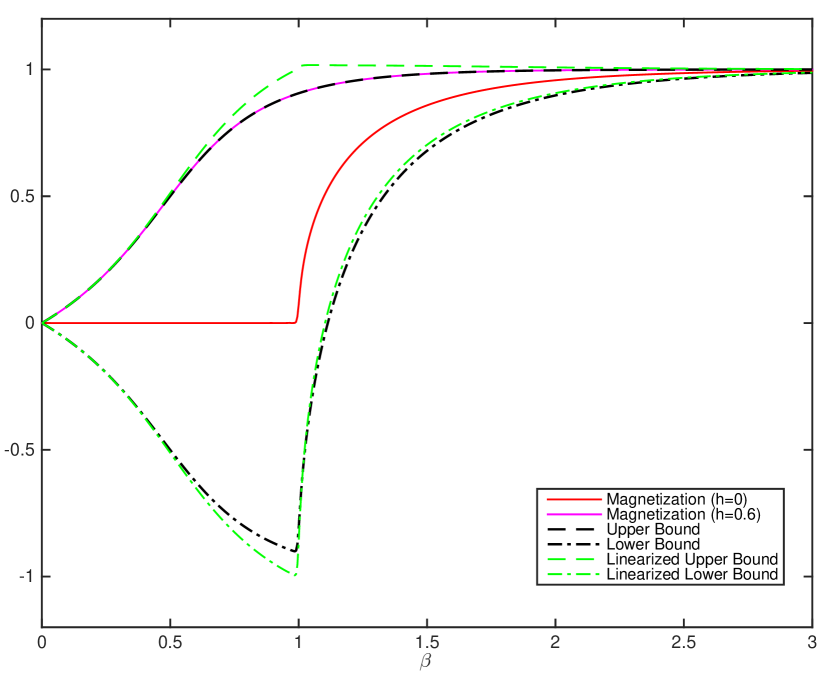
(a)

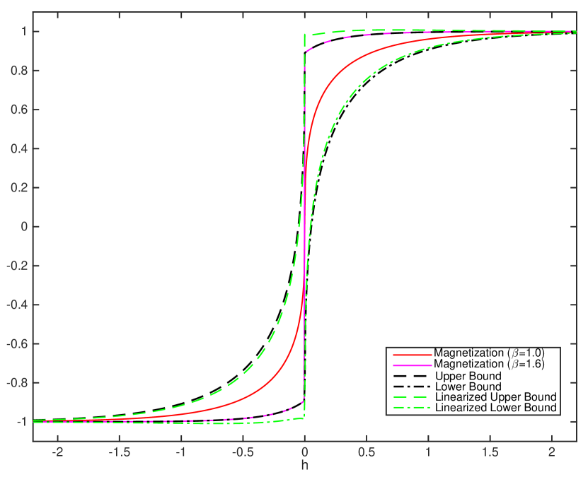
(b)

Figure 2: 2(a): The red solid line is the magnetization for $h=0$; The magenta solid line is the magnetization for $h=0.6$. The black dashed/dash-dot lines is the upper/lower UQ bounds given by the goal-oriented divergences of the magnetization (70) for $h=0.6$ . The green dashed/dash-dot line is the linearized upper/lower bound. 2(b): The red solid line is the magnetization for $\beta=1$; The magenta solid line is the magnetization for $\beta=1.6$. The black dashed/dash-dot lines is the upper/lower goal-oriented divergence bound of the magnetization for $\beta=1.6$ . The green dashed/dash-dot line is the linearized upper/lower bound.

(2a) One-dimensional Ising model versus mean field.  Consider the $1$-d Ising model and mean field model and assume $\mu_{N}$ and $\mu_{N;mf}$ are respectively their Gibbs distributions, which are defined in C.1 . Then, by straightforward calculations, we obtain

$$\lim\limits_{N}\frac{1}{N}R(\mu_{N}\|\mu_{N;mf}) =\log\frac{e^{\beta[h+Jm]}+e^{-\beta[h+Jm]}}{e^{\beta J}\cosh(\beta h)+k_{1}}+\frac{\beta J}{k_{1}}(k_{1}-\frac{2e^{-2\beta J}}{e^{\beta J}\cosh(\beta h)+k_{1}}-me^{J\beta}\sinh(h\beta))$$ (74)

where $k_{1}=\sqrt{e^{2J\beta}\sinh^{2}(h\beta)+e^{-2J\beta}}$; detailed calculations can be found in C.2 . By (72) and (73), we have

$$\frac{1}{N}\Lambda_{{N;mf},Nf_{N}}(c)=\log\frac{e^{[c+\beta(h+Jm)]}+e^{-[c+\beta(h+Jm)]}}{e^{-\beta[h+Jm]}+e^{\beta[h+Jm]}}.$$ (75)

and

$$\frac{1}{N}Var_{\mu_{N;mf}}(\sum_{x\in\Lambda_{N}}\sigma(x)) = 1-m^{2}.$$ (76)

Combining with C.1, for given parameters, we can calculate the magnetizations, the goal-oriented divergence bounds and their corresponding linearized approximation.

In Figure 3(a), we set $h=0$ and $J=1$ and consider the Gibbs measure of the mean field model as the benchmark, that is we use it as a surrogate model for the Ising model. In the figure, we see that its magnetization vanishes at high temperatures. At low temperatures it goes to its maximum value $m=1$, exhibiting spontaneous magnetization and a phase transition at the inverse temperature $\beta=1$. We plot the upper/lower goal-oriented divergence bound as well as their corresponding linearized bounds of the magnetization as a function of $\beta$. To test the sharpness of these bounds, we also plot the magnetization of the Ising model in the figure. The magnetization of the Ising model vanishes for all temperatures, exhibiting no phase transitions. In this sense the mean field approximation of the Ising model is a very poor one and the UQ bounds depicted in Figure 3(a) capture and quantify the nature of this approximation. Indeed, we can see that the bounds work well here, but the linearized lower bound fails for low temperatures because of the considerable difference between $\mu_{N}$ and $\mu_{N;mf}$. In Figure 3(b), we set $\beta=1$ and $J=1$ and consider the bounds and the magnetizations as a function of the external field $h$. Similarly with Figure 3(a), we take the Gibbs measure of the mean field model as the benchmark. To test the sharpness of the bounds, we also plot the magnetization of the Ising model in the figure. We can see the goal-oriented divergence bounds of the magnetization of the Ising model works well here. The upper bound almost coincides with it for positive $h$ and the lower bound almost coincide with it for negative $h$. However, the linearized ones do not give a good approximation around the point $h=0$.

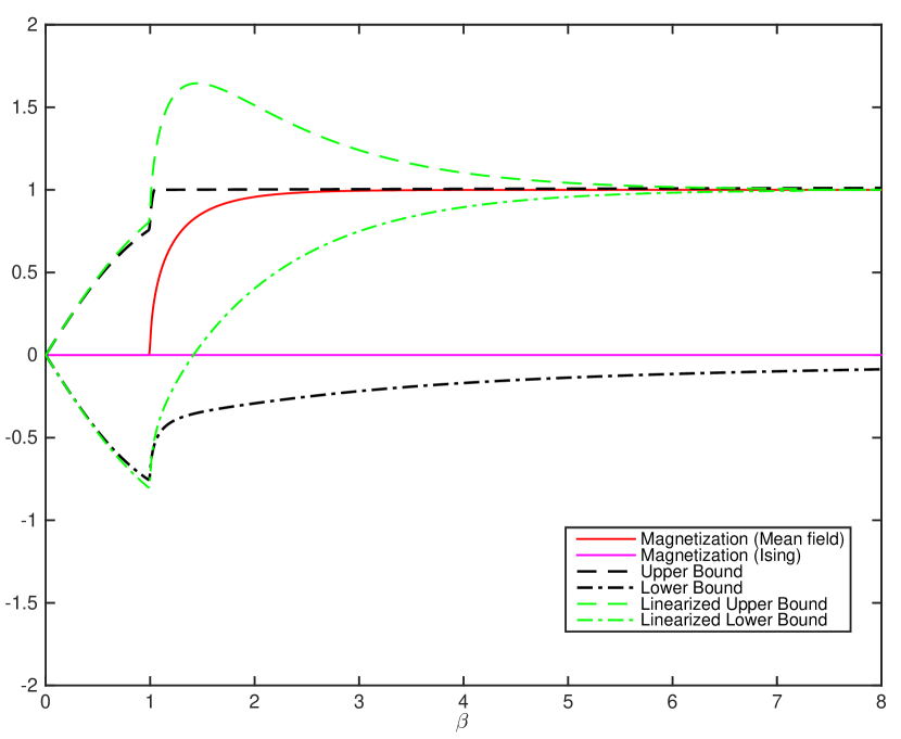
(a)

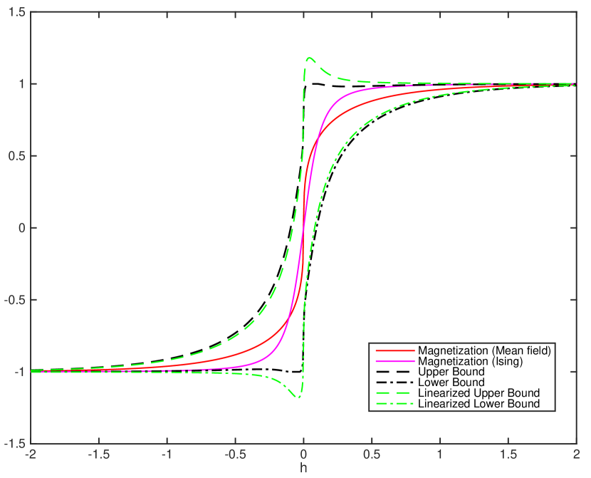
(b)

Figure 3: 3(a):The red solid line is the magnetization of 1-d mean field model for $h=0$; The magenta solid line is the magnetization of 1-d Ising model for $h=0$. The black dashed/dash-dot lines is the upper/lower goal-oriented divergence bound of the magnetization of the Ising model. The green dashed/dash-dot line is the linearized upper/lower bound. 3(b):The red solid line is the magnetization of 1-d mean field model for $\beta=1.0$; The magenta solid line is the magnetization of 1-d Ising model $\beta=1.0$. The black dashed/dash-dot lines is the upper/lower goal-oriented divergence bound of the magnetization of the Ising model. The green dashed/dash-dot line is the linearized upper/lower bound.

(2b) Two-dimensional Ising model versus mean field.  We revisit the example in (2a) above but this time in two dimensions where the Ising model exhibits phase transitions at a finite temperature. WE denote by $\mu_{N}$ and $\mu_{N;mf}$ the Gibbs distributions for the two-dimensional zero-field Ising model and two-dimensional mean field model with $h_{mf}=2Jm$, respectively. Then, by straightforward calculations, we obtain

$$\lim\limits_{N}\frac{1}{N}R(\mu_{N}\|\mu_{N;mf}) = \log[e^{-2\beta Jm}+e^{2\beta Jm}]-\frac{\log 2}{2}-\frac{1}{2\pi}\int_{0}^{\pi}\log[\cosh^{2}(2\beta J)+k(\theta)]d\theta$$ (77)

$$+ \beta J\frac{\sinh(4\beta J)}{\pi}\int_{0}^{\pi}\frac{1}{k(\theta)}[1-\frac{1+\cos(2\theta)}{\cosh^{2}(2\beta J)+k(\theta)}]d\theta-2\beta JmM_{0},$$

$$\frac{1}{N}\Lambda_{\mu_{N;mf},Nf_{N}}(c)=\log\frac{e^{(c+2\beta Jm)}+e^{-(c+2\beta Jm)}}{e^{-2\beta Jm}+e^{2\beta Jm}}$$ (78)

and

$$\frac{1}{N}Var_{\mu_{N;mf}}(\sum_{x\in\Lambda_{N}}\sigma(x)) = 1-m^{2},$$ (79)

where $m$ and $M_{0}$ are the spontaneous magnetizations of the two-dimensional mean field model and Ising models, respectively and can be obtain by solving (110) and (C.1). Detailed calculations can be found in C.2. Combining with C.1, for given parameters, we can calculate the magnetizations, the goal-oriented divergence bounds and their corresponding linearized approximation.

In Figure 4(a), we set $h=0$ and $J=1$ and plot the bounds and the magnetizations as a function of inverse temperature $\beta$. Similarly with Figure 3, we take the Gibbs measure of the mean field as the benchmark and consider the bounds for the magnetization of the Ising model. We can see that the goal-oriented bounds work well here, especially in low temperatures. Notice the large uncertainty prior to the onset of the spontaneous magnetization (phase transition) which is due to a pitchfork bifurcation and the two branches (upper and lower) reported in Figure 1b, as well as in the panels in Figure 4. The linearized bounds also work well, but they are not as sharp as the goal-oriented divergence bounds around the critical points because of the larger value of the relative entropy $R(\mu_{N}\|\mu_{N;mf})$. There are phase transitions for both mean field model and Ising model. The critical points are $1/2$ and $\log(1+\sqrt{2})/2$ for mean field model and Ising model, respectively. Both their magnetizations vanish at high temperatures and go to their maximum values $1$ at low temperature.

Actually, the spontaneous magnetizations we consider in Figure 4(a) are both based on the definition $M=\lim\limits_{h\to 0^{+}}\langle\sigma(x)\rangle$. If we consider the definition $M=\lim\limits_{h\to 0^{-}}\langle\sigma(x)\rangle$, we can obtain another figure which is Figure 4(b). We can see the quantities in Figure 4(b) are just the opposite of the corresponding quantities in Figure 4(a). Combining both figures gives us the uncertainty region reported in the Introduction.

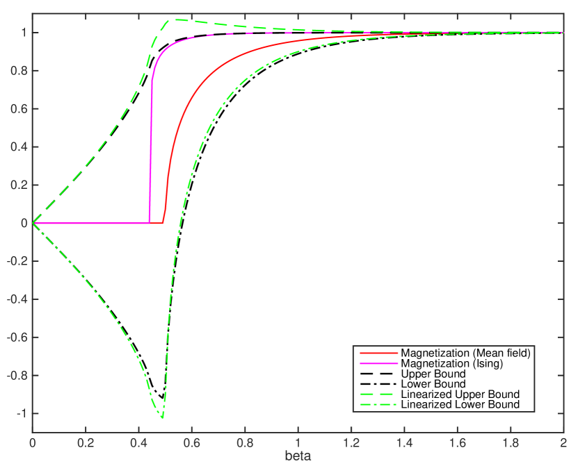
(a)

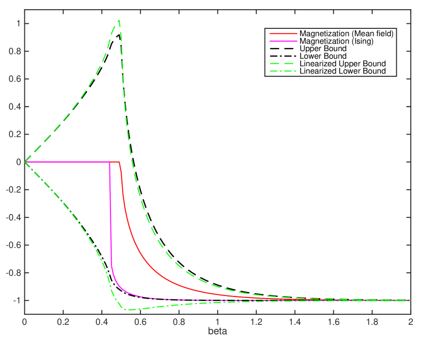
(b)

Figure 4: 4(a) The red solid line is the spontaneous magnetization of the 2-d mean field model with $h=0^{+}$; The magenta solid line is the spontaneous magnetization of 2-d Ising model with $h=0^{+}$; The black dashed/dash-dot lines is the upper/lower goal-oriented divergence bound of the magnetization for Ising model; The green dashed/dash-dot line is the linearized upper/lower bound. 4(b) The red solid line is the spontaneous magnetization of 2-d mean field model with $h=0^{-}$; The magenta solid line is the spontaneous magnetization of 2-d Ising model with $h=0^{-}$; The black dashed/dash-dot lines is the upper/lower goal-oriented divergence bound of the magnetization for Ising model; The green dashed/dash-dot line is the linearized upper/lower bound.

(3) One-dimensional Ising model versus Ising model.  Consider two one-dimensional Ising models and $\mu_{N}$ and $\mu_{N}^{\prime}$ are their Gibbs distributions defined in C.1. By straightforward calculation, we have

$$\lim\limits_{N}\frac{1}{N}R(\mu^{\prime}_{N}\|\mu_{N}) =\log\frac{e^{\beta J}\cosh(\beta h)+\sqrt{e^{2J\beta}\sinh^{2}(h\beta)+e^{-2J\beta}}}{e^{\beta^{\prime}J^{\prime}}\cosh(\beta^{\prime}h^{\prime})+\sqrt{e^{2J^{\prime}\beta^{\prime}}\sinh^{2}(h^{\prime}\beta^{\prime})+e^{-2J^{\prime}\beta^{\prime}}}}$$

$$+(\beta^{\prime}J^{\prime}-\beta J)(1-\frac{1}{k^{\prime}_{1}}\frac{2e^{-2\beta^{\prime}J^{\prime}}}{e^{\beta^{\prime}J^{\prime}}\cosh(\beta^{\prime}h^{\prime})+k^{\prime}_{1}})+(\beta^{\prime}h^{\prime}-\beta h)\frac{1}{k^{\prime}_{1}}e^{J^{\prime}\beta^{\prime}}\sinh(h^{\prime}\beta^{\prime})$$ (80)

and

$$\lim\limits_{N}\frac{1}{N}Var_{\mu_{N}}(\sum_{x\in\Lambda_{N}}\sigma(x))=\frac{1}{k_{1}^{3}}e^{-J\beta}\cosh(h\beta),$$ (81)

where $k^{\prime}_{1}=\sqrt{e^{2J^{\prime}\beta^{\prime}}\sinh^{2}(h^{\prime}\beta^{\prime})+e^{-2J^{\prime}\beta^{\prime}}}$. The cumulant generating function is

$$\lim\limits_{N}\frac{1}{N}\Lambda_{\mu_{N}}(c) = \log\frac{e^{\beta J}\cosh(\beta h+c)+\sqrt{e^{2J\beta}\sinh^{2}(h\beta+c)+e^{-2J\beta}}}{e^{\beta J}\cosh(\beta h)+\sqrt{e^{2J\beta}\sinh^{2}(h\beta)+e^{-2J\beta}}},$$ (82)

detailed calculations can be found in C.2. Combining with C.1, for given parameters, we can calculate the magnetizations, the bounds given by goal-oriented divergence and their corresponding linearized approximation.

In Figure 5(a), we set $J=1$ and plot the magnetizations of 1-d Ising model as a function of inverse temperature $\beta$ for $h=0$ and $h=0.6$, respectively. For the zero-field Ising model, used here as our benchmark, the magnetization vanishes for all temperatures. For $h=0.6$, the magnetization increases gradually to its maximum $1$. Clearly the models are far apart but the UQ bounds work remarkably well. Indeed, we plot the upper/lower goal-oriented divergence bound of the magnetization for the nonzero-field Ising model. The upper bound almost coincides with the magnetization itself. The lower bound is poor due to the symmetry of the bounds in $h$. If we break the symmetry by comparing models for different positive external fields both bounds become much sharper (not shown). The linearized bounds give a good approximation at high temperatures. However, at low temperatures, they are not as sharp as the goal-oriented divergence bounds. This is due to the larger relative entropy $R(\mu\|\mu^{\prime})$ between $\mu$ and $\mu^{\prime}$. In Figure 5(b), we plot the magnetization of the one-dimensional Ising model as a function of $h$ for two different inverse temperatures $\beta=1$ and $\beta=1.6$. The parameter $J$ was set to $1$. We also plot the upper/lower goal-oriented divergence bounds for $\beta=1.6$. Similarly with Figure 5(a), we also plot the linearized upper/lower bound in the figure. The goal-oriented divergence bounds work well here. We can see the upper bound almost coincides with the magnetization when $h$ is positive and the lower bound almost coincides with the magnetization when $h$ is negative. The linearized bounds make a relatively poor estimation around the since models are far apart due to the large perturbation in the parameter $\beta$ or $h$ in Figure 5.

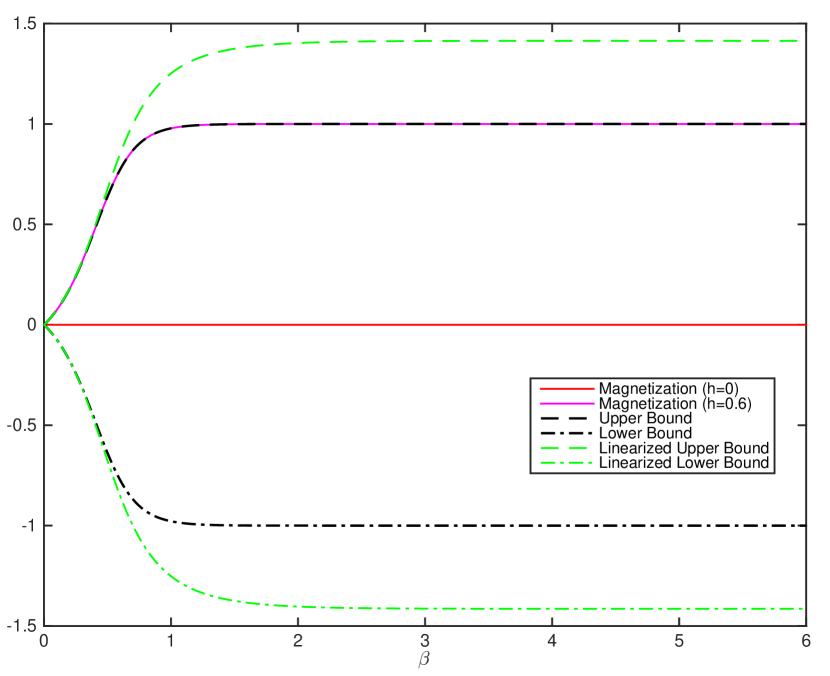
(a)

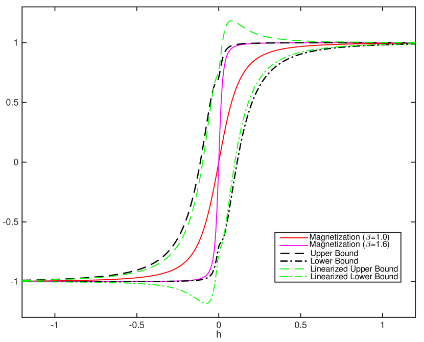
(b)

Figure 5: 5(a) The red solid line is the magnetization of 1-d Ising model for $h=0$; the magenta solid line is the magnetization of 1-d Ising model for $h=0.6$; the black dashed/dash-dot lines is the upper/lower bound by goal-oriented divergence; the green dashed/dash-dot line is the linearized upper/lower bound. 5(b) The red solid line is the magnetization of 1-d Ising model for $\beta=1$; the magenta solid line is the magnetization of 1-d Ising model for $\beta=1.6$; the black dashed/dash-dot lines is the upper/lower bound by goal-oriented divergence; the green dashed/dash-dot line is the linearized upper/lower bound.

7 Conclusions

In this paper we first showed that the classical information inequalities such as Pinsker-typer inequalities and other inequalities based on the Hellinger distance, the $\chi^{2}$-divergence, or the R$\acute{e}$nyi divergence perform poorly for the purpose of controlling QoIs of systems with many degrees of freedom, and/or in long time regimes. On the other hand we demonstrated that the goal oriented divergence introduced in [33] scales properly and allows to control QoIs provided they can be written as ergodic averages or spatial averages, e.g. quantities like autocorrelation, mean magnetization, specific energy, and so on. We illustrated the potential of our approach by computing uncertainty quantification bounds for phase diagrams for Gibbs measures, that is for systems in the thermodynamic limit. We showed that the bounds perform remarkably well even in the presence of phase transitions.

Although we provided computable bounds and exact calculations, there is still a lot to be done towards developing efficient Monte Carlo samplers for the goal oriented divergences $\Xi_{\pm}$, which is a central mathematical object in our approach. An additional strength of our approach is that it also applies to non-equilibrium systems which do not necessarily satisfy detailed balance, providing robust nonlinear response bounds. The key insight here is to study the statistical properties of the paths of the systems and to use the thermodynamic formalism for space-time Gibbs measures. Our results can be applied to a wide range of problems in statistical inference, coarse graining of complex systems, steady states sensitivity analysis for non-equilibrium systems, and Markov random fields.

Reference

Appendix A Hellinger-based Inequalities

Lemma A.1.

Suppose $P$ and $Q$ be two probability measures on some measure space $(\mathcal{X},\mathcal{A})$ and let $f:\mathcal{X}\to\mathbb{R}$ be some quantity of interest (QoI), which is measurable and has second moments with respect to both $P$ and $Q$. Then

$$\left|E_{Q}(f)-E_{P}(f)\right| \leq \sqrt{2}H(Q,P)\sqrt{Var_{P}(f)+Var_{Q}(g)+\frac{1}{2}(E_{Q}(f)-E_{P}(f))^{2}}.$$ (83)

Proof.

By Lemma $7.14$ in [41],we have

$$\left|E_{Q}(f)-E_{P}(f)\right| \leq \sqrt{2}H(Q,P)\sqrt{E_{P}(f^{2})+E_{Q}(f^{2})}.$$

For any $c\in\mathbb{R}$, replace $f$ by $f-c$, we have

$$\mid E_{Q}(f)-E_{P}(f)\mid =\mid E_{P}(f-c)-E_{Q}(f-c)\mid$$

$$\leq\sqrt{2}H(Q,P)\sqrt{E_{P}((f-c)^{2})+E_{Q}((f-c)^{2})}.$$

Thereby,

$$\mid E_{Q}(f)-E_{P}(f)\mid\leq\inf\limits_{c}\sqrt{2}H(Q,P)\sqrt{E_{P}((f-c)^{2})+E_{Q}((f-c)^{2})}$$

By some straight calculations, we can find the optimal c is :

$$c^{\star}=\frac{E_{P}(f)+E_{Q}(f)}{2}.$$

Thus, we have

$$\mid E_{Q}(f)-E_{P}(f)\mid \leq \sqrt{2}H(Q,P)\sqrt{E_{Q}[(f-c^{\star})^{2}]+E_{P}[(f-c^{\star})^{2}]}$$

$$= \sqrt{2}H(Q,P)\sqrt{Var_{P}(f)+Var_{Q}(g)+\frac{1}{2}(E_{Q}(f)-E_{P}(f))^{2}}.$$

Appendix B Proof of Lemmas 2.1 and 2.2

B.1 I.I.D. sequences

Proof of Lemma 2.1. since $P_{N}$ and $Q_{N}$ are product measures we have $\frac{dP_{N}}{dQ_{N}}(\sigma_{\Lambda_{N}})=\prod_{j=1}^{N}\frac{dP}{dQ}(\sigma_{j})$.

For the relative entropy we have

$$R(P_{N}\mid\mid Q_{N}) = \int_{\mathcal{X}_{n}}\log\frac{dP_{N}}{dQ_{N}}(\sigma_{\Lambda_{N}})dP_{N}(\sigma_{\Lambda_{N}})=\int_{\mathcal{X}_{n}}\sum_{j=1}^{N}\log\frac{dP}{dQ}(\sigma_{j})dP_{N}(\sigma_{\Lambda_{N}})$$ (84)

$$= \sum_{j=1}^{N}\int_{\mathcal{X}}\log\frac{dP}{dQ}(\sigma_{j})dP(\sigma_{j})=NR(P\mid\mid Q)\,.$$

For the Reny relative entropy we have

$$D_{\alpha}(P_{N}\mid\mid Q_{N}) = \log\int_{\mathcal{X}_{n}}\left(\frac{dP_{N}}{dQ_{N}}(\sigma_{\Lambda_{N}})\right)^{\alpha}dQ_{N}(\sigma_{\Lambda_{N}})=\log\int_{\mathcal{X}_{n}}\prod_{j=1}^{N}\left(\frac{dP}{dQ}(\sigma_{j})\right)^{\alpha}dQ_{N}(\sigma_{\Lambda_{N}})$$ (85)

$$= \sum_{j=1}^{N}\log\int_{\mathcal{X}}\left(\frac{dP}{dQ}(\sigma_{j})\right)^{\alpha}dQ(\sigma_{j})=ND_{\alpha}(P\mid\mid Q)\,.$$

For the $\chi^{2}$ distance we note first that

$$\chi^{2}(P\mid\mid Q)=\int\left(\frac{dP}{dQ}-1\right)^{2}dQ=\int\left(\left(\frac{dP}{dQ}\right)^{2}-2\frac{dP}{dQ}+1\right)dQ=\int\left(\frac{dP}{dQ}\right)^{2}dQ-1\,,$$

and therefore we have

$$\chi^{2}(P_{N}\mid\mid Q_{N}) = \int_{\mathcal{X}_{n}}\left(\prod_{j=1}^{N}\frac{dP}{dQ}(\sigma_{j})\right)^{2}dQ_{N}(\sigma_{\Lambda_{N}})-1=\prod_{j=1}^{N}\int_{\mathcal{X}}\left(\frac{dP}{dQ}(\sigma_{j})\right)^{2}dQ(\sigma_{j})-1$$ (86)

$$= \left(1+\chi^{2}(P\mid\mid Q)\right)^{N}-1\,.$$

For the Hellinger distance we note first that

$$H^{2}(P,Q)=\int\left(\sqrt{\frac{dP}{dQ}}-1\right)^{2}dQ=\int\left(\frac{dP}{dQ}-2\sqrt{\frac{dP}{dQ}}+1\right)dQ=2-2\int\sqrt{\frac{dP}{dQ}}dQ\,,$$

and thus $\int\sqrt{\frac{dP}{dQ}}dQ=1-\frac{1}{2}H^{2}(P,Q)$. Therefore we have

$$H^{2}(P_{N},Q_{N}) = 2-2\int_{\mathcal{X}_{n}}\sqrt{\prod_{j=1}^{N}\frac{dP}{dQ}(\sigma_{j})}dQ(\sigma_{\Lambda_{N}})=2-2\prod_{j=1}^{N}\int_{\mathcal{X}}\sqrt{\frac{dP}{dQ}(\sigma_{j})}dQ(\sigma_{j})$$ (87)

$$= 2-2\left(1-\frac{H^{2}(P,Q)}{2}\right)^{N}\,.$$

This concludes the proof of Lemma 2.1.

B.2 Markov sequences

Proof of Lemma 2.2: The convergence of the relative entropy rate is well known and we give here a short proof for the convenience of the reader.

Recall that $\nu_{p}$ and $\nu_{q}$ are the initial distributions of the Markov chain at time $0$ with transition matrices $p$ and $q$ respectively. We write $\nu_{p}^{k}$ the distribution at time $k$ as a row vector and we have then $\nu_{p}^{k}(x)\equiv\nu_{p}p^{k}(x)$ where $p^{k}$ is the matrix product.

By expanding the logarithm and integrating we find

$$\frac{1}{N}\int\log\frac{dP_{N}}{dQ_{N}}dP_{N}$$

$$=\frac{1}{N}\sum_{x_{0},\cdots x_{N}}\log\left(\frac{\nu_{p}(x_{0})p(x_{0},x_{1})\cdots p(x_{n-1},x_{n})}{\nu_{q}(x_{0})q(x_{0},x_{1})\cdots q(x_{n-1},x_{n})}\right)\nu_{p}(x_{0})p(x_{0},x_{1})\cdots p(x_{n-1},x_{n})$$

$$=\frac{1}{N}\sum_{x_{0}}\log\frac{\nu_{p}(x_{0})}{\nu_{q}(x_{0})}\nu_{p}(x_{0})+\frac{1}{N}\sum_{k=1}^{N}\sum_{x_{0},\cdots,x_{k}}\nu_{p}(x_{0})p(x_{0},x_{1})\cdots p(x_{k-1},x_{k})\log\frac{p(x_{k-1},x_{k})}{q(x_{k-1},x_{k})}$$

$$=\frac{1}{N}\sum_{x_{0}}\log\frac{\nu_{p}(x_{0})}{\nu_{q}(x_{0})}\nu_{p}(x_{0})+\frac{1}{N}\sum_{k=1}^{N}\sum_{x,y}\nu_{p}^{k}(x)p(x,y)\log\frac{p(x,y)}{q(x,y)}.$$ (88)

The first term goes to $0$ as $N\to\infty$ while for the second term, by the ergodic theorem we have that for any initial condition $\nu_{p}$, $\lim_{N\to\infty}\frac{1}{N}\sum_{k=1}^{N}\nu_{p}^{k}=\mu_{p}$ where $\mu_{p}$ is stationary distribution. Therefore we obtain that

$$\lim_{N\to\infty}\frac{1}{N}\int\log\frac{dP_{N}}{dQ_{N}}dP_{N}=\sum_{x,y}\mu_{p}(x)p(x,y)\log\frac{p(x,y)}{q(x,y)}.$$

Finally we note that the limit can be written as a relative entropy itself, since

$$\sum_{x,y}\mu_{p}(x)p(x,y)\log\frac{p(x,y)}{q(x,y)}=\sum_{x}\mu_{p}(x)R\left(p(x,\cdot)\mid\mid q(x,\cdot)\right).$$

As a consequence the relative entropy rate vanishes if and only if $R\left(p(x,\cdot)\mid\mid q(x,\cdot)\right)=0$ for every $x$ that is if and only if $p(x,y)=q(x,y)$ for every $x$ and $y$.

We turn next to R$\acute{e}$nyi entropy. As it will turn out understanding the scaling properties of the R$\acute{e}$nyi entropy will allow us immediately to understand the scaling properties of the chi-squared and Hellinger divergences as well. We have

$$\frac{1}{N}D_{\alpha}(P_{N}\mid\mid Q_{N})=\frac{1}{N}\frac{1}{\alpha-1}\log\sum_{x_{0},\cdots x_{N}}\nu_{q}(x_{0})^{1-\alpha}\nu_{p}(x_{0})^{\alpha}\prod_{j=1}^{N}p(x_{j-1},x_{j})^{\alpha}q(x_{j-1},x_{j})^{1-\alpha}.$$

Let $F_{\alpha}$ be the non-negative matrix with entries

$$F_{\alpha}(x,y)=p(x,y)^{\alpha}q(x,y)^{1-\alpha}.$$

since $p$ and $q$ are irreducible and mutually absolutely continuous the matrix $F_{\alpha}$ is irreducible as well. Let $v$ be the row vector with entries $v(x)=\nu_{q}(x)^{1-\alpha}\nu_{p}(x)$ and $1$ the column vector with all entries equal to $1$. Then we have

$$\frac{1}{N}D_{\alpha}(P_{N}\mid\mid Q_{N})=\frac{1}{\alpha-1}vF_{\alpha}^{N}1,$$

and thus by the Perron-Frobenius Theorem [50], we have

$$\lim_{N\to\infty}\frac{1}{N}D_{\alpha}(P_{N},Q_{N})=\frac{1}{\alpha-1}\log\rho(\alpha).$$

where $\rho(\alpha)$ is the maximal eigenvalue of the non-negative matrix $F_{\alpha}$.

It remains to show that the limit is $0$ only if $p=q$. In order to do this we will use some convexity properties of the R$\acute{e}$nyi entropy [38]. For $0<\alpha\leq 1$ the R$\acute{e}$nyi entropy $D_{\alpha}(P\mid\mid Q)$ is jointly convex in $P$ and $Q$, i.e. for any $\epsilon\in[0,1]$ we have

$$D_{\alpha}(\epsilon P_{0}+(1-\epsilon)P_{1}\mid\mid\epsilon Q_{0}+(1-\epsilon)Q_{1})\leq\epsilon D(P_{0}\mid\mid Q_{0})+(1-\epsilon)D(P_{1}\mid\mid Q_{1}).$$

For $\alpha>1$ the R$\acute{e}$nyi entropy is merely jointly quasi-convex, that is

$$D_{\alpha}(\epsilon P_{0}+(1-\epsilon)P_{1}\mid\mid\epsilon Q_{0}+(1-\epsilon)Q_{1})\leq\max\left\{D(P_{0}\mid\mid Q_{0}),D(P_{1}\mid\mid Q_{1})\right\}.$$

In any case let us assume that $p\not=q$ is such that

$$\lim_{N\to\infty}\frac{1}{N}D_{\alpha}(P_{N}\mid\mid Q_{N})=0\,.$$

Then by convexity, or quasi-convexity we have for any $\epsilon\in[0,1]$

$$\lim_{N\to\infty}\frac{1}{N}D_{\alpha}(\epsilon P_{N}+(1-\epsilon)Q_{N}\mid\mid Q_{N})=0\,.$$

On the other hand, for any smooth parametric family $Q_{\theta}$ we have that, [38],

$$D_{\alpha}(Q^{\theta^{\prime}}\mid\mid Q^{\theta})=\frac{\alpha}{2}(\theta-\theta^{\prime})^{2}J(Q^{\theta})+O((\theta^{\prime}-\theta)^{3})$$

where $J(Q^{\theta})$ is the Fisher information. If $Q^{\theta}$ is a discrete probability distribution then the Fisher information is $J(Q^{\theta})=\sum_{x}Q^{\theta}(x)(\frac{d}{d\theta}\log Q^{\theta}(x))^{2}$.

To compute $J(Q_{N}^{\theta})$ we can use the relative entropy $R(Q_{N}^{\theta^{\prime}}\mid\mid Q_{N}^{\theta})=D_{1}(Q_{N}^{\theta^{\prime}}\mid\mid Q_{N}^{\theta})$ and from (88) with $q=q^{\theta}$ and $p=q^{\theta^{\prime}}$ we obtain

$$R(Q^{\theta^{\prime}}_{N}\mid\mid Q^{\theta}_{N}) = (\theta^{\prime}-\theta)^{2}\sum_{x}\nu_{q^{\theta}}(x)\left(\frac{d}{d\theta}\log\nu_{q^{\theta}}(x)\right)^{2}$$

$$+\frac{1}{2}(\theta-\theta^{\prime})^{2}\sum_{k=1}^{N}\sum_{x,y}(\nu_{q^{\theta}})^{k}(x)q^{\theta}(x,y)\left(\frac{d}{d\theta}\log q^{\theta}(x,y)\right)^{2}+O((\theta-\theta^{\prime})^{3}).$$

So as $N\to\infty$ we obtain

$$\lim_{N\to\infty}\frac{1}{N}R(Q_{N}^{\theta^{\prime}}\mid\mid Q_{N}^{\theta})=\frac{1}{2}(\theta-\theta^{\prime})^{2}\sum_{x,y}\mu_{q^{\theta}}(x)q^{\theta}(x,y)\left(\frac{d}{d\theta}\log q^{\theta}(x,y)\right)^{2}+O((\theta-\theta^{\prime})^{3})$$ (89)

If we now apply this to the family $Q^{\epsilon}=Q_{N}+\epsilon(P_{N}-Q_{N})$ we have that

$$\lim_{N\to\infty}\frac{1}{N}R(Q_{N}+\epsilon(P_{N}-Q_{N})\mid\mid Q_{N})=\frac{1}{2}\epsilon^{2}\sum_{x,y}\mu_{q}(x)\frac{(p(x,y)-q(x,y))^{2}}{q(x,y)}+O(\epsilon^{3})$$

since the term of order $\epsilon^{2}$ is strictly positive unless $p=q$ this contradicts our assumption that $\lim_{N\to\infty}\frac{1}{N}D_{\alpha}(\epsilon P_{N}+(1-\epsilon)Q_{N}\mid\mid Q_{N})=0$.

We can now easily deduce the scaling of the $\chi^{2}$ divergence from the R$\acute{e}$nyi relative entropy because of the relation $\chi^{2}(Q_{N}\mid\mid P_{N})=e^{D_{2}(Q_{N}\mid\mid P_{N})}-1$. This implies that $\chi^{2}(Q_{N}\mid\mid P_{N})$ grows exponentially in $N$ unless $\lim_{N\to\infty}\frac{1}{N}D_{2}(Q_{N}\mid\mid P_{N})=0$ which is possible if and only if $p=q$.

Similarly for the Hellinger distance we use the relation $H^{2}(P_{N},Q_{N})=2-2e^{-\frac{1}{2}D_{\frac{1}{2}}(Q_{N}\mid\mid P_{N})}$ and the scaling of the R$\acute{e}$nyi entropy to see $H(Q_{N},P_{N})$ converges to $\sqrt{2}$ unless $p=q$. This concludes the proof of Lemma 2.2.

Appendix C Background for Section 5

C.1 Ising models and mean field models

One-dimensional Ising model Consider an Ising model on the lattice $\Lambda_{N}$ which a line of N sites, labelled successively $x=1,2,...,N$. At each site there is a spin $\sigma(x)$, with two possible values: $+1$ or $-1$. The the Hamiltonian is given by

$$H_{N}(\sigma_{\Lambda_{N}})=-\beta J\sum_{x=1}^{N-1}\sigma(x)\sigma(x+1)-\beta h\sum_{x\in\Lambda_{N}}\sigma(x).$$ (90)

The configuration probability is given by the Boltzmann distribution with inverse temperature $\beta\geq 0$:

$$d\mu_{N}(\sigma_{\Lambda_{N}})=\frac{1}{Z_{N}}e^{-H_{N}(\sigma_{\Lambda_{N}})}dP_{N}(\sigma_{\Lambda_{N}}),$$ (91)

where

$$Z_{N}=\sum_{\sigma_{\Lambda_{N}}}e^{-H_{N}(\sigma_{\Lambda_{N}})}$$ (92)

is the partition function and $P_{N}(\sigma_{\Lambda_{N}})$ is the counting measure on $\Lambda_{N}$.

By [49], the magnetization is

$$M=\frac{e^{J\beta}\sinh(h\beta)}{\sqrt{e^{2J\beta}\sinh^{2}(h\beta)+e^{-2J\beta}}},$$ (93)

and the pressure is

$$P=\lim\limits_{N}\frac{1}{N}\log Z_{N}=\log[e^{\beta J}\cosh(\beta h)+\sqrt{e^{2J\beta}\sinh^{2}(h\beta)+e^{-2J\beta}}].$$ (94)

Differentiating (92) with respect to $J$ and using (94), one obtain

$$\lim\limits_{N}\frac{1}{N}E_{\mu_{N}}[\sum_{x\in\Lambda_{N}}\sigma(x)\sigma(x+1)]=\lim\limits_{N}\frac{1}{\beta}\frac{\partial}{\partial J}(\frac{1}{N}\log Z_{N})=1-\frac{1}{k_{1}}\frac{2e^{-2\beta J}}{e^{\beta J}\cosh(\beta h)+k_{1}},$$ (95)

where

$$k_{1}=\sqrt{e^{2J\beta}\sinh^{2}(h\beta)+e^{-2J\beta}}.$$ (96)

Consider the susceptibility $\mathcal{X}$, by Section 1.7 in [49], we have

$$\mathcal{X}=\frac{\partial M}{\partial h}=\beta\lim\limits_{N}\frac{1}{N}Var_{\mu_{N}}(\sum_{x\in\Lambda_{N}}\sigma(x)).$$ (97)

Thus, by differentiating (93) with respect to h, we obtain

$$\lim\limits_{N}\frac{1}{N}Var_{\mu_{N}}(\sum_{x\in\Lambda_{N}}\sigma(x))=\frac{e^{-J\beta}\cosh(h\beta)}{k_{1}^{3}}.$$ (98)

Square lattice zero-field Ising model Consider an Ising model on the square lattice $\Lambda_{N}$ with $|\Lambda|=N$. Similarly with the 1-d Ising model, the spins $\{\sigma(x)\}_{x=1}^{N}\in\{-1,1\}^{N}$. Assume there is no external magnetic field, then Hamiltonian for the 2-d zero-field Ising model is given by

$$H_{N}(\sigma_{\Lambda_{N}})=-\beta J\sum_{\langle x,y\rangle\subset\Lambda_{N}}\sigma(x)\sigma(y).$$ (99)

where the first sum is over pairs of adjacent spins (every pair is counted once). The notation $\langle x,y\rangle$ indicates that sites $x$ and $y$ are nearest neighbors. Then the configuration probability is given by:

$$d\mu_{N}(\sigma_{\Lambda_{N}})=\frac{1}{Z_{N}}e^{\beta J\sum_{\langle x,y\rangle\subset\Lambda_{N}}\sigma(x)\sigma(y)}dP_{N}(\sigma_{\Lambda_{N}}),$$ (100)

where

$$Z_{N}=\sum_{\sigma_{\Lambda_{N}}}e^{\beta J\sum_{\langle x,y\rangle\subset\Lambda_{N}}\sigma(x)\sigma(y)}$$ (101)

is the partition function and $P_{N}(\sigma_{\Lambda_{N}})=\prod_{x=1}^{N}P(\sigma_{\Lambda_{N}})$ is the prior distribution with $P(\sigma(x)=1)=P(\sigma(x)=-1)=0.5$. By Section 7.10 in [49], the spontaneous magnetization is

$$M_{0}=\begin{cases}[1-\sinh^{-4}(2\beta J)]^{1/8}&\text{ $\beta>\beta_{c}$ ,}\\ 0&\text{$\beta<\beta_{c}$,}\end{cases}$$

where $\beta_{c}=\frac{\log(1+\sqrt{2})}{2J}$. Actually, this formula for the spontaneous magnetization is given by the definition $M_{0}=\lim\limits_{h\to 0^{+}}\langle\sigma(x)\rangle$. Sometimes, we can also consider the spontaneous magnetization by using the other definition $M=\lim\limits_{h\to)^{-}}\langle\sigma(x)\rangle$, which actually is the opposite of (C.1).

And the pressure is also given by [49]

$$P=\lim\limits_{N\to\infty}\frac{1}{N}\log Z_{N}=\frac{\log 2}{2}+\frac{1}{2\pi}\int_{0}^{\pi}\log[\cosh^{2}(2\beta J)+k(\theta)]d\theta,$$ (102)

where

$$k(\theta)=\sqrt{\sinh^{4}(2\beta J)+1-2\sinh^{2}(2\beta J)\cos(2\theta)}.$$ (103)

And, by (101) and (102), we obtain

$$\lim\limits_{N\to\infty}\frac{1}{N}E_{\mu_{N}}(\sum_{\langle x,y\rangle\subset\Lambda_{N}}\sigma(x)\sigma(y))=\frac{1}{\beta}\frac{\partial}{\partial J}(\frac{1}{N}\log Z_{N})=\frac{\sinh(4\beta J)}{\pi}\int_{0}^{\pi}\frac{1}{k(\theta)}[1-\frac{1+\cos(2\theta)}{\cosh^{2}(2\beta J)+k(\theta)}]d\theta.$$ (104)

Mean field model Given the Lattice $\Lambda_{N}$ in d-dimension and set $|\Lambda|=N$, consider the Hamiltonian for d-dimensional Ising model

$$H_{N}(\sigma_{\Lambda_{N}})=-\beta J\sum_{\langle x,y\rangle\subset\Lambda_{N}}\sigma(x)\sigma(y)-\beta h\sum_{x\in\Lambda_{N}}^{N}\sigma(x)\\ =-\sum_{x\in\Lambda_{N}}\sigma(x)\{\frac{1}{2}\beta J\sum_{y}^{n.n}\sigma(y)+\beta h\},$$

where the first sum is over pairs of adjacent spins (every pair is counted once). The notation $\langle x,y\rangle$ indicates that sites $x$ and $y$ are nearest neighbors. And, $\{\sigma(x)\}_{x=1}^{N}\in\{-1,1\}^{N}$ are Ising spins. Replace $\sum_{y}^{n.n}\sigma(y)$ by $\sum_{y}^{n.n}\langle\sigma(y)\rangle$ in (C.1), we obtain the mean field Hamiltonian

$$H_{N;mf}(\sigma_{\Lambda_{N}}) = -\sum_{x\in\Lambda_{N}}\sigma(x)\{\frac{1}{2}\beta J\sum_{y}^{n.n}\langle\sigma(y)\rangle+\beta h\}$$

$$= -\sum_{x\in\Lambda_{N}}\sigma(x)\{\frac{1}{2}\beta J2dm+\beta h\}$$

$$= -\sum_{x\in\Lambda_{N}}\sigma(x)\{\beta Jdm+\beta h\}$$

$$= -\beta h_{mf}\sum_{x\in\Lambda_{N}}\sigma(x)$$

where $h_{mf}=h+Jdm$. Then, we have the probability

$$d\mu_{N;mf}(\sigma_{\Lambda_{N}})=\frac{1}{Z_{N;mf}}e^{-H_{N;mf}(\sigma_{\Lambda_{N}})}dP_{N}(\sigma_{\Lambda_{N}})=\frac{1}{Z_{N;mf}}e^{\beta\sum_{x\in\Lambda_{N}}h_{mf}\sigma(x)}dP_{N}(\sigma_{\Lambda_{N}}).$$ (106)

So the partition function is

$$Z_{N;mf} = \sum_{\sigma(x)}e^{\beta\sum_{x\in\Lambda_{N}}h_{mf}\sigma(x)}$$ (107)

$$= \sum_{\sigma(x)}\prod_{x\in\Lambda_{N}}e^{\beta h_{mf}\sigma(x)}$$

$$= \prod_{x\in\Lambda_{N}}\sum_{\sigma(x)}e^{\beta h_{mf}\sigma(x)}$$

$$= \prod_{x\in\Lambda_{N}}(e^{\beta h_{mf}}+e^{-\beta h_{mf}})$$

$$= (e^{\beta h_{mf}}+e^{-\beta h_{mf}})^{N}$$

$$= {Z_{1;mf}}^{N},$$

where $Z_{1;mf}=e^{\beta h_{mf}}+e^{-\beta h_{mf}}$. So the pressure is

$$P_{mf}=\lim\limits_{N}\frac{1}{N}\log Z_{N;mf}=\log(e^{\beta h_{mf}}+e^{-\beta h_{mf}})$$ (108)

And, we can also consider the $\mu_{N;mf}$ as a product measure

$$d\mu_{N;mf}(\sigma_{\Lambda_{N}})=\frac{1}{Z_{N;mf}}e^{\beta\sum_{x\in\Lambda_{N}}h_{mf}\sigma(x)}dP_{N}(\sigma_{\Lambda_{N}})=\prod_{x\in\Lambda_{N}}\frac{1}{Z_{1;mf}}e^{\beta h_{mf}\sigma(x)}dP(\sigma(x)).$$ (109)

It is easy to find the magnetization

$$m = \frac{1}{N}E_{\mu_{N;mf}}[\sum_{x\in\Lambda_{N}}\sigma(x)]$$ (110)

$$= \frac{1}{N}\sum_{x\in\Lambda_{N}}E_{\mu_{N;mf}}[\sigma(x)]$$

$$= \frac{1}{N}\sum_{x\in\Lambda_{N}}\sum_{\sigma(x)}\sigma(x)\frac{1}{Z_{1;mf}}e^{\beta h_{mf}\sigma(x)}$$

$$= \frac{1}{N}\sum_{x\in\Lambda_{N}}\sum_{\sigma(x)}\sigma(x)\frac{1}{Z_{1;mf}}e^{\beta h_{mf}\sigma(x)}$$

$$= \frac{1}{N}\sum_{x\in\Lambda_{N}}\frac{1}{Z_{1;mf}}(e^{\beta h_{mf}}-e^{-\beta h_{mf}})$$

$$= \frac{1}{e^{\beta h_{mf}}+e^{-\beta h_{mf}}}(e^{\beta h_{mf}}-e^{-\beta h_{mf}})$$

$$= \tanh(\beta h_{mf})$$

$$= \tanh(\beta h+\beta Jdm)$$

and

$$\frac{1}{N}Var_{\mu_{N;mf}}(\sum_{x\in\Lambda_{N}}\sigma(x)) = \frac{1}{N}Var_{\mu_{N;mf}}(\sum_{x\in\Lambda_{N}}\sigma(x))$$ (111)

$$= \frac{1}{N}(E_{\mu_{N;mf}}[\sum_{x\in\Lambda_{N}}\sigma(x)]^{2}-N^{2}m^{2})$$

$$= \frac{1}{N}(E_{\mu_{N;mf}}[\sum_{x\in\Lambda_{N}}\sigma^{2}(x)+\sum_{x\neq y}\sigma(x)\sigma(y)]-Nm^{2})$$

$$= \{\sum_{\sigma(x)}\sigma^{2}(x)\frac{1}{Z_{1;mf}}e^{\beta h_{mf}\sigma(x)}+(N-1)E_{\mu_{N;mf}}[\sigma(x)\sigma(y)]\}-Nm^{2}$$

$$= \{1+(N-1)m^{2}\}-Nm^{2}$$

$$= 1-m^{2}.$$

So we can obtain the magnetization $m$ by solving the implicit equation (110).

C.2 Computation of goal-oriented divergences

Mean field versus mean field Given two mean field models, assume $\mu_{N;mf}$ and $\mu^{\prime}_{N;mf}$ are their two configuration probabilities with

$$d\mu_{N;mf}(\sigma)=\frac{1}{Z_{N;mf}}e^{-H_{N;mf}(\sigma_{\Lambda_{N}})}dP_{N}(\sigma_{\Lambda_{N}})=\frac{1}{Z_{N;mf}}e^{\beta\sum_{x\in\Lambda_{N}}h_{mf}\sigma(x)}dP_{N}(\sigma_{\Lambda_{N}})$$ (112)

and

$$d\mu^{\prime}_{N;mf}(\sigma)=\frac{1}{Z^{\prime}_{N;mf}}e^{-H^{\prime}_{N;mf}(\sigma_{\Lambda_{N}})}dP_{N}(\sigma_{\Lambda_{N}})=\frac{1}{Z^{\prime}_{N;mf}}e^{\beta^{\prime}\sum_{x\in\Lambda_{N}}h^{\prime}_{mf}\sigma(x)}dP_{N}(\sigma_{\Lambda_{N}}).$$ (113)

where $h_{mf}=h+dJm$ and $h^{\prime}_{mf}=h^{\prime}+dJ^{\prime}m^{\prime}$. Then, by (59), the relative entropy between $\mu^{\prime}_{N;mf}$ and $\mu_{N;mf}$ is given by

$$R(\mu^{\prime}_{N;mf}\|\mu_{N;mf}) = \log Z_{N;mf}-\log Z^{\prime}_{N;mf}+E_{\mu^{\prime}_{N;mf}}[H_{N;mf}(\sigma_{\Lambda_{N}})-H^{\prime}_{N;mf}(\sigma_{\Lambda_{N}})]$$ (114)

$$= \log\frac{Z_{N;mf}}{Z^{\prime}_{N;mf}}+(\beta^{\prime}h^{\prime}_{mf}-\beta h_{mf})E_{\mu^{\prime}_{N;mf}}(\sum_{x\in\Lambda_{N}}\sigma(x))$$

$$= N\log\frac{Z_{1;mf}}{Z^{\prime}_{1;mf}}+(\beta^{\prime}h^{\prime}_{mf}-\beta h_{mf})Nm^{\prime}$$

$$= N\log\frac{e^{\beta h_{mf}}+e^{-\beta h_{mf}}}{e^{-\beta^{\prime}h^{\prime}_{mf}}+e^{\beta^{\prime}h^{\prime}_{mf}}}+N(\beta^{\prime}h^{\prime}_{mf}-\beta h_{mf})m^{\prime}.$$

Therefore, we have

$$\frac{1}{N}R(\mu^{\prime}_{N;mf}\|\mu_{N;mf})=\log\frac{e^{\beta h_{mf}}+e^{-\beta h_{mf}}}{e^{-\beta^{\prime}h^{\prime}_{mf}}+e^{\beta^{\prime}h^{\prime}_{mf}}}+(\beta^{\prime}h^{\prime}_{mf}-\beta h_{mf})m^{\prime}.$$ (115)

And, the cumulant generating function of $Nf_{N}=N\frac{1}{N}\sum_{x\in\Lambda_{N}}\sigma(x)=\sum_{x\in\Lambda_{N}}\sigma(x)$ is

$$\Lambda_{\mu_{N;mf},Nf_{N}}(c) = \log E_{\mu_{N;mf}}(e^{cN\frac{1}{N}\sum_{x\in\Lambda_{N}}\sigma(x)})$$ (116)

$$= \log\sum_{\sigma(x)}e^{cN\frac{1}{N}\sum_{x\in\Lambda_{N}}\sigma(x)}\frac{1}{Z_{N;mf}}e^{\beta h_{mf}\sum_{x\in\Lambda_{N}}\sigma(x)}$$

$$= \log\sum_{\sigma(x)}\frac{1}{Z_{N;mf}}e^{(c+\beta h_{mf})\sum_{x\in\Lambda_{N}}\sigma(x)}$$

$$= \log\sum_{\sigma(x)}\prod_{x\in\Lambda_{N}}\frac{1}{Z_{1;mf}}e^{(c+\beta h_{mf})\sigma(x)}$$

$$= \log\prod_{x\in\Lambda_{N}}\sum_{\sigma(x)}\frac{1}{Z_{1;mf}}e^{(c+\beta h_{mf})\sigma(x)}$$

$$= \log\prod_{x\in\Lambda_{N}}\frac{1}{Z_{1;mf}}\{e^{(c+\beta h_{mf})}+e^{-(c+\beta h_{mf})}\}$$

$$= N\log\frac{e^{(c+\beta h_{mf})}+e^{-(c+\beta h_{mf})}}{e^{-\beta h_{mf}}+e^{\beta h_{mf}}}.$$

Thus,

$$\frac{1}{N}\Lambda_{\mu_{N;mf},Nf_{N}}(c)=\log\frac{e^{(c+\beta h_{mf})}+e^{-(c+\beta h_{mf})}}{e^{-\beta h_{mf}}+e^{\beta h_{mf}}}.$$ (117)

Also, by (111), we have

$$\frac{1}{N}Var_{\mu_{N;mf}}(Nf_{N}) = 1-m^{2}.$$ (118)

One-dimensional Ising model versus mean field Consider the Ising model and mean field model in 1-d and assume $\mu_{N}$ and $\mu_{N;mf}$ are the configuration probabilities for 1-d Ising model and mean field model respectively, which are defined in section C.1. Then, by (59), the relative entropy between $\mu_{N}$ and $\mu_{N;mf}$ is

$$R(\mu_{N}\|\mu_{N;mf}) =\log Z_{N;mf}-\log Z_{N}+E_{\mu_{N}}(H_{N;mf}(\sigma_{\Lambda_{N}})-H_{N}(\sigma_{\Lambda_{N}}))$$

$$=\log Z_{N;mf}-\log Z_{N}+\beta JE_{\mu_{N}}(\sum_{\langle x,y\rangle\subset\Lambda_{N}}\sigma(x)\sigma(y))-\beta JmE_{\mu_{N}}(\sum_{x\in\Lambda_{N}}\sigma(x)).$$ (119)

Thus, by (108), (94), (95) and (110), we have

$$\lim\limits_{N}\frac{1}{N}R(\mu_{N}\|\mu_{N;mf})$$

$$= \lim\limits_{N}\frac{1}{N}\log Z_{N;mf}-\lim\limits_{N}\frac{1}{N}\log Z_{N}+\beta J\lim\limits_{N}\frac{1}{N}E_{\mu_{N}}(\sum_{\langle x,y\rangle\subset\Lambda_{N}}\sigma(x)\sigma(y))-\lim\limits_{N}\beta Jm\frac{1}{N}E_{\mu_{N}}(\sum_{x\in\Lambda_{N}}\sigma(x))$$

$$= \log\frac{e^{\beta[h+Jm]}+e^{-\beta[h+Jm]}}{e^{\beta J}\cosh(\beta h)+k_{1}}+\frac{\beta J}{k_{1}}(k_{1}-\frac{2e^{-2\beta J}}{e^{\beta J}\cosh(\beta h)+k_{1}}-me^{J\beta}\sinh(h\beta))$$ (120)

And, by (72) and by (73),we obtain

$$\frac{1}{N}\Lambda_{\mu_{N;mf},Nf_{N}}(c)=\log\frac{e^{[c+\beta(h+Jm)]}+e^{-[c+\beta(h+Jm)]}}{e^{-\beta[h+Jm]}+e^{\beta[h+Jm]}}$$ (121)

and

$$\frac{1}{N}Var_{\mu_{N;mf}}(Nf_{N}).=1-m^{2}.$$ (122)

Two-dimensional Ising model with $h=0$ versus mean field Assuming $\mu_{N}$ and $\mu_{N;mf}$ are two configuration probabilities for two-dimensions zeros Ising model and two-dimensions zeros mean field model respectively. By Section C.1,

$$\mu_{N}(\sigma_{\Lambda_{N}})=\mu_{N}(\sigma_{\Lambda_{N}})=\frac{1}{Z_{N}}e^{-H_{N}(\sigma_{\Lambda_{N}})}P_{N}(\sigma_{\Lambda_{N}})=\frac{1}{Z_{N}}e^{\beta J\sum_{\langle x,y\rangle\subset\Lambda_{N}}\sigma(x)\sigma(y)}P_{N}(\sigma_{\Lambda_{N}})$$ (123)

and

$$\mu_{N;mf}(\sigma_{\Lambda_{N}})=\frac{1}{Z_{N;mf}}e^{-H_{N;mf}(\sigma_{\Lambda_{N}})}d\sigma=\frac{1}{Z_{N;mf}}e^{\beta\sum_{x\in\Lambda_{N}}h_{mf}\sigma(x)}P_{N}(\sigma_{\Lambda_{N}}),$$ (124)

where $Z_{N;mf}=(e^{\beta h_{mf}}+e^{-\beta h_{mf}})^{N}$ and $h_{mf}=2Jm$.

Then, by (59), the relative entropy between $\mu_{N}$ and $\mu_{N;mf}$ is

$$R(\mu_{N}\|\mu_{N;mf}) =\log Z_{N;mf}-\log Z_{N}+E_{\mu_{N}}(H_{N;mf}(\sigma_{\Lambda_{N}})-H_{N}(\sigma_{\Lambda_{N}}))$$

$$=\log Z_{N;mf}-\log Z_{N}+\beta JE_{\mu_{N}}(\sum_{\langle x,y\rangle\subset\Lambda_{N}}\sigma(x)\sigma(y))-2\beta JmE_{\mu_{N}}(\sum_{x\in\Lambda_{N}}\sigma(x)).$$ (125)

Thus, by (108), (102), (104) and (110), we have

$$\lim\limits_{N}\frac{1}{N}R(\mu_{N}\|\mu_{N;mf})$$

$$= \lim\limits_{N}\frac{1}{N}\log Z_{N;mf}-\lim\limits_{N}\frac{1}{N}\log Z_{N}+\beta J\lim\limits_{N}\frac{1}{N}E_{\mu_{N}}(\sum_{\langle x,y\rangle\subset\Lambda_{N}}\sigma(x)\sigma(y))-\lim\limits_{N}2\beta Jm\frac{1}{N}E_{\mu_{N}}(\sum_{x\in\Lambda_{N}}\sigma(x))$$

$$= \log\frac{e^{\beta[h+Jm]}+e^{-\beta[h+Jm]}}{e^{\beta J}\cosh(\beta h)+k_{1}}+\frac{\beta J}{k_{1}}(k_{1}-\frac{2e^{-2\beta J}}{e^{\beta J}\cosh(\beta h)+k_{1}}-me^{J\beta}\sinh(h\beta))$$

$$= \log[e^{-2\beta Jm}+e^{2\beta Jm}]-\frac{\log 2}{2}-\frac{1}{2\pi}\int_{0}^{\pi}\log[\cosh^{2}(2\beta J)+k(\theta)]d\theta$$

$$+\beta J\frac{\sinh(4\beta J)}{\pi}\int_{0}^{\pi}\frac{1}{k(\theta)}[1-\frac{1+\cos(2\theta)}{\cosh^{2}(2\beta J)+k(\theta)}]d\theta-2\beta JmM$$ (126)

And, by (72) and by (111), we obtain

$$\frac{1}{N}\Lambda_{\mu_{N;mf},Nf_{N}}(c)=\log\frac{e^{(c+2\beta Jm)}+e^{-(c+2\beta Jm)}}{e^{-2\beta Jm}+e^{2\beta Jm}}$$ (127)

and

$$\frac{1}{N}Var_{\mu_{N;mf}}(Nf_{N}).=1-m^{2}.$$ (128)

One-dimensional Ising model versus Ising model Consider two Ising models in 1-d and $\mu_{N}$ and $\mu_{N}^{\prime}$ are their configuration probabilities defined in SectionC.1. Then, by (94), (95) and (93), we have

$$\lim\limits_{N}\frac{1}{N}R(\mu^{\prime}_{N}\|\mu_{N})$$

$$= \lim\limits_{N}\frac{1}{N}E_{\mu^{\prime}_{N}}(\log\frac{\mu^{\prime}_{N}}{\mu_{N}})$$

$$= \lim\limits_{N}\frac{1}{N}\log\frac{Z_{N}}{Z^{\prime}_{\Lambda,N}}+\lim\limits_{N}\frac{1}{N}E_{\mu^{\prime}_{N}}(H(\sigma_{\Lambda_{N}})-H^{\prime}_{N}(\sigma_{\Lambda_{N}}))$$

$$= \lim\limits_{N}\frac{1}{N}\log Z_{N}-\lim\limits_{N}\frac{1}{N}\log Z^{\prime}_{\Lambda,N}+(\beta^{\prime}J^{\prime}-\beta J)\lim\limits_{N}\frac{1}{N}E_{\mu^{\prime}_{N}}(\sum_{\langle x,y\rangle\subset\Lambda_{N}}\sigma(x)\sigma(y))$$

$$+(\beta^{\prime}h^{\prime}-\beta h)\lim\limits_{N}\frac{1}{N}E_{\mu^{\prime}_{N}}(\sum_{x\in\Lambda_{N}}\sigma(x))$$

$$= \log\frac{e^{\beta J}\cosh(\beta h)+\sqrt{e^{2J\beta}\sinh^{2}(h\beta)+e^{-2J\beta}}}{e^{\beta^{\prime}J^{\prime}}\cosh(\beta^{\prime}h^{\prime})+\sqrt{e^{2J^{\prime}\beta^{\prime}}\sinh^{2}(h^{\prime}\beta^{\prime})+e^{-2J^{\prime}\beta^{\prime}}}}+(\beta^{\prime}J^{\prime}-\beta J)(1-\frac{1}{k^{\prime}_{1}}\frac{2e^{-2\beta^{\prime}J^{\prime}}}{e^{\beta^{\prime}J^{\prime}}\cosh(\beta^{\prime}h^{\prime})+k^{\prime}_{1}})$$

$$+(\beta^{\prime}h^{\prime}-\beta h)\frac{1}{k^{\prime}_{1}}e^{J^{\prime}\beta^{\prime}}\sinh(h^{\prime}\beta^{\prime})$$ (129)

And,

$$\lim\limits_{N}\frac{1}{N}\Lambda_{\mu_{N}}(c) = \lim\limits_{N}\frac{1}{N}\log E_{\mu_{N}}(e^{cN\frac{1}{N}\sum_{x\in\Lambda_{N}}\sigma(x)})$$ (130)

$$= \lim\limits_{N}\frac{1}{N}\log\sum_{\sigma_{\Lambda_{N}}}e^{cN\frac{1}{N}\sum_{x\in\Lambda_{N}}\sigma(x)}\frac{1}{Z_{N}}e^{\beta J\sum_{\langle x,y\rangle\subset\Lambda_{N}}\sigma(x)\sigma(y)+\beta h\sum_{x\in\Lambda_{N}}\sigma(x)}$$

$$= \lim\limits_{N}\frac{1}{N}\log\frac{1}{Z_{N}}\sum_{\sigma_{\Lambda_{N}}}e^{\beta J\sum_{\langle x,y\rangle\subset\Lambda_{N}}\sigma(x)\sigma(y)+\beta(h+\frac{c}{\beta})\sum_{x\in\Lambda_{N}}\sigma(x)}$$

$$= \lim\limits_{N}\frac{1}{N}\log\frac{1}{Z_{N}}\tilde{Z}_{\Lambda,N}$$

$$= \lim\limits_{N}\frac{1}{N}\log\tilde{Z}_{\Lambda,N}-\lim\limits_{N}\frac{1}{N}\log Z_{N},$$

where $\tilde{Z}_{\Lambda,N}=\sum_{\sigma_{\Lambda_{N}}}e^{\beta J\sum_{\langle x,y\rangle\subset\Lambda_{N}}\sigma(x)\sigma(y)+\beta(h+\frac{c}{\beta})\sum_{x\in\Lambda_{N}}\sigma(x)}.$ By [49], we have

$$\lim\limits_{N}\frac{1}{N}\log\tilde{Z}_{\Lambda,N}=\log[e^{\beta J}\cosh(\beta h+c)+\sqrt{e^{2J\beta}\sinh^{2}(h\beta+c)+e^{-2J\beta}}]$$ (131)

and

$$\lim\limits_{N}\frac{1}{N}\log Z_{N}=\log[e^{\beta J}\cosh(\beta h)+\sqrt{e^{2J\beta}\sinh^{2}(h\beta)+e^{-2J\beta}}].$$ (132)

Thus,

$$\lim\limits_{N}\frac{1}{N}\Lambda_{\mu_{N}}(c)=\log\frac{e^{\beta J}\cosh(\beta h+c)+\sqrt{e^{2J\beta}\sinh^{2}(h\beta+c)+e^{-2J\beta}}}{e^{\beta J}\cosh(\beta h)+\sqrt{e^{2J\beta}\sinh^{2}(h\beta)+e^{-2J\beta}}}.$$ (133)

And, by (98)

$$\lim\limits_{N}\frac{1}{N}Var_{\mu_{N}}(\sum_{x\in\Lambda_{N}}\sigma(x))=\frac{e^{-J\beta}\cosh(h\beta)}{k_{1}^{3}}.$$ (134)

References

- [1] T. Cover and J. Thomas. Elements of Information Theory, 2nd Edition. John Wiley & Sons, 2006.
- [2] Alexandre B Tsybakov. Introduction to nonparametric estimation. Springer Science & Business Media, 2008.
- [3] David J. C. MacKay. Information Theory, Inference & Learning Algorithms. Cambridge University Press, 2003.
- [4] Christopher M. Bishop. Pattern Recognition and Machine Learning (Information Science and Statistics). Springer-Verlag New York, Inc., Secaucus, NJ, USA, 2006.
- [5] F. J. Pinski, G. Simpson, A. M. Stuart, and H. Weber. Kullback–leibler approximation for probability measures on infinite dimensional spaces. SIAM Journal on Mathematical Analysis, 47(6):4091–4122, 2015.
- [6] Martin J. Wainwright and Michael I. Jordan. Graphical models, exponential families, and variational inference. Found. Trends Mach. Learn., 1(1-2):1–305, 2008.
- [7] Matthew D Hoffman, David M Blei, Chong Wang, and John Paisley. Stochastic variational inference. The Journal of Machine Learning Research, 14(1):1303–1347, 2013.
- [8] M. Scott Shell. The relative entropy is fundamental to multiscale and inverse thermodynamic problems. J. Chem. Phys., 129(14)(14):4108, 2008.
- [9] A. Chaimovich and M. S. Shell. Relative entropy as a universal metric for multiscale errors. Phys. Rev. E, 81(6):060104, 2010.
- [10] [J. F. Rudzinski and W. G. Noid. Coarse-graining, entropy, forces and structures. J. Chem. Phys., 135(21)(21):4101, 2011.
- [11] Pep Español and Ignacio Zuniga. Obtaining fully dynamic coarse-grained models from MD. Phys. Chem. Chem. Phys., 13:10538–10545, 2011.
- [12] I. Bilionis and P.S. Koutsourelakis. Free energy computations by minimization of Kullback-Leibler divergence: An efficient adaptive biasing potential method for sparse representations. J. Comput. Phys., 231(9):3849 – 3870, 2012.
- [13] Ilias Bilionis and Nicholas Zabaras. A stochastic optimization approach to coarse-graining using a relative-entropy framework. J. Chem. Phys., 138(4):044313, 2013.
- [14] Y. Pantazis and M. Katsoulakis. A relative entropy rate method for path space sensitivity analysis of stationary complex stochastic dynamics. J. Chem. Phys., 138(5):054115, 2013.
- [15] Thomas T. Foley, M. Scott Shell, and W. G. Noid. The impact of resolution upon entropy and information in coarse-grained models. J. Chem. Phys., 143(24), 2015.
- [16] Vagelis Harmandaris, Evangelia Kalligiannaki, Markos Katsoulakis, and Petr Plecháč. Path-space variational inference for non-equilibrium coarse-grained systems. Journal of Computational Physics, 2016.
- [17] M. A. Katsoulakis and D. G. Vlachos. Hierarchical kinetic Monte Carlo simulations for diffusion of interacting molecules,. J. Chem. Phys., 119:9412, 2003.
- [18] Andrew J. Majda, Rafail V. Abramov, and Marcus J. Grote. Information theory and stochastics for multiscale nonlinear systems. CRM monograph series. Providence, R.I. American Mathematical Society, 2005.
- [19] M. A. Katsoulakis and J. Trashorras. Information loss in coarse-graining of stochastic particle dynamics. J. Stat. Phys., 122(1):115–135, 2006.
- [20] M.A. Katsoulakis, P. Plecháč, L. Rey-Bellet, and D. Tsagkarogiannis. Coarse-graining schemes and a posteriori error estimates for stochastic lattice systems. ESAIM: Math Model. Num. Anal., 41(3):627–660, 2007.
- [21] Andrew J. Majda and Boris Gershgorin. Improving model fidelity and sensitivity for complex systems through empirical information theory. Proceedings of the National Academy of Sciences, 108(25):10044–10049, 2011.
- [22] Evangelia Kalligiannaki, Markos A Katsoulakis, and Petr Plecháč. Spatial two-level interacting particle simulations and information theory–based error quantification. SIAM Journal on Scientific Computing, 36(2):A634–A667, 2014.
- [23] Nan Chen, Andrew J Majda, and Xin T Tong. Information barriers for noisy lagrangian tracers in filtering random incompressible flows. Nonlinearity, 27(9):2133, 2014.
- [24] HB Liu, W Chen, and A Sudjianto. Relative entropy based method for probabilistic sensitivity analysis in engineering design. J. Mechanical Design, 128:326–336, 2006.
- [25] N. Lüdtke and S. Panzeri and M. Brown and D. S. Broomhead and J. Knowles and M. A. Montemurro and D. B. Kell. Information-theoretic sensitivity analysis: a general method for credit assignment in complex networks. J. R. Soc. Interface, 5:223–235, 2008.
- [26] Michał Komorowski, Maria J Costa, David A Rand, and Michael PH Stumpf. Sensitivity, robustness, and identifiability in stochastic chemical kinetics models. Proceedings of the National Academy of Sciences, 108(21):8645–8650, 2011.
- [27] Andrew J. Majda and Boris Gershgorin. Quantifying uncertainty in climate change science through empirical information theory. Proceedings of the National Academy of Sciences, 107(34):14958–14963, 2010.
- [28] Yannis Pantazis and Markos A Katsoulakis. A relative entropy rate method for path space sensitivity analysis of stationary complex stochastic dynamics. The Journal of chemical physics, 138(5):054115, 2013.
- [29] H. Lam. Robust Sensitivity Analysis for Stochastic Systems. ArXiv e-prints, March 2013.
- [30] Kenneth P Burnham and David R Anderson. Model selection and multimodel inference: a practical information-theoretic approach. Springer Science & Business Media, 2003.
- [31] Sadanori Konishi and Genshiro Kitagawa. Information criteria and statistical modeling. Springer series in statistics. Springer, New York, 2008.
- [32] Barry Simon. The statistical mechanics of lattice gases, volume 1. Princeton University Press, 2014.
- [33] Paul Dupuis, Markos A. Katsoulakis, Yannis Pantazis, and Petr Plecháč. Path-space information bounds for uncertainty quantification and sensitivity analysis of stochastic dynamics. SIAM/ASA Journal on Uncertainty Quantification, 4(1):80–111, 2016.
- [34] Kamaljit Chowdhary and Paul Dupuis. Distinguishing and integrating aleatoric and epistemic variation in uncertainty quantification. ESAIM: Mathematical Modelling and Numerical Analysis, 47(03):635–662, 2013.
- [35] Paul Glasserman and Xingbo Xu. Robust risk measurement and model risk. QUANTITATIVE FINANCE, 14(1):29–58, 2014.
- [36] I. R. Petersen, M. R. James, and P. Dupuis. Minimax optimal control of stochastic uncertain systems with relative entropy constraints. IEEE Transactions on Automatic Control, 45(3):398–412, 2000.
- [37] Friedrich Liese and Igor Vajda. Convex statistical distances. 2007.
- [38] Tim Van Erven and Peter Harremoës. Rényi divergence and kullback-leibler divergence. Information Theory, IEEE Transactions on, 60(7):3797–3820, 2014.
- [39] G. L. Gilardoni. On pinsker’s and vajda’s type inequalities for csiszar’s f -divergences. IEEE Transactions on Information Theory, 56(11):5377–5386, 2010.
- [40] E.L. Lehmann and G. Casella. Theory of Point Estimation. Springer Texts in Statistics. Springer New York, 2003.
- [41] Masoumeh Dashti and Andrew M Stuart. The bayesian approach to inverse problems. arXiv preprint arXiv:1302.6989, 2013.
- [42] Paul G. Dupuis and Richard Steven Ellis. A weak convergence approach to the theory of large deviations. Wiley series in probability and statistics. Wiley, New York, 1997. A Wiley-Interscience publication.
- [43] Martin Hairer and Andrew J. Majda. A simple framework to justify linear response theory. Nonlinearity, 23(4):909–922, 2010.
- [44] S. Asmussen and P.W. Glynn. Stochastic simulation: algorithms and analysis. Stochastic modelling and applied probability. Springer, New York, 2007.
- [45] Georgios Arampatzis, Markos A. Katsoulakis, and Yannis Pantazis. Accelerated sensitivity analysis in high-dimensional stochastic reaction networks. PLoS ONE, 10(7):1–24, 07 2015.
- [46] Gregor Diezemann. Nonlinear response theory for markov processes: Simple models for glassy relaxation. Phys. Rev. E, 85:051502, May 2012.
- [47] U. Basu, M. Krüger, A. Lazarescu, and C. Maes. Frenetic aspects of second order response. Physical Chemistry Chemical Physics (Incorporating Faraday Transactions), 17:6653–6666, 2015.
- [48] Mark E. Tuckerman. Statistical mechanics : theory and molecular simulation. Oxford graduate texts. Oxford University Press, Oxford, 2010.
- [49] Rodney J Baxter. Exactly solved models in statistical mechanics. Courier Corporation, 2007.
- [50] Amir Dembo and Ofer Zeitouni. Large deviations techniques and applications, volume 38. Springer Science & Business Media, 2009.