Truncatable bootstrap equations in algebraic form and critical surface exponents

Abstract:

We describe examples of drastic truncations of conformal bootstrap equations encoding much more information than that obtained by a direct numerical approach. A three-term truncation of the four point function of a free scalar in any space dimensions provides algebraic identities among conformal block derivatives which generate the exact spectrum of the infinitely many primary operators contributing to it. In boundary conformal field theories, we point out that the appearance of free parameters in the solutions of bootstrap equations is not an artifact of truncations, rather it reflects a physical property of permeable conformal interfaces which are described by the same equations. Surface transitions correspond to isolated points in the parameter space. We are able to locate them in the case of 3d Ising model, thanks to a useful algebraic form of 3d boundary bootstrap equations. It turns out that the low-lying spectra of the surface operators in the ordinary and the special transitions of 3d Ising model form two different solutions of the same polynomial equation. Their interplay yields an estimate of the surface renormalization group exponents, $y_{h}=0.72558(18)$ for the ordinary universality class and $y_{h}=1.646(2)$ for the special universality class, which compare well with the most recent Monte Carlo calculations. Estimates of other surface exponents as well as OPE coefficients are also obtained.

1 Introduction

The precise computation of critical exponents in statistical mechanics or of anomalous dimensions in quantum field theory is in general a difficult task. With the exception of some two-dimensional models or some supersymmetric theories, the best results are traditionally obtained by epsilon-expansion techniques or Monte Carlo calculations.

Assuming the theory under study conformally invariant, one can in some cases resort to bootstrap equations [1] which provide constraints on the possible conformal field theory (CFT) data, i.e. the spectrum of scaling dimensions of the local operators contributing to a given $n$-point function and their operator product expansion (OPE) coefficients. A numerical approach to these equations first described in [2], relying on convex optimization, gave rise to a wealth of new nontrivial and impressive results on CFTs in $d>2$ [3, 4, 5, 6, 7, 8, 9, 10, 11, 12, 13, 14, 15, 16, 17, 18, 19, 20, 21, 22, 23, 24, 25]. In particular its application to 3d Ising model, initiated in [6] and based on unitarity to find forbidden regions in the space of CFT data, led to very precise determinations of its bulk critical exponents [25].

There is another numerical approach [26, 27, 28] in which one takes into account the contribution to the bootstrap equations of just a handful of low-dimension operators, compared to the hundreds of them contributing to the convex optimization, therefore it has been sometimes called “a severe truncation” in the literature [29]. It yields less precise results in the case of 3d Ising model, moreover there is no systematic way of taking into account the error due to the truncation. However it applies also to non unitary theories. For instance the scaling dimensions of low-lying local operators contributing to the Yang-Lee edge singularity in the whole range $2\leq D\leq 6$ have been evaluated this way [27]. The results agree with strong coupling expansions and Monte Carlo simulations and were recently confirmed by four loop calculations of $\phi^{3}$ field theory in six dimensions [30]. Similarly, an evaluation of the relevant critical exponent of the ordinary surface transition of 3d Ising universality class has been obtained [28] in perfect agreement with the most recent Monte Carlo estimates [31]. Good results are also reached by applying this numerical method to the study of the Yang-Lee model as well as the critical Ising model on a three-dimensional projective space [32].

Sometimes, though, the latter approach generates manifestly wrong results or, once added new terms to truncation, free parameters arise in the solution, limiting its predictive power. In this paper we discuss some different instances of it, characterized by the action of a hidden algebraic mechanism, each time different, explaining such a behaviour.

In the cases of free-field bosonic theory in $D$ dimensions or 2d CFTs , where surprising exact results go along some erroneous consequences, the hidden mechanisms consist in some unexpected algebraic identities among conformal blocks or their derivatives which hold exactly at the symmetric point of the crossing symmetry. For instance, in the case of free-field theory, the identities built with a three-term truncation allow to obtain the exact spectrum of the whole infinite set of operators contributing to the scalar four-point function. However, the linear system employed for computing the OPE coefficients turns out to be ill-defined, so the standard numerical method to solve it gives erroneous results. Applying the bootstrap equations to another point alleviates this pathological behaviour, as explained in Section 2.

The subsequent Sections deal with boundary CFTs. Their truncated bootstrap equations are employed to evaluate the spectrum of the low-lying surface operators in terms of the bulk spectrum, assumed to be known. At variance with the bulk case, one finds in general solutions depending on free parameters [28] which strongly limit their predictive power.

Here we want to emphasize that the appearance of free parameters is not an artifact generated by the truncation method, but rather reflects an unavoidable physical property of systems with conformal interfaces, i.e. scale invariant junctions of two CFTs, which are described by the same bootstrap equations. They are generalizations of a conformal boundary which corresponds to the case of a trivial theory in one side.

Excitations propagating in the bulk are reflected by boundaries, while interfaces can be permeable, meaning that incident excitations are partly reflected and partly transmitted. The “transmission coefficient” generally depends on one or more parameters. As a consequence, boundary conditions on interfaces are more general than those on a boundary, therefore the spectrum of surface operators is expected to be far richer than that on the boundary and to depend on free parameters. Examples of such interfaces have been discussed in condensed matter literature, see for instance [35, 36, 37].

In this paper we specialize on $D=3$ boundary CFTs, where we find (Section 3) that the bootstrap equations can be written in a polynomial form, hence one can clearly see when and why the solutions of these equations depend on a free parameter. As a consequence, evaluating the relevant critical exponent of the ordinary transition in $O(N)$ models is reduced to solving a simple quartic equation.

In Section 4, we point out that the surface exponents of the ordinary and special transitions of 3d Ising model are two different solutions of the same polynomial equation. Their interplay allows us to identify in the one-parameter family of solutions two points corresponding respectively to the special and to the ordinary transitions of 3d Ising model.

Finally, in the last Section we summarize and compare our results with those obtained by field theoretical methods and Monte Carlo calculations. We obtain in particular a precise evaluation of the leading magnetic exponents of ordinary and special transitions as well as the next to the leading universal corrections. Likewise, estimates of several OPE coefficients are also obtained. The two magnetic exponents agree with those of most recent Monte Carlo estimates [31, 38], while we were unable to find in literature other reliable estimates of the next to the leading exponents as well as of the OPE coefficients.

2 Exact truncations

In this Section we shall study some examples of the conformal four-point function of identical scalar operators, which can be parametrized as

$$\langle\phi(x_{1})\phi(x_{2})\phi(x_{3})\phi(x_{4})\rangle=\frac{g(u,v)}{(x_{12}^{2}x_{34}^{2})^{\Delta_{\phi}}},$$ (1)

where $\Delta_{\phi}$ is the scaling dimension of $\phi$, $x_{ij}^{2}$ is the square of the distance between $x_{i}$ and $x_{j}$, $g(u,v)$ is a function of the cross-ratios $u=\frac{x_{12}^{2}x_{34}^{2}}{x_{13}^{2}x_{24}^{2}}$ and $v=\frac{x_{14}^{2}x_{23}^{2}}{x_{13}^{2}x_{24}^{2}}$. Using conformal invariance and OPE of $\phi(x)\phi(y)$ in the limit $x\to y$ one can derive the decomposition in conformal blocks $G_{\Delta,\ell}(u,v)$ i.e. eigenfunctions of the quadratic Casimir operator of $SO(D+1,1)$:

$$g(u,v)=1+\sum_{\Delta,\ell}{\sf p}_{\Delta,\ell}G_{\Delta,\ell}(u,v),$$ (2)

with ${\sf p}_{\Delta,\ell}=\lambda_{\phi\phi{\cal O}}^{2}$, where $\lambda_{\phi\phi{\cal O}}$ is the coefficient of the primary operator ${\cal O}=[\Delta,\ell]$ of scaling dimension $\Delta$ and spin $\ell$ contributing to the OPE of $\phi(x)\phi(y)$.

Invariance under permutations of the four $x_{i}$’s implies the following functional equations

$$g(u,v)=g(u/v,1/v)\,;\,\,v^{\Delta_{\phi}}g(u,v)=u^{\Delta_{\phi}}g(v,u)\,.$$ (3)

the first relation projects out the odd spins. The second one, after separating the identity from the other contributions, can be written as the sum rule

$$\sum_{\Delta,\ell}{\sf p}_{\Delta,\ell}\frac{v^{\Delta_{\phi}}G_{\Delta,\ell}(u,v)-u^{\Delta_{\phi}}G_{\Delta,\ell}(v,u)}{u^{\Delta_{\phi}}-v^{\Delta_{\phi}}}=1\,.$$ (4)

It is useful to adopt the parametrization $u=z\bar{z}$ and $v=(1-z)(1-\bar{z})$ [39] which simplifies the functional form of the conformal blocks. Following [6] we make also the change of variables $z=(a+\sqrt{b})/2$, $\bar{z}=(a-\sqrt{b})/2$ and Taylor expand the sum rule around $a=1$ and $b=0$. It is easy to see that such an expansion will contain only even powers of $(a-1)$ and integer powers of $b$. The truncated sum rule can then be rewritten as a single inhomogeneous equation

$$\sum_{\Delta,\ell}{\sf p}_{\Delta,\ell}\,{\sf f}^{(0,0)}_{\Delta_{\phi},\Delta_{\ell}}=1,$$ (5)

which is employed to normalize the OPE coefficients, and an infinite set of homogeneous equations

$${\sf f}\,{\sf p}\equiv\sum_{\Delta,\ell}{\sf f}^{(2m,n)}_{\Delta_{\phi},\Delta_{\ell}}\,{\sf p}_{\Delta,\ell}=0,\leavevmode\nobreak\ (m,n\in\mathbb{N},m+n\not=0),$$ (6)

with

$${\sf f}^{(m,n)}_{\alpha,\beta}=\left(\partial_{a}^{m}\partial_{b}^{n}\frac{v^{\alpha}G_{\beta}(u,v)-u^{\alpha}G_{\beta}(v,u)}{u^{\alpha}-v^{\alpha}}\right)_{a=1,b=0}.$$ (7)

According to the numerical method described in [26] we truncate both the spectrum and the number of homogeneous equations (6), keeping only the first $M$ derivatives and the first $N$ operators. Choosing $M\geq N$ the truncated homogeneous system admits a non-trivial solution only if all the minors of order $N$ vanish.

In this Section we shall describe some exact truncations, i.e. a set of $M$ coinciding zeros of minors of order $N$ in which the spectrum $[\Delta_{i},\ell_{i}]$, $(i=1,\dots,N)$ of the $N$ retained operators turn out to be identical with a subset of $N$ elements of the infinite-dimensional, exact solution of the bootstrap equations.

As a first example, consider a CFT in $D$ space-time dimensions in which the scalar operator of Eq. (1) has scaling dimension $\Delta=\frac{D-2}{2}$. It is known that this scalar is necessarily a free field (see for instance [40]), therefore using the explicit form of the free four-point function we can write the exact fusion rule

$$\left[\frac{D-2}{2}\right]\times\left[\frac{D-2}{2}\right]=\sum_{k=0}^{\infty}[D-2+2k,\ell=2k]$$ (8)

describing the set of primary operators $[\Delta,\ell]$ contributing to the OPE of $\phi(x)\phi(y)$. On general grounds one would expect that a finite truncation of (8) perturbs someway the spectrum, therefore we write a $N=3$ truncation in the form

$$[\Delta_{\phi}]\times[\Delta_{\phi}]=[\Delta_{\phi^{2}}]+[D,2]+[\Delta_{4},4]\leavevmode\nobreak\ ,$$ (9)

where we only assumed the conservation of the energy-momentum tensor associated with the conformal block $[\Delta_{2},2]$, which entails $\Delta_{2}=D$. This truncation depends on the three unknowns $\Delta_{\phi},\Delta_{\phi^{2}},\Delta_{4}$. We look for solutions of the first $M=5$ homogeneous equations with $n+m\leq 2$. We can perform with them 10 different subsystems made with 3 equations and 3 unknowns. A plot of the different solutions is drawn in Figure 1. Since there are more independent minors than unknowns we would expect a set of scattered solutions. Against all expectations, such a truncation admits a unique exact solution with $\Delta_{\phi}=\frac{D-2}{2},\Delta_{\phi^{2}}=D-2,\Delta_{4}=D+2$, like in the exact fusion rule (8). This can be easily verified by plugging in the homogeneous system (7) the conformal blocks of the free theory in the cases with integer $D$ where a closed form is known. In particular for $D=4$ and $D=6$ we used the explicit formulae found in [39] and in $D=3$ the closed formula found in [29] on the diagonal $z=\bar{z}=a/2$. In the latter case a conformal block $g_{\ell}(z)\equiv G_{\ell+1,\ell}(u,v)|_{b=0}$ of spin $\ell$ and scaling dimension $\Delta=\ell+1$ becomes simply

$$g_{\ell}(z)=\left(\frac{4z}{(1+\sqrt{1-z})^{2}}\right)^{\ell+1}\frac{(1+\sqrt{1-z})^{4}}{(1+\sqrt{1-z})^{4}-z^{2}}.$$ (10)

We want now to manage the found solution in a fashion that will allow us to reconstruct the whole spectrum contributing to the fusion rule (8) for any $D$. The mentioned 10 different $3\times 3$ subsystems (6) are associated with 10 different matrices ${\sf f}_{i}$ $(i=1,\dots,10)$. At the solution these ${\sf f}_{i}$’s admit a non-vanishing co-kernel or left null space, i.e. ${\sf v}_{i}{\sf f}_{i}=0$ (no sum on $i$ and ${\sf v}_{i}\not=0$). The left eigenvectors ${\sf v}_{i}$ span a 3d subspace of the 5d linear space of derivatives ${\sf f}^{(2m,n)}_{\alpha,\beta}\,,(m+n\leq 2)$ defined in (7). Choosing a basis, we obtain, for each conformal block contributing to the solution, three linearly independent relations

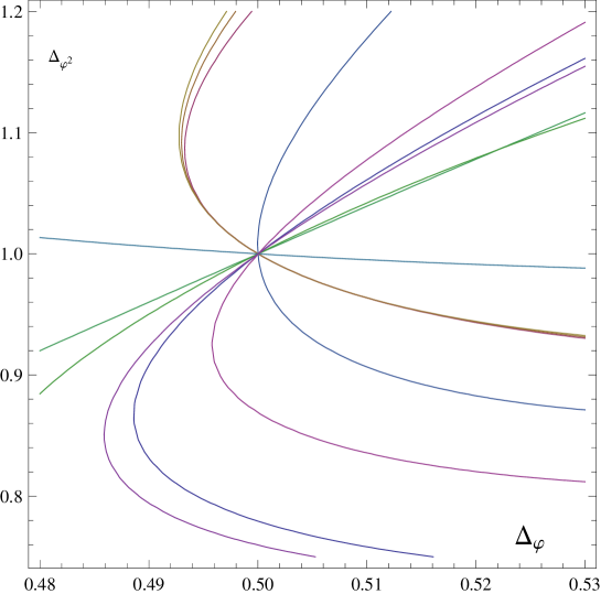
Figure 1: Setting $D=3$ and $\Delta_{4}=\Delta_{\phi^{2}}+2$ in (9) we get a two-dimensional section of the zeros of the 10 $3\times 3$ minors made with the first 5 derivatives specified in the text. The common intersection selects the exact solution of the free field theory.

$$\frac{1}{2}{\sf f}^{(2,0)}_{\Delta_{\phi},\Delta_{\ell}}-\frac{D-1}{3}\,{\sf f}^{(0,1)}_{\Delta_{\phi},\Delta_{\ell}}=0\,;$$ (11)

$$\frac{D(4-D)}{2}\,{\sf f}^{(2,0)}_{\Delta_{\phi},\Delta_{\ell}}-\frac{5}{8}\,{\sf f}^{(4,0)}_{\Delta_{\phi},\Delta_{\ell}}+\frac{(D^{2}-1)}{2}\,{\sf f}^{(0,2)}_{\Delta_{\phi},\Delta_{\ell}}=0\,;$$ (12)

$$3D\,{\sf f}^{(2,0)}_{\Delta_{\phi},\Delta_{\ell}}+(D^{2}-1)\,{\sf f}^{(0,2)}_{\Delta_{\phi},\Delta_{\ell}}-\frac{3(D-1)}{2}\,{\sf f}^{(2,1)}_{\Delta_{\phi},\Delta_{\ell}}=0\,.$$ (13)

Although by construction we would expect that they are only identically satisfied by the conformal blocks retained in the $N=3$ truncation, it turns out, unexpectedly, that the whole infinite set of conformal blocks listed in (8) satisfies them. These surprising identities may be easily verified for the mentioned cases with integer $D$, as for instance (10). For arbitrary $D$ a straightforward check may be obtained by directly applying the above relations to the function $g(u,v)$ defined in (1), which in a free field theory in $D$ dimensions is

$$g(u,v)=1+\left(\frac{u}{v}\right)^{\frac{D-2}{2}}+u^{\frac{D-2}{2}}.$$

It is also easy to check that this solution does not depend on the specific form of the OPE coefficients by replacing $g(u,v)$ with $P(C_{2})\,g(u,v)$, where $P$ is an arbitrary polynomial of the Casimir operator $C_{2}$.

To sum up, we have described an example of truncation that in some sense is exact seeing that it reproduces the true spectrum contributing to a four-point function. There is however a price to be paid. The sum rule (4) tells us that truncating it to a finite number of terms while keeping the true spectrum can not give the exact OPE coefficients. Actually the coefficients obtained solving the truncated equations for $D>3$ differ substantially from the exact values and the solution worsens as $D$ increases. Adding new terms to the truncation does not help very much. In fact, the above identities imply simple zeros for the $3\times 3$ minors, double zeros for the $4\times 4$ minors and so on. In other terms the inhomogeneous system with $N>3$ depends on $N-3$ free parameters and loses part of its predictive power. It is worth noting that the above identities hold true only at the symmetric point $z=\bar{z}=\frac{1}{2}$. In a different point it is no longer possible to reconstruct the true spectrum, the minors do not longer have multiple zeros and for large enough truncations one may obtain reasonable values of the spectrum and OPE couplings.

As an aside, it is instructive to note that equations (11), (12) and (13) are analytic examples of linear functionals whose zeros define the exact spectrum of a whole sector of a CFT. They bear some similarity to the linear functional discussed in [2, 9] in relation with the upper bound set by unitarity. Notice however that our functionals are not positive, with the only exception of eq.(11) in $D=4$ which coincides, up to a suitable change of variables, with the one mentioned in [3], showing that the 4d free field theory belongs to the unitarity upper bound.

Another kind of pathological truncations may be found in 2d CFTs. Here it is known that the identity, the stress tensor as well as an infinite set of operators of known scaling dimension and spin are grouped into a single Virasoro conformal block, therefore part of terms contributing to the sum rule (4) is already known and one might envisage to apply the truncation method to get an approximate evaluation of the unknown part of the spectrum. It turns out that in a sufficiently large truncation all the minors of the homogeneous system (6) made only with $a$ derivatives vanish identically, irrespective of the scaling dimensions and spin of the unknown terms, so they do not provide any information about the unknown part of the spectrum. The explanation of this unexpected behaviour resides in an erratic identity among some terms of the mentioned Virasoro conformal block. Precisely, in the limit $b\to 0$ we have

$$G_{4,0}(u,v)-\frac{3}{700}G_{8,0}(u,v)-\frac{1}{45}G_{6,2}(u,v)-G_{4,4}(u,v)+\frac{25}{6237}G_{8,4}(u,v)=O(b).$$ (14)

Thus all minors containing, besides other entries, only $a$ derivatives of the above five conformal blocks are zero identically. In order to obtain useful information from the homogeneous system (6) we have to always include $b$ derivatives.

3 Encoding bootstrap constraints into polynomial equations

The constraints imposed by conformal symmetry on correlation functions near a boundary were studied in [41] and the boundary bootstrap program was set up in [7].

The study of surface transitions of the 3d Ising and other $O(N)$ models through numerical solutions of truncated bootstrap equations [28] resulted particularly fruitful in the ordinary transition, where the knowledge of the low-lying bulk spectrum allowed to evaluate the scaling dimension of the relevant surface operator which compares well with known results of two-loop calculations [42] and nicely agree with the more precise Monte Carlo estimates [31].

In this Section we show that these equations may be written in a simple algebraic form, thereby enabling an analytic study of the solution.

A CFT in a semi-infinite $D$-dimensional space bounded by a flat $(D-1)$-dimensional boundary is characterized by the spectra of the bulk primary operators associated with representations of the conformal group $SO(D+1,1)$ as well a that of the boundary primaries, associated with representations of $SO(D,1)$. The two point function of identical scalar primaries can be parametrised as

$$\langle\phi(x)\,\phi(x^{\prime})\rangle=\frac{\xi^{-\Delta_{\phi}}}{(4yy^{\prime})^{\Delta_{\phi}}}g(\xi),$$ (15)

where $\xi$ is the invariant combination

$$\xi=\frac{(x-x^{\prime})^{2}}{4yy^{\prime}}.$$ (16)

$x$ denotes a point in the $D$ dimensional space and $y$ its distance from the boundary.

$g(\xi)$ can be expanded either in terms of bulk conformal blocks or in terms of boundary blocks. More precisely we can write

$$g(\xi)=1+\sum_{\cal O}a_{\cal O}\lambda_{\phi\phi{\cal O}}f_{bulk}(\Delta_{\cal O},\xi),$$ (17)

or

$$g(\xi)=\xi^{\Delta_{\phi}}\left(a_{\phi}^{2}+\sum_{\widehat{{\cal O}}}\mu_{\widehat{{\cal O}}}^{2}f_{bdry}(\Delta_{\widehat{{\cal O}}},\xi)\right),$$ (18)

where we denoted the boundary quantities with a hat. Only scalar primaries contribute to both expansions. $\lambda_{\phi\phi{\cal O}}$ is the OPE coefficient already introduced in the four point function (1) and similarly $\mu_{\widehat{{\cal O}}}$ is the bulk-to-surface OPE coefficient; $a_{\cal O}$ parametrises the one point function $\langle{\cal O}(x)\rangle=\frac{a_{\cal O}}{(2y)^{\Delta_{\cal O}}}$. The conformal blocks $f_{bulk}(\Delta,\xi)$ and $f_{bdry}(\Delta,\xi)$ are eigenfunctions of the bulk and the boundary quadratic Casimir operators, namely

$${\cal C}_{2}\,f_{bulk}(\Delta,\xi) =c_{\Delta}f_{bulk}(\Delta,\xi),\leavevmode\nobreak\ c_{\Delta}=\Delta(D-\Delta),$$ (19)

$$\widehat{{\cal C}}_{2}\,f_{bdry}(\Delta,\xi) =b_{\Delta}f_{bdry}(\Delta,\xi),\leavevmode\nobreak\ b_{\Delta}=\Delta(D-1-\Delta).$$ (20)

These conformal blocks are completely fixed once their asymptotic behaviour is given:

$$f_{bulk}(\Delta,\xi)\sim\xi^{\frac{\Delta}{2}}\leavevmode\nobreak\ (\xi\to 0);\leavevmode\nobreak\ \leavevmode\nobreak\ f_{bdry}(\Delta,\xi)\sim\xi^{-\Delta}\leavevmode\nobreak\ (\xi\to\infty).$$ (21)

Later we shall need the explicit form of ${\cal C}_{2}$ and $\widehat{\cal C}_{2}$. They can be easily obtained using the embedding formalism of [39] and [7]

$${\cal C}_{2} =-4\xi^{2}(1+\xi)\frac{d^{2}}{d\xi^{2}}-4\xi(\xi+1-D/2)\frac{d}{d\xi}\leavevmode\nobreak\ ;$$ (22)

$$\widehat{\cal C}_{2} =-\xi(1+\xi)\frac{d^{2}}{d\xi^{2}}-D(\xi+\frac{1}{2})\frac{d}{d\xi}\leavevmode\nobreak\ .$$ (23)

The bootstrap constraint simply expresses the equality of the two above expansions. It can be written again as a sum rule

$$\xi^{\Delta_{\phi}}\left(a_{\phi}^{2}+\sum_{\widehat{{\cal O}}}\mu_{\widehat{{\cal O}}}^{2}f_{bdry}(\Delta_{\widehat{{\cal O}}},\xi)\right)-\sum_{\cal O}a_{\cal O}\lambda_{\phi\phi{\cal O}}f_{bulk}(\Delta_{\cal O},\xi)=1.$$ (24)

We want now apply such a constraint to the study of surface transitions in $D=3$. First, we rewrite this functional equation in the form of infinitely many linear equations, one for each coefficient of the Taylor expansion around, say, $\xi=1$. Then, we truncate the two sums keeping only $n_{bulk}$ terms in the bulk channel and $n_{bdry}$ terms in the boundary channel. We also truncate the Taylor expansion by keeping a finite number $M$ of derivatives. We denote this truncation by the triple $(n_{bulk},n_{bdry},s)$, where $s=1$ if the considered surface transition allows $a_{\phi}\not=0$, otherwise we set $s=0$. Using obvious shorthand notations, the truncated system may be written in the form

$$a^{2}_{\phi}+\sum_{i}^{n_{bdry}}{\sf q}_{i}\,f_{bdry}(\Delta_{i},\xi=1)-\sum_{k}^{n_{bulk}}{\sf p}_{k}\,f_{bulk}(\Delta_{k},\xi=1)=1,\leavevmode\nobreak\ \leavevmode\nobreak\ \leavevmode\nobreak\ \leavevmode\nobreak\ n_{bulk}+n_{bdry}+s=N$$ (25)

$$\partial_{\xi}^{n}\left[\xi^{\Delta_{\phi}}\left(a^{2}_{\phi}+\sum_{i}^{n_{bdry}}{\sf q}_{i}\,f_{bdry}(\Delta_{i},\xi)\right)-\sum_{k}^{n_{bulk}}{\sf p}_{k}\,f_{bulk}(\Delta_{k},\xi)\right]_{|_{\xi=1}}=0.\leavevmode\nobreak\ \leavevmode\nobreak\ n=1.\dots,M$$ (26)

This truncation becomes predictive if one can find solutions of the homogeneous system (26) with $M\geq N$. Interesting solutions have been found for $M=N+1$ or $M=N+2$, while truncations with $M>N+2$ do not yield reliable solutions [28].

The simplest solution analyzed in [28] is associated with the truncation $(2,1,0)$. It has been shown to give the scaling dimension of the relevant surface operator of the ordinary transition in terms of the scaling dimensions of $\phi,\epsilon$ and $\epsilon^{\prime}$, where $\phi$ is the fundamental scalar,$\epsilon$ the energy operator, and $\epsilon^{\prime}$ its first recurrence (related to the correction-to-scaling exponent $\omega$) of the 3d $O(N)$ theory.

We want to rewrite this solution in an algebraic form. First, note that the Casimir operators (22) and (23) enable us to write the $n^{\rm th}$ derivative of the bulk or boundary conformal blocks as a linear combination of the conformal block and its first derivative

$$\frac{d^{n}}{d\xi^{n}}f_{bulk}={\sf P}_{n}(c)f_{bulk}+{\sf Q}_{n-1}(c)f_{bulk}^{\prime};\leavevmode\nobreak\ \frac{d^{n}}{d\xi^{n}}f_{bdry}=\widehat{\sf P}_{n}(b)f_{bdry}+\widehat{\sf Q}_{n-1}(b)f_{bdry}^{\prime},$$ (27)

where ${\sf P}_{n},{\sf Q}_{n},\widehat{\sf P}_{n}$ and $\widehat{\sf Q}_{n}$ are polynomials of degree $[\frac{n}{2}]$ on their argument.

In $D=3$ $f_{bdry}(\Delta,\xi)$ can be expressed as elementary algebraic functions [28], namely

$$f_{bdry}(\Delta,\xi)=\frac{1}{2\sqrt{\xi}}\left(\frac{4}{1+\xi}\right)^{\Delta-\frac{1}{2}}\left[1+\sqrt{\frac{\xi}{1+\xi}}\right]^{-2(\Delta-1)}.$$ (28)

It will entail a dramatic simplification of the bootstrap equations. We only need to take advantage of the following two identities

$$z\equiv\frac{f_{bdry}^{\prime}(\Delta,\xi)|_{\xi\to 1}}{f_{bdry}(\Delta,1)}=-\frac{3-2(1-\Delta)\sqrt{2}}{4};\leavevmode\nobreak\ b\equiv(2-\Delta)\Delta=-\frac{1}{8}-3z-2z^{2},$$ (29)

to express $\frac{d^{n}}{d\xi^{n}}f_{bdry}$ as a polynomial in $\Delta$ (or in $z$). As a consequence, the homogeneous system (26) associated with the (2,1,0) truncation can be written as

$$x\,{\sf p}_{\epsilon}{\sf Q}_{n-1}(c_{\epsilon})+y\,{\sf p}_{\epsilon^{\prime}}{\sf Q}_{n-1}(c_{\epsilon^{\prime}})+{\sf p}_{\epsilon}{\sf P}_{n}(c_{\epsilon})+{\sf p}_{\epsilon^{\prime}}{\sf P}_{n}(c_{\epsilon^{\prime}})={\sf q}{\cal P}_{n}(\Delta_{\phi},\Delta),$$ (30)

where ${\cal P}_{n}$ is a polynomial of degree $n$ in its arguments and we set

$$x\equiv\frac{f_{bulk}^{\prime}(\Delta_{\epsilon},\xi)|_{\xi\to 1}}{f_{bulk}(\Delta_{\epsilon},1)},\,y\equiv\frac{f_{bulk}^{\prime}(\Delta_{\epsilon^{\prime}},\xi)|_{\xi\to 1}}{f_{bulk}(\Delta_{\epsilon^{\prime}},1)}.$$ (31)

We can even eliminate $x$ and $y$ in (30) by combining the derivatives in such a way to form a power of ${\cal C}_{2}$, so to have

$${\sf p}_{\epsilon}\,c_{\epsilon}^{m}+{\sf p}_{\epsilon^{\prime}}\,c_{\epsilon^{\prime}}^{m}={\sf q}\,{\cal Q}_{2m}(\Delta_{\phi},\Delta),$$ (32)

where ${\cal Q}_{2m}$ is another polynomial of degree $2m$ in its arguments.

In order to find a solution of the (2,1,0) truncation we have to choose three equations among the two sets (30) and (32), with the constraint that the order of the maximal derivative acting on $f_{bulk}$ and $f_{bdry}$ should not exceed $n_{bulk}+n_{bdry}+s+2=5$, therefore one equation, at least, should be of the type (30). We pick two equations of type (32) with $m=1,2$ and one of type (30) with $n<5$. In this way we can form four different subsystems of three equations in three unknowns. Note that the associated minors are linear in $x$ and $y$. Taking any two of them we can solve for $x$ and $y$. Remarkably, the solution does not depend on the pair chosen. We have

$$\frac{2}{c_{\epsilon}}x\equiv\frac{2f_{bulk}^{\prime}(\Delta_{\epsilon},\xi)|_{\xi\to 1}}{c_{\epsilon}\,f_{bulk}(\Delta_{\epsilon},1)}=\frac{{\sf A}(c_{\epsilon^{\prime}},\Delta_{\phi},z)}{{\sf B}(c_{\epsilon^{\prime}},\Delta_{\phi},z)}\,,$$ (33)

with

$${\sf A}\left(c,\frac{f}{4},z\right)=4-(3+2c)f+f^{2}-f^{3}-(1+2c+f+3f^{2})4z-(2+3f)(4z)^{2}-(4z)^{3}$$ (34)

and

$${\sf B}\left(c,\frac{f}{4},z\right)= 21+2c-6(3+c)f+(17+2c)f^{2}-2f^{3}+f^{4}-16(1+c-(6+c)f-f^{3})z$$

$$+ 2(5+c+3f+3f^{2})(4z)^{2}+4(1+f)(4z)^{3}+(4z)^{4}.$$ (35)

Clearly the above relation defines an algebraic equation of degree four in $\Delta$, hence it can be solved exactly. Replacing the bulk quantities $\Delta_{\phi},\Delta_{\epsilon},\Delta_{\epsilon^{\prime}}$ with the known values of the 3d $O(N)$ models one gets at once an estimate of the scaling dimension of the relevant surface operator of the ordinary transition, which is almost identical with that obtained in [28] using numerical means.

Being Eq. (33) a quartic equation, it has other three roots. In the 3d Ising model one is at $\Delta\simeq 3.08$ (it could have some to do with the extraordinary transition, where $\Delta=3$ exactly, however it requires $a_{\phi}\not=0$ and is described by the truncation (2,1,1)). The other two are complex conjugate with a real part $\Re e(\Delta)\simeq 0.35$, close to the expected value of the leading critical exponent of the special transition. One has to add more terms to the truncation in order to describe a full-fledged special transition.

Besides eq.(33) there is another similar equation generated by the present analytical method. It suffices to exchange $\epsilon\leftrightarrow\epsilon^{\prime}$ in (33). The estimate of $\Delta$ obtained this way is slightly shifted. Again, in order to reduce the spread between these two estimates one may try to find more accurate solutions by adding new bulk and/or boundary terms to the truncation, however this addition transforms the isolated solution discussed in this section into a one-parameter family of solutions. This issue will be discussed in the next section.

4 Ordinary versus special transition

The algebraic method described in the previous Section does not apply to other viable truncations, as it requires in general too high derivatives. For example, the (4,1,1) truncation utilized in [28] to describe the extraordinary transition would require 10 derivatives at least. A similar conclusion applies to the one-parameter family of solutions of (3,3,0) or (4,3,0) studied in [28], or of (4,4,0) analyzed here, in relation with the special transition. Nevertheless in the latter case the peculiar algebraic properties of $f_{bdry}$ will help us to clarify some features of this kind of truncation. Eventually, it will lead to a precise estimate of the scaling dimensions of the relevant surface operators in both special and ordinary transitions.

Notice that one-parameter solutions of truncated bootstrap equations were also encountered in the study of four-point functions [27], however in that case the choice of the low-lying bulk spectrum fixed uniquely the value of the free parameter, while in the case of boundary CFTs the knowledge of the bulk spectrum does no longer suffice to fix the surface spectrum.

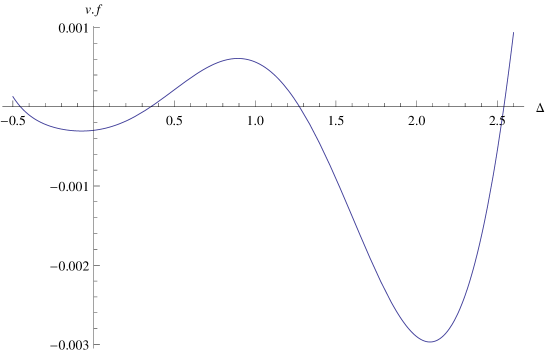
Figure 2: The scalar product ${\sf v}\cdot f$ of a null left eigenvector of the $8\times 8$ minor ${\sf f}$ associated with the truncation (4,4,0) as a function of the scaling dimension of the surface operators.$f$ is the column vector defined in eq.(37). Notice that ${\sf v}\cdot{f}$ is a polynomial of $8^{\rm th}$ degree in $\Delta$, so it has more zeros than the four values that form a solution of (4,4,0). The additional zeros may be employed to form other solutions.

As already explained in the Introduction, a physical motivation of such a behaviour may be found in the fact that the boundary bootstrap equations coincide with interface bootstrap equations, where the conformal interface is the domain wall between the critical Ising model and another CFT. The main difference between a simple boundary or a more general conformal interface of 3d Ising model resides in the boundary conditions, which are necessarily Dirichlet or Neumann in the former and more general in the latter. The case where there is a free field theory in one side of the interface has been analytically worked out in [28]. It turns out that its boundary conditions depend on a free parameter interpolating continuously between Dirichlet an Neumann conditions.

Likewise the free parameter of the mentioned solutions is presumably a direct consequence of these more general boundary conditions. This is also supported by the fact that the solutions of the different truncations (3,3,0), (4,3,0) and (4,4,0) depend always on a single parameter, though they deal with different numbers of unknowns. Thus the problem of estimating the low-lying surface operators in the special transition can be reformulated, within this way of reasoning, in that of finding the value of the free parameter corresponding to the Neumann conditions (the boundary conditions characterizing the special transition in the $\phi^{4}$ field theory).

There is another element to be taken into account. Notice that the bootstrap equations of the special transition are the same of those describing the ordinary transition. The solution is different, as the latter corresponds to Dirichlet boundary conditions. Therefore it should exist another value of the free parameter of the solution of, say, (4,4,0), describing also such a surface transition.

The numerical approach to solve truncated bootstrap equations is based on the Newton method, which requires as input a starting point with an approximate guess of the solution, thus it is not suitable for an exhaustive search. Here we describe a way out which takes advantage of the algebraic properties of the boundary conformal blocks.

In any CFT on a manifold with a boundary there is a short distance expansion expressing local bulk operators in terms of boundary operators. In the case of special transition of the critical 3d Ising model we have the fusion rule

$$\sigma\sim\widehat{\sigma}+\widehat{{\cal O}}_{s}+\dots$$ (36)

where $\sigma$ is the lowest scalar in the bulk, $\widehat{\sigma}$ the corresponding surface operator and $\widehat{{\cal O}}_{s}$ the next-to-leading surface primary. Applying the direct numerical method of [28] to (3,4,0) or (4,4,0) truncations one may verify that unitary solutions exist only for $0.3\leq\Delta_{\widehat{\sigma}}\leq 0.45$ and $2\leq\Delta_{\widehat{{\cal O}}_{s}}\leq 2.6$. We have two other surface operators whose role is to provide more stable solutions.

Every solution defines a left null eigenvector ${\sf v}$ of the $8\times 8$ matrix ${\sf f}$ of the homogeneous system $(\ref{bhomo})$ such that ${\sf v\,f}=0$. Define now the vector

$$f(\Delta)=(\partial_{\xi}\,\,\xi^{\Delta_{\sigma}}f_{bdry},\partial^{2}_{\xi}\,\,\xi^{\Delta_{\sigma}}f_{bdry},\dots,\partial^{8}_{\xi}\,\,\xi^{\Delta_{\sigma}}f_{bdry}),$$ (37)

which is a column of ${\sf f}$. According to (27), the scalar product ${\sf v\cdot}f$ is a polynomial of $8^{\rm th}$ degree in $\Delta$, therefore it vanishes not only at the four points of the chosen solution, but also at other four values (some of them are plotted in Figure 2). Actually every subset of four roots of this polynomial defines a solution. Most of them are uninteresting as they reveal some non-unitary features. There is however a solution which is physically interesting. Its fusion rule in the boundary channel can be written as

$$\sigma\sim\frac{d{\widehat{\sigma}}}{dy}+(\widehat{{\cal O}}_{s})+\widehat{{\cal O}}_{o}+\dots$$ (38)

where the lowest surface operator is identified with the one of the ordinary transition since it has similar scaling dimensions and similar OPE coefficients of the solution found in the previous Section.

The term $\widehat{{\cal O}}_{s}$ coincides with that of (36). We put it within parentheses seeing that its square coupling $\mu^{2}_{\widehat{{\cal O}}_{s}}$ changes sign as we scan the family of solutions.

Actually the point where $\mu^{2}_{\widehat{{\cal O}}_{s}}=0$, corresponding to the fusion rule $\sigma\sim\frac{d{\widehat{\sigma}}}{dy}+\widehat{{\cal O}}_{o}+\dots$, selects the sought after solution, as it can be argued putting together the following three statements:

• According to the fusion rule (36), $\widehat{{\cal O}}_{s}$ is non-vanishing on surfaces with Neumann boundary conditions, seeing that it is always present whenever $\widehat{\sigma}$ is there.

• There is no reason to believe that an operator contributing to a surface transition with, say, Neumann boundary conditions could survive, with the same scaling dimension, on a surface with Dirichlet boundary conditions.

• The fusion rule (38) with $\mu^{2}_{\widehat{{\cal O}}_{s}}=0$ is the only solution compatible with Dirichlet boundary conditions. The corresponding value of $\Delta_{{\cal O}_{s}}$ is the only one compatible with pure Neumann boundary conditions in (36).

In conclusion, we have selected in the one-parameter family for Ising conformal interfaces a pair of solutions describing the special and the ordinary transition.

5 Numerical results and concluding remarks

In the previous Section we described a method to get numerical estimates of the low-lying spectrum of surface operators in ordinary and special transitions of 3d Ising universality class in terms of the bulk spectrum. In table 1 we report the most significant quantities generated by the (4,4,0) truncation.

The input parameters are the scaling dimensions of the bulk operators $\sigma,\epsilon,\epsilon^{\prime},\epsilon^{\prime\prime}$ and $\epsilon^{\prime\prime\prime}$, namely,

$$\Delta_{\sigma}=0.5181489(10);\leavevmode\nobreak\ \Delta_{\epsilon}=1.412625(10),$$

taken from [25], $\Delta_{\epsilon}=3.8303(18)$ taken from [11], and $\Delta_{\epsilon^{\prime\prime}}=7.316(14);\leavevmode\nobreak\ \Delta_{\epsilon^{\prime\prime\prime}}=13.05(4)$ from the truncation (4,1,1) studied in [28].

Ordinary surface transition in 3d Ising bulk universality class
Ref	year	method	$y_{h}=2-\Delta_{\frac{d{\widehat{\sigma}}}{dy}}$	$\Delta_{{\cal O}_{o}}$
[43]	$1981$	$\varepsilon-\textup{expansion}$	$0.762$
[42]	$1998$	3d two-loop exp.	$0.714$
[46]	$2005$	Monte Carlo	$0.7374(15)$
[31]	$2011$	Monte Carlo	$0.7249(6)$
[28]	$2015$	Bootstrap	$0.724(2)$
this work	$2016$	Bootstrap	$0.72558(18)$	$5.13(20)$

Special surface transition in 3d Ising bulk universality class
Ref	year	method	$y_{h}=2-\Delta_{\widehat{\sigma}}$	$y_{t}$	$\Delta_{{\cal O}_{s}}$
[44, 45]	$1983$	$\varepsilon-\textup{expansion}$	$1.65$	$1.08$
[42]	$1998$	3d two-loop exp.	$1.583$	$0.856$
[46]	$2005$	Monte Carlo	$1.636(91)$	$0.715(1)$
[38]	$2011$	Monte Carlo	$1.6465(6)$	$0.718(2)$
[28]	$2015$	Bootstrap	$1.55\div 1.7$		$2\div 2.6$
this work	$2016$	Bootstrap	$1.6460(20)$		$2.54(2)$

Surface transition	$a_{\varepsilon}\lambda_{\sigma\sigma\varepsilon}$	$a_{\varepsilon^{\prime}}\lambda_{\sigma\sigma\varepsilon^{\prime}}$	$\mu_{1}^{2}$	$\mu_{2}^{2}$
Ordinary	$-0.7862(2)$	$0.0413(1)$	$0.7560(1)$	$0.000049(6)$
Special	$1.216(13)$	$0.081(3)$	$2.06(1)$	$0.0251(7)$

Table 1: In the first two tables we compare our results with those obtained by field theoretic methods and Monte Carlo studies. The last table collects the most relevant OPE coefficients. In the ordinary transition $\mu_{1}=\mu_{\frac{d\widehat{\sigma}}{dy}}$ and $\mu_{2}=\mu_{\widehat{{\cal O}}_{o}}$, while in the special transition $\mu_{1}=\mu_{\widehat{\sigma}}$ and $\mu_{2}=\mu_{\widehat{{\cal O}}_{s}}$. The first three OPE coefficients in the ordinary transition agree with those computed in [28].

In the first two tables we compare our results for the relevant surface exponents of the two transitions with those obtained with perturbative expansions in $\phi^{4}$ field theory or computed in Monte Carlo simulations. Following the literature, here we replaced the scaling dimension $\Delta$ with the surface renormalization group exponent $y_{h}=2-\Delta$. The field-theoretic approach to critical behaviour near free surfaces is rather challenging, mainly because the breakdown of translational invariance gives rise to serious computational difficulties. As a matter of fact expansions in 4-$\varepsilon$ dimensions [43, 44, 45] or 3d expansions in a massive model[42] do not exceed second order. Better results are obtained with Monte Carlo simulations [46, 31, 38].

The error in our bootstrap results is due to the uncertainty of the input parameters. The major sources of error are the uncertainties of the scaling dimensions of $\epsilon^{\prime\prime}$ and $\epsilon^{\prime\prime\prime}$, while the errors and the central values do not vary sensibly when we replace the values of $\Delta_{\sigma}$ and $\Delta_{\epsilon}$ with the estimates obtained in Monte Carlo simulations [47].

The method described in this work, being based on the interplay between ordinary and special transition, can not be directly generalized to $O(N)$ models with $N>1$. In fact the special transition is an order-disorder transition on the surface boundary, while there can not be any spontaneous breaking of a continuous symmetry in $D\leq 2$ dimensions, according to the Mermin-Wagner-Hohenberg theorem. Actually the special transition, being multicritical, is characterized by two relevant renormalization group exponents, the magnetic ($y_{h}$) and the thermal ($y_{t}$) exponents. The latter is related to the fusion rule of the bulk energy in the boundary channel $\epsilon\sim 1+\widehat{\epsilon}+\dots$ by $y_{t}=2-\Delta_{\widehat{\epsilon}}$. For completeness some values of $y_{t}$ are reported in the second table. So far, no suitable solution of the bootstrap equations has been found to compute $\Delta_{\widehat{\epsilon}}$. The algebraic formalism developed in this paper could help to face this problem.

References

- [1] S. Ferrara, A. Grillo, and R. Gatto, Tensor representations of conformal algebra and conformally covariant operator product expansion, Annals Phys. 76 (1973) 161–188.
- [2] R. Rattazzi, V. S. Rychkov, E. Tonni, and A. Vichi, Bounding scalar operator dimensions in 4D CFT, JHEP 0812 (2008) 031, arXiv:0807.0004 [hep-th].
- [3] V. S. Rychkov and A. Vichi, Universal Constraints on Conformal Operator Dimensions, Phys.Rev. D80 (2009) 045006, arXiv:0905.2211 [hep-th].
- [4] R. Rattazzi, S. Rychkov, and A. Vichi, Central Charge Bounds in 4D Conformal Field Theory, Phys.Rev. D83 (2011) 046011, arXiv:1009.2725 [hep-th].
- [5] D. Poland and D. Simmons-Duffin, Bounds on 4D Conformal and Superconformal Field Theories, JHEP 1105 (2011) 017, arXiv:1009.2087 [hep-th].
- [6] S. El-Showk, M. F. Paulos, D. Poland, S. Rychkov, D. Simmons-Duffin, A. Vichi, Solving the 3D Ising Model with the Conformal Bootstrap, Phys.Rev. D86 (2012) 025022, arXiv:1203.6064 [hep-th].
- [7] P. Liendo, L. Rastelli, and B. C. van Rees, The Bootstrap Program for Boundary , JHEP 1307 (2013) 113, arXiv:1210.4258 [hep-th].
- [8] D. Pappadopulo, S. Rychkov, J. Espin, and R. Rattazzi, OPE Convergence in Conformal Field Theory, Phys.Rev. D86 (2012) 105043, arXiv:1208.6449 [hep-th].
- [9] S. El-Showk and M. F. Paulos, Bootstrapping Conformal Field Theories with the Extremal Functional Method, Phys.Rev.Lett. 111 (2013) no.~24, 241601, arXiv:1211.2810 [hep-th].
- [10] D. Gaiotto, D. Mazac, and M. F. Paulos, Bootstrapping the 3d Ising twist defect, JHEP 1403 (2014) 100, arXiv:1310.5078 [hep-th].
- [11] S. El-Showk, M. F. Paulos, D. Poland, S. Rychkov, D. Simmons-Duffin, and A. Vichi, Solving the 3d Ising Model with the Conformal Bootstrap II. c-Minimization and Precise Critical Exponents, J. Stat. Phys. 157 (2014) 869, arXiv:1403.4545 [hep-th].
- [12] C. Beem, L. Rastelli, and B. C. van Rees, The Superconformal Bootstrap, Phys.Rev.Lett. 111 (2013) 071601, arXiv:1304.1803 [hep-th].
- [13] Y. Nakayama and T. Ohtsuki, Five dimensional -symmetric CFTs from conformal bootstrap, Phys.Lett. B734 (2014) 193–197, arXiv:1404.5201 [hep-th].
- [14] Y. Nakayama and T. Ohtsuki, Bootstrapping phase transitions in QCD and frustrated spin systems, Phys. Rev. D91 (2015) no.~2, 021901, arXiv:1407.6195 [hep-th].
- [15] S. M. Chester, J. Lee, S. S. Pufu, and R. Yacoby, The superconformal bootstrap in three dimensions, JHEP 1409 (2014) 143, arXiv:1406.4814 [hep-th].
- [16] F. Kos, D. Poland, and D. Simmons-Duffin, Bootstrapping Mixed Correlators in the 3D Ising Model, JHEP 11 (2014) 109, arXiv:1406.4858 [hep-th].
- [17] S. M. Chester, S. S. Pufu, and R. Yacoby, Bootstrapping O(N) Vector Models in 4 < d < 6, arXiv:1412.7746 [hep-th].
- [18] C. Beem, M. Lemos, P. Liendo, L. Rastelli, and B. C. van Rees, The superconformal bootstrap, JHEP 03 (2016) 183, arXiv:1412.7541 [hep-th].
- [19] D. Simmons-Duffin, A Semidefinite Program Solver for the Conformal Bootstrap, JHEP 06 (2015) 174, arXiv:1502.02033 [hep-th].
- [20] N. Bobev, S. El-Showk, D. Mazac, and M. F. Paulos, Bootstrapping the Three-Dimensional Supersymmetric Ising Model, Phys. Rev. Lett. 115 (2015) no.~5, 051601, arXiv:1502.04124 [hep-th].
- [21] F. Kos, D. Poland, D. Simmons-Duffin, and A. Vichi, Bootstrapping the O(N) Archipelago, JHEP 11 (2015) 106, arXiv:1504.07997 [hep-th].
- [22] N. Bobev, S. El-Showk, D. Mazac, and M. F. Paulos, Bootstrapping SCFTs with Four Supercharges, JHEP 08 (2015) 142, arXiv:1503.02081 [hep-th].
- [23] C. Beem, M. Lemos, L. Rastelli, and B. C. van Rees, The (2, 0) superconformal bootstrap, Phys. Rev. D93 (2016) no.~2, 025016, arXiv:1507.05637 [hep-th].
- [24] Y. Nakayama and T. Ohtsuki, Conformal Bootstrap Dashing Hopes of Emergent Symmetry, arXiv:1602.07295 [cond-mat.str-el].
- [25] F. Kos, D. Poland, D. Simmons-Duffin, and A. Vichi, Precision Islands in the Ising and Models, arXiv:1603.04436 [hep-th].
- [26] F. Gliozzi, More constraining conformal bootstrap, Phys.Rev.Lett. 111 (2013) 161602, arXiv:1307.3111.
- [27] F. Gliozzi and A. Rago, Critical exponents of the 3d Ising and related models from Conformal Bootstrap, JHEP 1410 (2014) 42, arXiv:1403.6003 [hep-th].
- [28] F. Gliozzi, P. Liendo, M. Meineri, and A. Rago, Boundary and Interface CFTs from the Conformal Bootstrap, JHEP 05 (2015) 036, arXiv:1502.07217 [hep-th].
- [29] S. Rychkov and P. Yvernay, Remarks on the Convergence Properties of the Conformal Block Expansion, Phys. Lett. B753 (2016) 682–686, arXiv:1510.08486 [hep-th].
- [30] J. A. Gracey, Four loop renormalization of theory in six dimensions, Phys. Rev. D92 (2015) no.~2, 025012, arXiv:1506.03357 [hep-th].
- [31] M. Hasenbusch, The thermodynamic Casimir force: A Monte Carlo study of the crossover between the ordinary and the normal surface universality class, Phys.Rev. B 83 (2011) 134425, arXiv:1012.4986.
- [32] Y. Nakayama, Bootstrapping critical Ising model on three-dimensional real projective space, Phys. Rev. Lett. 116 (2016) 141602, arXiv:1601.06851 [hep-th].
- [33] T. Quella, I. Runkel and G. M. T. Watts, Reflection and transmission for conformal defects, JHEP 0704 (2007) 095, arXiv:hep-th/0611296.
- [34] M. Billò, V. Goncalves, E. Lauria and M. Meineri, Defects in conformal field theory, JHEP 1604 (2016) 091 doi:10.1007/JHEP04(2016)091 arXiv:1601.02883 [hep-th].
- [35] R. Abe, d’ Dimensional Defect in d-Dimensional Lattice. I Nonuniversal Local Critical Exponent in the Limit , Prog. Theor. Phys. 65, 1237 (1981).
- [36] B. M. McCoy and J. H. H. Perk, Two Spin Correlation Functions of an Ising Model With Continuous Exponents, Phys. Rev. Lett. 44 (1980) 840.
- [37] M. Oshikawa and I. Affleck, Boundary conformal field theory approach to the critical two-dimensional Ising model with a defect line, Nucl. Phys. B495 (1997) 533–582, arXiv:cond-mat/9612187 [cond-mat].
- [38] M. Hasenbusch, Monte Carlo study of surface critical phenomena: The special point,Phys. Rev. B 84 (Oct, 2011) 134405, arXiv:1108.2425.
- [39] F. Dolan and H. Osborn, Conformal partial waves and the operator product expansion, Nucl.Phys. B678 (2004) 491–507, arXiv:hep-th/0309180 [hep-th].
- [40] S. Weinberg, Minimal fields of canonical dimensionality are free, Phys. Rev. D86 (2012) 105015, arXiv:1210.3864 [hep-th].
- [41] D. McAvity and H. Osborn, Conformal field theories near a boundary in general dimensions, Nucl.Phys. B455 (1995) 522–576, arXiv:cond-mat/9505127 [cond-mat].
- [42] H. Diehl and M. Shpot, Massive field theory approach to surface critical behavior in three-dimensional systems, Nucl.Phys. B528 (1998) 595–647, arXiv:cond-mat/9804083 [cond-mat].
- [43] H. W. Diehl and S. Dietrich, Field-theoretical approach to static critical phenomena in semi-infinite systems, Zeit. Phys. B42 (1981) 65–86.
- [44] H. Diehl and S. Dietrich, Field-theoretical approach to multicritical behavior near free surfaces, Phys.Rev. B24 (1981) 2878–2880.
- [45] H. Diehl and S. Dietrich, Multicritical behaviour at surfaces, Zeit. f. Phys B 50 (1983) 117.
- [46] Y. J. Deng, H. W. J. Blöte, and M. P. Nightingale, Surface and bulk transitions in three-dimensional O(n) models, Phys. Rev. E72 (2005) 016128–016138, arXiv:cond-mat/0504173.
- [47] M. Hasenbusch, Finite size scaling study of lattice models in the three-dimensional Ising universality class, Phys.Rev. B82 (2010) 174433, arXiv:1004.4486.