Simultaneous Measurement of Complementary Observables with Compressive Sensing

Abstract

The more information a measurement provides about a quantum system’s position statistics, the less information a subsequent measurement can provide about the system’s momentum statistics. This information trade-off is embodied in the entropic formulation of the uncertainty principle. Traditionally, uncertainty relations correspond to resolution limits; increasing a detector’s position sensitivity decreases its momentum sensitivity and vice-versa. However, this is not required in general; for example, position information can instead be extracted at the cost of noise in momentum. Using random, partial projections in position followed by strong measurements in momentum, we efficiently determine the transverse-position and transverse-momentum distributions of an unknown optical field with a single set of measurements. The momentum distribution is directly imaged, while the position distribution is recovered using compressive sensing. At no point do we violate uncertainty relations; rather, we economize the use of information we obtain.

Measurements on quantum systems are always constrained by uncertainty relations. Localizing a particle in one observable, such as position, imparts a disturbance that makes a following measurement of a complementary observable, such as momentum, unpredictable. Such strong, projective measurements are often said to “collapse” the quantum wavefunction. For example, in Young’s double slit experiment, it is not possible to detect through which slit particles pass (position) while also observing interference fringes in the far field (momentum) Bohr (1928).

Consequently, the statistics of complementary observables are usually measured separately; an ensemble of identically prepared particles is directed to a position detector and a different, similarly prepared ensemble is directed to a momentum detector. If a detector instead measures both observables simultaneously with strong measurements, its position resolution $\Delta_{x}$ and momentum resolution $\Delta_{k}$ are bounded by Heisenberg’s uncertainty relation, $\Delta_{x}\Delta_{k}\geq 1/2$. In its most basic form, a Shack-Hartmann wavefront sensor is an example of this kind of detector Platt et al. (2001).

Though this resolution limitation applies to strong measurements, it is not true in general. Here, the uncertainty principle implies an information exclusion principle Maassen and Uffink (1988); Hall (1995); the more information a detector gives about position, the less information it can provide about momentum and vice-versa. With a single, carefully designed experiment, one can simultaneously recover the statistics of both observables at arbitrary resolution. This has been demonstrated, albeit very inefficiently, with weak measurement Lundeen et al. (2011); Kocsis et al. (2011); Dressel et al. (2013).

Figure 1: Experimental setup for simultaneous position and momentum imaging. A state is prepared by illuminating an object mask at $z=z_{0}$ with a plane wave from an attenuated, HeNe laser. The field is imaged at $z=z_{x}$ where it is sequentially filtered by a series of $M$, $256\times 256$ pixel, random, binary filters $\bm{F_{i}}$. Each filter partially projects the state by blocking about half of the position elements. A cooled CCD array in the focal plane $z=z_{k}$ of a Fourier transforming lens records the momentum distribution for each filtered state. Position information is mapped to the total optical power passing each filter; this measures the correlation between the position intensity distribution at $z_{x}$ with the current filter. Because the filters do not strongly localize the photons’ position, the momentum distribution is directly recovered by averaging the CCD images. The position distribution is reconstructed using compressive sensing techniques such that an $N$-pixel position image requires $M<<N$ filters.

In this Letter, we efficiently obtain the transverse-position and transverse-momentum distributions of optical photons from a single set of measurements at high resolution. We sequentially perform a series of random, partial projections in position followed by strong projective measurements of the momentum. The partial projections efficiently extract information about the photons’ position distribution at the cost of injecting a small amount of noise into their momentum distribution. This allows the momentum distribution to be directly observed on a charge-coupled device (CCD) camera. The position distribution is recovered using a computational technique called compressive sensing (CS) Donoho (2006).

Consider an optical field at plane $z=z_{0}$ with transverse, complex amplitude $\psi(\vec{x})$, where $z$ is the propogation direction and $\vec{x}=(x,y)$ are transverse, spatial coordinates. The field also has momentum amplitude $\psi(\vec{k})$ which is related to $\psi(\vec{x})$ by a Fourier transform, with $\vec{k}=(k_{x},k_{y})$.

To measure the position field intensity $|\psi(\vec{x})|^{2}$, one could raster scan a small pinhole through the transverse plane at $z=z_{0}$. The fractional power passing through the pinhole as a function of its position reveals the image. From a quantum perspective, this process constitutes a strong projective position measurement; the pinhole localizes the position of photons passing through it and their subsequent momenta are random. From a classical optics perspective, the pinhole acts like a spatial filter; light passing through the pinhole diffracts evenly in all directions. In either case, information about the original field’s momentum $\psi(\vec{k})$ is lost. Note that one could instead choose to measure the momentum distribution $|\psi(\vec{k})|^{2}$ by performing a similar scan in the focal plane of a Fourier transforming lens. Here, position information would instead be forfeit.

In our approach (Fig. 1), we perform a series of partially projective measurements of position followed by strong measurements of momentum. We first prepare a transverse, photonic state $\psi(\vec{x})$ by illuminating an object mask with a collimated laser. We image this field at plane $z=z_{x}$ with a 4F imaging system. Here we sequentially perform partial projections of $\psi(\vec{x})$ by filtering it with a series of $M$ binary amplitude masks $f_{i}(\vec{x})$. Each mask consists of a random, $N$-pixel pattern, where each pixel either fully transmits or fully obstructs with equal probability. Note that the total optical power passing the $i^{\text{th}}$ filter gives the correlation between that filter and the position intensity distribution $|\psi(\vec{x})|^{2}$. In this way, a small amount of information about the position distribution is extracted without localizing the field. The filtered state $\tilde{\psi}_{i}(\vec{x})=\psi(\vec{x})f_{i}(\vec{x})$ then passes through a Fourier transforming lens to a CCD array in the lens’ focal plane at $z=z_{k}$. The CCD records $M$ images of the momentum distribution of the filtered field $|\tilde{\psi}_{i}(\vec{k})|^{2}$, one for each filter. This set of images contains information about both $\psi$’s position and momentum.

The momentum distribution $|\tilde{\psi}(\vec{k})|^{2}$ is recovered directly from the CCD images by simple averaging such that

$$|\psi(\vec{k})|^{2}=\langle|\tilde{\psi}_{i}(\vec{k})|^{2}\rangle,$$ (1)

where angled brackets indicate an average over all filters. This is made possible by the surprising fact that $|\tilde{\psi}_{i}(\vec{k})|^{2}$ is a good approximation to $|\psi(\vec{k})|^{2}$, even though $|\tilde{\psi}_{i}(\vec{x})|^{2}$ is missing half of its coefficients.

By the convolution theorem of Fourier optics Goodman (2005), the filtered $i^{\text{th}}$ momentum distribution is found by convolving the Fourier transforms of $\psi(\vec{x})$ and $f_{i}(\vec{x})$ such that

$$|\tilde{\psi}_{i}(\vec{k})|^{2}=|\psi(\vec{k})\ast f_{i}(\vec{k})|^{2},$$ (2)

where $\ast$ denotes convolution. To understand the filter’s effect on $\psi(\vec{k})$, we must consider its Fourier transform (Fig. 2).

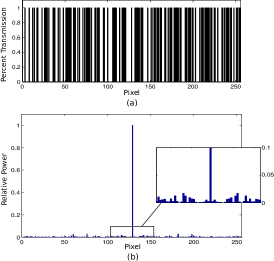
Figure 2: Discrete Fourier transform of a 256 pixel, 1D random, binary pattern. (a) gives a random, binary 1D filter function where a value 1 is fully transmitting and a value 0 is fully obstructing. (b) shows the relative power spectrum of its Fourier transform, where the zero momentum term is scaled to unity. The noise floor is a factor $\sqrt{2/N}$ weaker in amplitude in both its mean and standard deviation. The same relationship holds for a 2D filter.

At high resolution, each transmitting filter pixel is approximately a displaced Dirac delta function (Fig. 2a) with unit amplitude. The Fourier transform of each delta function is a plane wave propagating at an angle proportional to its displacement from the origin. At $\vec{k}=(0,0)$, these plane waves add in phase, producing a sharp peak. For $\vec{k}\neq(0,0)$, each plane wave is equally likely to provide a negative or positive contribution. The coefficients therefore follow a random, complex Gaussian distribution McCrea and Whipple (1940). A filter’s Fourier transform is approximately a Dirac delta function at zero momentum riding a small noise floor a factor $\sqrt{2/N}$ weaker (Fig. 2b)

$$f_{i}(\vec{k})\propto\delta(\vec{k})+\sqrt{\frac{2}{N}}\phi_{i}(\vec{k}).$$ (3)

Values for $\phi_{i}(\vec{k})$ follow a random, complex Gaussian white noise distribution, with real and imaginary parts of zero mean and standard deviation $1/\sqrt{2}$.

Because a convolution with a delta function simply returns the original function, we expect $\tilde{\psi}_{i}(\vec{k})\approx\psi(\vec{k})$ with a small amount of noise (Fig. 3). From Eq. 2 and Eq. 3, we find

$$|\tilde{\psi}_{i}(\vec{k})|^{2} =\mathcal{N}\bigg{\{}|\psi(\vec{k})|^{2}$$ (4)

$$+\frac{2\sqrt{2}}{\sqrt{N}}\text{Re}[\psi^{\ast}(\vec{k})(\psi(\vec{k})\ast\phi_{i}(\vec{k}))]$$

$$+\frac{2}{N}|\psi(\vec{k})\ast\phi_{i}(\vec{k})|^{2}\bigg{\}},$$

where $\mathcal{N}$ is a normalizing constant. The first term is the desired outcome; the following two terms add noise. For large $N$, these terms vanish. In the worst case, the signal-to-noise ratio scales as $\sqrt{N}$. At typical imaging resolutions, such as $N=256\times 256$ pixels used in this letter, these terms are weak. When averaged over many patterns, the second term vanishes and the third term approaches a very small constant value. Eq. 1 is therefore recovered up to a constant offset. The noiseless case is asymptotically approached for increasing $M$ and $N$. This analysis is closely related to similar problems in wireless communication Tse (2005).

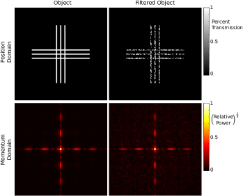
Figure 3: Partial projections of $\bm{\psi}$. The figure simulates the effect of filtering a triple slit object with a $128\times 128$ pixel random, binary pattern. The momentum images are given as relative powers; where their maximum value is scaled to unity. A square-root color mapping emphasizes weaker momentum values. The filtered momentum distribution is a slightly noisy version of the true momentum distribution.

Because the filtered momentum distribution is only lightly perturbed, very little information about the position distribution can be extracted from each CCD image. To maximize the usefulness of this information, we turn to compressive sensing Baraniuk (2007, 2008); Romberg (2008). Compressive sensing Donoho (2006) is an extremely efficient measurement technique for recovering an $N$-dimensional signal from $M<<N$ measurements, provided the signal can be compressed in a known way. The use of outside information, the prior knowledge that a signal is compressible, is a powerful tool for economizing measurement. In the past decade, compressive sensing has taken the signal processing world by storm with applications ranging from magnetic resonance imaging Lustig et al. (2007) to radio astronomy Bobin et al. (2008). More recently, CS has made inroads into the quantum domain with compressive tomography Gross et al. (2010); Cramer et al. (2010); Shabani et al. (2011), and entanglement characterization Howland and Howell (2013). When used for imaging, compressive sensing is closely related to computational imaging Sun et al. (2013); Katz et al. (2009).

Together, the filters and CCD implement a single-pixel camera for the position distribution. The single-pixel camera is the textbook example of compressive sensing and has been extensively investigated Baraniuk (2008); Takhar et al. (2006). Consider the total power $Y_{i}$ striking the CCD while filtering with $f_{i}$, obtained by integrating the $i^{\text{th}}$ momentum image $|\tilde{\psi}_{i}(\vec{k})|^{2}$ over all CCD pixels. The CCD now acts as a single-element power meter. The value $Y_{i}$ is a correlation between the position intensity $|\psi(\vec{x})|^{2}$ and the $i^{\text{th}}$ filter.

These correlations are concisely represented by the series of linear equations

$$\bm{Y}=\bm{FX}.$$ (5)

Here, $\bm{F}$ is an $M\times N$ sensing matrix whose $i^{\text{th}}$ row is a 1D reshaping of the $i^{\text{th}}$ filter function. $\bm{X}$ is an $N$-dimensional vector representing a 1D reshaping of the unknown position distribution $|\psi(\vec{x})|^{2}$, discretized to the same resolution as the filters.

The correlations can be used to iteratively recover $\bm{X}$ by taking a weighted sum of the filter functions

$$\bm{X}=\frac{1}{M}\sum_{i=1}^{M}\bm{Y}_{i}\bm{F}_{i},$$ (6)

but many measurements are required ($M\geq N$) Welsh et al. (2013). Instead, given some reasonable assumptions, compressive sensing dramatically reduces the requisite number of measurements ($M<<N$).

When $M<<N$, Eq. 5 is under-determined; there are many possible $\bm{X}$ consistent with $\bm{Y}$. CS posits that the correct $\bm{X}$ is the one that is sparsest (has the fewest number of non-zero elements) in a representation where $\bm{X}$ is compressible. This $\bm{X}$ is found by solving the regularized least-squares optimization problem

$$\min_{\bm{X}}\frac{\mu}{2}||\bm{Y}-\bm{FX}||_{2}^{2}+TV(\bm{X}),$$ (7)

where for example $||\bm{q}||_{2}^{2}$ is the $\ell_{2}$ norm (Euclidean norm) of $\bm{q}$ and $\mu$ is a constant. The first penalty is a least-squares term that is small when $\bm{X}$ is consistent with the correlation vector $\bm{Y}$. The second penalty $TV(\bm{X})$ is the signal’s total variation,

$$TV(\bm{X})=\sum_{\text{adj. }i,j}|\bm{X}_{i}-\bm{X}_{j}|,$$ (8)

where indices ${i,j}$ run over all pairs of adjacent pixels in $\bm{X}$ so that $TV(\bm{X})$ is just the $\ell_{1}$ norm of $\bm{X}$’s discrete gradient.

If a signal’s total variation is large, values of adjacent pixels vary wildly, indicating a noisy, unstructured signal. Conversely, when a signal’s total variation is small, values for adjacent pixels are strongly correlated, indicating structure consistent with a real image. Put more plainly, we seek the signal with the fewest edges consistent with our measurements; this leverages compressibility in $\bm{X}$’s gradient. Total variation minimization has proven extremely effective for compressive imaging; exact recovery of $\bm{X}$ is possible with $M$ as low as a few percent of $N$ Candes and Tao (2006). In addition to sub-Nyquist sampling, CS has been shown to give a higher signal-to-noise ratio than raster- or basis-scan Candès and Wakin (2008).

We tested our technique on four objects: a double slit, a triple slit, the character $\hbar$, and the University of Rochester logo (Fig. 4). The object and filter masks were introduced using computer controlled spatial light modulators, which can change patterns at typical video speeds up to $60$ Hz. The filter spatial resolution was $N=256\times 256$ pixels. The random filter functions were rows of a randomly permuted, zero-shifted Hadamard matrix Li (2011). This allows $\bm{Y}=\bm{FX}$ to be efficiently computed by a fast transform when solving Eq. 18.

The CCD was a cooled, $12$ bit, $1376\times 1040$ pixel sensor. The exposure time for each CCD image was $10$ ms. The average optical power incident on the CCD was of order $10$ pW. For $10$ ms exposures, each CCD pixel had dark noise $50\pm 10$ in arbitrary power units of $0$ to $4096$. When integrating the CCD image to produce the correlation vector $\bm{Y}$, this value was subtracted. Momentum images are those recorded directly by the camera; no post-processing is performed beyond averaging over all images.

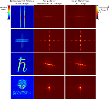
Figure 4: Recovered position and momentum images for four objects. A double slit, triple slit, and $\hbar$ were reconstructed at $N=256\times 256$ resolution from only $M=6553$ filters; the university logo used $M=32768$ filters. No additional post-processing has been performed; position images are those returned by the reconstruction algorithm and momentum images are the recorded single or mean CCD images.

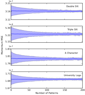
Figure 5: Simulated Momentum MSE: The simulated momentum mean squared errors (MSE) of the four objects used in the experiment are given as a function of the number of random patterns $M$. The shaded region encloses one standard deviation above and below the average MSE for 100 trials. The MSE rapidly approaches a small constant value as the second term of Eq. 4 vanishes. Even for a single pattern, the MSE is at least of order $10^{-7}$.

For the double slit, triple slit, and character objects, $M=0.1N=6553$ filters were used; for the university logo, $M=0.5N=32768$ filters were used. These correspond to total exposure times of $65.5$ sec and $327.7$ sec respectively. Note that Nyquist sampling would require $N$ measurements; for most objects we undersample by an order of magnitude. The requisite $M$ depends both on object complexity and the chosen objective function (Eq. 18), sensing matrix, and solving algorithm. We have chosen conservatively large $M$ to produce high quality images. The dependence of image quality on $M$ is extensively researched; for example see Refs. Candès and Wakin (2008); Romberg (2008); Baraniuk (2008).

The position distributions were reconstructed by solving Eq. 18 using the TVAL3 solver Li et al. (2009). Values of $\mu$ ranged from $2^{10}$ to $2^{14}$. Such large $\mu$ strongly favors the least squares penalty of Eq. 18 such that it is effectively a constraint.

In all cases, our technique recovered high fidelity position and momentum distributions. Even momentum images for a single filter are good approximations to the true distribution; these are further improved by averaging.

To show the accuracy of our technique, Fig. 5 gives the mean squared errors (MSE) of the momentum images for $100$ simulations of the objects used in the experiment as a function of increasing $M$. Even for a single pattern, the MSE is at least of order $10^{-7}$. Averaging over an increasing number of patterns, the middle term of Eq. 4 vanishes and the MSE approaches a constant. This occurs within a few hundred patterns, well before the requisite $M$ for recovering the position image.

We have demonstrated an efficient technique for measuring the probability distributions of complementary observables from a single set of measurements. Beyond fundamental interest, we anticipate that our approach will be useful for a wide variety of quantum and classical sensing tasks, including continuous quantum measurement Jacobs and Steck (2006), high-dimensional entanglement characterization Howland and Howell (2013), wavefront sensing, and phase retrieval Fienup (1982). We strongly emphasize that our technique does not violate the uncertainty principle; at no point does a single detection event give precise information about both position and momentum. Instead, each detection event gives some information about both domains. Our approach economizes the use of this information. More broadly, our system exemplifies a trend in sensing away from traditional strong projective measurements and raster scans which scale poorly to large dimensions. Novel techniques based on compressive sensing, weak measurement, and other unorthodox strategies are necessary to overcome these limitations.

This work was supported by AFOSR grant FA9550-13-1-0019 and DARPA DSO InPho grant W911NF-10-1-0404.

I Supplemental Material

II Theory of Random, Binary Partial Projections

Here we model partial projective measurements in position as random, binary, pixellated filter functions $f_{i}(\vec{x})$, where $i$ is an index for each filter function. We examine the statistics of such random filter functions in transverse-position and transverse-momentum space, and discuss their effect on the momentum probability distribution of an object field, $|\psi(\vec{k})|^{2}$.

II.1 Fourier Transforms of Random Binary Patterns

We model the random filter functions in position space as a sum of Dirac delta functions arranged on a regular lattice, multiplied either by unity with probability $P$ or zero with probability $1-P$;

$$f_{i}(\vec{x})=\sum_{\ell,m}a_{\ell,m}^{(i)}\delta(x-g\ell,y-gm).$$ (9)

Here we have a square lattice of $N$ points centered at $\vec{x}=(0,0)$ with spacing $g$ in the $x$ and $y$ directions. The weights $a_{\ell}^{(i)}$ take values zero or unity according to $P$. Taking the Fourier transform of $f_{i}(\vec{x})$, we find

$$f_{i}(\vec{k})=\frac{1}{2\pi}\sum_{\ell,m}a_{\ell,m}^{(i)}e^{-ig(k_{x}\ell+k_{y}m)}.$$ (10)

To model these filter functions in momentum, we make the following assumptions. First, since $N$ is large, and each weight has probability $P$ of being unity and is otherwise zero, we represent $f_{i}(\vec{k})$ as a sum of $NP$ unit phasors. Therefore, $f_{i}(\vec{k}=0)$ is $NP/2\pi$.

Second, since the weights are randomly distributed, we represent $f_{i}(\vec{k}\neq 0)$ as a sum of $NP$ random phasors. This sum is well described by a two-dimensional, complex random walk with unit step size McCrea and Whipple (1940); Tse (2005). Therefore, nonzero frequency components have zero-mean and average square-magnitude $NP/(2\pi)^{2}$. When $NP$ is large, it follows from the central limit theorem that the non-zero frequency components are described by a circularly symmetric, complex Gaussian distribution with real and imaginary widths $\sigma$. The momentum amplitude distribution of a typical filter is a sharply peaked function centered at the origin.

$f_{i}(\vec{k})$ can now be written as a weighted sum of a Dirac delta function $\delta(\vec{k})$ and a noise function $\phi_{i}(\vec{k})$ whose phases vary uniformly;

$$f_{i}(\vec{k})\approx\alpha\delta(\vec{k})+\beta\phi_{i}(\vec{k}),$$ (11)

where $\alpha$ and $\beta$ are parameters we estimate from the pattern-averaged values of $f_{i}(\vec{k})$ and $|f_{i}(\vec{k})|^{2}$. Values for $\phi_{i}(\vec{k})$ follow a random, complex Gaussian white noise distribution, with real and imaginary parts of zero mean and $\sigma=1/\sqrt{2}$.

Knowing $f_{i}(\vec{k}=0)=NP/2\pi$ gives $\alpha=NP/2\pi$. Knowing that $\langle f_{i}(\vec{k}\neq 0)\rangle=0$, and that $\langle|f_{i}(\vec{k}\neq 0)|^{2}\rangle=NP/(2\pi)^{2}$, we have that $\beta=\sqrt{NP}/2\pi$, where $\langle\cdot\rangle$ is an average over many filter functions. Therefore, a viable model for $f_{i}(\vec{k})$ is

$$f_{i}(\vec{k})\approx\frac{NP}{2\pi}\delta(\vec{k})+\frac{\sqrt{NP}}{2\pi}\phi_{i}(\vec{k}).$$ (12)

As mentioned previously, our model assumes that $f_{i}(\vec{k})$ is a sum of $NP$ random phasors. However, since we are sampling these phasors without replacement, $\langle|f_{i}(\vec{k}\neq 0)|^{2}\rangle$ is actually less than $NP/(2\pi)^{2}$; $NP/(2\pi)^{2}$ is a conservative estimate which will over-estimate the perturbation to $|\psi(\vec{k})|^{2}$ due to $f_{i}(\vec{k})$.

II.2 Effect of a random pattern on momentum distribution

Let $\psi(\vec{x})$ be the unperturbed position amplitude of the field. After interacting with filter $f_{i}(\vec{x})$, the perturbed position amplitude is $\tilde{\psi}(\vec{x})=f_{i}(\vec{x})\psi(\vec{x})$. Therefore, the perturbed momentum amplitude is $\tilde{\psi}(\vec{k})=\psi(\vec{k})\ast f_{i}(\vec{k})$, where $\ast$ denotes convolution.

Using Eq. (12), we find

$$\tilde{\psi}(\vec{k})=\frac{NP}{2\pi}(\psi(\vec{k})\ast\delta(\vec{k}))+\frac{\sqrt{NP}}{2\pi}(\psi(\vec{k})\ast\phi_{i}(\vec{k})).$$ (13)

Since the first term is a convolution with a delta function, we find

$$\tilde{\psi}(\vec{k})=\frac{NP}{2\pi}\psi(\vec{k})+\frac{\sqrt{NP}}{2\pi}(\psi(\vec{k})\ast\phi_{i}(\vec{k})).$$ (14)

Taking the modulus square of $\tilde{\psi}(\vec{k})$ gives us the perturbed momentum distribution

$$|\tilde{\psi}(\vec{k})|^{2} =\mathcal{N}\bigg{[}|\psi(\vec{k})|^{2}+\frac{1}{NP}|(\psi(\vec{k})\ast\phi_{i}(\vec{k}))|^{2}+$$

$$+2\frac{1}{\sqrt{NP}}\mathbf{Re}[\psi^{*}(\vec{k})(\psi(\vec{k})\ast\phi_{i}(\vec{k}))]\bigg{]},$$ (15)

where $\mathcal{N}$ is a normalization constant.

To see how $|\tilde{\psi}(\vec{k})|^{2}$ compares to the unperturbed probability distribution $|\psi(\vec{k})|^{2}$, it suffices to know that $|(\psi(\vec{k})\ast\phi_{i}(\vec{k}))|^{2}$ and $[\psi^{*}(\vec{k})(\psi(\vec{k})\ast\phi_{i}(\vec{k}))]$ are both of the order unity. As $NP$ becomes large, $\frac{1}{\sqrt{NP}}$ becomes small, and $|\tilde{\psi}(\vec{k})|^{2}$ approaches $|\psi(\vec{k})|^{2}$.

More importantly, we recover $|\psi(\vec{k})|^{2}$ (up to a uniform constant) from averaging $|\tilde{\psi}(\vec{k})|^{2}$ over a large number $M$ of different filter functions $f_{i}$. Since the mean value of $\phi_{i}(\vec{k})$ is zero, this averaging results in an approximation to $|\psi(\vec{k})|^{2}$ as an incoherent sum of the two terms,

$$\langle|\tilde{\psi}(\vec{k})|^{2}\rangle_{M}\approx\mathcal{N^{\prime}}\bigg{[}|\psi(\vec{k})|^{2}+\frac{1}{NP}\langle|(\psi(\vec{k})\ast\phi_{i}(\vec{k}))|^{2}\rangle_{M}\bigg{]},$$ (16)

where $\langle\cdot\rangle_{M}$ is an average over $M$ filter functions.

III Compressive Sensing

Compressive sensing (CS) is a measurement technique that uses optimization to obtain a $N$-dimensional signal $\bm{X}$ from $M<<N$ linear projections (linear measurements) Baraniuk (2007); Candes and Tao (2006). CS exploits prior-knowledge about the signal’s compressibility to require fewer measurements than the Nyquist limit. The measurement process is

$$\bm{Y}=\bm{FX}+\bm{\Gamma},$$ (17)

where $\bm{Y}$ is an $M$-dimensional vector of measurements, $\bm{F}$ is an $M\times N$ sensing matrix, and $\bm{\Gamma}$ is an $M$-dimensional noise vector. Each measured value $\bm{Y}_{i}$ is therefore the inner-product of $\bm{X}$ with sensing vector $\bm{F}_{i}$, where $i$ is an index over rows of $\bm{F}$.

Because $M<<N$, $\bm{Y}$ does not uniquely specify $\bm{X}$. CS proposes that the correct $\bm{X}$ is the one which is most compressible by a method expected to compress it. Most commonly, one must know a basis or transformation in which $\bm{X}$ is expected to be sparse (have few nonzero coefficients). For images, typical sparse representations include discrete cosines, various wavelets, and the discrete gradient Romberg (2008).

This correct $\bm{X}$ is found by minimizing the objective function

$$\min_{\bm{X}}\frac{\mu}{2}||\bm{Y}-\bm{FX}||_{2}^{2}+g(\bm{X}),$$ (18)

where for example $||\bm{Q}||_{2}^{2}$ is the $\ell_{2}$ (Euclidean) norm of $\bm{Q}$ and $\mu$ is a scalar constant. The first penalty is a least-squares penalty; it ensures the recovered $\bm{X}$ is consistent with the measurements. The second penalty $g(\bm{X})$ is a term which gets smaller the more compressible $\bm{X}$ is. Typical $g(\bm{X})$ include the $\ell_{1}$ norm of $\bm{\Phi X}$

$$g(\bm{X})=||\bm{\Phi}\bm{X}||_{1}=\sum_{i=1}^{M}|\bm{\Phi}\bm{X}|,$$ (19)

where $\bm{\Phi}$ is a transform to a sparse basis (wavelets, cosines), and $\bm{X}$’s total variation

$$g(\bm{X})=TV(\bm{X})=\sum_{\text{adj. }i,j}|\bm{X}_{i}-\bm{X}_{j}|,$$ (20)

where $i$ and $j$ run over pairs of adjacent pixels in $\bm{X}$. This is the $\ell_{1}$ norm of $\bm{X}$’s discrete gradient Wang et al. (2008). The $\ell_{1}$ norm is a useful measure of sparsity because it makes Eq. 18 convex and therefore easy to solve.

To minimize the required number of measurements $M$, the sensing vectors $\bm{F}_{i}$ should be mutually unbiased with the sparse transform; this gives the counter-intuitive result that random sensing vectors are extremely effective in almost all cases. For a $K$-sparse signal ($K$ nonzero entries in the sparse representation), CS can give an exact reconstruction with only $M\propto K\log(N/K)$ measurements Candès et al. (2006). In practice, $M$ can be as small as a few percent of $N$.

III.1 Single-Pixel Camera

The most illustrative example of compressive sensing is the Rice single-pixel camera Baraniuk (2008). The camera is composed of a single pixel detector, a digital micro-mirror device (DMD), and an imaging lens. A DMD is a mirror array composed of thousands of mirrors. Each mirror acts as a reflective pixel with values on and off, reflecting into and away from the single-pixel detector respectively. The lens images an object onto the DMD array while the DMD displays a random pattern corresponding to a row in the sensing matrix $\bm{F}$. The single-pixel detector records the intensity of light as a projection of the random pattern with the object for all $M$ patterns resulting in a $\bm{Y}$ vector of length $M$. The sensing matrix $\bm{F}$ and the measurement vector $\bm{Y}$ are fed into an algorithm to minimize equation (18).

References

- Bohr (1928) N. Bohr, Nature (London) 121, 580 (1928).
- Platt et al. (2001) B. C. Platt et al., Journal of Refractive Surgery 17, S573 (2001).
- Maassen and Uffink (1988) H. Maassen and J. B. Uffink, Physical Review Letters 60, 1103 (1988).
- Hall (1995) M. J. Hall, Physical review letters 74, 3307 (1995).
- Lundeen et al. (2011) J. S. Lundeen, B. Sutherland, A. Patel, C. Stewart, and C. Bamber, Nature 474, 188 (2011).
- Kocsis et al. (2011) S. Kocsis, B. Braverman, S. Ravets, M. J. Stevens, R. P. Mirin, L. K. Shalm, and A. M. Steinberg, Science 332, 1170 (2011).
- Dressel et al. (2013) J. Dressel, M. Malik, F. M. Miatto, A. N. Jordan, and R. W. Boyd, arXiv preprint arXiv:1305.7154 (2013).
- Donoho (2006) D. L. Donoho, Information Theory, IEEE Transactions on 52, 1289 (2006).
- Goodman (2005) J. W. Goodman, Introduction to Fourier optics (Roberts and Company Publishers, 2005).
- McCrea and Whipple (1940) W. McCrea and F. Whipple, in Proc. Roy. Soc. Edinburgh, Vol. 60 (1940) pp. 281–298.
- Tse (2005) D. Tse, Fundamentals of wireless communication (Cambridge university press, 2005).
- Baraniuk (2007) R. Baraniuk, IEEE signal processing magazine 24 (2007).
- Baraniuk (2008) R. G. Baraniuk, IEEE Signal Processing Magazine (2008).
- Romberg (2008) J. Romberg, IEEE Signal Processing Magazine 25, 14 (2008).
- Lustig et al. (2007) M. Lustig, D. Donoho, and J. M. Pauly, Magnetic resonance in medicine 58, 1182 (2007).
- Bobin et al. (2008) J. Bobin, J.-L. Starck, and R. Ottensamer, Selected Topics in Signal Processing, IEEE Journal of 2, 718 (2008).
- Gross et al. (2010) D. Gross, Y.-K. Liu, S. T. Flammia, S. Becker, and J. Eisert, Phys. Rev. Lett. 105, 150401 (2010).
- Cramer et al. (2010) M. Cramer, M. B. Plenio, S. T. Flammia, R. Somma, D. Gross, S. D. Bartlett, O. Landon-Cardinal, D. Poulin, and Y.-K. Liu, Nature communications 1, 149 (2010).
- Shabani et al. (2011) A. Shabani, R. Kosut, M. Mohseni, H. Rabitz, M. Broome, M. Almeida, A. Fedrizzi, and A. White, Physical review letters 106, 100401 (2011).
- Howland and Howell (2013) G. A. Howland and J. C. Howell, Physical Review X 3, 011013 (2013).
- Sun et al. (2013) B. Sun, M. P. Edgar, R. Bowman, L. E. Vittert, S. Welsh, A. Bowman, and M. Padgett, Science 340, 844 (2013).
- Katz et al. (2009) O. Katz, Y. Bromberg, and Y. Silberberg, Applied Physics Letters 95, 131110 (2009).
- Takhar et al. (2006) D. Takhar, J. N. Laska, M. B. Wakin, M. F. Duarte, D. Baron, S. Sarvotham, K. F. Kelly, and R. G. Baraniuk, in Electronic Imaging 2006 (International Society for Optics and Photonics, 2006) pp. 606509–606509.
- Welsh et al. (2013) S. S. Welsh, M. P. Edgar, R. Bowman, P. Jonathan, B. Sun, and M. J. Padgett, Optics express 21, 23068 (2013).
- Candes and Tao (2006) E. J. Candes and T. Tao, Information Theory, IEEE Transactions on 52, 5406 (2006).
- Candès and Wakin (2008) E. J. Candès and M. B. Wakin, Signal Processing Magazine, IEEE 25, 21 (2008).
- Li (2011) C. Li, Compressive sensing for 3D data processing tasks: applications, models and algorithms, Ph.D. thesis, Rice University (2011).
- Li et al. (2009) C. Li, W. Yin, and Y. Zhang, CAAM Report (2009).
- Jacobs and Steck (2006) K. Jacobs and D. A. Steck, Contemporary Physics 47, 279 (2006).
- Fienup (1982) J. R. Fienup, Applied optics 21, 2758 (1982).
- Wang et al. (2008) Y. Wang, J. Yang, W. Yin, and Y. Zhang, SIAM Journal on Imaging Sciences 1, 248 (2008).
- Candès et al. (2006) E. J. Candès, J. Romberg, and T. Tao, Information Theory, IEEE Transactions on 52, 489 (2006).