SISSA 26/2016/FISI

IPMU16-0064

Predictions for the Majorana CP Violation Phases in the

Neutrino Mixing Matrix and Neutrinoless Double Beta Decay
I. Girardi$\mbox{}^{a)}$, S. T. Petcov$\mbox{}^{a,b)}$  and A. V. Titov$\mbox{}^{a)}$

^a SISSA/INFN, Via Bonomea 265, 34136 Trieste, Italy

^b Kavli IPMU (WPI), University of Tokyo, 5-1-5 Kashiwanoha, 277-8583 Kashiwa, Japan

We obtain predictions for the Majorana phases $\alpha_{21}/2$ and $\alpha_{31}/2$ of the $3\times 3$ unitary neutrino mixing matrix $U=U_{e}^{\dagger}\,U_{\nu}$, $U_{e}$ and $U_{\nu}$ being the $3\times 3$ unitary matrices resulting from the diagonalisation of the charged lepton and neutrino Majorana mass matrices, respectively. We focus on forms of $U_{e}$ and $U_{\nu}$ permitting to express $\alpha_{21}/2$ and $\alpha_{31}/2$ in terms of the Dirac phase $\delta$ and the three neutrino mixing angles of the standard parametrisation of $U$, and the angles and the two Majorana-like phases $\xi_{21}/2$ and $\xi_{31}/2$ present, in general, in $U_{\nu}$. The concrete forms of $U_{\nu}$ considered are fixed by, or associated with, symmetries (tri-bimaximal, bimaximal, etc.), so that the angles in $U_{\nu}$ are fixed. For each of these forms and forms of $U_{e}$ that allow to reproduce the measured values of the three neutrino mixing angles $\theta_{12}$, $\theta_{23}$ and $\theta_{13}$, we derive predictions for phase differences $(\alpha_{21}/2-\xi_{21}/2)$, $(\alpha_{31}/2-\xi_{31}/2)$, etc., which are completely determined by the values of the mixing angles. We show that the requirement of generalised CP invariance of the neutrino Majorana mass term implies $\xi_{21}=0$ or $\pi$ and $\xi_{31}=0$ or $\pi$. For these values of $\xi_{21}$ and $\xi_{31}$ and the best fit values of $\theta_{12}$, $\theta_{23}$ and $\theta_{13}$, we present predictions for the effective Majorana mass in neutrinoless double beta decay for both neutrino mass spectra with normal and inverted ordering.

Keywords: neutrino physics, leptonic CP violation, Majorana phases, sum rules, neutrinoless double beta decay, discrete flavour symmetries, generalised CP symmetry.

1 Introduction

Determining the status of the CP symmetry in the lepton sector, discerning the type of spectrum the neutrino masses obey, identifying the nature — Dirac or Majorana — of massive neutrinos and determining the absolute neutrino mass scale are among the highest priority goals of the programme of future research in neutrino physics (see, e.g., [1]). The results obtained within this ambitious research programme can shed light, in particular, on the origin of the observed pattern of neutrino mixing. Comprehending the origin of the patterns of neutrino masses and mixing is one of the most challenging problems in neutrino physics. It is an integral part of the more general fundamental problem in particle physics of deciphering the origins of flavour, i.e., of the patterns of quark, charged lepton and neutrino masses and of the quark and neutrino mixing.

In refs. [2, 3, 4, 5] (see also [6]), working in the framework of the reference 3-neutrino mixing scheme (see, e.g., [1]), we have derived predictions for the Dirac CP violation (CPV) phase in the Pontecorvo, Maki, Nakagawa and Sakata (PMNS) neutrino mixing matrix within the discrete flavour symmetry approach to neutrino mixing. This approach provides a natural explanation of the observed pattern of neutrino mixing and is widely explored at present (see, e.g., [7, 8] and references therein). In the present article, using the method developed and utilised in [2], we derive predictions for the Majorana CPV phases in the PMNS matrix [9] within the same approach based on discrete flavour symmetries. Our study is a natural continuation of the studies performed in [2, 3, 4, 5, 6].

As is well known, the PMNS matrix will contain physical CPV Majorana phases if the massive neutrinos are Majorana particles [9]. The massive neutrinos are predicted to be Majorana fermions by a large number of theories of neutrino mass generation (see, e.g., [7, 10, 11]), most notably, by the theories based on the seesaw mechanism [12]. The flavour neutrino oscillation probabilities do not depend on the Majorana phases [9, 13]. The Majorana phases play particularly important role in processes involving real or virtual neutrinos, which are characteristic of Majorana nature of massive neutrinos and in which the total lepton charge $L$ changes by two units, $|\Delta L|=2$ (see, e.g., [14]). One widely discussed and experimentally relevant example is neutrinoless double beta ($(\beta\beta)_{0\nu}$-) decay of even-even nuclei (see, e.g., [10, 15, 16]) ${}^{48}Ca$, ${}^{76}Ge$, ${}^{82}Se$, ${}^{100}Mo$, ${}^{130}Te$, ${}^{136}Xe$, etc.: $(A,Z)\rightarrow(A,Z+2)+e^{-}+e^{-}$. The predictions for the rates of the lepton flavour violating processes, $\mu\rightarrow e+\gamma$ and $\mu\rightarrow 3e$ decays, $\mu-e$ conversion in nuclei, etc., in theories of neutrino mass generation with massive Majorana neutrinos (e.g., TeV scale type I seesaw model, the Higgs triplet model, etc.) depend on the Majorana phases (see, e.g., [17, 18]). And the Majorana phases in the PMNS matrix can provide the CP violation necessary for the generation of the observed baryon asymmetry of the Universe [19] .

In the reference case of 3-neutrino mixing, which we are going to consider in the present article, there can be two physical Majorana CPV phases in the PMNS neutrino mixing matrix in addition to the Dirac CPV phase [9]. The PMNS matrix in this case is given by

$$U=VQ\,,\quad Q=\operatorname{diag}\left(1,e^{i\frac{\alpha_{21}}{2}},e^{i\frac{\alpha_{31}}{2}}\right)\,,$$ (1)

where $\alpha_{21,31}$ are the two Majorana CPV phases and $V$ is a CKM-like matrix containing the Dirac CPV phase. The matrix $V$ has the following form in the standard parametrisation of the PMNS matrix [1], which we are going to employ in what follows:

$$\begin{array}[]{c}V=\left(\begin{array}[]{ccc}c_{12}c_{13}&s_{12}c_{13}&s_{13}e^{-i\delta}\\[5.69046pt] -s_{12}c_{23}-c_{12}s_{23}s_{13}e^{i\delta}&c_{12}c_{23}-s_{12}s_{23}s_{13}e^{i\delta}&s_{23}c_{13}\\[5.69046pt] s_{12}s_{23}-c_{12}c_{23}s_{13}e^{i\delta}&-c_{12}s_{23}-s_{12}c_{23}s_{13}e^{i\delta}&c_{23}c_{13}\\ \end{array}\right)\,.\end{array}$$ (2)

Here $0\leq\delta\leq 2\pi$ is the Dirac CPV phase and we have used the standard notation $c_{ij}=\cos\theta_{ij}$, $s_{ij}=\sin\theta_{ij}$ with $0\leq\theta_{ij}\leq\pi/2$. In the case of CP invariance we have $\delta=0$, $\pi$, $2\pi$, $0$ and $2\pi$ being physically indistinguishable, and [22] $\alpha_{21}=k\pi$, $\alpha_{31}=k^{\prime}\pi$, $k,k^{\prime}=0,1,2$ .

The neutrino mixing parameters $\sin^{2}\theta_{12}$, $\sin^{2}\theta_{23}$ and $\sin^{2}\theta_{13}$ play important role in our further considerations. They were determined with relatively small uncertainties in the most recent analysis of the global neutrino oscillation data performed in [24] (for earlier analyses see, e.g., [25, 26]). The authors of ref. [24], using, in particular, the first NO$\nu$A (LID) data on $\nu_{\mu}\rightarrow\nu_{e}$ oscillations from [27], find the following best fit values and 3$\sigma$ allowed ranges of $\sin^{2}\theta_{12}$, $\sin^{2}\theta_{23}$ and $\sin^{2}\theta_{13}$:

$$(\sin^{2}\theta_{12})_{\rm BF}=0.297\,,~{}~{}~{}~{}0.250\leq\sin^{2}\theta_{12}\leq 0.354\,,$$ (3)

$$(\sin^{2}\theta_{23})_{\rm BF}=0.437~{}(0.569)\,,~{}~{}~{}~{}0.379~{}(0.383)\leq\sin^{2}\theta_{23}\leq 0.616~{}(0.637)\,,$$ (4)

$$(\sin^{2}\theta_{13})_{\rm BF}=0.0214~{}(0.0218)\,,~{}~{}~{}~{}0.0185~{}(0.0186)\leq\sin^{2}\theta_{13}\leq 0.0246~{}(0.0248)\,.$$ (5)

The values (values in brackets) correspond to neutrino mass spectrum with normal ordering (inverted ordering) (see, e.g., [1]), denoted further as the NO (IO) spectrum. Note, in particular, that $\sin^{2}\theta_{23}$ can differ significantly from 0.5 and that $\sin^{2}\theta_{23}=0.5$ lies in the $2\sigma$ interval of allowed values. Using the same set of data the authors of [24] find also the following best fit value and $2\sigma$ allowed range of the Dirac phase $\delta$:

$$\delta=1.35\,\pi~{}(1.32\,\pi)\,,~{}~{}~{}~{}0.92\,\pi~{}(0.83\,\pi)\leq\delta\leq 1.99\,\pi\,.$$ (6)

The discrete flavour symmetry approach to neutrino mixing is based on the observation that the PMNS neutrino mixing angles $\theta_{12}$, $\theta_{23}$ and $\theta_{13}$ have values which differ from those of specific symmetry forms of the mixing matrix by subleading perturbative corrections (see further). The fact that the PMNS matrix in the case of 3-neutrino mixing is a product of two $3\times 3$ unitary matrices $U_{e}$ and $U_{\nu}$, originating from the diagonalisation of the charged lepton and neutrino mass matrices,

$$U=U_{e}^{\dagger}\,U_{\nu}\,,$$ (7)

is also widely exploited. In terms of the parameters of $U_{e}$ and $U_{\nu}$, in the absence of constraints the PMNS matrix can be parametrised as [28]

$$U=U_{e}^{\dagger}\,U_{\nu}=(\tilde{U}_{e})^{\dagger}\,\Psi\,\tilde{U}_{\nu}\,Q_{0}\,.$$ (8)

Here $\tilde{U}_{e}$ and $\tilde{U}_{\nu}$ are CKM-like $3\times 3$ unitary matrices, and $\Psi$ and $Q_{0}$ are given by

$$\Psi={\rm diag}\left(1,\text{e}^{-i\psi},\text{e}^{-i\omega}\right)\,,\quad Q_{0}={\rm diag}\left(1,\text{e}^{i\frac{\xi_{21}}{2}},\text{e}^{i\frac{\xi_{31}}{2}}\right)\,,$$ (9)

where $\psi$, $\omega$, $\xi_{21}$ and $\xi_{31}$ are phases which contribute to physical CPV phases. The phases in $Q_{0}$ result from the diagonalisation of the neutrino Majorana mass term and contribute to the Majorana phases in the PMNS matrix.

In the approach of interest one assumes the existence at certain energy scale of a (lepton) flavour symmetry corresponding to a non-Abelian discrete group $G_{f}$. The symmetry group $G_{f}$ can be broken, in general, to different symmetry subgroups, or “residual symmetries”, $G_{e}$ and $G_{\nu}$ of the charged lepton and neutrino mass terms, respectively. Given a discrete symmetry $G_{f}$, there are more than one (but still a finite number of) possible residual symmetries $G_{e}$ and $G_{\nu}$. The subgroup $G_{e}$, in particular, can be trivial. Non-trivial residual symmetries $G_{e}$ and $G_{\nu}$ (of a given $G_{f}$) constrain the forms of the matrices $U_{e}$ and $U_{\nu}$, and thus the form of $U$.

Among the widely considered symmetry forms of $U$ are: i) the tri-bimaximal (TBM) form [30, 29], ii) the bimaximal (BM) form  [32], iii) the golden ratio type A (GRA) form [33, 34], iv) the golden ratio type B (GRB) form [35], and v) the hexagonal (HG) form [36, 37]. It is typically assumed that the matrix $\tilde{U}_{\nu}$ in eq. (8), and not $\tilde{U}_{e}$, has a symmetry form and, in particular, has one of the forms discussed above. For all these forms we have

$$\tilde{U}_{\nu}=R_{23}(\theta^{\nu}_{23})\,R_{12}(\theta^{\nu}_{12})\,,$$ (10)

with $\theta^{\nu}_{23}=-\,\pi/4$, $R_{23}$ and $R_{12}$ being $3\times 3$ orthogonal matrices describing rotations in the 2-3 and 1-2 planes:

$$R_{12}\left(\theta^{\nu}_{12}\right)=\begin{pmatrix}\cos\theta^{\nu}_{12}&\sin\theta^{\nu}_{12}&0\\ -\sin\theta^{\nu}_{12}&\cos\theta^{\nu}_{12}&0\\ 0&0&1\end{pmatrix}\,,\quad R_{23}\left(\theta^{\nu}_{23}\right)=\begin{pmatrix}1&0&0\\ 0&\cos\theta^{\nu}_{23}&\sin\theta^{\nu}_{23}\\ 0&-\sin\theta^{\nu}_{23}&\cos\theta^{\nu}_{23}\\ \end{pmatrix}\,.$$ (11)

The value of the angle $\theta^{\nu}_{12}$, and thus of $\sin^{2}\theta^{\nu}_{12}$, depends on the form of $\tilde{U}_{\nu}$. For the TBM, BM, GRA, GRB and HG forms we have: i) $\sin^{2}\theta^{\nu}_{12}=1/3$ (TBM), ii) $\sin^{2}\theta^{\nu}_{12}=1/2$ (BM), iii) $\sin^{2}\theta^{\nu}_{12}=(2+r)^{-1}\cong 0.276$ (GRA), $r$ being the golden ratio, $r=(1+\sqrt{5})/2$, iv) $\sin^{2}\theta^{\nu}_{12}=(3-r)/4\cong 0.345$ (GRB), and v) $\sin^{2}\theta^{\nu}_{12}=1/4$ (HG).

The TBM form of $\tilde{U}_{\nu}$, for example, can be obtained from a $G_{f}=A_{4}$ symmetry, when the residual symmetry is $G_{\nu}=Z_{2}$. In this case there is an additional accidental $\mu-\tau$ symmetry, which together with the $Z_{2}$ symmetry leads to the TBM form of $\tilde{U}_{\nu}$ (see, e.g., [38]). The TBM form can also be derived from $G_{f}=T^{\prime}$ with $G_{\nu}=Z_{2}$, provided the left-handed (LH) charged lepton and neutrino fields each transform as triplets of $T^{\prime}$ . One can obtain the BM form from, e.g., the $G_{f}=S_{4}$ symmetry, when $G_{\nu}=Z_{2}$. There is an accidental $\mu-\tau$ symmetry in this case as well [40]. The $A_{5}$ symmetry group can be utilised to generate GRA mixing, while the groups $D_{10}$ and $D_{12}$ can lead to the GRB and HG mixing forms, respectively.

The symmetry forms of $\tilde{U}_{\nu}$ considered above do not include rotation in the 1-3 plane, i.e., $\theta^{\nu}_{13}=0$. However, forms of $\tilde{U}_{\nu}$ of the type

$$\tilde{U}_{\nu}=R_{23}(\theta^{\nu}_{23})\,R_{13}(\theta^{\nu}_{13})\,R_{12}(\theta^{\nu}_{12})\,,$$ (12)

with non-zero values of $\theta^{\nu}_{13}$ are inspired by certain types of flavour symmetries (see, e.g., [41, 42, 43, 44]). In [41], for example, the so-called tri-permuting pattern, corresponding to $\theta^{\nu}_{12}=\theta^{\nu}_{23}=-\pi/4$ and $\theta^{\nu}_{13}=\sin^{-1}(1/3)$, was proposed and investigated. In the study we will perform we will consider also the form in eq. (12) for three representative values of $\theta^{\nu}_{13}$ discussed in the literature: $\theta^{\nu}_{13}=\pi/20$, $\pi/10$ and $\sin^{-1}(1/3)$.

The symmetry values of the angles in the matrix $\tilde{U}_{\nu}$ typically, and in all cases considered above, differ by relatively small perturbative corrections from the experimentally determined values of at least some of the angles $\theta_{12}$, $\theta_{23}$ and $\theta_{13}$. The requisite corrections are provided by the matrix $U_{e}$, or equivalently, by $\tilde{U}_{e}$. In the approach followed in [2, 3, 6, 4] we are going to adopt, the matrix $\tilde{U}_{e}$ is unconstrained and was chosen on phenomenological grounds. This corresponds to the case of trivial subgroup $G_{e}$, i.e., of the charged lepton mass term breaking the symmetry $G_{f}$ completely. The matrix $\tilde{U}_{e}$ in the general case depends on three angles and one phase [28]. However, in a class of theories of (lepton) flavour and neutrino mass generation, based on a GUT and/or a discrete symmetry (see, e.g., [45, 46, 47, 48, 49, 50]), $\tilde{U}_{e}$ is an orthogonal matrix which describes one rotation in the 1-2 plane,

$$\tilde{U}_{e} =R^{-1}_{12}(\theta^{e}_{12})\,,$$ (13)

or two rotations in the planes 1-2 and 2-3,

$$\tilde{U}_{e} =R^{-1}_{23}(\theta^{e}_{23})\,R^{-1}_{12}(\theta^{e}_{12})\,,$$ (14)

$\theta^{e}_{12}$ and $\theta^{e}_{23}$ being the corresponding rotation angles. Other possibilities include $\tilde{U}_{e}$ being an orthogonal matrix which describes i) one rotation in the 1-3 plane ,

$$\tilde{U}_{e} =R^{-1}_{13}(\theta^{e}_{13})\,,$$ (15)

or ii) two rotations in any other two of the three planes, e.g.,

$$\tilde{U}_{e} =R^{-1}_{23}(\theta^{e}_{23})\,R^{-1}_{13}(\theta^{e}_{13})\,,~{}~{}{\rm or}$$ (16)

$$\tilde{U}_{e} =R^{-1}_{13}(\theta^{e}_{13})\,R^{-1}_{12}(\theta^{e}_{12})\,.$$ (17)

We use the inverse matrices in eqs. (13) – (17) for convenience of the notations in expressions that will appear further in our analysis.

In refs. [2, 4] sum rules for the cosine of the Dirac phase $\delta$ of the PMNS matrix, by which $\cos\delta$ is expressed in terms of the three measured neutrino angles $\theta_{12}$, $\theta_{23}$ and $\theta_{13}$, were derived in the cases of the following forms of $\tilde{U}_{e}$ and $\tilde{U}_{\nu}$:

• $\tilde{U}_{\nu}=R_{23}(\theta^{\nu}_{23})R_{12}(\theta^{\nu}_{12})$  and  i) $\tilde{U}_{e}=R^{-1}_{12}(\theta^{e}_{12})$,  ii) $\tilde{U}_{e}=R^{-1}_{13}(\theta^{e}_{13})$,  iii) $\tilde{U}_{e}=R^{-1}_{23}(\theta^{e}_{23})R^{-1}_{12}(\theta^{e}_{12})$,  iv) $\tilde{U}_{e}=R^{-1}_{23}(\theta^{e}_{23})R^{-1}_{13}(\theta^{e}_{13})$,  v) $\tilde{U}_{e}=R^{-1}_{13}(\theta^{e}_{13})R^{-1}_{12}(\theta^{e}_{12})$;

• $\tilde{U}_{\nu}=R_{23}(\theta^{\nu}_{23})R_{13}(\theta^{\nu}_{13})R_{12}(\theta^{\nu}_{12})$  and  vi) $\tilde{U}_{e}=R^{-1}_{12}(\theta^{e}_{12})$,  vii) $\tilde{U}_{e}=R^{-1}_{13}(\theta^{e}_{13})$.

The sum rules thus found allowed us in the cases of the TBM, BM (LC), GRA, GRB and HG mixing forms of $\tilde{U}_{\nu}$ in item A and for certain fixed values of $\theta^{\nu}_{ij}$ in item B to obtain predictions for $\cos\delta$ (see refs. [2, 3, 4, 6]) as well as for the rephasing invariant

$$J_{\rm CP}={\rm Im}\left\{U^{*}_{e1}U^{*}_{\mu 3}U_{e3}U_{\mu 1}\right\}=\frac{1}{8}\sin\delta\sin 2\theta_{13}\sin 2\theta_{23}\sin 2\theta_{12}\cos\theta_{13}\,,$$ (18)

on which the magnitude of CP-violating effects in neutrino oscillations depends [51]. The results of these studies showed that the predictions for $\cos\delta$ exhibit strong dependence on the symmetry form of $\tilde{U}_{\nu}$. This led to the conclusion that a sufficiently precise measurement of $\cos\delta$ combined with high precision measurements of $\sin^{2}\theta_{12}$, $\sin^{2}\theta_{23}$ and $\sin^{2}\theta_{13}$ can allow to test critically the idea of existence of an underlying discrete symmetry form of the PMNS matrix and, thus, of existence of a new symmetry in particle physics.

In ref. [2] predictions for the Majorana phases of the PMNS matrix $\alpha_{21}$ and $\alpha_{31}$ in the case of $\tilde{U}_{\nu}=R_{23}(\theta^{\nu}_{23})R_{12}(\theta^{\nu}_{12})$, corresponding to the TBM, BM (LC), GRA, GRB and HG symmetry forms, and $\tilde{U}_{e}=R^{-1}_{23}(\theta^{e}_{23})R^{-1}_{12}(\theta^{e}_{12})$ were derived under the assumption that the phases $\xi_{21}$ and $\xi_{31}$ in eqs. (8) and (9), which originate from the diagonalisation of the neutrino Majorana mass term, are known (i.e., are fixed by symmetry or other arguments). In the present article we extend the analysis performed in [2] to obtain predictions for the phases $\alpha_{21}$ and $\alpha_{31}$ in the cases of the forms of the matrices $\tilde{U}_{\nu}$ and $\tilde{U}_{e}$ listed in items A and B above. This allows us to obtain predictions for the phase differences $(\alpha_{21}-\xi_{21})$ and $(\alpha_{31}-\xi_{31})$. We further employ the generalised CP symmetry constraint in the neutrino sector [52, 53, 54], which allows us to fix the values of the phases $\xi_{21}$ and $\xi_{31}$, and thus to predict the values of $\alpha_{21}$ and $\alpha_{31}$. We use these results together with the sum rule results on $\cos\delta$ to derive (in graphic form) predictions for the dependence of the absolute value of the $(\beta\beta)_{0\nu}$-decay effective Majorana mass (see, e.g., [10]), $\left|\langle\!\,m\,\!\rangle\right|$, on the lightest neutrino mass in all cases considered for both the NO and IO spectra.

Our article is organised as follows. In Section 2 we obtain sum rules for $(\alpha_{21}-\xi_{21})$ and $(\alpha_{31}-\xi_{31})$ in schemes containing one rotation from the charged lepton sector, i.e., $\tilde{U}_{e}=R^{-1}_{12}(\theta^{e}_{12})$, or $\tilde{U}_{e}=R^{-1}_{13}(\theta^{e}_{13})$, and two rotations from the neutrino sector: $\tilde{U}_{\nu}=R_{23}(\theta^{\nu}_{23})\,R_{12}(\theta^{\nu}_{12})$. In these schemes the PMNS matrix has the form

$$U=R_{ij}(\theta^{e}_{ij})\,\Psi\,R_{23}(\theta^{\nu}_{23})\,R_{12}(\theta^{\nu}_{12})\,Q_{0}\,,$$ (19)

with $(ij)=(12)$, $(13)$. We obtain results in the general case of arbitrary fixed values of $\theta^{\nu}_{23}$ and $\theta^{\nu}_{12}$. In Section 3 we analyse schemes with $\tilde{U}_{e}=R^{-1}_{23}(\theta^{e}_{23})\,R^{-1}_{12}(\theta^{e}_{12})$, $\tilde{U}_{e}=R^{-1}_{23}(\theta^{e}_{23})\,R^{-1}_{13}(\theta^{e}_{13})$, or $\tilde{U}_{e}=R^{-1}_{13}(\theta^{e}_{13})\,R^{-1}_{12}(\theta^{e}_{12})$, and  two rotations from the neutrino sector, i.e.,

$$U=R_{ij}(\theta^{e}_{ij})\,R_{kl}(\theta^{e}_{kl})\,\Psi\,R_{23}(\theta^{\nu}_{23})\,R_{12}(\theta^{\nu}_{12})\,Q_{0}\,,$$ (20)

with $(ij)-(kl)=(12)-(23)$, $(13)-(23)$, $(12)-(13)$. Again we provide results for arbitrary fixed values of $\theta^{\nu}_{23}$ and $\theta^{\nu}_{12}$. Further, in Section 4, we extend the analysis performed in Section 2 to the case of a third rotation matrix present in $\tilde{U}_{\nu}$:

$$U=R_{ij}(\theta^{e}_{ij})\,\Psi\,R_{23}(\theta^{\nu}_{23})\,R_{13}(\theta^{\nu}_{13})\,R_{12}(\theta^{\nu}_{12})\,Q_{0}\,,$$ (21)

with $(ij)=(12)$, $(13)$, $(23)$. Section 5 contains a brief summary of the sum rules for the Majorana phases $\alpha_{21}/2$ and $\alpha_{31}/2$ derived in Sections 2 – 4. Using the sum rules, we present in Section 6 predictions for phase differences $(\alpha_{21}/2-\xi_{21}/2)$, $(\alpha_{31}/2-\xi_{31}/2)$, etc., involving the Majorana phases $\alpha_{21}/2$ and $\alpha_{31}/2$, which are determined just by the values of the three neutrino mixing angles $\theta_{12}$, $\theta_{23}$ and $\theta_{13}$, and of the fixed angles $\theta^{\nu}_{ij}$. In the cases listed in item A we give results for values of $\theta^{\nu}_{23}$ ($=-\,\pi/4$) and $\theta^{\nu}_{12}$, corresponding to the TBM, BM (LC), GRA, GRB and HG symmetry forms of $\tilde{U}_{\nu}$. In each of the two cases given in item B the reported results are for $\theta^{\nu}_{23}=-\,\pi/4$ and five sets of values of $\theta^{\nu}_{13}$ and $\theta^{\nu}_{12}$ associated with symmetries. We then set $(\xi_{21},\xi_{31})=(0,0)$, $(0,\pi)$, $(\pi,0)$ and $(\pi,\pi)$ and use the resulting values of $\alpha_{21}/2$ and $\alpha_{31}/2$ to derive graphical predictions for the absolute value of the effective Majorana mass in $(\beta\beta)_{0\nu}$-decay, $\left|\langle\!\,m\,\!\rangle\right|$, as a function of the lightest neutrino mass in the schemes of mixing studied. We show in Section 7 that the requirement of generalised CP invariance of the neutrino Majorana mass term in the cases of $S_{4}$, $A_{4}$, $T^{\prime}$ and $A_{5}$ lepton flavour symmetries leads indeed to $\xi_{21}=0$ or $\pi$, $\xi_{31}=0$ or $\pi$. In the first two cases (third case) studied in Section 3, B1 and B2 (B3), the phase $\alpha_{31}/2$ (the phases $\delta$, $\alpha_{21}/2$ and $\alpha_{31}/2$) depends (depend) on an additional phase, $\beta$ ($\omega$), which, in general, is not constrained. For schemes B1 and B2, the predictions for $\left|\langle\!\,m\,\!\rangle\right|$ are obtained in Section 6 by varying $\beta$ in the interval $[0,\pi]$. In the case of scheme B3 the results for the Majorana phases and $\left|\langle\!\,m\,\!\rangle\right|$ are derived for the value of $\omega=0$, for which the Dirac phase $\delta$ has a value in its $2\sigma$ allowed interval quoted in eq. (6). Section 8 contains summary of the results of the present study and conclusions.

We note finally that the titles of Sections 2 – 4 and of their subsections reflect the rotations contained in the corresponding parametrisation, eqs. (19) – (21).

2 The Cases of $\boldsymbol{\theta^{e}_{ij}-(\theta^{\nu}_{23},\theta^{\nu}_{12})}$ Rotations

In this section we derive the sum rules for $\alpha_{21}$ and $\alpha_{31}$ of interest in the case when the matrix $\tilde{U}_{\nu}=R_{23}(\theta^{\nu}_{23})\,R_{12}(\theta^{\nu}_{12})$ with fixed (e.g., symmetry) values of the angles $\theta^{\nu}_{23}$ and $\theta^{\nu}_{12}$, gets correction only due to one rotation from the charged lepton sector. The neutrino mixing matrix $U$ has the form given in eq. (19). We do not consider the case of eq. (19) with $(ij)=(23)$, because in this case the reactor angle $\theta_{13}=0$ and thus the measured value of $\theta_{13}\cong 0.15$ cannot be reproduced.

2.1 The Scheme with $\boldsymbol{\theta^{e}_{12}-(\theta^{\nu}_{23},\theta^{\nu}_{12})}$ Rotations (Case A1)

In the present subsection we consider the parametrisation of the neutrino mixing matrix given in eq. (19) with $(ij)=(12)$. In this parametrisation the PMNS matrix has the form

$$U=R_{12}(\theta^{e}_{12})\,\Psi\,R_{23}(\theta^{\nu}_{23})\,R_{12}(\theta^{\nu}_{12})\,Q_{0}\,.$$ (22)

The phase $\omega$ in the phase matrix $\Psi$ is unphysical.

We are interested in deriving analytic expressions for the Majorana phases $\alpha_{21}$ and $\alpha_{31}$ i) in terms of the parameters of the parametrisation in eq. (22), $\theta^{e}_{12}$, $\psi$, $\theta^{\nu}_{23}$, $\theta^{\nu}_{12}$, $\xi_{21}$ and $\xi_{31}$, and possibly ii) in terms of the angles $\theta_{12}$, $\theta_{13}$, $\theta_{23}$ and the Dirac phase $\delta$ of the standard parametrisation of the PMNS matrix, the fixed angles $\theta^{\nu}_{23}$ and $\theta^{\nu}_{12}$, and the phases $\xi_{21}$ and $\xi_{31}$. The values of the phases $\alpha_{21}$ and $\alpha_{31}$ in the latter case, as we will see, indeed depend on the value of the Dirac phase $\delta$. Thus, we first recall the sum rule satisfied by the Dirac phase $\delta$ in the case under study, by which $\cos\delta$ is expressed in terms of the angles $\theta_{12}$, $\theta_{13}$ and $\theta_{23}$. The sum rule of interest reads [2]:

$$\cos\delta=\frac{\tan\theta_{23}}{\sin 2\theta_{12}\sin\theta_{13}}\,\left[\cos 2\theta^{\nu}_{12}+\left(\sin^{2}\theta_{12}-\cos^{2}\theta^{\nu}_{12}\right)\,\left(1-\cot^{2}\theta_{23}\,\sin^{2}\theta_{13}\right)\right]\,.$$ (23)

Although the expression in eq. (23) was derived in [2] for $\theta^{\nu}_{23}=-\pi/4$, it was shown in [4] to be valid for arbitrary $\theta^{\nu}_{23}$. The dependence of $\cos\delta$ on $\theta^{\nu}_{23}$ is “hidden”, in particular, in the specific relation between $\theta_{23}$ and $\theta^{\nu}_{23}$:

$$\sin^{2}\theta_{23} =\frac{|U_{\mu 3}|^{2}}{1-|U_{e3}|^{2}}=\frac{\sin^{2}\theta^{\nu}_{23}-\sin^{2}\theta_{13}}{1-\sin^{2}\theta_{13}}\,.$$ (24)

We give also the expressions of $\sin^{2}\theta_{13}$ and $\sin^{2}\theta_{12}$ in terms of the parameters of the parametrisation of the PMNS matrix given in eq. (22), which will be used further in the analysis performed in this subsection:

$$\sin^{2}\theta_{13} =|U_{e3}|^{2}=\sin^{2}\theta^{e}_{12}\sin^{2}\theta^{\nu}_{23}\,,$$ (25)

$$\sin^{2}\theta_{12} =\frac{|U_{e2}|^{2}}{1-|U_{e3}|^{2}}=\frac{1}{1-\sin^{2}\theta_{13}}\bigg{[}\cos^{2}\theta^{\nu}_{23}\sin^{2}\theta^{e}_{12}\cos^{2}\theta^{\nu}_{12}+\cos^{2}\theta^{e}_{12}\sin^{2}\theta^{\nu}_{12}$$

$$+\dfrac{1}{2}\sin 2\theta^{e}_{12}\sin 2\theta^{\nu}_{12}\cos\theta^{\nu}_{23}\cos\psi\bigg{]}\,.$$ (26)

The parameters $\sin^{2}\theta^{\nu}_{23}$ and $\sin^{2}\theta^{e}_{12}$ can be expressed in terms of $\sin^{2}\theta_{13}$ and $\sin^{2}\theta_{23}$ using eqs. (24) and  (25).

From eqs. (25) and (26) we get the following expression for $\cos\psi$:

$$\cos\psi=\dfrac{\sin^{2}\theta^{\nu}_{23}\left(\cos^{2}\theta_{13}\sin^{2}\theta_{12}-\sin^{2}\theta^{\nu}_{12}\right)+\sin^{2}\theta_{13}\left(\cos^{2}\theta^{\nu}_{12}\sin^{2}\theta^{\nu}_{23}-\cos 2\theta^{\nu}_{12}\right)}{{\rm sgn}(\sin 2\theta^{e}_{12})\,\sin 2\theta^{\nu}_{12}\cos\theta^{\nu}_{23}\sin\theta_{13}\left(\sin^{2}\theta^{\nu}_{23}-\sin^{2}\theta_{13}\right)^{1/2}}\,.$$ (27)

The sign of $\sin 2\theta^{e}_{12}$ is supposed to be fixed in the underlying theory leading to the neutrino mixing given in eq. (22). In what follows we will account for both possibilities of $\sin 2\theta^{e}_{12}>0$ and $\sin 2\theta^{e}_{12}<0$. Using eq. (24) and setting $\sin^{2}\theta^{\nu}_{23}=\sin^{2}\theta_{23}\cos^{2}\theta_{13}+\sin^{2}\theta_{13}$, $\cos\theta^{\nu}_{23}=\cos\theta_{23}\cos\theta_{13}$ and ${\rm sgn}(\sin 2\theta^{e}_{12})=1$ in eq. (27) leads to an expression for $\cos\psi$ in terms of $\theta^{\nu}_{12}$ and the standard parametrisation mixing angles $\theta_{12}$, $\theta_{13}$ and $\theta_{23}$, which coincides with the expression for $\cos\phi$ given in eq. (22) in [2]. For $\theta^{\nu}_{23}=-\pi/4$, eq. (27) reduces to the expression for $\cos\phi$ in eq. (46) in ref. [2] and in eq. (37) in ref. [3].

The cosine of the phase $\psi$ can be determined uniquely using eq. (27), i.e., using as input ${\rm sgn}(\sin 2\theta^{e}_{12})$, the symmetry values of $\theta^{\nu}_{12}$ and $\theta^{\nu}_{23}$ (of $\theta^{\nu}_{12}$) and the measured value of $\theta_{12}$ and $\theta_{13}$ ($\theta_{12}$, $\theta_{13}$ and $\theta_{23}$). However, the sign of $\sin\psi$ in this case remains unfixed if no additional information allowing to fix it is available. This in turn leads to an ambiguity in the determination of the phase $\psi$ from the value of $\cos\psi$: in the interval $[0,2\pi]$, two values of $\psi$ will be possible.

Sum rules for the Majorana phases $\alpha_{21}$ and $\alpha_{31}$ of the type we are interested in were derived in [2]. The sum rules for $\alpha_{21}$ and $\alpha_{31}$ we are aiming to obtain in this subsection turn out to be a particular case of the sum rules derived in [2]. This becomes clear from a comparison of eq. (18) in [2], which fixes the parametrisation of $U$ used in [2], and the expression for $U$ in eq. (22). It shows that to get the sum rules for $\alpha_{21}$ and $\alpha_{31}$ of interest, one has formally to set $\hat{\theta}_{23}=\theta^{\nu}_{23}$, $\phi=-\psi$ and $\beta=0$ in the sum rules for $\alpha_{21}$ and $\alpha_{31}$ derived in eq. (102) in [2] and to take into account the two possible signs of the product $c^{e}_{12}c^{\nu}_{23}s^{\nu}_{23}\equiv\cos\theta^{e}_{12}\cos\theta^{\nu}_{23}\sin\theta^{\nu}_{23}$:

$$\frac{\alpha_{21}}{2}=\beta_{e2}-\beta_{e1}+\frac{\xi_{21}}{2}\,,~{}~{}~{}$$ (28)

$$\frac{\alpha_{31}}{2}=\beta_{e2}+\tilde{\varphi}+\frac{\xi_{31}}{2}\,,\quad e^{i\tilde{\varphi}}={\rm sgn}(c^{e}_{12}c^{\nu}_{23}s^{\nu}_{23})=+1~{}{\rm or}~{}(-1)\,.$$ (29)

Thus, $\tilde{\varphi}=0$ or $\pi$. The results in eqs. (28) and (29) can be obtained formally from eqs. (88), (89) and (95) in [2] by setting $\hat{\theta}_{23}=\theta^{\nu}_{23}$, $\phi=-\psi$, $Q_{1}={\rm diag}(1,1,1)$ and $Q_{2}={\rm diag}(1,e^{i(\beta_{e2}-\beta_{e1})},{\rm sgn}(c^{e}_{12}c^{\nu}_{23}s^{\nu}_{23})\,e^{i\beta_{e2}})$. We note that in the case considered of arbitrary fixed signs of $c^{e}_{12}$, $s^{e}_{12}\equiv\sin\theta^{e}_{12}$, $c^{\nu}_{23}$ and $s^{\nu}_{23}$, the $U_{e3}$ element of the PMNS matrix in eq. (95) in [2] must also be replaced by $U_{e3}\,{\rm sgn}(c^{e}_{12}s^{e}_{12}c^{\nu}_{23})$. Correspondingly, in terms of the parametrisation in eq. (22) of the PMNS matrix, the phases $\beta_{e2}$ and $\beta_{e1}$ are given by eqs. (90) and (91) in [2]:

$$\beta_{e1} ={\rm arg}(U_{e1})={\rm arg}\left(c^{e}_{12}c^{\nu}_{12}-s^{e}_{12}c^{\nu}_{23}s^{\nu}_{12}e^{-i\psi}\right)\,,$$ (30)

$$\beta_{e2} ={\rm arg}(U_{e2}\,e^{-i\frac{\xi_{21}}{2}})={\rm arg}\left(c^{e}_{12}s^{\nu}_{12}+s^{e}_{12}c^{\nu}_{23}c^{\nu}_{12}e^{-i\psi}\right)\,,$$ (31)

where $c^{\nu}_{12}\equiv\cos\theta^{\nu}_{12}$ and $s^{\nu}_{12}\equiv\sin\theta^{\nu}_{12}$. For $\tilde{\varphi}=0$, eq. (29) reduces to the expression for $\alpha_{31}/2$ in eq. (102) in [2]. By using eq. (25), $s^{e}_{12}$ and $c^{e}_{12}$ in eqs. (30) and (31) can be expressed (given their signs) in terms of $\sin\theta_{13}$ and $\sin\theta^{\nu}_{23}$, while the phase $\psi$ is determined via eq. (27) by the values of $\theta_{12}$, $\theta_{13}$, $\theta^{\nu}_{12}$ and $\theta^{\nu}_{23}$ (up to an ambiguity of the sign of $\sin\psi$). The phases $\beta_{e2}$ and $\beta_{e1}$ in this case will be given in terms of $\theta_{12}$, $\theta_{13}$, $\theta^{\nu}_{12}$ and $\theta^{\nu}_{23}$, i.e., in terms of mixing angles which are measured or fixed by symmetry arguments. It is often convenient to express $\sin\theta^{\nu}_{23}$ and $\cos\theta^{\nu}_{23}$ in terms of the measured angles $\theta_{13}$ and $\theta_{23}$ of the standard parametrisation of the PMNS matrix using the relation in eq. (24).

As can be shown employing the formalism developed in [2] and taking into account the possibility of negative signs of $c^{e}_{12}s^{\nu}_{12}$ and $c^{e}_{12}c^{\nu}_{12}$, the expressions for the phases $\beta_{e2}$ and $\beta_{e1}$ in terms of the angles $\theta_{12}$, $\theta_{13}$, $\theta_{23}$ and the Dirac phase $\delta$ of the standard parametrisation of the PMNS matrix have the form:

$$\beta_{e2} ={\rm arg}\left(U_{\tau 1}{\rm sgn}(c^{e}_{12}s^{\nu}_{12})\right)={\rm arg}\left[\left(s_{12}s_{23}-c_{12}c_{23}s_{13}e^{i\delta}\right){\rm sgn}(c^{e}_{12}s^{\nu}_{12})\right]\,,$$ (32)

$$\beta_{e1} ={\rm arg}\left(U_{\tau 2}\,e^{i\pi}{\rm sgn}(c^{e}_{12}c^{\nu}_{12})\,e^{-i\frac{\alpha_{21}}{2}}\right)={\rm arg}\left[\left(c_{12}s_{23}+s_{12}c_{23}s_{13}e^{i\delta}\right){\rm sgn}(c^{e}_{12}c^{\nu}_{12})\right]\,.$$ (33)

For ${\rm sgn}(c^{e}_{12}s^{\nu}_{12})=1$ and ${\rm sgn}(c^{e}_{12}c^{\nu}_{12})=1$, eqs. (32) and (33) reduce respectively to eqs. (100) and (101) in ref. [2].

It follows from eqs. (32) and (33) that the phases $\beta_{e1}$ and $\beta_{e2}$ are determined by the values of the standard parametrisation mixing angles $\theta_{12}$, $\theta_{13}$, $\theta_{23}$ and of the Dirac phase $\delta$. The phase $\delta$ is also determined (up to a sign ambiguity of $\sin\delta$) by the values of “standard” angles $\theta_{12}$, $\theta_{13}$, $\theta_{23}$ via the sum rule given in eq. (23). Since the relations in eqs. (28) and (29) between the Majorana phases $\alpha_{21}$ and $\alpha_{31}$ and the phases $\beta_{e1}$ and $\beta_{e2}$ involve the phases $\xi_{21}$ and $\xi_{31}$ originating from the diagonalisation of the neutrino Majorana mass term, $\alpha_{21}$ and $\alpha_{31}$ will be determined by the values of the “standard” neutrino mixing angles $\theta_{12}$, $\theta_{13}$, $\theta_{23}$ (up to the mentioned ambiguity related to the undetermined so far sign of $\sin\delta$), provided the values of $\xi_{21}$ and $\xi_{31}$ are known. Thus, predictions for the Majorana phases $\alpha_{21}$ and $\alpha_{31}$ can be obtained when the phases $\xi_{21}$ and $\xi_{31}$ are fixed by additional considerations of, e.g., generalised CP invariance, symmetries, etc. In theories with discrete lepton flavour symmetries the phases $\xi_{21}$ and $\xi_{31}$ are often determined by the employed symmetries of the theory (see, e.g., [49, 50, 45, 55, 56] and references quoted therein). We will show in Section 7 how the phases $\xi_{21}$ and $\xi_{31}$ are fixed by the requirement of generalised CP invariance of the neutrino Majorana mass term in the cases of the non-Abelian discrete flavour symmetries $S_{4}$, $A_{4}$, $T^{\prime}$ and $A_{5}$. In all these cases the generalised CP invariance constraint fixes the values of $\xi_{21}$ and $\xi_{31}$, which allows us to obtain predictions for the Majorana phases $\alpha_{21}$ and $\alpha_{31}$.

The phases $\beta_{e1}$, $\beta_{e2}$, $\psi$ and $\delta$ can be shown to satisfy the relation:

$$\delta=\psi+\beta_{e1}+\beta_{e2}+\varphi\,,\quad e^{i\varphi}={\rm sgn}(c^{e}_{12}s^{e}_{12}c^{\nu}_{23})=+1~{}{\rm or}~{}(-1)\,.$$ (34)

For $\varphi=0$ (${\rm sgn}(c^{e}_{12}s^{e}_{12}c^{\nu}_{23})=+1$), this relation reduces to eq. (94) in ref. [2] by setting $\psi=-\phi$. From eqs. (28), (29) and (34) we get further

$$(\alpha_{31}-\xi_{31})-\frac{1}{2}\,(\alpha_{21}-\xi_{21})=\beta_{e1}+\beta_{e2}+2\tilde{\varphi}=\delta-\psi-\varphi\,,\quad\varphi=0~{}{\rm or}~{}\pi\,,$$ (35)

where we took into account that $2\tilde{\varphi}=0$ or $2\pi$.

The Dirac phase $\delta$ and the phase $\psi$ are related [2]. We will give below only the relation between $\sin\delta$ and $\sin\psi$. It can be obtained from eq. (28) in [2] by setting  $\phi=-\psi$ and by taking into account that in the case considered both signs of $\sin 2\theta^{e}_{12}\cos\theta^{\nu}_{23}$ are, in principle, allowed :

$$\sin\delta= \;{\rm sgn}\,(\sin 2\theta^{e}_{12}\cos\theta^{\nu}_{23})\,\frac{\sin 2\theta^{\nu}_{12}}{\sin 2\theta_{12}}\,\sin\psi\,.$$ (36)

We note that within the approach employed in our analysis, the results presented in eqs. (28) – (36) are exact and are valid for arbitrary fixed values of $\theta^{\nu}_{12}$ and $\theta^{\nu}_{23}$ and for arbitrary signs of $\sin\theta^{e}_{12}$ and $\cos\theta^{e}_{12}$ ($|\sin\theta^{e}_{12}|$ and $|\cos\theta^{e}_{12}|$ can be expressed in terms of $\theta_{13}$ and $\theta^{\nu}_{23}$).

Although the sum rules derived above allow to determine the values of the Majorana phases $\alpha_{21}$ and $\alpha_{31}$ (up to a two-fold ambiguity related to the ambiguity of ${\rm sgn}(\sin\delta)$ or of ${\rm sgn}(\sin\psi)$) if the phases $\xi_{21}$ and $\xi_{31}$ are known, we will present below an alternative method of determination of $\alpha_{21}$ and $\alpha_{31}$, which can be used in the cases when the method developed in [2] cannot be applied. The alternative method makes use of the rephasing invariants associated with the two Majorana phases of the PMNS matrix.

In the case of 3-neutrino mixing under discussion there are, in principle, three independent CPV rephasing invariants. The first is associated with the Dirac phase $\delta$ and is given by the well-known expression in eq. (18), where we have shown also the expression of the $J_{\rm CP}$ factor in the standard parametrisation. The other two, $I_{1}$ and $I_{2}$, are related to the two Majorana CPV phases in the PMNS matrix and can be chosen as [57, 58, 15] :

$$I_{1}={\rm Im}\left\{U_{e1}^{\ast}\,U_{e2}\right\}\,,\quad I_{2}={\rm Im}\left\{U_{e1}^{\ast}\,U_{e3}\right\}\,.$$

The rephasing invariants associated with the Majorana phases are not uniquely determined. Instead of $I_{1}$ defined above we could have chosen, e.g., $I^{\prime}_{1}={\rm Im}\left\{U_{\tau 1}^{\ast}\,U_{\tau 2}\right\}$ or $I^{\prime\prime}_{1}={\rm Im}\left\{U_{\mu 1}U_{\mu 2}^{\ast}\right\}$, while instead of $I_{2}$ we could have used $I^{\prime}_{2}={\rm Im}\left\{U_{\tau 2}^{\ast}\,U_{\tau 3}\right\}$, or $I^{\prime\prime}_{2}={\rm Im}\left\{U_{\mu 2}\,U_{\mu 3}^{\ast}\right\}$. However, the three invariants — $J_{\rm CP}$ and any two chosen Majorana phase invariants — form a complete set in the case of 3-neutrino mixing: any other two rephasing invariants associated with the Majorana phases can be expressed in terms of the two chosen Majorana phase invariants and the $J_{\rm CP}$ factor [57]. We note also that CP violation due to the Majorana phase $\alpha_{21}$ requires that both $I_{1}={\rm Im}\left\{U^{\ast}_{e1}U_{e2}\right\}\neq 0$ and ${\rm Re}\left\{U^{\ast}_{e1}U_{e2}\right\}\neq 0$ [58]. Similarly, $I_{2}={\rm Im}\left\{U_{e1}^{\ast}U_{e3}\right\}\neq 0$ would imply violation of the CP symmetry only if in addition ${\rm Re}\left\{U_{e1}^{\ast}U_{e3}\right\}\neq 0$.

In the standard parametrisation of the PMNS matrix $U$, the rephasing invariants $I_{1}$ and $I_{2}$ are given by

$$I_{1} =\cos\theta_{12}\sin\theta_{12}\cos^{2}\theta_{13}\sin(\alpha_{21}/2)\,,$$ (37)

$$I_{2} =\cos\theta_{12}\sin\theta_{13}\cos\theta_{13}\sin(\alpha_{31}/2-\delta)\,.$$ (38)

Comparing these expressions with the expressions for $I_{1}$ and $I_{2}$ in the parametrisation of $U$ defined in eq. (22), we obtain sum rules for $\sin(\alpha_{21}/2)$ and $\sin(\alpha_{31}/2-\delta)$ in terms of $\theta^{e}_{12}$, $\psi$, $\theta^{\nu}_{12}$, $\theta^{\nu}_{23}$ and the standard parametrisation mixing angles $\theta_{12}$ and $\theta_{13}$:

$$\sin(\alpha_{21}/2) =\dfrac{1}{\cos^{2}\theta_{13}\sin 2\theta_{12}}\bigg{[}\sin 2\theta^{e}_{12}\cos\theta^{\nu}_{23}\big{(}\sin(\xi_{21}/2-\psi)-2\sin^{2}\theta^{\nu}_{12}\cos\psi\sin(\xi_{21}/2)\big{)}$$

$$+\sin 2\theta^{\nu}_{12}\sin(\xi_{21}/2)\big{(}\cos^{2}\theta^{e}_{12}-\sin^{2}\theta^{e}_{12}\cos^{2}\theta^{\nu}_{23}\big{)}\bigg{]}\,,$$ (39)

$$\sin(\alpha_{31}/2-\delta) =\dfrac{2\sin\theta^{e}_{12}\sin\theta^{\nu}_{23}}{\cos\theta_{12}\sin 2\theta_{13}}\bigg{[}\cos\theta^{e}_{12}\cos\theta^{\nu}_{12}\sin(\xi_{31}/2-\psi)-\cos\theta^{\nu}_{23}\sin\theta^{e}_{12}\sin\theta^{\nu}_{12}\sin(\xi_{31}/2)\bigg{]}\,.$$ (40)

The result in eq. (40) can be derived also from eqs. (29) and (34), which lead to

$$\frac{\alpha_{31}}{2}-\delta=-\,\psi-\,\beta_{e1}+\,\tilde{\varphi}-\,\varphi+\frac{\xi_{31}}{2}\,,$$ (41)

and by using further eq. (30) for $\beta_{e1}$. The expression for $\sin(\alpha_{31}/2)$, which can be obtained from eqs. (29) and (31), has a form similar to that of $\sin(\alpha_{31}/2-\delta)$:

$$\sin(\alpha_{31}/2) =\dfrac{{\rm sgn}(c^{e}_{12}c^{\nu}_{23}s^{\nu}_{23})}{\sin\theta_{12}\cos\theta_{13}}\bigg{[}\sin\theta^{e}_{12}\cos\theta^{\nu}_{12}\cos\theta^{\nu}_{23}\sin(\xi_{31}/2-\psi)+\cos\theta^{e}_{12}\sin\theta^{\nu}_{12}\sin(\xi_{31}/2)\bigg{]}\,.$$ (42)

The angles $\theta^{\nu}_{12}$ and $\theta^{\nu}_{23}$ in eqs. (2.1), (40) and (42), as we have already emphasised, are assumed to be fixed by symmetry arguments, $\theta^{e}_{12}$ can be expressed in terms of $\theta_{13}$ and $\theta^{\nu}_{23}$ using eq. (25), while eq. (27) allows to express $\psi$ in terms of $\theta_{12}$, $\theta_{13}$, $\theta^{\nu}_{12}$ and $\theta^{\nu}_{23}$. The formulae for $\cos(\alpha_{21}/2)$ and $\cos(\alpha_{31}/2-\delta)$, which enter into the expression for the absolute value of the effective Majorana mass in $(\beta\beta)_{0\nu}$-decay (see, e.g., [15]), $\left|\langle\!\,m\,\!\rangle\right|$, can be obtained from eqs. (2.1) and (40) by changing $\xi_{21}$ to $\xi_{21}+\pi$ and $\xi_{31}$ to $\xi_{31}+\pi$, respectively.

In terms of the standard parametrisation mixing angles $\theta_{12}$, $\theta_{13}$, $\theta_{23}$ and the Dirac phase $\delta$, and the angles $\theta^{\nu}_{12}$ and $\theta^{\nu}_{23}$, the expressions for $\sin(\alpha_{21}/2)$ and $\sin(\alpha_{31}/2)$ read:

$$\sin(\alpha_{21}/2) =\dfrac{1}{\sin^{2}\theta^{\nu}_{23}\sin 2\theta^{\nu}_{12}}\bigg{[}\sin 2\theta_{23}\sin\theta_{13}\big{(}\sin(\xi_{21}/2-\delta)-2\cos^{2}\theta_{12}\cos\delta\sin(\xi_{21}/2)\big{)}$$

$$+\sin(\xi_{21}/2)\sin 2\theta_{12}\big{(}\sin^{2}\theta_{23}-\cos^{2}\theta_{23}\sin^{2}\theta_{13}\big{)}\bigg{]}\,,$$ (43)

$$\sin(\alpha_{31}/2) =\dfrac{{\rm sgn}(c^{\nu}_{23})}{\sin\theta^{\nu}_{12}\sin\theta^{\nu}_{23}}\bigg{[}\sin\theta_{12}\sin\theta_{23}\sin(\xi_{31}/2)-\cos\theta_{12}\cos\theta_{23}\sin\theta_{13}\sin(\xi_{31}/2+\delta)\bigg{]}\,,$$ (44)

where, we recall, $\sin^{2}\theta^{\nu}_{23}=1-\cos^{2}\theta_{23}\cos^{2}\theta_{13}$.

The phases $\xi_{21}$ and $\xi_{31}$, as we have already discussed, are supposed to be fixed by symmetry arguments. Thus, it proves convenient to have analytic expressions which allow to calculate the phase differences $(\alpha_{21}/2-\xi_{21}/2)$, $(\alpha_{31}/2-\delta-\xi_{31}/2)$ and $(\alpha_{31}/2-\xi_{31}/2)$. We find for $\sin(\alpha_{21}/2-\xi_{21}/2)$, $\sin(\alpha_{31}/2-\delta-\xi_{31}/2)$ and $\sin(\alpha_{31}/2-\xi_{31}/2)$:

$$\sin(\alpha_{21}/2-\xi_{21}/2) =-\,\dfrac{\sin 2\theta^{e}_{12}}{\cos^{2}\theta_{13}\sin 2\theta_{12}}\cos\theta^{\nu}_{23}\sin\psi=-\,\dfrac{\sin 2\theta_{23}\sin\theta_{13}}{\sin^{2}\theta^{\nu}_{23}\sin 2\theta^{\nu}_{12}}\,\sin\delta\,,$$ (45)

$$\sin(\alpha_{31}/2-\delta-\xi_{31}/2) =-\,\dfrac{\sin 2\theta^{e}_{12}}{\cos\theta_{12}\sin 2\theta_{13}}\,\cos\theta^{\nu}_{12}\sin\theta^{\nu}_{23}\,\sin\psi\,$$

$$=-\,{\rm sgn}(\cos\theta^{\nu}_{23})\,\dfrac{\sin\theta_{12}\sin\theta_{23}}{\sin\theta^{\nu}_{12}\sin\theta^{\nu}_{23}}\,\sin\delta\,,$$ (46)

$$\sin(\alpha_{31}/2-\xi_{31}/2) =-\,\dfrac{{\rm sgn}(c^{e}_{12}c^{\nu}_{23}s^{\nu}_{23})}{\sin\theta_{12}\cos\theta_{13}}\,\sin\theta^{e}_{12}\cos\theta^{\nu}_{12}\cos\theta^{\nu}_{23}\sin\psi$$

$$=-\dfrac{{\rm sgn}(\cos\theta^{\nu}_{23})}{\sin\theta^{\nu}_{12}\sin\theta^{\nu}_{23}}\,\sin\theta_{13}\cos\theta_{12}\cos\theta_{23}\sin\delta\,.$$ (47)

It follows from eqs. (45) and (47) that $|\sin(\alpha_{21(31)}/2-\xi_{21(31)}/2)|\propto\sin\theta_{13}$. Using the results given, e.g., in eqs. (28), (29), (32), (33), (23), and the best fit values of the neutrino oscillation parameters quoted in eqs. (3) – (5), we can obtain predictions for the values of the phases $(\alpha_{21}/2-\xi_{21}/2)$ and $(\alpha_{31}/2-\xi_{31}/2)$ for the symmetry forms of $\tilde{U}_{\nu}$ (TBM, BM (LC), GRA, etc.) considered. These predictions as well as predictions for the values of $(\alpha_{21}/2-\xi_{21}/2)$ and $(\alpha_{31}/2-\xi_{31}/2)$ in the cases investigated in the next subsection and in Sections 3 and 4 will be presented in Section 6.

2.2 The Scheme with $\boldsymbol{\theta^{e}_{13}-(\theta^{\nu}_{23},\theta^{\nu}_{12})}$ Rotations (Case A2)

In the present subsection we consider the parametrisation of the neutrino mixing matrix given in eq. (19) with $(ij)=(13)$. In this parametrisation the PMNS matrix has the form

$$U=R_{13}(\theta^{e}_{13})\,\Psi\,R_{23}(\theta^{\nu}_{23})\,R_{12}(\theta^{\nu}_{12})\,Q_{0}\,.$$ (48)

Now the phase $\psi$ in the phase matrix $\Psi$ is unphysical. We employ the approaches used in the preceding subsection, which are based on the method developed in [2] and on the relevant rephasing invariants, for determining the Majorana phases $\alpha_{21}$ and $\alpha_{31}$.

We first give the expressions for $\sin^{2}\theta_{13}$, $\sin^{2}\theta_{23}$ and $\sin^{2}\theta_{12}$ in terms of the parameters of the parametrisation in eq. (48), which will be used in our analysis:

$$\sin^{2}\theta_{13} =|U_{e3}|^{2}=\sin^{2}\theta^{e}_{13}\cos^{2}\theta^{\nu}_{23}\,,$$ (49)

$$\sin^{2}\theta_{23} =\frac{|U_{\mu 3}|^{2}}{1-|U_{e3}|^{2}}=\frac{\sin^{2}\theta^{\nu}_{23}}{1-\sin^{2}\theta_{13}}\,,$$ (50)

$$\sin^{2}\theta_{12} =\frac{|U_{e2}|^{2}}{1-|U_{e3}|^{2}}=\frac{1}{1-\sin^{2}\theta_{13}}\bigg{[}\sin^{2}\theta^{\nu}_{23}\sin^{2}\theta^{e}_{13}\cos^{2}\theta^{\nu}_{12}$$

$$+\cos^{2}\theta^{e}_{13}\sin^{2}\theta^{\nu}_{12}-\dfrac{1}{2}\sin 2\theta^{e}_{13}\sin 2\theta^{\nu}_{12}\sin\theta^{\nu}_{23}\cos\omega\bigg{]}\,.$$ (51)

The formulae for $\sin^{2}\theta_{13}$ and $\sin^{2}\theta_{23}$ given above have been derived in [4]. The expression for $\sin^{2}\theta_{12}$ is a generalisation to arbitrary fixed values of $\theta^{\nu}_{23}$ of that derived in [4] for $\theta^{\nu}_{23}=-\pi/4$.

From eqs. (49) and (51) we obtain an expression for $\cos\omega$ in terms of the measured mixing angles $\theta_{12}$ and $\theta_{13}$, and the known $\theta^{\nu}_{12}$ and $\theta^{\nu}_{23}$:

$$\cos\omega =-\dfrac{\cos^{2}\theta^{\nu}_{23}\left(\cos^{2}\theta_{13}\sin^{2}\theta_{12}-\sin^{2}\theta^{\nu}_{12}\right)+\sin^{2}\theta_{13}\left(\sin^{2}\theta^{\nu}_{12}-\cos^{2}\theta^{\nu}_{12}\sin^{2}\theta^{\nu}_{23}\right)}{{\rm sgn}(\sin 2\theta^{e}_{13})\sin 2\theta^{\nu}_{12}\sin\theta^{\nu}_{23}\sin\theta_{13}\left(\cos^{2}\theta^{\nu}_{23}-\sin^{2}\theta_{13}\right)^{1/2}}\,.$$ (52)

For $\theta^{\nu}_{23}=-\pi/4$ and ${\rm sgn}(\sin 2\theta^{e}_{13})=1$, this sum rule reduces to the sum rule for $\cos\omega$ given in eq. (25) in [4].

As we will see, the expressions for the Majorana phases $\alpha_{21}$ and $\alpha_{31}$ we will obtain depend on the Dirac phase $\delta$. Therefore we give also the sum rule for the Dirac phase $\delta$ in the considered case by which $\cos\delta$ is expressed in terms of the measured angles $\theta_{12}$ and $\theta_{13}$ of the standard parametrisation of the PMNS matrix [4]:

$$\cos\delta =-\,\frac{(\cos 2\theta_{13}+\cos 2\theta^{\nu}_{23})^{\frac{1}{2}}}{\sqrt{2}\sin 2\theta_{12}\sin\theta_{13}|\sin\theta^{\nu}_{23}|}\,\bigg{[}\cos 2\theta^{\nu}_{12}$$

$$+\left(\sin^{2}\theta_{12}-\cos^{2}\theta^{\nu}_{12}\right)\,\frac{2\cos^{2}\theta^{\nu}_{23}-(3-\cos 2\theta^{\nu}_{23})\sin^{2}\theta_{13}}{\cos 2\theta_{13}+\cos 2\theta^{\nu}_{23}}\bigg{]}\,.$$ (53)

Equating the expressions for the rephasing invariant associated with the Dirac phase in the PMNS matrix, $J_{\rm CP}$, obtained in the standard parametrisation and in the parametrisation given in eq. (48) allows us to get a relation between $\sin\delta$ and $\sin\omega$:

$$\sin\delta={\rm sgn}(\sin 2\theta^{e}_{13}\sin\theta^{\nu}_{23})\frac{\sin 2\theta^{\nu}_{12}}{\sin 2\theta_{12}}\sin\omega\,.$$ (54)

As can be shown using the method developed in [2] and employed in the preceding subsection, the phases $\delta$, $\alpha_{21}/2$ and $\alpha_{31}/2$ are related with the phase $\omega$ and the phases $\beta_{e1}$ and $\beta_{e2}$,

$$\beta_{e1} =\arg\left(U_{e1}\right)=\arg\left(c^{e}_{13}c^{\nu}_{12}+s^{e}_{13}s^{\nu}_{23}s^{\nu}_{12}e^{-i\omega}\right)\,,$$ (55)

$$\beta_{e2} =\arg(U_{e2}\,e^{-i\frac{\xi_{21}}{2}})=\arg\left(c^{e}_{13}s^{\nu}_{12}-s^{e}_{13}s^{\nu}_{23}c^{\nu}_{12}e^{-i\omega}\right)\,,$$ (56)

in the following way:

$$\delta =\omega+\beta_{e1}+\beta_{e2}+\arg\left(s^{e}_{13}c^{e}_{13}s^{\nu}_{23}\right)\,,$$ (57)

$$\frac{\alpha_{21}}{2} =\beta_{e2}-\beta_{e1}+\frac{\xi_{21}}{2}\,,$$ (58)

$$\frac{\alpha_{31}}{2} =\beta_{e2}+\frac{\xi_{31}}{2}+\arg\left(c^{e}_{13}s^{\nu}_{23}c^{\nu}_{23}\right)\,.$$ (59)

From eqs. (57) – (59) we get a relation analogous to that in eq. (35) in the preceding subsection:

$$\left(\alpha_{31}-\xi_{31}\right)-\frac{1}{2}\left(\alpha_{21}-\xi_{21}\right)=\beta_{e1}+\beta_{e2}=\delta-\omega-\arg\left(s^{e}_{13}c^{e}_{13}s^{\nu}_{23}\right)\,,$$ (60)

where we took into account that $2\arg\left(c^{e}_{13}s^{\nu}_{23}c^{\nu}_{23}\right)=0$ or $2\pi$.

Equation (49) allows one to express $s^{e}_{13}$ and $c^{e}_{13}$ (given their signs) in terms of $\sin\theta_{13}$ and $\cos\theta^{\nu}_{23}$. The phase $\omega$ is determined by the angles $\theta_{12}$, $\theta_{13}$, $\theta^{\nu}_{12}$ and $\theta^{\nu}_{23}$ via eq. (52) (up to an ambiguity of the sign of $\sin\omega$). Thus, using eqs. (55) and (56), the phases $\beta_{e1}$ and $\beta_{e2}$ can be expressed in terms of the measured mixing angles $\theta_{12}$ and $\theta_{13}$ and the angles $\theta^{\nu}_{12}$ and $\theta^{\nu}_{23}$ fixed by symmetry arguments.

It is not difficult to derive expressions for $\beta_{e1}$ and $\beta_{e2}$ in terms of the angles $\theta_{12}$, $\theta_{13}$, $\theta_{23}$ and the phase $\delta$ of the standard parametrisation of the PMNS matrix. They read:

$$\beta_{e1} =\arg\left(U_{\mu 2}\,{\rm sgn}\left(c^{e}_{13}c^{\nu}_{12}\right)e^{-i\frac{\alpha_{21}}{2}}\right)=\arg\left[\left(c_{12}c_{23}-s_{12}s_{23}s_{13}e^{i\delta}\right){\rm sgn}\left(c^{e}_{13}c^{\nu}_{12}\right)\right]\,,$$ (61)

$$\beta_{e2} =\arg\left(U_{\mu 1}\,e^{i\pi}{\rm sgn}\left(c^{e}_{13}s^{\nu}_{12}\right)\right)=\arg\left[\left(s_{12}c_{23}+c_{12}s_{23}s_{13}e^{i\delta}\right){\rm sgn}\left(c^{e}_{13}s^{\nu}_{12}\right)\right]\,.$$ (62)

From eqs. (55) – (59) it is not difficult to get the following results for, e.g., $\sin(\alpha_{21}/2)$, $\sin(\alpha_{31}/2-\delta)$ and $\sin(\alpha_{31}/2)$ in the case of arbitrary fixed values of the phases $\xi_{21}$ and $\xi_{31}$ in $Q_{0}$:

$$\sin(\alpha_{21}/2) =\dfrac{1}{\cos^{2}\theta_{13}\sin 2\theta_{12}}\bigg{[}-\,\sin 2\theta^{e}_{13}\sin\theta^{\nu}_{23}\big{(}\sin(\xi_{21}/2-\omega)-2\sin^{2}\theta^{\nu}_{12}\sin(\xi_{21}/2)\cos\omega\big{)}$$

$$+\sin(\xi_{21}/2)\sin 2\theta^{\nu}_{12}\big{(}\cos^{2}\theta^{e}_{13}-\sin^{2}\theta^{\nu}_{23}\sin^{2}\theta^{e}_{13}\big{)}\bigg{]}\,,$$ (63)

$$\sin(\alpha_{31}/2-\delta) =\dfrac{2\sin\theta^{e}_{13}\cos\theta^{\nu}_{23}}{\cos\theta_{12}\sin 2\theta_{13}}\bigg{[}\cos\theta^{e}_{13}\cos\theta^{\nu}_{12}\sin(\xi_{31}/2-\omega)+\sin\theta^{\nu}_{23}\sin\theta^{e}_{13}\sin\theta^{\nu}_{12}\sin(\xi_{31}/2)\bigg{]}\,,$$ (64)

$$\sin(\alpha_{31}/2)=\frac{{\rm sgn}\left(c^{e}_{13}s^{\nu}_{23}c^{\nu}_{23}\right)}{\sin\theta_{12}\cos\theta_{13}}\bigg{[}-\sin\theta^{e}_{13}\cos\theta^{\nu}_{12}\sin\theta^{\nu}_{23}\sin(\xi_{31}/2-\omega)+\cos\theta^{e}_{13}\sin\theta^{\nu}_{12}\sin(\xi_{31}/2)\bigg{]}\,,$$ (65)

where $\theta^{e}_{13}$ and $\omega$ are given in eqs. (49) and (52), respectively. The formulae for $\cos(\alpha_{21}/2)$, $\cos(\alpha_{31}/2-\delta)$ and $\cos(\alpha_{31}/2)$ can be obtained from eqs. (2.2) – (65) by changing $\xi_{21}$ to $\xi_{21}+\pi$ and $\xi_{31}$ to $\xi_{31}+\pi$, respectively. The results for $\sin(\alpha_{21}/2)$ and $\sin(\alpha_{31}/2-\delta)$ can also be obtained by equating the expressions for the rephasing invariants $I_{1}$ and $I_{2}$ related to the Majorana phases, derived in the parametrisation of the PMNS matrix in eq. (48), with those given respectively in eqs. (37) and (38).

It proves convenient for the calculation of the Majorana phases to use expressions of $\sin(\alpha_{21}/2)$ and $\sin(\alpha_{31}/2)$ in terms of the standard parametrisation mixing angles $\theta_{12}$, $\theta_{13}$, $\theta_{23}$, the Dirac phase $\delta$, and the angles $\theta^{\nu}_{12}$ and $\theta^{\nu}_{23}$ fixed by symmetries. The expressions of interest are not difficult to derive and they read:

$$\sin(\alpha_{21}/2) =\frac{1}{\sin 2\theta^{\nu}_{12}\cos^{2}\theta^{\nu}_{23}}\bigg{[}-\sin 2\theta_{23}\sin\theta_{13}\left(\sin(\xi_{21}/2-\delta)-2\cos^{2}\theta_{12}\cos\delta\sin(\xi_{21}/2)\right)$$

$$+\sin 2\theta_{12}\left(\cos^{2}\theta_{23}-\sin^{2}\theta_{23}\sin^{2}\theta_{13}\right)\sin(\xi_{21}/2)\bigg{]}\,,$$ (66)

$$\sin(\alpha_{31}/2) =\frac{{\rm sgn}(s^{\nu}_{23})}{\sin\theta^{\nu}_{12}\cos\theta^{\nu}_{23}}\bigg{[}\sin\theta_{12}\cos\theta_{23}\sin(\xi_{31}/2)+\cos\theta_{12}\sin\theta_{23}\sin\theta_{13}\sin(\xi_{31}/2+\delta)\bigg{]}\,.$$ (67)

We recall that $\sin^{2}\theta^{\nu}_{23}=\cos^{2}\theta_{13}\sin^{2}\theta_{23}$.

The expressions for $\sin(\alpha_{21}/2-\xi_{21})$, $\sin(\alpha_{31}/2-\xi_{31})$ and $\sin(\alpha_{31}/2-\delta-\xi_{31}/2)$ take the simple forms:

$$\sin(\alpha_{21}/2-\xi_{21}/2) =\dfrac{\sin 2\theta^{e}_{13}}{\cos^{2}\theta_{13}\sin 2\theta_{12}}\sin\theta^{\nu}_{23}\sin\omega=\frac{\sin 2\theta_{23}\sin\theta_{13}}{\sin 2\theta^{\nu}_{12}\cos^{2}\theta^{\nu}_{23}}\sin\delta\,,$$ (68)

$$\sin(\alpha_{31}/2-\xi_{31}/2) =\frac{{\rm sgn}\left(c^{e}_{13}s^{\nu}_{23}c^{\nu}_{23}\right)}{\sin\theta_{12}\cos\theta_{13}}\sin\theta^{e}_{13}\cos\theta^{\nu}_{12}\sin\theta^{\nu}_{23}\sin\omega$$

$$=\frac{{\rm sgn}(s^{\nu}_{23})}{\sin\theta^{\nu}_{12}\cos\theta^{\nu}_{23}}\cos\theta_{12}\sin\theta_{23}\sin\theta_{13}\sin\delta\,,$$ (69)

$$\sin(\alpha_{31}/2-\delta-\xi_{31}/2) =-\dfrac{\sin 2\theta^{e}_{13}}{\cos\theta_{12}\sin 2\theta_{13}}\cos\theta^{\nu}_{12}\cos\theta^{\nu}_{23}\sin\omega=-{\rm sgn}(s^{\nu}_{23})\frac{\sin\theta_{12}\cos\theta_{23}}{\sin\theta^{\nu}_{12}\cos\theta^{\nu}_{23}}\sin\delta\,.$$ (70)

Equations (68), (69) and (70) do not allow one to obtain unique predictions for $\sin(\alpha_{21}/2)$, $\sin(\alpha_{31}/2)$ and $\sin(\alpha_{31}/2-\delta)$ because of the ambiguity in determining the sign of $\sin\omega$ ($\sin\delta$). As in the case discussed in the preceding subsection, we have $|\sin(\alpha_{21}/2-\xi_{21}/2)|\propto\sin\theta_{13}$ and $|\sin(\alpha_{31}/2-\xi_{31}/2)|\propto\sin\theta_{13}$. Predictions for $(\alpha_{21}/2-\xi_{21}/2)$ and $(\alpha_{31}/2-\xi_{31}/2)$ in the case studied in this subsection will be given in Section 6.

3 The Cases of $\boldsymbol{(\theta^{e}_{ij},\theta^{e}_{kl})-(\theta^{\nu}_{23},\theta^{\nu}_{12})}$ Rotations

As it follows from eqs. (24) and (50) in the preceding Section, in the cases when the matrix $\tilde{U}_{e}$ originating from the charged lepton sector contains one rotation angle ($\theta^{e}_{12}$ or $\theta^{e}_{13}$) and $\theta^{\nu}_{23}=-\pi/4$, the mixing angle $\theta_{23}$ cannot deviate significantly from $\pi/4$ due to the smallness of the angle $\theta_{13}$. If the matrix $\tilde{U}_{\nu}$ has one of the symmetry forms considered in this study, the matrix $\tilde{U}_{e}$ has to contain at least two rotation angles in order to be possible to reproduce the current best fit values of the neutrino mixing parameters quoted in eqs. (3) – (5), or more generally, in order to be possible to account for deviations of $\sin^{2}\theta_{23}$ from 0.5 which are bigger than $\sin^{2}\theta_{13}$, i.e., for $\sin^{2}\theta_{23}\neq 0.5(1\mp\sin^{2}\theta_{13})$. In this Section we consider the determination of the Majorana phases $\alpha_{21}$ and $\alpha_{31}$ in the cases when the matrix $\tilde{U}_{e}$ contains two rotation angles.

3.1 The Scheme with $\boldsymbol{(\theta^{e}_{12},\theta^{e}_{23})-(\theta^{\nu}_{23},\theta^{\nu}_{12})}$ Rotations (Case B1)

The PMNS matrix in this scheme has the form

$$U=R_{12}(\theta^{e}_{12})\,R_{23}(\theta^{e}_{23})\,\Psi\,R_{23}(\theta^{\nu}_{23})\,R_{12}(\theta^{\nu}_{12})\,Q_{0}\,.$$ (71)

The scheme has been analysed in detail in [2], where a sum rule for $\cos\delta$ and analytic expressions for $\alpha_{21}$ and $\alpha_{31}$ were derived for $\theta^{\nu}_{23}=-\pi/4$. As was shown in [4], the sum rule for $\cos\delta$ found in [2] holds for an arbitrary fixed value of $\theta^{\nu}_{23}$. The sum rule under discussion, eq. (30) in [2], coincides with the sum rule given in eq. (23) in subsection 2.1. However, in contrast to the case considered in subsection 2.1, the PMNS mixing angle $\theta_{23}$ in the scheme under discussion can differ significantly from $\theta^{\nu}_{23}$ and from $\pi/4$:

$$\sin^{2}\theta_{23} =\frac{|U_{\mu 3}|^{2}}{1-|U_{e3}|^{2}}=\frac{\sin^{2}\hat{\theta}_{23}-\sin^{2}\theta_{13}}{1-\sin^{2}\theta_{13}}\,,$$ (72)

where

$$\sin\hat{\theta}_{23} =\left|\,\text{e}^{-i\psi}\cos\theta^{e}_{23}\sin\theta^{\nu}_{23}+\text{e}^{-i\omega}\sin\theta^{e}_{23}\cos\theta^{\nu}_{23}\right|\,,$$

$$\cos\hat{\theta}_{23} =\left|\,\text{e}^{-i\psi}\cos\theta^{e}_{23}\cos\theta^{\nu}_{23}-\text{e}^{-i\omega}\sin\theta^{e}_{23}\sin\theta^{\nu}_{23}\right|\,.$$ (73)

In the preceding equations $\sin\hat{\theta}_{23}$ and $\cos\hat{\theta}_{23}$ are expressed in terms of the parameters of the scheme considered, defined in eq. (71) for the PMNS matrix. Obviously, $\sin\hat{\theta}_{23}>0$ and $\cos\hat{\theta}_{23}>0$. The parameter $\sin^{2}\hat{\theta}_{23}$ enters also into the expression for $\sin^{2}\theta_{13}$:

$$\sin^{2}\theta_{13}=|U_{e3}|^{2}=\sin^{2}\theta^{e}_{12}\sin^{2}\hat{\theta}_{23}\,.$$ (74)

The angle $\hat{\theta}_{23}$ results from the rearrangement of the product of matrices $R_{23}(\theta^{e}_{23})\Psi R_{23}(\theta^{\nu}_{23})$ in the expression for $U$ given in eq. (71):

$$R_{23}(\theta^{e}_{23})\,\Psi\,R_{23}(\theta^{\nu}_{23})=P_{1}\,\Phi\,R_{23}(\hat{\theta}_{23})\,Q_{1}\,.$$ (75)

Here

$$P_{1}={\rm diag}(1,1,\text{e}^{-\,i\alpha})\,,\quad\Phi={\rm diag}(1,\text{e}^{i\phi},1)\,,\quad Q_{1}={\rm diag}\left(1,1,\text{e}^{i\beta}\right)\,,$$ (76)

where

$$\alpha=\gamma+\psi+\omega\,,\quad\beta=\gamma-\phi\,,$$ (77)

and

$$\gamma =\arg\left(\,\text{e}^{-i\psi}\cos\theta^{e}_{23}\sin\theta^{\nu}_{23}+\text{e}^{-i\omega}\sin\theta^{e}_{23}\cos\theta^{\nu}_{23}\right)\,,$$ (78)

$$\phi =\arg\left(\text{e}^{-i\psi}\cos\theta^{e}_{23}\cos\theta^{\nu}_{23}-\text{e}^{-i\omega}\sin\theta^{e}_{23}\sin\theta^{\nu}_{23}\right)\,.$$ (79)

Equations (73), (78) and (79) have been derived in [6].

The phase $\alpha$ in the matrix $P_{1}$ is unphysical. The phase $\beta$ contributes to the matrix of physical Majorana phases, which now is equal to $\hat{Q}=Q_{1}\,Q_{0}$. The phase $\phi$ serves as source for the Dirac phase $\delta$ and gives contributions also to the Majorana phases $\alpha_{21}$ and $\alpha_{31}$ [2]. The PMNS matrix takes the form

$$U=R_{12}(\theta^{e}_{12})\,\Phi(\phi)\,R_{23}(\hat{\theta}_{23})\,R_{12}(\theta^{\nu}_{12})\,\hat{Q}\,,$$ (80)

where $\theta^{\nu}_{12}$ has a fixed value which depends on the symmetry form of $\tilde{U}_{\nu}$ used.

Before continuing further we note that we can consider both $\sin\theta^{e}_{12}$ and $\cos\theta^{e}_{12}$ to be positive without loss of generality. Only their relative sign is physical. If $\sin\theta^{e}_{12}>0$ ( $\sin\theta^{e}_{12}<0$) and $\cos\theta^{e}_{12}<0$ ( $\cos\theta^{e}_{12}>0$), the negative sign can be absorbed in the phase $\phi$ by adding $\pm\pi$ to $\phi$. Similarly, we can consider both $\sin\theta^{\nu}_{12}$ and $\cos\theta^{\nu}_{12}$ to be positive: the negative signs of $\sin\theta^{\nu}_{12}$ and/or $\cos\theta^{\nu}_{12}$ can be absorbed in the phases $\xi_{21}/2$, $\xi_{31}/2$ and $\phi$ . Nevertheless, for convenience of using our results for making predictions in theoretical models in which the value of, e.g., $|\sin\theta^{e}_{12}|$ and the signs of $\sin\theta^{e}_{12}$ and $\cos\theta^{e}_{12}$ are specified, we will present the results for arbitrary signs of $\sin\theta^{e}_{12}$ and $\cos\theta^{e}_{12}$.

The analytic results on the Majorana phases $\alpha_{21}$ and $\alpha_{31}$, on the relation between the Dirac phase $\delta$ and the phase $\phi$, etc., derived in [2], do not depend explicitly on the value of the angle $\theta^{\nu}_{23}$ and are valid in the case under consideration. Thus, generalising eqs. (88) – (91), (94) and (102) in [2] for arbitrary sings of $s^{e}_{12}$, $c^{e}_{12}$, $s^{\nu}_{12}$ and $c^{\nu}_{12}$, we have:

$$\frac{\alpha_{21}}{2}=\beta_{e2}-\beta_{e1}+\frac{\xi_{21}}{2}\,,~{}~{}\frac{\alpha_{31}}{2}=\beta_{e2}+\beta_{\mu 3}-\phi+\beta+\frac{\xi_{31}}{2}\,,$$ (81)

$$\delta=\beta_{e1}+\beta_{e2}+\beta_{\mu 3}-\beta_{e3}-\phi\,,$$ (82)

where

$$\beta_{e1} =\arg\left(U_{e1}\right)=\arg\left(c^{e}_{12}c^{\nu}_{12}-s^{e}_{12}\hat{c}_{23}s^{\nu}_{12}e^{i\phi}\right)\,,$$ (83)

$$\beta_{e2} =\arg\left(U_{e2}\,e^{-i\frac{\xi_{21}}{2}}\right)=\arg\left(c^{e}_{12}s^{\nu}_{12}+s^{e}_{12}\hat{c}_{23}c^{\nu}_{12}e^{i\phi}\right)\,,$$ (84)

$$\beta_{e3} =\arg\left(U_{e3}e^{-i\left(\beta+\frac{\xi_{31}}{2}\right)}\right)=\arg\left(s^{e}_{12}\right)+\phi\,,$$ (85)

$$\beta_{\mu 3} =\arg\left(U_{\mu 3}e^{-i\left(\beta+\frac{\xi_{31}}{2}\right)}\right)=\arg\left(c^{e}_{12}\right)+\phi\,,$$ (86)

with $\hat{c}_{23}\equiv\cos\hat{\theta}_{23}$. The preceding results can be obtained by casting $U$ in eq. (80) in the standard parametrisation form. This leads, in particular, to additional contribution to the matrix $\hat{Q}$ of the Majorana phases, which takes the form $\hat{Q}=Q_{2}\,Q_{1}\,Q_{0}$, where the generalisation of the corresponding expression for $Q_{2}$ in [2] reads: $Q_{2}={\rm diag}\left(1,e^{i(\beta_{e2}-\beta_{e1})},e^{i(\beta_{e2}+\beta_{\mu 3}-\phi)}\right)$. Note that we got rid of the common unphysical phase factor $e^{-i(\beta_{e2}+\beta_{\mu 3}-\phi)}$ in the matrix $Q_{2}$.

The expressions for the phases $(\beta_{e2}+\beta_{\mu 3}-\phi)$ and $(\beta_{e1}+\beta_{\mu 3}-\phi)$ in terms of the angles $\theta_{12}$, $\theta_{13}$, $\theta_{23}$ and the Dirac phases $\delta$ of the standard parametrisation of the PMNS matrix have the form (cf. eqs. (100) and (101) in ref. [2]):

$$\beta_{e2}+\beta_{\mu 3}-\phi =\arg\left(U_{\tau 1}\right)-\beta_{\tau 1}=\arg\left(s_{12}s_{23}-c_{12}c_{23}s_{13}e^{i\delta}\right)-\beta_{\tau 1}\,,$$ (87)

$$\beta_{e1}+\beta_{\mu 3}-\phi =\arg\left(U_{\tau 2}e^{-i\frac{\alpha_{21}}{2}}\right)-\beta_{\tau 2}=\arg\left(-c_{12}s_{23}-s_{12}c_{23}s_{13}e^{i\delta}\right)-\beta_{\tau 2}\,,$$ (88)

where

$$\beta_{\tau 1}=\arg(s^{\nu}_{12})\,,\quad\beta_{\tau 2}=\arg(-c^{\nu}_{12})\,.$$ (89)

We also have

$$\sin\delta= \,-{\rm sgn}\left(\sin 2\theta^{e}_{12}\right)\frac{\sin 2\theta^{\nu}_{12}}{\sin 2\theta_{12}}\,\sin\phi\,.$$ (90)

A few comments are in order. As like the cosine of the Dirac phase $\delta$, $\cos\phi$ satisfies a sum rule by which it is expressed in terms of the three measured neutrino mixing angles $\theta_{12}$, $\theta_{13}$ and $\theta_{23}$, and is uniquely determined by the values of $\theta_{12}$, $\theta_{13}$ and $\theta_{23}$ [2]. The values of $\sin\delta$ and $\sin\phi$, however, are fixed up to a sign. Through eq. (90) the signs $\sin\delta$ and $\sin\phi$ are correlated. Thus, $\delta$ and $\phi$ are predicted with an ambiguity related to the ambiguity of the sign of $\sin\delta$ (or of $\sin\phi$). Together with eqs. (87) and (88) this implies that also the phases $\beta_{e1}$ and $\beta_{e2}$ are determined by the values of $\theta_{12}$, $\theta_{13}$, $\theta_{23}$ and $\delta$ with a two-fold ambiguity. The knowledge of the difference $(\beta_{e2}-\beta_{e1})$ allows to determine the Majorana phase $\alpha_{21}$ (up to the discussed two-fold ambiguity) if the value of the phase $\xi_{21}$ is known. In contrast, the knowledge of $\beta_{e2}$ and $\xi_{31}$ is not enough to predict the value of the Majorana phase $\alpha_{31}$ since it receives a contribution also from the phase $\beta$ that cannot be fixed on general phenomenological grounds. It is possible to determine the phase $\beta$ in certain specific cases (see [2] for a detailed discussion of the cases when $\beta$ can be fixed). It should be noted, however, that the term involving the phase $\alpha_{31}$ in the $(\beta\beta)_{0\nu}$-decay effective Majorana mass $\langle\!\,m\,\!\rangle$ gives practically a negligible contribution in $\left|\langle\!\,m\,\!\rangle\right|$ in the cases of neutrino mass spectrum with IO or of quasi-degenerate (QD) type [15, 2]. In these cases we have [59] $\mbox{$\left|\langle\!\,m\,\!\rangle\right|$}\ \raisebox{-1.72218pt}{\hbox to0.0pt{$\sim$\hss}}\raisebox{1.72218pt}{$>$}\ 0.014$ eV (see also, e.g., [1, 14]). Values of $\mbox{$\left|\langle\!\,m\,\!\rangle\right|$}\ \raisebox{-1.72218pt}{\hbox to0.0pt{$\sim$\hss}}\raisebox{1.72218pt}{$>$}\ 0.014$ eV are in the range of planned sensitivity of the future large scale $(\beta\beta)_{0\nu}$-decay experiments (see, e.g., [60]).

Using eqs. (81) – (86), we can derive analytical formulae for $\sin(\alpha_{21}/2)$, $\sin(\alpha_{31}/2-\delta)$ and $\sin(\alpha_{31}/2)$ in terms of the parameters of $U$ given in eq. (80). For arbitrary fixed values of the phases $\xi_{21}$ and $\xi_{31}$ we get:

$$\sin(\alpha_{21}/2) =\dfrac{1}{2|U_{e1}U_{e2}|}\,\bigg{[}\sin 2\theta^{e}_{12}\cos\hat{\theta}_{23}\Big{(}\sin(\phi+\xi_{21}/2)-2\sin^{2}\theta^{\nu}_{12}\cos\phi\sin(\xi_{21}/2)\Big{)}$$

$$+\sin 2\theta^{\nu}_{12}\sin(\xi_{21}/2)\Big{(}\cos^{2}\theta^{e}_{12}-\sin^{2}\theta^{e}_{12}\cos^{2}\hat{\theta}_{23}\Big{)}\bigg{]}\,,$$ (91)

$$\sin(\alpha_{31}/2-\delta) =\frac{1}{|U_{e1}|}\,\bigg{(}\cos\theta^{e}_{12}\cos\theta^{\nu}_{12}\sin(\beta+\xi_{31}/2+\phi)-\cos\hat{\theta}_{23}\sin\theta^{e}_{12}\sin\theta^{\nu}_{12}\sin(\beta+\xi_{31}/2)\bigg{)}\,,$$ (92)

$$\sin(\alpha_{31}/2) =\frac{1}{|U_{e2}|}\,\bigg{(}\cos\theta^{e}_{12}\sin\theta^{\nu}_{12}\sin(\beta+\xi_{31}/2)+\cos\hat{\theta}_{23}\sin\theta^{e}_{12}\cos\theta^{\nu}_{12}\sin(\phi+\beta+\xi_{31}/2)\bigg{)}\,,$$ (93)

where $U_{e1}$ and $U_{e2}$ are given in eqs. (83) and (84). In the standard parametrisation of $U$ we have, as is well known, $|U_{e1}|=\cos\theta_{12}\cos\theta_{13}$ and $|U_{e2}|=\sin\theta_{12}\cos\theta_{13}$. The results for $\sin(\alpha_{21}/2)$, $\sin(\alpha_{31}/2-\delta)$ can also be obtained by comparing the expressions for the rephasing invariants $I_{1}$ and $I_{2}$ in the standard parametrisation of the PMNS matrix and in the parametrisation of $U$ in eq. (80).

In terms of the “standard” angles $\theta_{12}$, $\theta_{13}$, $\theta_{23}$ and the phase $\delta$, $\sin(\alpha_{21}/2)$ and $\sin(\alpha_{31}/2)$ are given by

$$\sin(\alpha_{21}/2) =\frac{\cos(\beta_{\tau 2}-\beta_{\tau 1})}{2|U_{\tau 1}U_{\tau 2}|}\bigg{[}\sin 2\theta_{23}\sin\theta_{13}\left(\sin(\delta+\xi_{21}/2)-2\sin^{2}\theta_{12}\cos\delta\sin(\xi_{21}/2)\right)$$

$$-\sin 2\theta_{12}\left(\sin^{2}\theta_{23}-\cos^{2}\theta_{23}\sin^{2}\theta_{13}\right)\sin(\xi_{21}/2)\bigg{]}\,,$$ (94)

$$\sin(\alpha_{31}/2) =\frac{\cos\beta_{\tau 1}}{|U_{\tau 1}|}\bigg{[}\sin\theta_{12}\sin\theta_{23}\sin(\xi_{31}/2+\beta)-\cos\theta_{12}\cos\theta_{23}\sin\theta_{13}\sin(\delta+\beta+\xi_{31}/2)\bigg{]}\,.$$ (95)

In the parametrisation of $U$ defined in eq. (80) one has $|U_{\tau 1}|=|\sin\theta^{\nu}_{12}|\sin\hat{\theta}_{23}$ and $|U_{\tau 2}|=|\cos\theta^{\nu}_{12}|\sin\hat{\theta}_{23}$. The sign factors $\cos(\beta_{\tau 2}-\beta_{\tau 1})$ and $\cos\beta_{\tau 1}$ are known once the angle $\theta^{\nu}_{12}$ is fixed:

$$\cos(\beta_{\tau 2}-\beta_{\tau 1})=-\,{\rm sgn}\left(s^{\nu}_{12}c^{\nu}_{12}\right)\,,\quad\cos\beta_{\tau 1}={\rm sgn}\left(s^{\nu}_{12}\right)\,.$$ (96)

The expressions for $\cos(\alpha_{21}/2)$ and $\cos(\alpha_{31}/2)$ can be obtained by replacing $\xi_{21}$ with $\xi_{21}+\pi$ and $\xi_{31}$ with $\xi_{31}+\pi$ in eq. (94) and eq. (95), respectively.

The expressions for $\sin(\alpha_{21}/2-\xi_{21}/2)$, $\sin(\alpha_{31}/2-\xi_{31}/2-\beta)$ and $\sin(\alpha_{31}/2-\delta-\xi_{31}/2-\beta)$ have the following simple forms:

$$\sin(\alpha_{21}/2-\xi_{21}/2) =\,\dfrac{\sin 2\theta^{e}_{12}\,\cos\hat{\theta}_{23}}{\cos^{2}\theta_{13}\sin 2\theta_{12}}\,\sin\phi$$

$$=\dfrac{\cos(\beta_{\tau 2}-\beta_{\tau 1})}{2|U_{\tau 1}U_{\tau 2}|}\sin 2\theta_{23}\sin\theta_{13}\sin\delta\,,$$ (97)

$$\sin(\alpha_{31}/2-\delta-\xi_{31}/2-\beta) =\,\dfrac{\sin 2\theta^{e}_{12}\cos\theta^{\nu}_{12}}{\cos\theta_{12}\sin 2\theta_{13}}\,\sin\hat{\theta}_{23}\,\sin\phi$$

$$=-\dfrac{\cos\beta_{\tau 1}}{|U_{\tau 1}|}\sin\theta_{12}\sin\theta_{23}\sin\delta\,,$$ (98)

$$\sin(\alpha_{31}/2-\xi_{31}/2-\beta) =\,\dfrac{\sin\theta^{e}_{12}\cos\theta^{\nu}_{12}}{\sin\theta_{12}\cos\theta_{13}}\,\cos\hat{\theta}_{23}\,\sin\phi$$

$$=-\dfrac{\cos\beta_{\tau 1}}{|U_{\tau 1}|}\cos\theta_{12}\cos\theta_{23}\sin\theta_{13}\sin\delta\,.$$ (99)

It follows from eqs. (97) – (99) that since $\sin\delta$ can be expressed in terms of the “standard” neutrino mixing angles $\theta_{12}$, $\theta_{23}$ and $\theta_{13}$, $\sin(\alpha_{21}/2-\xi_{21}/2)$, $\sin(\alpha_{31}/2-\xi_{31}/2-\beta)$ and $\sin(\alpha_{31}/2-\delta-\xi_{31}/2-\beta)$ are determined (up to an ambiguity related to the sign of $\sin\delta$) by the values of $\theta_{12}$, $\theta_{23}$ and $\theta_{13}$. Equations (97) and (99) imply that also in the discussed case $|\sin(\alpha_{21}/2-\xi_{21}/2)|\propto\sin\theta_{13}$ and $|\sin(\alpha_{31}/2-\xi_{31}/2-\beta)|\propto\sin\theta_{13}$. Predictions for the phases $(\alpha_{21}/2-\xi_{21}/2)$ and $(\alpha_{31}/2-\xi_{31}/2-\beta)$ in the case considered in the present subsection will be given in Section 6.

3.2 The Scheme with $\boldsymbol{(\theta^{e}_{13},\theta^{e}_{23})-(\theta^{\nu}_{23},\theta^{\nu}_{12})}$ Rotations (Case B2)

In this subsection we consider the parametrisation of the PMNS matrix as in eq. (20) with $(ij)-(kl)=(13)-(23)$. Analogously to the previous subsection, this parametrisation can be recast in the form

$$U=R_{13}(\theta^{e}_{13})\,P_{1}(\alpha)\,R_{23}(\hat{\theta}_{23})\,R_{12}(\theta^{\nu}_{12})\,\hat{Q}\,,$$ (100)

where the angle $\hat{\theta}_{23}$ and the matrix $P_{1}$ are given by eqs. (73) and (76), respectively, and $\hat{Q}=Q_{1}\,Q_{0}$ with $Q_{1}$ as in eq. (76). In explicit form eq. (100) reads:

$$U=\begin{pmatrix}c^{e}_{13}c^{\nu}_{12}+s^{e}_{13}\hat{s}_{23}s^{\nu}_{12}e^{-i\alpha}&c^{e}_{13}s^{\nu}_{12}-s^{e}_{13}\hat{s}_{23}c^{\nu}_{12}e^{-i\alpha}&s^{e}_{13}\hat{c}_{23}e^{-i\alpha}\\[5.69046pt] -\hat{c}_{23}s^{\nu}_{12}&\hat{c}_{23}c^{\nu}_{12}&\hat{s}_{23}&\\[5.69046pt] -s^{e}_{13}c^{\nu}_{12}+c^{e}_{13}\hat{s}_{23}s^{\nu}_{12}e^{-i\alpha}&-s^{e}_{13}s^{\nu}_{12}-c^{e}_{13}\hat{s}_{23}c^{\nu}_{12}e^{-i\alpha}&c^{e}_{13}\hat{c}_{23}e^{-i\alpha}\end{pmatrix}\hat{Q}\,.$$ (101)

To bring this matrix to the standard parametrisation form, we first rewrite it as follows:

$$U=\begin{pmatrix}|U_{e1}|e^{i\beta_{e1}}&|U_{e2}|e^{i\beta_{e2}}&|U_{e3}|e^{i\beta_{e3}}\\[5.69046pt] |U_{\mu 1}|e^{i\beta_{\mu 1}}&|U_{\mu 2}|e^{i\beta_{\mu 2}}&|U_{\mu 3}|\\[5.69046pt] |U_{\tau 1}|e^{i\beta_{\tau 1}}&|U_{\tau 2}|e^{i\beta_{\tau 2}}&|U_{\tau 3}|e^{i\beta_{\tau 3}}\end{pmatrix}\hat{Q}\,,$$ (102)

where

$$\beta_{e1} =\arg\left(c^{e}_{13}c^{\nu}_{12}+s^{e}_{13}\hat{s}_{23}s^{\nu}_{12}e^{-i\alpha}\right)\,,$$ (103)

$$\beta_{e2} =\arg\left(c^{e}_{13}s^{\nu}_{12}-s^{e}_{13}\hat{s}_{23}c^{\nu}_{12}e^{-i\alpha}\right)\,,$$ (104)

$$\beta_{e3} =\arg\left(s^{e}_{13}\right)-\alpha\,,$$ (105)

$$\beta_{\mu 1} =\arg\left(-s^{\nu}_{12}\right)\,,$$ (106)

$$\beta_{\mu 2} =\arg\left(c^{\nu}_{12}\right)\,,$$ (107)

$$\beta_{\tau 1} =\arg\left(-s^{e}_{13}c^{\nu}_{12}+c^{e}_{13}\hat{s}_{23}s^{\nu}_{12}e^{-i\alpha}\right)\,,$$ (108)

$$\beta_{\tau 2} =\arg\left(-s^{e}_{13}s^{\nu}_{12}-c^{e}_{13}\hat{s}_{23}c^{\nu}_{12}e^{-i\alpha}\right)\,,$$ (109)

$$\beta_{\tau 3} =\arg\left(c^{e}_{13}\right)-\alpha\,.$$ (110)

We recall that the angle $\hat{\theta}_{23}$ belongs to the first quadrant by construction (see eq. (73)).

Further, comparing the expressions for the $J_{\rm CP}$ invariant in the standard parametrisation and in the parametrisation given in eq. (100), we have 

$$\sin\delta={\rm sgn}\left(\sin 2\theta^{e}_{13}\right)\frac{\sin 2\theta^{\nu}_{12}}{\sin 2\theta_{12}}\sin\alpha\,.$$ (111)

It is not difficult to check that this relation holds if

$$\delta=\beta_{e1}+\beta_{e2}+\beta_{\tau 3}-\beta_{e3}+\alpha\,,\quad\beta_{\tau 3}-\beta_{e3}=0~{}{\rm or}~{}\pi\,,$$ (112)

which, in turn, suggests what rearrangement of the phases in the PMNS matrix in eq. (102) one has to do to bring it to the standard parametrisation form. Namely, the required rearrangement should be made in the following way:

$$U=P_{2}\,\begin{pmatrix}|U_{e1}|&|U_{e2}|&|U_{e3}|e^{-i\delta}\\[5.69046pt] |U_{\mu 1}|e^{i(\beta_{\mu 1}+\beta_{e2}+\beta_{\tau 3}+\alpha)}&|U_{\mu 2}|e^{i(\beta_{\mu 2}+\beta_{e1}+\beta_{\tau 3}+\alpha)}&|U_{\mu 3}|\\[5.69046pt] |U_{\tau 1}|e^{i(\beta_{\tau 1}+\beta_{e2}+\alpha)}&|U_{\tau 2}|e^{i(\beta_{\tau 2}+\beta_{e1}+\alpha)}&|U_{\tau 3}|\end{pmatrix}Q_{2}\,\hat{Q}\,,$$ (113)

where

$$P_{2} =\operatorname{diag}\left(e^{i(\beta_{e1}+\beta_{e2}+\beta_{\tau 3}+\alpha)},1,e^{i\beta_{\tau 3}}\right)\,,$$ (114)

$$Q_{2} =\operatorname{diag}\left(e^{-i(\beta_{e2}+\beta_{\tau 3}+\alpha)},e^{-i(\beta_{e1}+\beta_{\tau 3}+\alpha)},1\right)$$

$$=e^{-i(\beta_{e2}+\beta_{\tau 3}+\alpha)}\,\operatorname{diag}\left(1,e^{i(\beta_{e2}-\beta_{e1})},e^{i(\beta_{e2}+\beta_{\tau 3}+\alpha)}\right)\,.$$ (115)

The phases in the matrix $P_{2}$ are unphysical. The phases $(\beta_{e2}-\beta_{e1})$ and $(\beta_{e2}+\beta_{\tau 3}+\alpha)$ in the matrix $Q_{2}$ contribute to the Majorana phases $\alpha_{21}$ and $\alpha_{31}$, respectively, while the common phase $(-\beta_{e2}-\beta_{\tau 3}-\alpha)$ in this matrix is unphysical and we will not keep it further. Thus, the Majorana phases in the PMNS matrix are determined by the phases in the product $Q_{2}\,\hat{Q}$:

$$\frac{\alpha_{21}}{2}=\beta_{e2}-\beta_{e1}+\frac{\xi_{21}}{2}\,,\quad\frac{\alpha_{31}}{2}=\beta_{e2}+\beta_{\tau 3}+\alpha+\beta+\frac{\xi_{31}}{2}\,,\quad\beta_{\tau 3}+\alpha=0~{}{\rm or}~{}\pi\,.$$ (116)

In terms of the standard parametrisation mixing angles $\theta_{12}$, $\theta_{23}$, $\theta_{13}$ and the Dirac phase $\delta$ the phases $(\beta_{e1}+\beta_{\tau 3}+\alpha)$ and $(\beta_{e2}+\beta_{\tau 3}+\alpha)$ read:

$$\beta_{e1}+\beta_{\tau 3}+\alpha =\arg\left(U_{\mu 2}e^{-i\frac{\alpha_{21}}{2}}\right)-\beta_{\mu 2}=\arg\left(c_{12}c_{23}-s_{12}s_{23}s_{13}e^{i\delta}\right)-\beta_{\mu 2}\,,$$ (117)

$$\beta_{e2}+\beta_{\tau 3}+\alpha =\arg\left(U_{\mu 1}\right)-\beta_{\mu 1}=\arg\left(-s_{12}c_{23}-c_{12}s_{23}s_{13}e^{i\delta}\right)-\beta_{\mu 1}\,.$$ (118)

The relevant expressions for the parameters $\sin^{2}\theta^{e}_{13}$, $\sin^{2}\hat{\theta}_{23}$ and $\cos\alpha$ in terms of the neutrino mixing angles $\theta_{12}$, $\theta_{13}$, $\theta_{23}$ and the angles contained in $\tilde{U}_{\nu}$ have been derived in [4]:

$$\sin^{2}\theta_{13} =\sin^{2}\theta^{e}_{13}\cos^{2}\hat{\theta}_{23}\,,$$ (119)

$$\sin^{2}\hat{\theta}_{23} =\sin^{2}\theta_{23}\cos^{2}\theta_{13}\,,$$ (120)

$$\cos\alpha=2\,\frac{\sin^{2}\theta^{\nu}_{12}\cos^{2}\theta_{23}+\cos^{2}\theta^{\nu}_{12}\sin^{2}\theta_{23}\sin^{2}\theta_{13}-\sin^{2}\theta_{12}\left(1-\sin^{2}\theta_{23}\cos^{2}\theta_{13}\right)}{\sin 2\theta^{\nu}_{12}\sin 2\theta_{23}\sin\theta_{13}}\,.$$ (121)

From eqs. (103) – (105), (110), (112) and (116) we find:

$$\sin(\alpha_{21}/2) =\frac{1}{2|U_{e1}U_{e2}|}\bigg{[}\sin 2\theta^{e}_{13}\sin\hat{\theta}_{23}\Big{(}\sin(\alpha-\xi_{21}/2)+2\sin^{2}\theta^{\nu}_{12}\cos\alpha\sin(\xi_{21}/2)\Big{)}$$

$$+\sin 2\theta^{\nu}_{12}\left(\cos^{2}\theta^{e}_{13}-\sin^{2}\theta^{e}_{13}\sin^{2}\hat{\theta}_{23}\right)\sin(\xi_{21}/2)\bigg{]}\,,$$ (122)

$$\sin(\alpha_{31}/2-\delta) =\frac{1}{|U_{e1}|}\bigg{[}\sin\theta^{e}_{13}\sin\hat{\theta}_{23}\sin\theta^{\nu}_{12}\sin(\beta+\xi_{31}/2)-\cos\theta^{e}_{13}\cos\theta^{\nu}_{12}\sin(\alpha-\beta-\xi_{31}/2)\bigg{]}\,,$$ (123)

$$\sin(\alpha_{31}/2) =\frac{1}{|U_{e2}|}\bigg{[}\cos\theta^{e}_{13}\sin\theta^{\nu}_{12}\sin(\beta+\xi_{31}/2)+\sin\theta^{e}_{13}\sin\hat{\theta}_{23}\cos\theta^{\nu}_{12}\sin(\alpha-\beta-\xi_{31}/2)\bigg{]}\,.$$ (124)

The results given in eqs. (122) and (123) can be derived also by comparing the expressions for the rephasing invariants $I_{1}$ and $I_{2}$ in the standard parametrisation of the PMNS matrix and in the parametrisation given in eq. (100). The formulae for $\cos(\alpha_{21}/2)$ and $\cos(\alpha_{31}/2-\delta)$ ($\cos(\alpha_{31}/2)$) can be obtained formally from eqs. (122) and (123) ((124)) by replacing $\xi_{21}$ with $\xi_{21}+\pi$ and $\xi_{31}$ with $\xi_{31}+\pi$, respectively. Similarly to case B1, $\sin(\alpha_{21}/2)$ can be determined once $\xi_{21}$ is fixed, while $\sin(\alpha_{31}/2-\delta)$ and $\sin(\alpha_{31}/2)$ are functions of $\xi_{31}$ and of the free parameter $\beta$. The comment from the preceding subsection concerning the dependence of $\alpha_{31}$ on $\beta$ and its subdominant effect on the values of the absolute value of the $(\beta\beta)_{0\nu}$-decay effective Majorana mass $\left|\langle\!\,m\,\!\rangle\right|$ in cases of IO and QD neutrino mass spectra is valid also in this case.

In terms of the neutrino mixing angles $\theta_{12}$, $\theta_{13}$, $\theta_{23}$ and the phase $\delta$ we have:

$$\sin(\alpha_{21}/2) =-\frac{\cos(\beta_{\mu 2}-\beta_{\mu 1})}{2|U_{\mu 1}U_{\mu 2}|}\bigg{[}\sin 2\theta_{23}\sin\theta_{13}\left(\sin(\delta+\xi_{21}/2)-2\sin^{2}\theta_{12}\cos\delta\sin(\xi_{21}/2)\right)$$

$$+\sin 2\theta_{12}\left(\cos^{2}\theta_{23}-\sin^{2}\theta_{23}\sin^{2}\theta_{13}\right)\sin(\xi_{21}/2)\bigg{]}\,,$$ (125)

$$\sin(\alpha_{31}/2) =-\frac{\cos\beta_{\mu 1}}{|U_{\mu 1}|}\bigg{[}\sin\theta_{12}\cos\theta_{23}\sin(\beta+\xi_{31}/2)+\cos\theta_{12}\sin\theta_{23}\sin\theta_{13}\sin(\delta+\beta+\xi_{31}/2)\bigg{]}\,.$$ (126)

In the parametrisation defined in eq. (100) we have (as it follows from eq. (101)): $|U_{\mu 1}|=\hat{c}_{23}|s^{\nu}_{12}|$ and $|U_{\mu 2}|=\hat{c}_{23}|c^{\nu}_{12}|$. Given the angle $\theta^{\nu}_{12}$, the sign factors $\cos(\beta_{\mu 2}-\beta_{\mu 1})$ and $\cos\beta_{\mu 1}$ are fixed, since

$$\cos(\beta_{\mu 2}-\beta_{\mu 1})=-\,{\rm sgn}\left(s^{\nu}_{12}c^{\nu}_{12}\right)\,,\quad\cos\beta_{\mu 1}=-\,{\rm sgn}\left(s^{\nu}_{12}\right)\,.$$ (127)

As in the previous subsections, the expressions for $\sin(\alpha_{21}/2-\xi_{21}/2)$, $\sin(\alpha_{31}/2-\xi_{31}/2-\beta)$ and $\sin(\alpha_{31}/2-\delta-\xi_{31}/2-\beta)$ are somewhat simpler:

$$\sin(\alpha_{21}/2-\xi_{21}/2) =\frac{\sin 2\theta^{e}_{13}\sin\hat{\theta}_{23}}{\cos^{2}\theta_{13}\sin 2\theta_{12}}\sin\alpha$$

$$=-\frac{\cos(\beta_{\mu 2}-\beta_{\mu 1})}{2|U_{\mu 1}U_{\mu 2}|}\sin 2\theta_{23}\sin\theta_{13}\sin\delta\,,$$ (128)

$$\sin(\alpha_{31}/2-\xi_{31}/2-\beta) =\frac{\sin\theta^{e}_{13}\cos\theta^{\nu}_{12}}{\sin\theta_{12}\cos\theta_{13}}\sin\hat{\theta}_{23}\sin\alpha$$

$$=-\frac{\cos\beta_{\mu 1}}{|U_{\mu 1}|}\cos\theta_{12}\sin\theta_{23}\sin\theta_{13}\sin\delta\,,$$ (129)

$$\sin(\alpha_{31}/2-\delta-\xi_{31}/2-\beta) =-\frac{\sin 2\theta^{e}_{13}\cos\theta^{\nu}_{12}}{\cos\theta_{12}\sin 2\theta_{13}}\cos\hat{\theta}_{23}\sin\alpha$$

$$=\frac{\cos\beta_{\mu 1}}{|U_{\mu 1}|}\sin\theta_{12}\cos\theta_{23}\sin\delta\,.$$ (130)

Also in this case we have $|\sin(\alpha_{21}/2-\xi_{21}/2)|\propto\sin\theta_{13}$ and $|\sin(\alpha_{31}/2-\xi_{31}/2-\beta)|\propto\sin\theta_{13}$. As we have already mentioned earlier, predictions for the phases $(\alpha_{21}/2-\xi_{21}/2)$ and $(\alpha_{31}/2-\xi_{31}/2-\beta)$ in the case analysed in this subsection will be presented in Section 6.

We would like to note finally that formulae in eqs. (122) – (126) and eqs. (128) – (130) can be obtained formally from the corresponding formulae in subsection 3.1, eqs. (91) – (95) and eqs. (97) – (99), by making the following substitutions:

$$\phi\rightarrow-\alpha\,,\quad\theta^{e}_{12}\rightarrow\theta^{e}_{13}\,,\quad\hat{\theta}_{23}\rightarrow\hat{\theta}_{23}+\frac{\pi}{2},\quad\theta_{23}\rightarrow\theta_{23}-\frac{\pi}{2}\,\quad\text{and}\quad\tau\rightarrow\mu\,.$$ (131)

3.3 The Scheme with $\boldsymbol{(\theta^{e}_{12},\theta^{e}_{13})-(\theta^{\nu}_{23},\theta^{\nu}_{12})}$ Rotations (Case B3)

In this subsection we switch to the parametrisation of the PMNS matrix $U$ given in eq. (20) with $(ij)-(kl)=(12)-(13)$, i.e.,

$$U=R_{12}(\theta^{e}_{12})\,R_{13}(\theta^{e}_{13})\,\Psi\,R_{23}(\theta^{\nu}_{23})\,R_{12}(\theta^{\nu}_{12})\,Q_{0}\,.$$ (132)

In explicit form this matrix reads:

$$U=\begin{pmatrix}|U_{e1}|e^{i\beta_{e1}}&|U_{e2}|e^{i\beta_{e2}}&|U_{e3}|e^{i\beta_{e3}}\\[5.69046pt] |U_{\mu 1}|e^{i\beta_{\mu 1}}&|U_{\mu 2}|e^{i\beta_{\mu 2}}&|U_{\mu 3}|e^{i\beta_{\mu 3}}\\[5.69046pt] |U_{\tau 1}|e^{i\beta_{\tau 1}}&|U_{\tau 2}|e^{i\beta_{\tau 2}}&|U_{\tau 3}|e^{i\beta_{\tau 3}}\end{pmatrix}Q_{0}\,,$$ (133)

where

$$|U_{e1}|e^{i\beta_{e1}} =c^{e}_{12}c^{e}_{13}c^{\nu}_{12}-s^{\nu}_{12}\left(s^{e}_{12}c^{\nu}_{23}e^{-i\psi}-c^{e}_{12}s^{e}_{13}s^{\nu}_{23}e^{-i\omega}\right)\,,$$ (134)

$$|U_{e2}|e^{i\beta_{e2}} =c^{e}_{12}c^{e}_{13}s^{\nu}_{12}+c^{\nu}_{12}\left(s^{e}_{12}c^{\nu}_{23}e^{-i\psi}-c^{e}_{12}s^{e}_{13}s^{\nu}_{23}e^{-i\omega}\right)\,,$$ (135)

$$|U_{e3}|e^{i\beta_{e3}} =s^{e}_{12}s^{\nu}_{23}e^{-i\psi}+c^{e}_{12}s^{e}_{13}c^{\nu}_{23}e^{-i\omega}\,,$$ (136)

$$|U_{\mu 1}|e^{i\beta_{\mu 1}} =-s^{e}_{12}c^{e}_{13}c^{\nu}_{12}-s^{\nu}_{12}\left(c^{e}_{12}c^{\nu}_{23}e^{-i\psi}+s^{e}_{12}s^{e}_{13}s^{\nu}_{23}e^{-i\omega}\right)\,,$$ (137)

$$|U_{\mu 2}|e^{i\beta_{\mu 2}} =-s^{e}_{12}c^{e}_{13}s^{\nu}_{12}+c^{\nu}_{12}\left(c^{e}_{12}c^{\nu}_{23}e^{-i\psi}+s^{e}_{12}s^{e}_{13}s^{\nu}_{23}e^{-i\omega}\right)\,,$$ (138)

$$|U_{\mu 3}|e^{i\beta_{\mu 3}} =c^{e}_{12}s^{\nu}_{23}e^{-i\psi}-s^{e}_{12}s^{e}_{13}c^{\nu}_{23}e^{-i\omega}\,,$$ (139)

$$|U_{\tau 1}|e^{i\beta_{\tau 1}} =-s^{e}_{13}c^{\nu}_{12}+c^{e}_{13}s^{\nu}_{12}s^{\nu}_{23}e^{-i\omega}\,,$$ (140)

$$|U_{\tau 2}|e^{i\beta_{\tau 2}} =-s^{e}_{13}s^{\nu}_{12}-c^{e}_{13}c^{\nu}_{12}s^{\nu}_{23}e^{-i\omega}\,,$$ (141)

$$|U_{\tau 3}|e^{i\beta_{\tau 3}} =c^{e}_{13}c^{\nu}_{23}e^{-i\omega}\,.$$ (142)

Comparing the expressions for the absolute value of the element $U_{\tau 3}$ in the standard parametrisation of the PMNS matrix and the parametrisation we are considering here, we have [4]

$$\cos^{2}\theta^{e}_{13}=\frac{\cos^{2}\theta_{23}\cos^{2}\theta_{13}}{\cos^{2}\theta^{\nu}_{23}}\,.$$ (143)

Hence, the angle $\theta^{e}_{13}$ is expressed in terms of the known angles and can be determined up to a quadrant. The phase $\omega$ is a free phase parameter, which enters, e.g., the sum rule for $\cos\delta$ (see eq. (63) in ref. [4]), so its presence is expected as well in the sum rules for the Majorana phases we are going to derive.

We aim as before to find an appropriate phase rearrangement in order to bring $U$ to the standard parametrisation form. For that reason we compare first the expressions for the $J_{\rm CP}$ invariant in the standard parametrisation and in the parametrisation given in eq. (132) and find

$$\sin\delta=\frac{8\,\mathcal{J}}{\sin 2\theta_{12}\sin 2\theta_{23}\sin 2\theta_{13}\cos\theta_{13}}\,,$$ (144)

where $\mathcal{J}$ is the expression for $J_{\rm CP}$ in the parametrisation of $U$ given in eq. (132):

$$\mathcal{J} =\frac{1}{8}\cos\theta^{e}_{13}\bigg{[}\sin 2\theta^{e}_{12}\Big{\{}2\sin 2\theta^{\nu}_{12}\cos\theta^{\nu}_{23}\left[\left(\cos^{2}\theta^{e}_{13}-\cos^{2}\theta^{\nu}_{23}\right)\sin\psi-\sin^{2}\theta^{e}_{13}\sin^{2}\theta^{\nu}_{23}\sin(\psi-2\omega)\right]$$

$$-\sin 2\theta^{e}_{13}\cos 2\theta^{\nu}_{12}\sin 2\theta^{\nu}_{23}\sin(\psi-\omega)\Big{\}}+2\cos 2\theta^{e}_{12}\sin\theta^{e}_{13}\sin 2\theta^{\nu}_{12}\sin 2\theta^{\nu}_{23}\cos\theta^{\nu}_{23}\sin\omega\bigg{]}\,.$$ (145)

This expression looks cumbersome, but one can verify that the relation in eq. (144) holds if $\delta$ is given by

$$\delta=\beta_{e1}+\beta_{e2}+\beta_{\mu 3}+\beta_{\tau 3}-\beta_{e3}+\psi+\omega\,.$$ (146)

Now we can cast $U$ in the following form:

$$U=P_{2}\,\begin{pmatrix}|U_{e1}|&|U_{e2}|&|U_{e3}|e^{-i\delta}\\[5.69046pt] |U_{\mu 1}|e^{i(\beta_{\mu 1}+\beta_{e2}+\beta_{\tau 3}+\psi+\omega)}&|U_{\mu 2}|e^{i(\beta_{\mu 2}+\beta_{e1}+\beta_{\tau 3}+\psi+\omega)}&|U_{\mu 3}|\\[5.69046pt] |U_{\tau 1}|e^{i(\beta_{\tau 1}+\beta_{e2}+\beta_{\mu 3}+\psi+\omega)}&|U_{\tau 2}|e^{i(\beta_{\tau 2}+\beta_{e1}+\beta_{\mu 3}+\psi+\omega)}&|U_{\tau 3}|\end{pmatrix}Q_{2}\,Q_{0}\,,$$ (147)

where

$$P_{2} =\operatorname{diag}\left(e^{i(\beta_{e1}+\beta_{e2}+\beta_{\mu 3}+\beta_{\tau 3}+\psi+\omega)},e^{i\beta_{\mu 3}},e^{i\beta_{\tau 3}}\right)\,,$$ (148)

$$Q_{2} =\operatorname{diag}\left(e^{-i(\beta_{e2}+\beta_{\mu 3}+\beta_{\tau 3}+\psi+\omega)},e^{-i(\beta_{e1}+\beta_{\mu 3}+\beta_{\tau 3}+\psi+\omega)},1\right)$$

$$=e^{-i(\beta_{e2}+\beta_{\mu 3}+\beta_{\tau 3}+\psi+\omega)}\,\operatorname{diag}\left(1,e^{i(\beta_{e2}-\beta_{e1})},e^{i(\beta_{e2}+\beta_{\mu 3}+\beta_{\tau 3}+\psi+\omega)}\right)\,.$$ (149)

The phases in the matrix $P_{2}$ as well as the overall phase in the matrix $Q_{2}$ are unphysical. Thus, for the Majorana phases we get:

$$\frac{\alpha_{21}}{2}=\beta_{e2}-\beta_{e1}+\frac{\xi_{21}}{2}\,,\quad\frac{\alpha_{31}}{2}=\beta_{e2}+\beta_{\mu 3}+\beta_{\tau 3}+\psi+\omega+\frac{\xi_{31}}{2}\,.$$ (150)

In terms of the standard parametrisation mixing angles $\theta_{12}$, $\theta_{23}$, $\theta_{13}$ and the Dirac phase $\delta$ we have:

$$\beta_{e1}+\beta_{\mu 3}+\psi+\omega =\arg\left(U_{\tau 2}e^{-i\frac{\alpha_{21}}{2}}\right)-\beta_{\tau 2}=\arg\left(-c_{12}s_{23}-s_{12}c_{23}s_{13}e^{i\delta}\right)-\beta_{\tau 2}\,,$$ (151)

$$\beta_{e2}+\beta_{\mu 3}+\psi+\omega =\arg\left(U_{\tau 1}\right)-\beta_{\tau 1}=\arg\left(s_{12}s_{23}-c_{12}c_{23}s_{13}e^{i\delta}\right)-\beta_{\tau 1}\,,$$ (152)

where $\beta_{\tau 1}$ and $\beta_{\tau 2}$ are the arguments of the expressions given in eqs. (140) and (141), respectively. They are fixed once the angles $\theta^{\nu}_{12}$ and $\theta^{\nu}_{23}$, the quadrant to which $\theta^{e}_{13}$ belongs and the phase $\omega$ are known. Finally, we find:

$$\frac{\alpha_{21}}{2} =\arg\left(U_{\tau 1}U^{*}_{\tau 2}e^{i\frac{\alpha_{21}}{2}}\right)+\beta_{\tau 2}-\beta_{\tau 1}+\frac{\xi_{21}}{2}\,,$$ (153)

$$\frac{\alpha_{31}}{2} =\arg\left(U_{\tau 1}\right)+\beta_{\tau 3}-\beta_{\tau 1}+\frac{\xi_{31}}{2}\,,$$ (154)

where $\beta_{\tau 3}$ is the argument of the expression in eq. (142), which is fixed under the conditions specified above for $\beta_{\tau 1}$ and $\beta_{\tau 2}$.

The mixing angles $\theta_{12}$, $\theta_{23}$ and $\theta_{13}$ of the standard parametrisation are related with the angles $\theta^{e}_{ij}$, $\theta^{\nu}_{kl}$ and the phases $\psi$ and $\omega$ present in the parametrisation of $U$ given in eq. (132) in the following way:

$$\sin^{2}\theta_{13} =|U_{e3}|^{2}=\sin^{2}\theta^{e}_{12}\sin^{2}\theta^{\nu}_{23}+\cos^{2}\theta^{e}_{12}\sin^{2}\theta^{e}_{13}\cos^{2}\theta^{\nu}_{23}-X\,,$$ (155)

$$\sin^{2}\theta_{23} =\frac{|U_{\mu 3}|^{2}}{1-|U_{e3}|^{2}}=\frac{1}{1-\sin^{2}\theta_{13}}\bigg{[}\cos^{2}\theta^{e}_{12}\sin^{2}\theta^{\nu}_{23}+\sin^{2}\theta^{e}_{12}\sin^{2}\theta^{e}_{13}\cos^{2}\theta^{\nu}_{23}+X\bigg{]}\,,$$ (156)

$$\sin^{2}\theta_{12} =\frac{|U_{e2}|^{2}}{1-|U_{e3}|^{2}}=\frac{1}{1-\sin^{2}\theta_{13}}\bigg{[}\cos^{2}\theta^{e}_{12}\cos^{2}\theta^{e}_{13}\sin^{2}\theta^{\nu}_{12}$$

$$+\frac{1}{2}\sin 2\theta^{\nu}_{12}\left(\sin 2\theta^{e}_{12}\cos\theta^{e}_{13}\cos\theta^{\nu}_{23}\cos\psi-\cos^{2}\theta^{e}_{12}\sin 2\theta^{e}_{13}\sin\theta^{\nu}_{23}\cos\omega\right)$$

$$+\cos^{2}\theta^{\nu}_{12}\left(\sin^{2}\theta^{e}_{12}\cos^{2}\theta^{\nu}_{23}+\cos^{2}\theta^{e}_{12}\sin^{2}\theta^{e}_{13}\sin^{2}\theta^{\nu}_{23}+X\right)\bigg{]}\,,$$ (157)

where

$$X=-\frac{1}{2}\sin 2\theta^{e}_{12}\sin\theta^{e}_{13}\sin 2\theta^{\nu}_{23}\cos(\psi-\omega)\,.$$ (158)

The sum of eqs. (155) and (156) leads to the result given in eq. (143), i.e., the angle $\theta^{e}_{13}$ is known (up to a quadrant). Then, solving eq. (155) for $X$ and substituting the solution in eq. (157), we find $\cos\psi$ as a function of $\theta_{12}$, $\theta_{13}$, $\theta^{e}_{12}$, $\theta^{e}_{13}$ and $\omega$:

$$\cos\psi =\frac{2}{\sin 2\theta^{e}_{12}\cos\theta^{e}_{13}\sin 2\theta^{\nu}_{12}\cos\theta^{\nu}_{23}}\bigg{[}\cos^{2}\theta_{13}\left(\sin^{2}\theta_{12}-\cos^{2}\theta^{\nu}_{12}\right)$$

$$+\cos^{2}\theta^{e}_{12}\cos^{2}\theta^{e}_{13}\cos 2\theta^{\nu}_{12}+\frac{1}{2}\cos^{2}\theta^{e}_{12}\sin 2\theta^{e}_{13}\sin 2\theta^{\nu}_{12}\sin\theta^{\nu}_{23}\cos\omega\bigg{]}\,.$$ (159)

Finally, substituting $\cos\psi$ and $\sin\psi=\pm\sqrt{1-\cos^{2}\psi}$ in eq. (155), one can express $\theta^{e}_{12}$ in terms of the known angles.

As in the previous subsections, we give the formulae for $\sin(\alpha_{21}/2-\xi_{21}/2)$, $\sin(\alpha_{31}/2-\xi_{31}/2)$ and $\sin(\alpha_{31}/2-\delta-\xi_{31}/2)$, which in the case under consideration read:

$$\sin(\alpha_{21}/2-\xi_{21}/2) =\frac{1}{2|U_{e1}U_{e2}|}\Big{[}\cos^{2}\theta^{e}_{12}\sin 2\theta^{e}_{13}\sin\theta^{\nu}_{23}\sin\omega-\sin 2\theta^{e}_{12}\cos\theta^{e}_{13}\cos\theta^{\nu}_{23}\sin\psi\Big{]}$$

$$=\frac{1}{2|U_{\tau 1}U_{\tau 2}|}\Big{[}\cos(\beta_{\tau 2}-\beta_{\tau 1})\sin 2\theta_{23}\sin\theta_{13}\sin\delta+\sin(\beta_{\tau 2}-\beta_{\tau 1})$$

$$\times\left(\sin 2\theta_{12}\left(\cos^{2}\theta_{23}\sin^{2}\theta_{13}-\sin^{2}\theta_{23}\right)+\cos 2\theta_{12}\cos\delta\right)\Big{]}\,,$$ (160)

$$\sin(\alpha_{31}/2-\xi_{31}/2) =-\frac{1}{2|U_{e2}U_{\mu 3}U_{\tau 3}|}\Big{[}\sin 2\theta^{e}_{12}\cos\theta^{e}_{13}\cos^{2}\theta^{\nu}_{23}\big{[}\cos\theta^{\nu}_{12}\sin\theta^{\nu}_{23}$$

$$\times\left(\sin\psi-\sin^{2}\theta^{e}_{13}\sin(\psi-2\omega)\right)+\frac{1}{2}\sin 2\theta^{e}_{13}\sin\theta^{\nu}_{12}\sin(\psi-\omega)\big{]}$$

$$+\frac{1}{2}\sin 2\theta^{e}_{13}\cos\theta^{\nu}_{12}\cos\theta^{\nu}_{23}\left(\cos 2\theta^{e}_{12}\cos 2\theta^{\nu}_{23}-1\right)\sin\omega\Big{]}$$

$$=-\frac{1}{|U_{\tau 1}|}\Big{[}\cos(\beta_{\tau 3}-\beta_{\tau 1})\cos\theta_{12}\cos\theta_{23}\sin\theta_{13}\sin\delta$$

$$+\sin(\beta_{\tau 3}-\beta_{\tau 1})\left(\cos\theta_{12}\cos\theta_{23}\sin\theta_{13}\cos\delta-\sin\theta_{12}\sin\theta_{23}\right)\Big{]}\,,$$ (161)

$$\sin(\alpha_{31}/2-\delta-\xi_{31}/2) =-\frac{1}{2|U_{e1}U_{e3}|}\Big{[}\sin 2\theta^{e}_{12}\sin\theta^{e}_{13}\sin\theta^{\nu}_{12}\sin(\psi-\omega)$$

$$+\cos\theta^{e}_{13}\cos\theta^{\nu}_{12}\left(\sin 2\theta^{e}_{12}\sin\theta^{\nu}_{23}\sin\psi+2\cos^{2}\theta^{e}_{12}\sin\theta^{e}_{13}\cos\theta^{\nu}_{23}\sin\omega\right)$$

$$=-\frac{1}{|U_{\tau 1}|}\Big{[}\cos(\beta_{\tau 3}-\beta_{\tau 1})\sin\theta_{12}\sin\theta_{23}\sin\delta$$

$$+\sin(\beta_{\tau 3}-\beta_{\tau 1})\left(\cos\theta_{12}\cos\theta_{23}\sin\theta_{13}-\sin\theta_{12}\sin\theta_{23}\cos\delta\right)\Big{]}\,.$$ (162)

Given the angles $\theta^{\nu}_{12}$ and $\theta^{\nu}_{23}$, the quadrant to which $\theta^{e}_{13}$ belongs, the phases $(\beta_{\tau 2}-\beta_{\tau 1})$ and $(\beta_{\tau 3}-\beta_{\tau 1})$ in eqs. (160) and (161), $\sin(\alpha_{21}/2-\xi_{21}/2)$ and $\sin(\alpha_{31}/2-\xi_{31}/2)$ depend on the free phase parameter $\omega$. The phases $(\alpha_{21}/2-\xi_{21}/2-(\beta_{\tau 2}-\beta_{\tau 1}))$ and $(\alpha_{31}/2-\xi_{31}/2-(\beta_{\tau 3}-\beta_{\tau 1}))$, as it follows from eqs. (153) and (154), are completely determined by the values of the standard parametrisation angles $\theta_{12}$, $\theta_{23}$ and $\theta_{13}$, and of the Dirac phase $\delta$. The expression for, e.g., $\sin(\alpha_{21}/2-\xi_{21}/2-(\beta_{\tau 2}-\beta_{\tau 1}))$ ($\sin(\alpha_{31}/2-\xi_{31}/2-(\beta_{\tau 3}-\beta_{\tau 1}))$) can formally be obtained from eq. (160) (eq. (161)) by setting $\sin(\beta_{\tau 2}-\beta_{\tau 1})=0$, $\cos(\beta_{\tau 2}-\beta_{\tau 1})=1$ ($\sin(\beta_{\tau 3}-\beta_{\tau 1})=0$, $\cos(\beta_{\tau 3}-\beta_{\tau 1})=1$). It follows from the results thus obtained that both $|\sin(\alpha_{21}/2-\xi_{21}/2-(\beta_{\tau 2}-\beta_{\tau 1}))|\propto\sin\theta_{13}$ and $|\sin(\alpha_{31}/2-\xi_{31}/2-(\beta_{\tau 3}-\beta_{\tau 1}))|\propto\sin\theta_{13}$. It should be noted, however, that in the considered scheme the phase $\delta$ also depends on the phase $\omega$ and as long as $\delta$ is not fixed (e.g., measured directly or determined in a global data analysis), the phases $(\alpha_{21}/2-\xi_{21}/2-(\beta_{\tau 2}-\beta_{\tau 1}))$ and $(\alpha_{31}/2-\xi_{31}/2-(\beta_{\tau 3}-\beta_{\tau 1}))$ will depend on $\omega$ via $\delta$. Therefore in [4] we have given predictions for $\delta$ for $\omega=0$ and ${\rm sgn}(\sin 2\theta^{e}_{13})=1$. Correspondingly, in Section 6 we will derive predictions for the values of the phases $(\alpha_{21}/2-\xi_{21}/2)$ and $(\alpha_{31}/2-\xi_{31}/2)$ for the same values of $\omega=0$ and ${\rm sgn}(\sin 2\theta^{e}_{13})=1$, for which the predicted value of $\delta$ lies in its $2\sigma$ allowed interval quoted in eq. (6).

We note finally that $\sin^{2}\theta_{23}$ is constrained by the requirements that $\cos\psi$, $\sin^{2}\theta^{e}_{12}$ and $\sin^{2}\theta^{e}_{13}$ possess physically acceptable values, to lie for both the NO and IO spectra in the following narrow intervals [4]:

$$(0.489,0.498)~{}\text{for TBM},$$

$$(0.489,0.496)~{}\text{ for GRA},$$

$$(0.489,0.499)~{}\text{ for GRB},$$

$$(0.489,0.499)~{}\text{ for HG},$$

$$(0.489,0.521)~{}\text{ for BM}.$$

Thus, we will present results for the phases of interest for the NO (IO) spectrum for $\sin^{2}\theta_{23}=0.48907$ ($\sin^{2}\theta_{23}=0.48886$) .

4 The Cases of $\boldsymbol{\theta^{e}_{ij}-(\theta^{\nu}_{23},\theta^{\nu}_{13},\theta^{\nu}_{12})}$ Rotations

We consider next a generalisation of the cases analysed in Section 2 with the presence of a third rotation matrix in $\tilde{U}_{\nu}$ arising from the neutrino sector, i.e., we employ the parametrisation of $U$ given in eq. (21). Non-zero values of $\theta^{\nu}_{13}$ are inspired by certain types of flavour symmetries [41, 42]. In the numerical analysis of the predictions for $\alpha_{21}$, $\alpha_{31}$ and $\left|\langle\!\,m\,\!\rangle\right|$ we will perform in Section 6, we will consider three representative values of $\theta^{\nu}_{13}$ discussed in the literature: $\theta^{\nu}_{13}=\pi/20,~{}\pi/10$ and $\sin^{-1}(1/3)$. We are not going to consider the case in which the $U$ matrix is parametrised as in eq. (21) with $(ij)=(23)$ for the reasons explained in [4], i.e., the absence of a correlation between the Dirac CPV phase $\delta$ and the mixing angles. It should be noted that for this and other cases for which it is not possible to derive such a correlation, different symmetry forms of $\tilde{U}_{\nu}$ can still be tested with an improvement of the precision in the measurement of the neutrino mixing angles. For instance, in the case corresponding to eq. (21) with $(ij)=(23)$, one has, as was shown in [4], $\sin^{2}\theta_{13}=\sin^{2}\theta^{\nu}_{13}$ and $\sin^{2}\theta_{12}=\sin^{2}\theta^{\nu}_{12}$, i.e., the angles $\theta_{13}$ and $\theta_{12}$ are predicted to have particular values when the angles $\theta^{\nu}_{13}$ and $\theta^{\nu}_{23}$ are fixed by a symmetry.

4.1 The Scheme with $\boldsymbol{\theta^{e}_{12}-(\theta^{\nu}_{23},\theta^{\nu}_{13},\theta^{\nu}_{12})}$ Rotations (Case C1)

In this subsection we consider the parametrisation of the PMNS matrix $U$ given in eq. (21) with $(ij)=(12)$, i.e.,

$$U=R_{12}(\theta^{e}_{12})\,\Psi\,R_{23}(\theta^{\nu}_{23})\,R_{13}(\theta^{\nu}_{13})\,R_{12}(\theta^{\nu}_{12})\,Q_{0}\,.$$ (163)

In this case the the matrix $\Psi$ contains only one physical phase $\phi$, $\Psi=\operatorname{diag}\,(1,e^{i\phi},1)$ (we have denoted $\phi\equiv-\psi$), since the phase $\omega$ in $\Psi$ is unphysical and we have dropped it. The explicit form of the matrix $U$ reads:

$$U=\begin{pmatrix}|U_{e1}|e^{i\beta_{e1}}&|U_{e2}|e^{i\beta_{e2}}&|U_{e3}|e^{i\beta_{e3}}\\[5.69046pt] |U_{\mu 1}|e^{i\beta_{\mu 1}}&|U_{\mu 2}|e^{i\beta_{\mu 2}}&|U_{\mu 3}|e^{i\beta_{\mu 3}}\\[5.69046pt] |U_{\tau 1}|e^{i\beta_{\tau 1}}&|U_{\tau 2}|e^{i\beta_{\tau 2}}&|U_{\tau 3}|e^{i\beta_{\tau 3}}\end{pmatrix}Q_{0}\,,$$ (164)

where

$$|U_{e1}|e^{i\beta_{e1}} =c^{e}_{12}c^{\nu}_{12}c^{\nu}_{13}-s^{e}_{12}\left(s^{\nu}_{12}c^{\nu}_{23}+c^{\nu}_{12}s^{\nu}_{23}s^{\nu}_{13}\right)e^{i\phi}\,,$$ (165)

$$|U_{e2}|e^{i\beta_{e2}} =c^{e}_{12}s^{\nu}_{12}c^{\nu}_{13}+s^{e}_{12}\left(c^{\nu}_{12}c^{\nu}_{23}-s^{\nu}_{12}s^{\nu}_{23}s^{\nu}_{13}\right)e^{i\phi}\,,$$ (166)

$$|U_{e3}|e^{i\beta_{e3}} =c^{e}_{12}s^{\nu}_{13}+s^{e}_{12}s^{\nu}_{23}c^{\nu}_{13}e^{i\phi}\,,$$ (167)

$$|U_{\mu 1}|e^{i\beta_{\mu 1}} =-s^{e}_{12}c^{\nu}_{12}c^{\nu}_{13}-c^{e}_{12}\left(s^{\nu}_{12}c^{\nu}_{23}+c^{\nu}_{12}s^{\nu}_{23}s^{\nu}_{13}\right)e^{i\phi}\,,$$ (168)

$$|U_{\mu 2}|e^{i\beta_{\mu 2}} =-s^{e}_{12}s^{\nu}_{12}c^{\nu}_{13}+c^{e}_{12}\left(c^{\nu}_{12}c^{\nu}_{23}-s^{\nu}_{12}s^{\nu}_{23}s^{\nu}_{13}\right)e^{i\phi}\,,$$ (169)

$$|U_{\mu 3}|e^{i\beta_{\mu 3}} =-s^{e}_{12}s^{\nu}_{13}+c^{e}_{12}s^{\nu}_{23}c^{\nu}_{13}e^{i\phi}\,,$$ (170)

$$|U_{\tau 1}|e^{i\beta_{\tau 1}} =s^{\nu}_{12}s^{\nu}_{23}-c^{\nu}_{12}c^{\nu}_{23}s^{\nu}_{13}\,,$$ (171)

$$|U_{\tau 2}|e^{i\beta_{\tau 2}} =-c^{\nu}_{12}s^{\nu}_{23}-s^{\nu}_{12}c^{\nu}_{23}s^{\nu}_{13}\,,$$ (172)

$$|U_{\tau 3}|e^{i\beta_{\tau 3}} =c^{\nu}_{23}c^{\nu}_{13}\,.$$ (173)

Comparing the expressions for the $J_{\rm CP}$ invariant in the standard parametrisation and in the parametrisation given in eq. (163), one finds the following relation between $\sin\delta$ and $\sin\phi$ :

$$\sin\delta=-\frac{\sin 2\theta^{e}_{12}\left[\left(\cos^{2}\theta^{\nu}_{13}+(\cos^{2}\theta^{\nu}_{13}-2)\cos 2\theta^{\nu}_{23}\right)\sin 2\theta^{\nu}_{12}-2\cos 2\theta^{\nu}_{12}\sin 2\theta^{\nu}_{23}\sin\theta^{\nu}_{13}\right]}{2\,{\rm sgn}(\cos\theta^{\nu}_{23}\cos\theta^{\nu}_{13})\sin 2\theta_{12}\sin 2\theta_{13}\sin\theta_{23}}\sin\phi\,,$$ (174)

where we have used that in this scheme $\cos^{2}\theta_{23}\cos^{2}\theta_{13}=\cos^{2}\theta^{\nu}_{23}\cos^{2}\theta^{\nu}_{13}$. The relation in eq. (174) suggests the required rearrangement of the phases one has to perform to bring $U$ given in eq. (164) to the standard parametrisation form. Namely, it can be shown that eq. (174) holds if

$$\delta=\beta_{e1}+\beta_{e2}+\beta_{\mu 3}-\beta_{e3}-\phi+\beta_{\tau 3}\,,\quad\beta_{\tau 3}=0~{}{\rm or}~{}\pi\,,$$ (175)

where $\beta_{\tau 3}=\arg(c^{\nu}_{23}c^{\nu}_{13})$. The phase $\beta_{\tau 3}$ provides the sign factor ${\rm sgn(\cos\theta^{\nu}_{23}\cos\theta^{\nu}_{13})}$ in the relation between $\sin\delta$ and $\sin\phi$, when one calculates $\sin\delta$ from eq. (175). Now we can cast $U$ in the following form:

$$U=P_{2}\,\begin{pmatrix}|U_{e1}|&|U_{e2}|&|U_{e3}|e^{-i\delta}\\[5.69046pt] |U_{\mu 1}|e^{i(\beta_{\mu 1}+\beta_{e2}-\phi+\beta_{\tau 3})}&|U_{\mu 2}|e^{i(\beta_{\mu 2}+\beta_{e1}-\phi+\beta_{\tau 3})}&|U_{\mu 3}|\\[5.69046pt] |U_{\tau 1}|e^{i(\beta_{\tau 1}+\beta_{e2}+\beta_{\mu 3}-\phi)}&|U_{\tau 2}|e^{i(\beta_{\tau 2}+\beta_{e1}+\beta_{\mu 3}-\phi)}&|U_{\tau 3}|\end{pmatrix}Q_{2}\,Q_{0}\,,$$ (176)

where

$$P_{2} =\operatorname{diag}\left(e^{i(\beta_{e1}+\beta_{e2}+\beta_{\mu 3}-\phi)},e^{i(\beta_{\mu 3}-\beta_{\tau 3})},1\right)\,,$$ (177)

$$Q_{2} =\operatorname{diag}\left(e^{-i(\beta_{e2}+\beta_{\mu 3}-\phi)},e^{-i(\beta_{e1}+\beta_{\mu 3}-\phi)},e^{i\beta_{\tau 3}}\right)$$

$$=e^{-i(\beta_{e2}+\beta_{\mu 3}-\phi)}\,\operatorname{diag}\left(1,e^{i(\beta_{e2}-\beta_{e1})},e^{i(\beta_{e2}+\beta_{\mu 3}-\phi+\beta_{\tau 3})}\right)\,.$$ (178)

The phases in the matrix $P_{2}$ are unphysical. The Majorana phases get contribution from the matrix $Q_{2}Q_{0}$ and read:

$$\frac{\alpha_{21}}{2}=\beta_{e2}-\beta_{e1}+\frac{\xi_{21}}{2}\,,\quad\frac{\alpha_{31}}{2}=\beta_{e2}+\beta_{\mu 3}-\phi+\beta_{\tau 3}+\frac{\xi_{31}}{2}\,,\quad\beta_{\tau 3}=0~{}{\rm or}~{}\pi\,.$$ (179)

In terms of the standard parametrisation mixing angles $\theta_{12}$, $\theta_{23}$, $\theta_{13}$ and the Dirac phase $\delta$ we have:

$$\beta_{e1}+\beta_{\mu 3}-\phi =\arg\left(U_{\tau 2}e^{-i\frac{\alpha_{21}}{2}}\right)-\beta_{\tau 2}=\arg\left(-c_{12}s_{23}-s_{12}c_{23}s_{13}e^{i\delta}\right)-\beta_{\tau 2}\,,$$ (180)

$$\beta_{e2}+\beta_{\mu 3}-\phi =\arg\left(U_{\tau 1}\right)-\beta_{\tau 1}=\arg\left(s_{12}s_{23}-c_{12}c_{23}s_{13}e^{i\delta}\right)-\beta_{\tau 1}\,,$$ (181)

where $\beta_{\tau 1}$ and $\beta_{\tau 2}$ can be $0$ or $\pi$ and are known when the angles $\theta^{\nu}_{12}$, $\theta^{\nu}_{23}$ and $\theta^{\nu}_{13}$ are fixed (see eqs. (171) and (172)).

The mixing angles $\theta_{12}$, $\theta_{23}$ and $\theta_{13}$ of the standard parametrisation are related with the angles $\theta^{e}_{12}$, $\theta^{\nu}_{ij}$ and the phase $\phi$ present in the parametrisation of $U$ given in eq. (163) as follows:

$$\sin^{2}\theta_{13} =|U_{e3}|^{2}=\sin^{2}\theta^{e}_{12}\sin^{2}\theta^{\nu}_{23}\cos^{2}\theta^{\nu}_{13}+\cos^{2}\theta^{e}_{12}\sin^{2}\theta^{\nu}_{13}-X_{12}\sin\theta^{\nu}_{13}\,,$$ (182)

$$\sin^{2}\theta_{23} =\frac{|U_{\mu 3}|^{2}}{1-|U_{e3}|^{2}}=1-\frac{\cos^{2}\theta^{\nu}_{23}\cos^{2}\theta^{\nu}_{13}}{1-\sin^{2}\theta_{13}}\,,$$ (183)

$$\sin^{2}\theta_{12} =\frac{|U_{e2}|^{2}}{1-|U_{e3}|^{2}}=\frac{1}{1-\sin^{2}\theta_{13}}\bigg{[}\sin^{2}\theta^{e}_{12}\left(\cos\theta^{\nu}_{12}\cos\theta^{\nu}_{23}-\sin\theta^{\nu}_{12}\sin\theta^{\nu}_{23}\sin\theta^{\nu}_{13}\right)^{2}$$

$$+\cos^{2}\theta^{e}_{12}\sin^{2}\theta^{\nu}_{12}\cos^{2}\theta^{\nu}_{13}-X_{12}\sin\theta^{\nu}_{12}\left(\cos\theta^{\nu}_{12}\cot\theta^{\nu}_{23}-\sin\theta^{\nu}_{12}\sin\theta^{\nu}_{13}\right)\bigg{]}\,,$$ (184)

where

$$X_{12}=-\sin 2\theta^{e}_{12}\sin\theta^{\nu}_{23}\cos\theta^{\nu}_{13}\cos\phi\,.$$ (185)

We notice that eqs. (182) – (184) are the generalisation of eqs. (66) – (68) in ref. [4] for an arbitrary fixed value of $\theta^{\nu}_{23}$. Solving eq. (182) for $X_{12}$ and inserting the solution in eq. (184), we find $\sin^{2}\theta_{12}$ as a function of $\theta_{13}$, $\theta^{\nu}_{12}$, $\theta^{\nu}_{13}$, $\theta^{\nu}_{23}$ and $\theta^{e}_{12}$:

$$\sin^{2}\theta_{12}=\frac{\alpha\sin^{2}\theta^{e}_{12}+\beta}{1-\sin^{2}\theta_{13}}\,.$$ (186)

Here

$$\alpha =\cos 2\theta^{\nu}_{12}\cos^{2}\theta^{\nu}_{23}+\dfrac{1}{2}\sin 2\theta^{\nu}_{12}\cos\theta^{\nu}_{23}\sin\theta^{\nu}_{13}\left(\dfrac{\cos^{2}\theta^{\nu}_{23}}{\sin\theta^{\nu}_{23}}-\dfrac{\sin\theta^{\nu}_{23}}{\sin^{2}\theta^{\nu}_{13}}\right)\,,$$ (187)

$$\beta =\sin\theta^{\nu}_{12}\left[\cos^{2}\theta_{13}\sin\theta^{\nu}_{12}-\cos\theta^{\nu}_{12}\cot\theta^{\nu}_{23}\left(\sin\theta^{\nu}_{13}-\frac{\sin^{2}\theta_{13}}{\sin\theta^{\nu}_{13}}\right)\right]\,.$$ (188)

Inverting the formula for $\sin^{2}\theta_{12}$ allows us to express $\sin^{2}\theta^{e}_{12}$ in terms of $\theta_{12}$, $\theta_{13}$, $\theta^{\nu}_{12}$, $\theta^{\nu}_{13}$ and $\theta^{\nu}_{23}$:

$$\sin^{2}\theta^{e}_{12}=\frac{2\cos^{2}\theta_{13}\tan\theta^{\nu}_{23}\sin\theta^{\nu}_{13}\left(\sin^{2}\theta_{12}-\sin^{2}\theta^{\nu}_{12}\right)-\sin 2\theta^{\nu}_{12}\left(\sin^{2}\theta_{13}-\sin^{2}\theta^{\nu}_{13}\right)}{\cos 2\theta^{\nu}_{12}\sin 2\theta^{\nu}_{23}\sin\theta^{\nu}_{13}+\sin 2\theta^{\nu}_{12}\left(\cos 2\theta^{\nu}_{23}-\cos^{2}\theta^{\nu}_{23}\cos^{2}\theta^{\nu}_{13}\right)}\,.$$ (189)

Using eq. (182), we can express $\cos\phi$ in terms of the angle $\theta_{13}$, the angles $\theta^{\nu}_{12}$, $\theta^{\nu}_{13}$ and $\theta^{\nu}_{23}$ which are assumed to have known values and the angle $\theta^{e}_{12}$ whose value is fixed by eq. (189):

$$\cos\phi=\frac{\sin^{2}\theta_{13}-\cos^{2}\theta^{e}_{12}\sin^{2}\theta^{\nu}_{13}-\sin^{2}\theta^{e}_{12}\sin^{2}\theta^{\nu}_{23}\cos^{2}\theta^{\nu}_{13}}{\sin 2\theta^{e}_{12}\sin\theta^{\nu}_{23}\sin\theta^{\nu}_{13}\cos\theta^{\nu}_{13}}\,.$$ (190)

Using eqs. (165) – (167), (170), (173), (175) and (179), we find:

$$\sin(\alpha_{21}/2) =\frac{1}{2|U_{e1}U_{e2}|}\bigg{[}\cos^{2}\theta^{e}_{12}\sin 2\theta^{\nu}_{12}\cos^{2}\theta^{\nu}_{13}\sin(\xi_{21}/2)-2\sin^{2}\theta^{e}_{12}\sin(\xi_{21}/2)$$

$$\times\big{(}\sin\theta^{\nu}_{12}\cos\theta^{\nu}_{23}+\cos\theta^{\nu}_{12}\sin\theta^{\nu}_{23}\sin\theta^{\nu}_{13}\big{)}\big{(}\cos\theta^{\nu}_{12}\cos\theta^{\nu}_{23}-\sin\theta^{\nu}_{12}\sin\theta^{\nu}_{23}\sin\theta^{\nu}_{13}\big{)}$$

$$+\sin 2\theta^{e}_{12}\cos\theta^{\nu}_{13}\Big{(}(\cos 2\theta^{\nu}_{12}\cos\theta^{\nu}_{23}-\sin 2\theta^{\nu}_{12}\sin\theta^{\nu}_{23}\sin\theta^{\nu}_{13})\cos\phi\sin(\xi_{21}/2)$$

$$+\cos\theta^{\nu}_{23}\sin\phi\cos(\xi_{21}/2)\Big{)}\bigg{]}\,,$$ (191)

$$\sin(\alpha_{31}/2-\delta) =\frac{1}{2|U_{e1}U_{e3}|}\bigg{[}\cos^{2}\theta^{e}_{12}\cos\theta^{\nu}_{12}\sin 2\theta^{\nu}_{13}\sin(\xi_{31}/2)-2\sin^{2}\theta^{e}_{12}\sin\theta^{\nu}_{23}\cos\theta^{\nu}_{13}$$

$$\times(\sin\theta^{\nu}_{12}\cos\theta^{\nu}_{23}+\cos\theta^{\nu}_{12}\sin\theta^{\nu}_{23}\sin\theta^{\nu}_{13})\sin(\xi_{31}/2)$$

$$+\sin 2\theta^{e}_{12}\Big{(}\cos\theta^{\nu}_{12}\sin\theta^{\nu}_{23}(\cos 2\theta^{\nu}_{13}\cos\phi\sin(\xi_{31}/2)+\sin\phi\cos(\xi_{31}/2))$$

$$-\sin\theta^{\nu}_{12}\cos\theta^{\nu}_{23}\sin\theta^{\nu}_{13}\sin(\xi_{31}/2-\phi)\Big{)}\bigg{]}\,,$$ (192)

$$\sin(\alpha_{31}/2) =\frac{\cos\theta^{\nu}_{23}\cos\theta^{\nu}_{13}}{2|U_{e2}U_{\mu 3}U_{\tau 3}|}\bigg{[}\sin\theta^{\nu}_{12}\Big{(}\left(1+\cos 2\theta^{e}_{12}\cos 2\theta^{\nu}_{13}\right)\sin\theta^{\nu}_{23}\sin(\xi_{31}/2)$$

$$-\frac{1}{2}\sin 2\theta^{e}_{12}\sin 2\theta^{\nu}_{13}\left(\sin(\xi_{31}/2-\phi)+\sin^{2}\theta^{\nu}_{23}\sin(\xi_{31}/2+\phi)\right)\Big{)}+\cos\theta^{\nu}_{12}$$

$$\times\Big{(}\frac{1}{2}\sin 2\theta^{e}_{12}\sin 2\theta^{\nu}_{23}\cos\theta^{\nu}_{13}\sin(\xi_{31}/2+\phi)-2\sin^{2}\theta^{e}_{12}\cos\theta^{\nu}_{23}\sin\theta^{\nu}_{13}\sin(\xi_{31}/2)\Big{)}\bigg{]}\,.$$ (193)

It is straightforward to check that in the limit of zero $\theta^{\nu}_{13}$ eqs. (191), (192) and (193) reduce to eqs. (2.1), (40) and (42), respectively. The formulae for $\cos(\alpha_{21}/2)$, $\cos(\alpha_{31}/2-\delta)$ and $\cos(\alpha_{31}/2)$ can be obtained from eqs. (191) – (193) by changing $\xi_{21}$ to $\xi_{21}+\pi$ and $\xi_{31}$ to $\xi_{31}+\pi$, respectively. The results for $\sin(\alpha_{21}/2)$ and $\sin(\alpha_{31}/2-\delta)$ can also be obtained by comparing the expressions for the rephasing invariants $I_{1}$ and $I_{2}$ in the standard parametrisation of the PMNS matrix and in the parametrisation given in eq. (163).

Using eqs. (180) and (181) we get in terms of the standard parametrisation mixing angles $\theta_{12}$, $\theta_{13}$, $\theta_{23}$ and the Dirac phase $\delta$:

$$\sin(\alpha_{21}/2) =\frac{\cos(\beta_{\tau 2}-\beta_{\tau 1})}{2|U_{\tau 1}U_{\tau 2}|}\bigg{[}\sin 2\theta_{23}\sin\theta_{13}\big{(}\sin(\delta+\xi_{21}/2)-2\sin^{2}\theta_{12}\cos\delta\sin(\xi_{21}/2)\big{)}$$

$$-\sin 2\theta_{12}\big{(}\sin^{2}\theta_{23}-\cos^{2}\theta_{23}\sin^{2}\theta_{13}\big{)}\sin(\xi_{21}/2)\bigg{]}\,,\quad\cos(\beta_{\tau 2}-\beta_{\tau 1})=+1~{}{\rm or}~{}(-1)\,,$$ (194)

$$\sin(\alpha_{31}/2) =\frac{\cos(\beta_{\tau 3}-\beta_{\tau 1})}{|U_{\tau 1}|}\bigg{[}\sin\theta_{12}\sin\theta_{23}\sin(\xi_{31}/2)$$

$$-\cos\theta_{12}\cos\theta_{23}\sin\theta_{13}\sin(\delta+\xi_{31}/2)\bigg{]}\,,\quad\cos(\beta_{\tau 3}-\beta_{\tau 1})=+1~{}{\rm or}~{}(-1)\,,$$ (195)

where, according to eq. (183), $\cos^{2}\theta_{23}\cos^{2}\theta_{13}=\cos^{2}\theta^{\nu}_{23}\cos^{2}\theta^{\nu}_{13}$. Note that, as it follows from eqs. (171) – (173), the sign factors $\cos(\beta_{\tau 2}-\beta_{\tau 1})$ and $\cos(\beta_{\tau 3}-\beta_{\tau 1})$ are known when the angles $\theta^{\nu}_{ij}$ are fixed.

Finally, we give the expressions for $\sin(\alpha_{21}/2-\xi_{21}/2)$, $\sin(\alpha_{31}/2-\xi_{31}/2)$ and $\sin(\alpha_{31}/2-\delta-\xi_{31}/2)$, which have a simpler form:

$$\sin(\alpha_{21}/2-\xi_{21}/2) =\frac{\sin 2\theta^{e}_{12}}{2|U_{e1}U_{e2}|}\cos\theta^{\nu}_{23}\cos\theta^{\nu}_{13}\sin\phi$$

$$=\frac{\cos(\beta_{\tau 2}-\beta_{\tau 1})}{2|U_{\tau 1}U_{\tau 2}|}\sin 2\theta_{23}\sin\theta_{13}\sin\delta\,,$$ (196)

$$\sin(\alpha_{31}/2-\xi_{31}/2) =\frac{\sin 2\theta^{e}_{12}\cos^{2}\theta^{\nu}_{23}}{2|U_{e2}U_{\mu 3}U_{\tau 3}|}\cos^{2}\theta^{\nu}_{13}\left(\cos\theta^{\nu}_{12}\sin\theta^{\nu}_{23}+\sin\theta^{\nu}_{12}\cos\theta^{\nu}_{23}\sin\theta^{\nu}_{13}\right)\sin\phi$$

$$=-\frac{\cos(\beta_{\tau 3}-\beta_{\tau 1})}{|U_{\tau 1}|}\cos\theta_{12}\cos\theta_{23}\sin\theta_{13}\sin\delta\,,$$ (197)

$$\sin(\alpha_{31}/2-\delta-\xi_{31}/2) =\frac{\sin 2\theta^{e}_{12}}{2|U_{e1}U_{e3}|}\left(\cos\theta^{\nu}_{12}\sin\theta^{\nu}_{23}+\sin\theta^{\nu}_{12}\cos\theta^{\nu}_{23}\sin\theta^{\nu}_{13}\right)\sin\phi$$

$$=-\frac{\cos(\beta_{\tau 3}-\beta_{\tau 1})}{|U_{\tau 1}|}\sin\theta_{12}\sin\theta_{23}\sin\delta\,.$$ (198)

Equations (196) and (197) imply, in particular, that $|\sin(\alpha_{21(31)}/2-\xi_{21(31)}/2)|\propto\sin\theta_{13}$.

4.2 The Scheme with $\boldsymbol{\theta^{e}_{13}-(\theta^{\nu}_{23},\theta^{\nu}_{13},\theta^{\nu}_{12})}$ Rotations (Case C2)

In this subsection we derive the formulae for the Majorana phases in the case when the PMNS matrix $U$ is parametrised as in eq. (21) with $(ij)=(13)$, i.e.,

$$U=R_{13}(\theta^{e}_{13})\,\Psi\,R_{23}(\theta^{\nu}_{23})\,R_{13}(\theta^{\nu}_{13})\,R_{12}(\theta^{\nu}_{12})\,Q_{0}\,.$$ (199)

In this case the phase $\psi$ in the matrix $\Psi$ is unphysical, and $\Psi=\operatorname{diag}\,(1,1,e^{-i\omega})$. We will proceed in analogy with the previous subsection. We start by writing the matrix $U$ in explicit form:

$$U=\begin{pmatrix}|U_{e1}|e^{i\beta_{e1}}&|U_{e2}|e^{i\beta_{e2}}&|U_{e3}|e^{i\beta_{e3}}\\[5.69046pt] |U_{\mu 1}|e^{i\beta_{\mu 1}}&|U_{\mu 2}|e^{i\beta_{\mu 2}}&|U_{\mu 3}|e^{i\beta_{\mu 3}}\\[5.69046pt] |U_{\tau 1}|e^{i\beta_{\tau 1}}&|U_{\tau 2}|e^{i\beta_{\tau 2}}&|U_{\tau 3}|e^{i\beta_{\tau 3}}\end{pmatrix}Q_{0}\,,$$ (200)

where

$$|U_{e1}|e^{i\beta_{e1}} =c^{e}_{13}c^{\nu}_{12}c^{\nu}_{13}+s^{e}_{13}\left(s^{\nu}_{12}s^{\nu}_{23}-c^{\nu}_{12}c^{\nu}_{23}s^{\nu}_{13}\right)e^{-i\omega}\,,$$ (201)

$$|U_{e2}|e^{i\beta_{e2}} =c^{e}_{13}s^{\nu}_{12}c^{\nu}_{13}-s^{e}_{13}\left(c^{\nu}_{12}s^{\nu}_{23}+s^{\nu}_{12}c^{\nu}_{23}s^{\nu}_{13}\right)e^{-i\omega}\,,$$ (202)

$$|U_{e3}|e^{i\beta_{e3}} =c^{e}_{13}s^{\nu}_{13}+s^{e}_{13}c^{\nu}_{23}c^{\nu}_{13}e^{-i\omega}\,,$$ (203)

$$|U_{\mu 1}|e^{i\beta_{\mu 1}} =-s^{\nu}_{12}c^{\nu}_{23}-c^{\nu}_{12}s^{\nu}_{23}s^{\nu}_{13}\,,$$ (204)

$$|U_{\mu 2}|e^{i\beta_{\mu 2}} =c^{\nu}_{12}c^{\nu}_{23}-s^{\nu}_{12}s^{\nu}_{23}s^{\nu}_{13}\,,$$ (205)

$$|U_{\mu 3}|e^{i\beta_{\mu 3}} =s^{\nu}_{23}c^{\nu}_{13}\,,$$ (206)

$$|U_{\tau 1}|e^{i\beta_{\tau 1}} =-s^{e}_{13}c^{\nu}_{12}c^{\nu}_{13}+c^{e}_{13}\left(s^{\nu}_{12}s^{\nu}_{23}-c^{\nu}_{12}c^{\nu}_{23}s^{\nu}_{13}\right)e^{-i\omega}\,,$$ (207)

$$|U_{\tau 2}|e^{i\beta_{\tau 2}} =-s^{e}_{13}s^{\nu}_{12}c^{\nu}_{13}-c^{e}_{13}\left(c^{\nu}_{12}s^{\nu}_{23}+s^{\nu}_{12}c^{\nu}_{23}s^{\nu}_{13}\right)e^{-i\omega}\,,$$ (208)

$$|U_{\tau 3}|e^{i\beta_{\tau 3}} =-s^{e}_{13}s^{\nu}_{13}+c^{e}_{13}c^{\nu}_{23}c^{\nu}_{13}e^{-i\omega}\,.$$ (209)

From the comparison of the expressions for $J_{\rm CP}$ in the standard parametrisation and in the parametrisation given in eq. (199), it follows that 

$$\sin\delta=\frac{\sin 2\theta^{e}_{13}\left[\left(\cos^{2}\theta^{\nu}_{13}-(\cos^{2}\theta^{\nu}_{13}-2)\cos 2\theta^{\nu}_{23}\right)\sin 2\theta^{\nu}_{12}+2\cos 2\theta^{\nu}_{12}\sin 2\theta^{\nu}_{23}\sin\theta^{\nu}_{13}\right]}{2\,{\rm sgn}(\sin\theta^{\nu}_{23}\cos\theta^{\nu}_{13})\sin 2\theta_{12}\sin 2\theta_{13}\cos\theta_{23}}\sin\omega\,,$$ (210)

where we have used the equality $\sin^{2}\theta_{23}\cos^{2}\theta_{13}=\sin^{2}\theta^{\nu}_{23}\cos^{2}\theta^{\nu}_{13}$ valid in this scheme. As can be shown, the relation between $\sin\delta$ and $\sin\omega$ in eq. (210) takes place if

$$\delta=\beta_{e1}+\beta_{e2}+\beta_{\tau 3}-\beta_{e3}+\omega+\beta_{\mu 3}\,,\quad\beta_{\mu 3}=0~{}{\rm or}~{}\pi\,,$$ (211)

where $\beta_{\mu 3}=\arg(s^{\nu}_{23}c^{\nu}_{13})$. Knowing the expression for $\delta$ allows us to rearrange the phases in eq. (200) in such a way as to render $U$ in the standard parametrisation form:

$$U=P_{2}\,\begin{pmatrix}|U_{e1}|&|U_{e2}|&|U_{e3}|e^{-i\delta}\\[5.69046pt] |U_{\mu 1}|e^{i(\beta_{\mu 1}+\beta_{e2}+\beta_{\tau 3}+\omega)}&|U_{\mu 2}|e^{i(\beta_{\mu 2}+\beta_{e1}+\beta_{\tau 3}+\omega)}&|U_{\mu 3}|\\[5.69046pt] |U_{\tau 1}|e^{i(\beta_{\tau 1}+\beta_{e2}+\omega+\beta_{\mu 3})}&|U_{\tau 2}|e^{i(\beta_{\tau 2}+\beta_{e1}+\omega+\beta_{\mu 3})}&|U_{\tau 3}|\end{pmatrix}Q_{2}\,Q_{0}\,,$$ (212)

with

$$P_{2} =\operatorname{diag}\left(e^{i(\beta_{e1}+\beta_{e2}+\beta_{\tau 3}+\omega)},1,e^{i(\beta_{\tau 3}-\beta_{\mu 3})}\right)\,,$$ (213)

$$Q_{2} =\operatorname{diag}\left(e^{-i(\beta_{e2}+\beta_{\tau 3}+\omega)},e^{-i(\beta_{e1}+\beta_{\tau 3}+\omega)},e^{i\beta_{\mu 3}}\right)$$

$$=e^{-i(\beta_{e2}+\beta_{\tau 3}+\omega)}\,\operatorname{diag}\left(1,e^{i(\beta_{e2}-\beta_{e1})},e^{i(\beta_{e2}+\beta_{\tau 3}+\omega+\beta_{\mu 3})}\right)\,.$$ (214)

The matrix $P_{2}$ contains unphysical phases which can be removed. The Majorana phases are determined by the phases in the product $Q_{2}\,Q_{0}$:

$$\frac{\alpha_{21}}{2}=\beta_{e2}-\beta_{e1}+\frac{\xi_{21}}{2}\,,\quad\frac{\alpha_{31}}{2}=\beta_{e2}+\beta_{\tau 3}+\omega+\beta_{\mu 3}+\frac{\xi_{31}}{2}\,,\quad\beta_{\mu 3}=0~{}{\rm or}~{}\pi\,.$$ (215)

In terms of the “standard” mixing angles $\theta_{12}$, $\theta_{23}$, $\theta_{13}$ and the Dirac phase $\delta$ one has:

$$\beta_{e1}+\beta_{\tau 3}+\omega =\arg\left(U_{\mu 2}e^{-i\frac{\alpha_{21}}{2}}\right)-\beta_{\mu 2}=\arg\left(c_{12}c_{23}-s_{12}s_{23}s_{13}e^{i\delta}\right)-\beta_{\mu 2}\,,$$ (216)

$$\beta_{e2}+\beta_{\tau 3}+\omega =\arg\left(U_{\mu 1}\right)-\beta_{\mu 1}=\arg\left(-s_{12}c_{23}-c_{12}s_{23}s_{13}e^{i\delta}\right)-\beta_{\mu 1}\,,$$ (217)

where $\beta_{\mu 1}={\rm arg}(-s^{\nu}_{12}c^{\nu}_{23}-c^{\nu}_{12}s^{\nu}_{23}s^{\nu}_{13})$ and $\beta_{\mu 2}={\rm arg}(c^{\nu}_{12}c^{\nu}_{23}-s^{\nu}_{12}s^{\nu}_{23}s^{\nu}_{13})$ can take values of $0$ or $\pi$ and are known when the angles $\theta^{\nu}_{12}$, $\theta^{\nu}_{23}$ and $\theta^{\nu}_{13}$ are fixed.

The mixing angles $\theta_{12}$, $\theta_{23}$ and $\theta_{13}$ of the standard parametrisation are related with the angles $\theta^{e}_{13}$, $\theta^{\nu}_{ij}$ and the phase $\omega$ present in the parametrisation of $U$ given in eq. (199) in the following way:

$$\sin^{2}\theta_{13} =|U_{e3}|^{2}=\sin^{2}\theta^{e}_{13}\cos^{2}\theta^{\nu}_{23}\cos^{2}\theta^{\nu}_{13}+\cos^{2}\theta^{e}_{13}\sin^{2}\theta^{\nu}_{13}+X_{13}\sin\theta^{\nu}_{13}\,,$$ (218)

$$\sin^{2}\theta_{23} =\frac{|U_{\mu 3}|^{2}}{1-|U_{e3}|^{2}}=\frac{\sin^{2}\theta^{\nu}_{23}\cos^{2}\theta^{\nu}_{13}}{1-\sin^{2}\theta_{13}}\,,$$ (219)

$$\sin^{2}\theta_{12} =\frac{|U_{e2}|^{2}}{1-|U_{e3}|^{2}}=\frac{1}{1-\sin^{2}\theta_{13}}\bigg{[}\sin^{2}\theta^{e}_{13}\left(\cos\theta^{\nu}_{12}\sin\theta^{\nu}_{23}+\sin\theta^{\nu}_{12}\cos\theta^{\nu}_{23}\sin\theta^{\nu}_{13}\right)^{2}$$

$$+\cos^{2}\theta^{e}_{13}\sin^{2}\theta^{\nu}_{12}\cos^{2}\theta^{\nu}_{13}-X_{13}\sin\theta^{\nu}_{12}\left(\cos\theta^{\nu}_{12}\tan\theta^{\nu}_{23}+\sin\theta^{\nu}_{12}\sin\theta^{\nu}_{13}\right)\bigg{]}\,,$$ (220)

where

$$X_{13}=\sin 2\theta^{e}_{13}\cos\theta^{\nu}_{23}\cos\theta^{\nu}_{13}\cos\omega\,.$$ (221)

Equations (218) – (220) are the generalisation of eqs. (82) – (84) in ref. [4] for an arbitrary fixed value of $\theta^{\nu}_{23}$. Solving eq. (218) for $X_{13}$ and inserting the solution in eq. (220), one finds $\sin^{2}\theta_{12}$ as a function of $\theta_{13}$, $\theta^{\nu}_{12}$, $\theta^{\nu}_{13}$, $\theta^{\nu}_{23}$ and $\theta^{e}_{13}$:

$$\sin^{2}\theta_{12}=\frac{\rho\sin^{2}\theta^{e}_{13}+\eta}{1-\sin^{2}\theta_{13}}\,,$$ (222)

where $\rho$ and $\eta$ are given by

$$\rho =\cos 2\theta^{\nu}_{12}\sin^{2}\theta^{\nu}_{23}-\frac{1}{2}\sin 2\theta^{\nu}_{12}\sin\theta^{\nu}_{23}\sin\theta^{\nu}_{13}\left(\frac{\sin^{2}\theta^{\nu}_{23}}{\cos\theta^{\nu}_{23}}-\frac{\cos\theta^{\nu}_{23}}{\sin^{2}\theta^{\nu}_{13}}\right)\,,$$ (223)

$$\eta =\sin\theta^{\nu}_{12}\left[\cos^{2}\theta_{13}\sin\theta^{\nu}_{12}+\cos\theta^{\nu}_{12}\tan\theta^{\nu}_{23}\left(\sin\theta^{\nu}_{13}-\frac{\sin^{2}\theta_{13}}{\sin\theta^{\nu}_{13}}\right)\right]\,.$$ (224)

From eq. (222) we can express $\sin^{2}\theta^{e}_{13}$ as a function of $\theta_{12}$, $\theta_{13}$, $\theta^{\nu}_{12}$, $\theta^{\nu}_{13}$ and $\theta^{\nu}_{23}$:

$$\sin^{2}\theta^{e}_{13}=\frac{2\cos^{2}\theta_{13}\cot\theta^{\nu}_{23}\sin\theta^{\nu}_{13}\left(\sin^{2}\theta_{12}-\sin^{2}\theta^{\nu}_{12}\right)+\sin 2\theta^{\nu}_{12}\left(\sin^{2}\theta_{13}-\sin^{2}\theta^{\nu}_{13}\right)}{\cos 2\theta^{\nu}_{12}\sin 2\theta^{\nu}_{23}\sin\theta^{\nu}_{13}+\sin 2\theta^{\nu}_{12}\left(\cos 2\theta^{\nu}_{23}+\sin^{2}\theta^{\nu}_{23}\cos^{2}\theta^{\nu}_{13}\right)}\,.$$ (225)

Using eq. (218), we can write $\cos\omega$ in terms of the angle $\theta_{13}$, the angles $\theta^{\nu}_{12}$, $\theta^{\nu}_{13}$ and $\theta^{\nu}_{23}$ which are assumed to have known values and the angle $\theta^{e}_{13}$ whose value is fixed by eq. (225):

$$\cos\omega=\frac{\sin^{2}\theta_{13}-\cos^{2}\theta^{e}_{13}\sin^{2}\theta^{\nu}_{13}-\sin^{2}\theta^{e}_{13}\cos^{2}\theta^{\nu}_{23}\cos^{2}\theta^{\nu}_{13}}{\sin 2\theta^{e}_{13}\cos\theta^{\nu}_{23}\sin\theta^{\nu}_{13}\cos\theta^{\nu}_{13}}\,.$$ (226)

Thus, we have at our disposal expressions for $\sin^{2}\theta^{e}_{13}$ and $\cos\omega$ in terms of the known angles.

Further, using eqs. (201) – (203), (206), (209), (211) and (215), we get:

$$\sin(\alpha_{21}/2) =\frac{1}{2|U_{e1}U_{e2}|}\bigg{[}\cos^{2}\theta^{e}_{13}\sin 2\theta^{\nu}_{12}\cos^{2}\theta^{\nu}_{13}\sin(\xi_{21}/2)-2\sin^{2}\theta^{e}_{13}\sin(\xi_{21}/2)$$

$$\times\big{(}\sin\theta^{\nu}_{12}\sin\theta^{\nu}_{23}-\cos\theta^{\nu}_{12}\cos\theta^{\nu}_{23}\sin\theta^{\nu}_{13}\big{)}\big{(}\cos\theta^{\nu}_{12}\sin\theta^{\nu}_{23}+\sin\theta^{\nu}_{12}\cos\theta^{\nu}_{23}\sin\theta^{\nu}_{13}\big{)}$$

$$-\sin 2\theta^{e}_{13}\cos\theta^{\nu}_{13}\Big{(}(\cos 2\theta^{\nu}_{12}\sin\theta^{\nu}_{23}+\sin 2\theta^{\nu}_{12}\cos\theta^{\nu}_{23}\sin\theta^{\nu}_{13})\cos\omega\sin(\xi_{21}/2)$$

$$-\sin\theta^{\nu}_{23}\sin\omega\cos(\xi_{21}/2)\Big{)}\bigg{]}\,,$$ (227)

$$\sin(\alpha_{31}/2-\delta) =\frac{1}{2|U_{e1}U_{e3}|}\bigg{[}\cos^{2}\theta^{e}_{13}\cos\theta^{\nu}_{12}\sin 2\theta^{\nu}_{13}\sin(\xi_{31}/2)+2\sin^{2}\theta^{e}_{13}\cos\theta^{\nu}_{23}\cos\theta^{\nu}_{13}$$

$$\times\left(\sin\theta^{\nu}_{12}\sin\theta^{\nu}_{23}-\cos\theta^{\nu}_{12}\cos\theta^{\nu}_{23}\sin\theta^{\nu}_{13}\right)\sin(\xi_{31}/2)$$

$$+\sin 2\theta^{e}_{13}\Big{(}\cos\theta^{\nu}_{12}\cos\theta^{\nu}_{23}\left(\cos 2\theta^{\nu}_{13}\cos\omega\sin(\xi_{31}/2)-\sin\omega\cos(\xi_{31}/2)\right)$$

$$+\sin\theta^{\nu}_{12}\sin\theta^{\nu}_{23}\sin\theta^{\nu}_{13}\sin(\xi_{31}/2+\omega)\Big{)}\bigg{]}\,,$$ (228)

$$\sin(\alpha_{31}/2) =\frac{\sin\theta^{\nu}_{23}\cos\theta^{\nu}_{13}}{2|U_{e2}U_{\mu 3}U_{\tau 3}|}\bigg{[}\sin\theta^{\nu}_{12}\Big{(}\left(1+\cos 2\theta^{e}_{13}\cos 2\theta^{\nu}_{13}\right)\cos\theta^{\nu}_{23}\sin(\xi_{31}/2)$$

$$-\frac{1}{2}\sin 2\theta^{e}_{13}\sin 2\theta^{\nu}_{13}\left(\sin(\xi_{31}/2+\omega)+\cos^{2}\theta^{\nu}_{23}\sin(\xi_{31}/2-\omega)\right)\Big{)}-\cos\theta^{\nu}_{12}$$

$$\times\Big{(}\frac{1}{2}\sin 2\theta^{e}_{13}\sin 2\theta^{\nu}_{23}\cos\theta^{\nu}_{13}\sin(\xi_{31}/2-\omega)-2\sin^{2}\theta^{e}_{13}\sin\theta^{\nu}_{23}\sin\theta^{\nu}_{13}\sin(\xi_{31}/2)\Big{)}\bigg{]}\,.$$ (229)

The results given in eqs. (227) and (228) can also be derived by comparing the expressions for the rephasing invariants $I_{1}$ and $I_{2}$ in the standard parametrisation of the PMNS matrix and in the parametrisation given in eq. (199). The formulae for $\cos(\alpha_{21}/2)$, $\cos(\alpha_{31}/2-\delta)$ and $\cos(\alpha_{31}/2)$ can be obtained from eqs. (227), (228) and (229) by changing $\xi_{21}$ to $\xi_{21}+\pi$ and $\xi_{31}$ to $\xi_{31}+\pi$, respectively. In the limit of zero $\theta^{\nu}_{13}$, eqs. (227), (228) and (229) reduce to eqs. (2.2), (64) and (65), respectively, as could be expected.

Using relations in eqs. (216) and (217) we get in terms of the standard parametrisation mixing angles $\theta_{12}$, $\theta_{13}$, $\theta_{23}$ and the Dirac phase $\delta$:

$$\sin(\alpha_{21}/2) =-\frac{\cos(\beta_{\mu 2}-\beta_{\mu 1})}{2|U_{\mu 1}U_{\mu 2}|}\bigg{[}\sin 2\theta_{23}\sin\theta_{13}\big{(}\sin(\delta+\xi_{21}/2)-2\sin^{2}\theta_{12}\cos\delta\sin(\xi_{21}/2)\big{)}$$

$$+\sin 2\theta_{12}\big{(}\cos^{2}\theta_{23}-\sin^{2}\theta_{23}\sin^{2}\theta_{13}\big{)}\sin(\xi_{21}/2)\bigg{]}\,,\quad\cos(\beta_{\mu 2}-\beta_{\mu 1})=+1~{}{\rm or}~{}(-1)\,,$$ (230)

$$\sin(\alpha_{31}/2) =-\frac{\cos(\beta_{\mu 3}-\beta_{\mu 1})}{|U_{\mu 1}|}\bigg{[}\sin\theta_{12}\cos\theta_{23}\sin(\xi_{31}/2)$$

$$+\cos\theta_{12}\sin\theta_{23}\sin\theta_{13}\sin(\delta+\xi_{31}/2)\bigg{]}\,,\quad\cos(\beta_{\mu 3}-\beta_{\mu 1})=+1~{}{\rm or}~{}(-1)\,,$$ (231)

where, according to eq. (219), $\sin^{2}\theta_{23}\cos^{2}\theta_{13}=\sin^{2}\theta^{\nu}_{23}\cos^{2}\theta^{\nu}_{13}$. As it follows from eqs. (204) – (206), the sign factors $\cos(\beta_{\mu 2}-\beta_{\mu 1})$ and $\cos(\beta_{\mu 3}-\beta_{\mu 1})$ are known once the angles $\theta^{\nu}_{ij}$ are fixed.

Finally, we provide the expressions for $\sin(\alpha_{21}/2-\xi_{21}/2)$, $\sin(\alpha_{31}/2-\xi_{31}/2)$ and $\sin(\alpha_{31}/2-\delta-\xi_{31}/2)$:

$$\sin(\alpha_{21}/2-\xi_{21}/2) =\frac{\sin 2\theta^{e}_{13}}{2|U_{e1}U_{e2}|}\sin\theta^{\nu}_{23}\cos\theta^{\nu}_{13}\sin\omega$$

$$=-\frac{\cos(\beta_{\mu 2}-\beta_{\mu 1})}{2|U_{\mu 1}U_{\mu 2}|}\sin 2\theta_{23}\sin\theta_{13}\sin\delta\,,$$ (232)

$$\sin(\alpha_{31}/2-\xi_{31}/2) =\frac{\sin 2\theta^{e}_{13}\sin^{2}\theta^{\nu}_{23}}{2|U_{e2}U_{\mu 3}U_{\tau 3}|}\cos^{2}\theta^{\nu}_{13}\left(\cos\theta^{\nu}_{12}\cos\theta^{\nu}_{23}-\sin\theta^{\nu}_{12}\sin\theta^{\nu}_{23}\sin\theta^{\nu}_{13}\right)\sin\omega$$

$$=-\frac{\cos(\beta_{\mu 3}-\beta_{\mu 1})}{|U_{\mu 1}|}\cos\theta_{12}\sin\theta_{23}\sin\theta_{13}\sin\delta\,,$$ (233)

$$\sin(\alpha_{31}/2-\delta-\xi_{31}/2) =-\frac{\sin 2\theta^{e}_{13}}{2|U_{e1}U_{e3}|}\left(\cos\theta^{\nu}_{12}\cos\theta^{\nu}_{23}-\sin\theta^{\nu}_{12}\sin\theta^{\nu}_{23}\sin\theta^{\nu}_{13}\right)\sin\omega$$

$$=\frac{\cos(\beta_{\mu 3}-\beta_{\mu 1})}{|U_{\mu 1}|}\sin\theta_{12}\cos\theta_{23}\sin\delta\,.$$ (234)

As in the cases analysed in the preceding subsections we have $|\sin(\alpha_{21}/2-\xi_{21}/2)|\propto\sin\theta_{13}$ and $|\sin(\alpha_{31}/2-\xi_{31}/2)|\propto\sin\theta_{13}$.

5 Summary of the Sum Rules for the Majorana Phases

In the present Section we summarise the sum rules for the Majorana phases obtained in the previous Sections. Throughout this Section the neutrino mixing matrix $U$ is assumed to be in the standard parametrisation.

In schemes A1, B1, B3 and C1 the sum rules for $\alpha_{21}/2$ and $\alpha_{31}/2$ can be cast in the form:

$$\frac{\alpha_{21}}{2} =\arg\left(U_{\tau 1}U^{*}_{\tau 2}e^{i\frac{\alpha_{21}}{2}}\right)+\varkappa_{21}+\frac{\xi_{21}}{2}\,,$$ (235)

$$\frac{\alpha_{31}}{2} =\arg\left(U_{\tau 1}\right)+\varkappa_{31}+\frac{\xi_{31}}{2}\,,$$ (236)

where the expressions for the phases $\varkappa_{21}$ and $\varkappa_{31}$, which should be used in these sum rules in each particular case, are given in Table 1. In schemes A1 and C1 the phases $\varkappa_{21}$ and $\varkappa_{31}$ take values $0$ or $\pi$ and are known once the angles $\theta^{\nu}_{ij}$ are fixed. In scheme B1 (B3), $\varkappa_{31}$ ($\varkappa_{21}$ and $\varkappa_{31}$) depends (depend) on the free phase parameter $\beta$ ($\omega$).

In schemes A2, B2 and C2 we similarly have:

$$\frac{\alpha_{21}}{2} =\arg\left(U_{\mu 1}U^{*}_{\mu 2}e^{i\frac{\alpha_{21}}{2}}\right)+\varkappa_{21}+\frac{\xi_{21}}{2}\,,$$ (237)

$$\frac{\alpha_{31}}{2} =\arg\left(U_{\mu 1}\right)+\varkappa_{31}+\frac{\xi_{31}}{2}\,,$$ (238)

where the corresponding expressions for $\varkappa_{21}$ and $\varkappa_{31}$ are given again in Table 1. In cases A2 and C2 the phases $\varkappa_{21}$ and $\varkappa_{31}$ can take values 0 or $\pi$. They are fixed when the angles $\theta^{\nu}_{ij}$ are given. The phase $\beta$, which is a free parameter as long as it is not fixed by additional arguments, enters the sum rule for $\alpha_{31}/2$ in scheme B2.

In all schemes considered, A1, A2, B1, B2, B3, C1 and C2, the phases $(\alpha_{21}/2-\xi_{21}/2-\varkappa_{21})$ and $(\alpha_{31}/2-\xi_{31}/2-\varkappa_{31})$ are determined by the values of the neutrino mixing angles $\theta_{12}$, $\theta_{23}$ and $\theta_{13}$, and of the Dirac phase $\delta$. The Dirac phase is determined in each scheme by a corresponding sum rule. In schemes A1, A2, C1 and C2 there is a correlation between the values of $\sin^{2}\theta_{23}$ and $\sin^{2}\theta_{13}$. The sum rules for $\cos\delta$ and the relevant expressions for $\sin^{2}\theta_{23}$ in the cases of interest, which should be used in eqs. (235) – (238), are given, e.g., in Tables 1 and 2 of ref. [4].

Case	$\varkappa_{21}$	$\varkappa_{31}$
A1	$\arg\left(-s^{\nu}_{12}c^{\nu}_{12}\right)$	$\arg\left(s^{\nu}_{12}s^{\nu}_{23}c^{\nu}_{23}\right)$
A2	$\arg\left(-s^{\nu}_{12}c^{\nu}_{12}\right)$	$\arg\left(-s^{\nu}_{12}s^{\nu}_{23}c^{\nu}_{23}\right)$
B1	$\arg\left(-s^{\nu}_{12}c^{\nu}_{12}\right)$	$\arg\left(s^{\nu}_{12}\right)+\beta$
B2	$\arg\left(-s^{\nu}_{12}c^{\nu}_{12}\right)$	$\arg\left(-s^{\nu}_{12}\right)+\beta$
B3	$\arg\left[\left(s^{e}_{13}s^{\nu}_{12}+c^{e}_{13}c^{\nu}_{12}s^{\nu}_{23}e^{-i\omega}\right)\left(s^{e}_{13}c^{\nu}_{12}-c^{e}_{13}s^{\nu}_{12}s^{\nu}_{23}e^{i\omega}\right)\right]$	$\arg\left[c^{e}_{13}c^{\nu}_{23}\left(c^{e}_{13}s^{\nu}_{12}s^{\nu}_{23}-s^{e}_{13}c^{\nu}_{12}e^{-i\omega}\right)\right]$
C1	$\arg\left[-\left(c^{\nu}_{12}s^{\nu}_{23}+s^{\nu}_{12}c^{\nu}_{23}s^{\nu}_{13}\right)\left(s^{\nu}_{12}s^{\nu}_{23}-c^{\nu}_{12}c^{\nu}_{23}s^{\nu}_{13}\right)\right]$	$\arg\left[c^{\nu}_{23}c^{\nu}_{13}\left(s^{\nu}_{12}s^{\nu}_{23}-c^{\nu}_{12}c^{\nu}_{23}s^{\nu}_{13}\right)\right]$
C2	$\arg\left[-\left(c^{\nu}_{12}c^{\nu}_{23}-s^{\nu}_{12}s^{\nu}_{23}s^{\nu}_{13}\right)\left(s^{\nu}_{12}c^{\nu}_{23}+c^{\nu}_{12}s^{\nu}_{23}s^{\nu}_{13}\right)\right]$	$\arg\left[-s^{\nu}_{23}c^{\nu}_{13}\left(s^{\nu}_{12}c^{\nu}_{23}+c^{\nu}_{12}s^{\nu}_{23}s^{\nu}_{13}\right)\right]$

Table 1: The phases $\varkappa_{21}$ and $\varkappa_{31}$ entering the sum rules for the Majorana phases given in eqs. (235) – (238) for all the cases considered.

In the following Section we use the sum rules given in eqs. (235) – (238) to obtain the numerical predictions for the Majorana phases in the PMNS matrix.

6 Predictions

6.1 Dirac Phase

In Table 2  we show predictions for the Dirac phase $\delta$, obtained from the sum rules, derived in refs. [2, 4] and summarised in Table 1 in ref. [4]. The numerical values are obtained using the best fit values of the neutrino mixing parameters given in eqs. (3) – (5) for both the NO and IO spectra. In the BM (LC) case, the sum rules for $\cos\delta$ lead to unphysical values of $|\cos\delta|>1$ if one uses as input the current best fit values of $\sin^{2}\theta_{12}$, $\sin^{2}\theta_{23}$ and $\sin^{2}\theta_{13}$ [6, 2, 3, 4]. This is an indication of the fact that the current data disfavours the BM (LC) form of $\tilde{U}_{\nu}$. In the case of the B1 scheme and the NO spectrum, for example, the BM (LC) form is disfavoured at approximately $2\sigma$ confidence level. Physical values of $\cos\delta$ are found for larger (smaller) values of $\sin^{2}\theta_{12}$ ($\sin^{2}\theta_{23}$) [2, 3, 4]. For, e.g., $\sin^{2}\theta_{12}=0.354$, which is the $3\sigma$ upper bound of $\sin^{2}\theta_{12}$, and the best fit values of $\sin^{2}\theta_{23}$ and $\sin^{2}\theta_{13}$, we get $|\cos\delta|\leq 1$ in most of the schemes considered in the present article, the exceptions being the schemes B1 with the IO spectrum, B2 with the NO spectrum and B3. The values of the Dirac phase corresponding to the BM (LC) form quoted in Table 2 are obtained for $\sin^{2}\theta_{12}=0.354$ and the best fit values of $\sin^{2}\theta_{23}$ and $\sin^{2}\theta_{13}$.

Case (O)	TBM	GRA	GRB	HG	BM (LC)
A1 (NO)	$101.9\lor 258.1$	$77.3\lor 282.7$	$107.2\lor 252.8$	$65.3\lor 294.7$	$176.5\lor 183.5$
A1 (IO)	$101.7\lor 258.3$	$77.3\lor 282.7$	$107.0\lor 253.0$	$65.5\lor 294.5$	$171.1\lor 188.9$
A2 (NO)	$78.1\lor 281.9$	$102.7\lor 257.3$	$72.8\lor 287.2$	$114.7\lor 245.3$	$3.5\lor 356.5$
A2 (IO)	$78.3\lor 281.7$	$102.7\lor 257.3$	$73.0\lor 287.0$	$114.6\lor 245.4$	$8.9\lor 351.1$
B1 (NO)	$99.9\lor 260.1$	$77.7\lor 282.3$	$104.8\lor 255.2$	$66.9\lor 293.1$	$153.4\lor 206.6$
B1 (IO)	$104.9\lor 255.1$	$76.4\lor 283.6$	$111.3\lor 248.7$	$62.4\lor 297.6$	—
B2 (NO)	$75.1\lor 284.9$	$103.6\lor 256.4$	$68.8\lor 291.2$	$117.6\lor 242.4$	—
B2 (IO)	$80.5\lor 279.5$	$102.2\lor 257.8$	$75.7\lor 284.3$	$112.8\lor 247.2$	$29.1\lor 330.9$
B3 (NO)	$103.5\lor 256.5$	$78.8\lor 281.2$	$108.9\lor 251.1$	$66.9\lor 293.1$	—
B3 (IO)	$103.1\lor 256.9$	$78.6\lor 281.4$	$108.4\lor 251.6$	$66.8\lor 293.2$	—
Case	$[\pi/20,-\pi/4]$	$[\pi/10,-\pi/4]$	$[a,-\pi/4]$	$[\pi/20,b]$	$[\pi/20,\pi/6]$
C1 (NO)	$108.7\lor 251.3$	$44.8\lor 315.2$	$29.7\lor 330.3$	$154.9\lor 205.1$	$132.8\lor 227.2$
C1 (IO)	$108.5\lor 251.5$	$45.2\lor 314.8$	$30.5\lor 329.5$	$153.7\lor 206.3$	$132.3\lor 227.7$
Case	$[\pi/20,c]$	$[\pi/20,\pi/4]$	$[\pi/10,\pi/4]$	$[a,\pi/4]$	$[\pi/20,d]$
C2 (NO)	$146.0\lor 214.0$	$71.3\lor 288.7$	$135.2\lor 224.8$	$150.3\lor 209.7$	$138.5\lor 221.5$
C2 (IO)	$145.3\lor 214.7$	$71.5\lor 288.5$	$134.8\lor 225.2$	$149.5\lor 210.5$	$138.1\lor 221.9$

Table 2: The Dirac CPV phase $\delta$ in degrees calculated from the sum rules derived in refs. [2, 4] using the best fit values of the neutrino mixing angles quoted in eqs. (3) – (5), except for the B3 scheme and the BM (LC) form of $\tilde{U}_{\nu}$. The results shown for the B3 scheme are obtained for $\omega=0$, ${\rm sgn}\,(\sin 2\theta^{e}_{13})=1$, and for $\sin^{2}\theta_{23}=0.48907$ (0.48886) for the NO (IO) spectrum. The numbers quoted for the BM (LC) form of $\tilde{U}_{\nu}$ are for $\sin^{2}\theta_{12}=0.354$, which is the $3\sigma$ upper bound. For each cell the first number corresponds to $\delta=\cos^{-1}(\cos\delta)$, while the second number corresponds to $\delta=2\pi-\cos^{-1}(\cos\delta)$. In cases C1 and C2, $\theta^{\nu}_{23}=-\,\pi/4$ and the values in square brackets are those of $[\theta^{\nu}_{13},\theta^{\nu}_{12}]$ used. The letters $a$, $b$, $c$ and $d$ stand for $\sin^{-1}(1/3)$, $\sin^{-1}(1/\sqrt{2+r})$, $\sin^{-1}(1/\sqrt{3})$ and $\sin^{-1}(\sqrt{3-r}/2)$, respectively. See text for further details.

In each of cases C1 and C2 we report results for $\theta^{\nu}_{23}=-\,\pi/4$ and five sets of values of $[\theta^{\nu}_{13},\theta^{\nu}_{12}]$, associated with, or inspired by, models of neutrino mixing. These sets include the three values of $\theta^{\nu}_{13}=\pi/20$, $\pi/10$ and $a\equiv\sin^{-1}(1/3)$ and selected values of $\theta^{\nu}_{12}$ from the set: $\pm\pi/4$, $b\equiv\sin^{-1}(1/\sqrt{2+r})$, $c\equiv\sin^{-1}(1/\sqrt{3})$ and $d\equiv\sin^{-1}(\sqrt{3-r}/2)$. The values in square brackets in Table 2 are those of $[\theta^{\nu}_{13},\theta^{\nu}_{12}]$ used. In scheme C1 we define cases I, II, III, IV and V as the cases with $[\theta^{\nu}_{13},\theta^{\nu}_{12}]$ being equal to $[\pi/20,-\pi/4]$, $[\pi/10,-\pi/4]$, $[a,-\pi/4]$, $[\pi/20,b]$ and $[\pi/20,\pi/6]$, respectively. In scheme C2 cases I, II, III, IV and V correspond to the following pairs: $[\pi/20,c]$, $[\pi/20,\pi/4]$, $[\pi/10,\pi/4]$, $[a,\pi/4]$ and $[\pi/20,d]$, respectively.

As can be seen from Table 2, the values of $\delta$ for the IO spectrum differ insignificantly from the values obtained for the NO one in all the schemes considered, except for the B1 and B2 ones. The difference between the NO and IO values of $\delta$ in the B1 and B2 schemes is a consequence of the difference between the best fit values of $\sin^{2}\theta_{23}$ corresponding to the NO and IO spectra . We use the values of $\delta$ from Table 2 to obtain predictions for the Majorana phases in the next subsection.

6.2 Majorana Phases

In this subsection we present results of the numerical analysis of the predictions for the Majorana phases, performed using the best fit values of the neutrino mixing parameters given in eqs. (3) – (5). These predictions are obtained from the sum rules in eqs. (235) – (238), in which we have used the proper expressions for $\sin^{2}\theta_{23}$ and $\cos\delta$ from [2, 4]. We summarise the predictions for all the cases considered in the present study in Tables 3 and 4, in which we give, respectively, the values of the phase differences $(\alpha_{21}/2-\xi_{21}/2)$ and $(\alpha_{31}/2-\xi_{31}/2)$ found in schemes A1, A2, B3, C1 and C2. In the cases of schemes B1 and B2 we present in Table 4 results for the difference $(\alpha_{31}/2-\xi_{31}/2-\beta)$, since the phase $\beta$, in general, is not fixed, unless some additional arguments are used that fix it. In the case of the B3 scheme the results are obtained for $\omega=0$, ${\rm sgn}\,(\sin 2\theta^{e}_{13})=1$, and for $\sin^{2}\theta_{23}=0.48907$ (0.48886) for the NO (IO) spectrum (see subsection 3.3 and ref. [4] for details).

Case (O)	TBM	GRA	GRB	HG	BM (LC)
A1 (NO)	$342.3\lor 17.7$	$341.4\lor 18.6$	$342.9\lor 17.1$	$342.1\lor 17.9$	$359.0\lor 1.0$
A1 (IO)	$342.1\lor 17.9$	$341.2\lor 18.8$	$342.7\lor 17.3$	$341.9\lor 18.1$	$357.4\lor 2.6$
A2 (NO)	$17.7\lor 342.3$	$18.6\lor 341.4$	$17.1\lor 342.9$	$17.9\lor 342.1$	$1.0\lor 359.0$
A2 (IO)	$17.9\lor 342.1$	$18.8\lor 341.2$	$17.3\lor 342.7$	$18.1\lor 341.9$	$2.6\lor 357.4$
B1 (NO)	$340.3\lor 19.7$	$339.3\lor 20.7$	$340.8\lor 19.2$	$339.9\lor 20.1$	$351.7\lor 8.3$
B1 (IO)	$345.0\lor 15.0$	$344.1\lor 15.9$	$345.7\lor 14.3$	$345.0\lor 15.0$	—
B2 (NO)	$15.1\lor 344.9$	$16.0\lor 344.0$	$14.4\lor 345.6$	$15.0\lor 345.0$	—
B2 (IO)	$20.2\lor 339.8$	$21.1\lor 338.9$	$19.6\lor 340.4$	$20.6\lor 339.4$	$9.2\lor 350.8$
B3 (NO)	$342.5\lor 17.5$	$341.4\lor 18.6$	$343.1\lor 16.9$	$342.0\lor 18.0$	—
B3 (IO)	$342.3\lor 17.7$	$341.2\lor 18.8$	$342.9\lor 17.1$	$341.8\lor 18.2$	—
Case	$[\pi/20,-\pi/4]$	$[\pi/10,-\pi/4]$	$[a,-\pi/4]$	$[\pi/20,b]$	$[\pi/20,\pi/6]$
C1 (NO)	$163.5\lor 196.5$	$166.9\lor 193.1$	$170.7\lor 189.3$	$353.0\lor 7.0$	$347.6\lor 12.4$
C1 (IO)	$163.3\lor 196.7$	$166.6\lor 193.4$	$170.3\lor 189.7$	$352.6\lor 7.4$	$347.4\lor 12.6$
Case	$[\pi/20,c]$	$[\pi/20,\pi/4]$	$[\pi/10,\pi/4]$	$[a,\pi/4]$	$[\pi/20,d]$
C2 (NO)	$11.6\lor 348.4$	$16.5\lor 343.5$	$13.1\lor 346.9$	$9.3\lor 350.7$	$13.5\lor 346.5$
C2 (IO)	$11.9\lor 348.1$	$16.7\lor 343.3$	$13.4\lor 346.6$	$9.7\lor 350.3$	$13.7\lor 346.3$

Table 3: The phase difference $(\alpha_{21}/2-\xi_{21}/2)$ in degrees calculated using the best fit values of the neutrino mixing angles quoted in eqs. (3) – (5), except for scheme B3 and the BM (LC) form of $\tilde{U}_{\nu}$. For scheme B3 the results shown are obtained for $\omega=0$, ${\rm sgn}\,(\sin 2\theta^{e}_{13})=1$ and $\sin^{2}\theta_{23}=0.48907$ (0.48886) in the case of the NO (IO) spectrum. The numbers quoted for the BM (LC) form of $\tilde{U}_{\nu}$ are for the $3\sigma$ upper bound of $\sin^{2}\theta_{12}=0.354$. For each cell the first number corresponds to $\delta=\cos^{-1}(\cos\delta)$, while the second number is obtained for $\delta=2\pi-\cos^{-1}(\cos\delta)$. In cases C1 and C2, $\theta^{\nu}_{23}=-\,\pi/4$ and the values in square brackets are those of $[\theta^{\nu}_{13},\theta^{\nu}_{12}]$ used. The letters $a$, $b$, $c$ and $d$ stand for $\sin^{-1}(1/3)$, $\sin^{-1}(1/\sqrt{2+r})$, $\sin^{-1}(1/\sqrt{3})$ and $\sin^{-1}(\sqrt{3-r}/2)$, respectively. See text for further details.

Case (O)	TBM	GRA	GRB	HG	BM (LC)
A1 (NO)	$167.9\lor 192.1$	$166.7\lor 193.3$	$168.4\lor 191.6$	$167.0\lor 193.0$	$179.4\lor 180.6$
A1 (IO)	$167.7\lor 192.3$	$166.6\lor 193.4$	$168.3\lor 191.7$	$166.8\lor 193.2$	$178.5\lor 181.5$
A2 (NO)	$192.1\lor 167.9$	$193.3\lor 166.7$	$191.6\lor 168.4$	$193.0\lor 167.0$	$180.6\lor 179.4$
A2 (IO)	$192.3\lor 167.7$	$193.4\lor 166.6$	$191.7\lor 168.3$	$193.2\lor 166.8$	$181.5\lor 178.5$
B1 (NO)	$346.4\lor 13.6$	$345.2\lor 14.8$	$346.9\lor 13.1$	$345.4\lor 14.6$	$355.2\lor 4.8$
B1 (IO)	$349.7\lor 10.3$	$348.6\lor 11.4$	$350.2\lor 9.8$	$349.1\lor 10.9$	—
B2 (NO)	$10.3\lor 349.7$	$11.4\lor 348.6$	$9.8\lor 350.2$	$11.0\lor 349.0$	—
B2 (IO)	$13.9\lor 346.1$	$15.1\lor 344.9$	$13.4\lor 346.6$	$15.0\lor 345.0$	$5.3\lor 354.7$
B3 (NO)	$168.0\lor 192.0$	$166.7\lor 193.3$	$168.6\lor 191.4$	$166.9\lor 193.1$	—
B3 (IO)	$167.9\lor 192.1$	$166.6\lor 193.4$	$168.4\lor 191.6$	$166.8\lor 193.2$	—
Case	$[\pi/20,-\pi/4]$	$[\pi/10,-\pi/4]$	$[a,-\pi/4]$	$[\pi/20,b]$	$[\pi/20,\pi/6]$
C1 (NO)	$348.8\lor 11.2$	$350.2\lor 9.8$	$352.9\lor 7.1$	$175.5\lor 184.5$	$171.9\lor 188.1$
C1 (IO)	$348.7\lor 11.3$	$350.0\lor 10.0$	$352.7\lor 7.3$	$175.2\lor 184.8$	$171.7\lor 188.3$
Case	$[\pi/20,c]$	$[\pi/20,\pi/4]$	$[\pi/10,\pi/4]$	$[a,\pi/4]$	$[\pi/20,d]$
C2 (NO)	$188.8\lor 171.2$	$191.2\lor 168.8$	$189.8\lor 170.2$	$187.1\lor 172.9$	$190.1\lor 169.9$
C2 (IO)	$189.0\lor 171.0$	$191.3\lor 168.7$	$190.0\lor 170.0$	$187.3\lor 172.7$	$190.3\lor 169.7$

Table 4: The same as in Table 3, but for the phase difference $(\alpha_{31}/2-\xi_{31}/2)$ given in degrees. In cases B1 and B2 the presented numbers correspond to $(\alpha_{31}/2-\xi_{31}/2-\beta)$, where $\beta$ is a free phase parameter. See text for further details.

All the quoted phases are determined with a two-fold ambiguity owing to the fact that the Dirac phase $\delta$, which enters into the expressions for all the phases under discussion, is determined with a two-fold ambiguity from the sum rules it satisfies in the schemes of interest (see [2, 4]). The absolute values of the sines of the phases quoted in Tables 3 and 4 are all proportional to $\sin\theta_{13}$, and thus are relatively small. The results in cases A1 and B2 for the TBM, BM (LC), GRA, GRB and HG symmetry forms of $\tilde{U}_{\nu}$ considered were first obtained in [2] using the best fit values of $\sin^{2}\theta_{12}$, $\sin^{2}\theta_{23}$ and $\sin^{2}\theta_{13}$ from (the first e-archive version of) ref. [25]. Here, in particular, we update the results derived in [2].

As we have already noticed, in the BM (LC) case, the sum rules for $\cos\delta$ lead to unphysical values of $|\cos\delta|>1$ if one uses as input the current best fit values of $\sin^{2}\theta_{12}$, $\sin^{2}\theta_{23}$ and $\sin^{2}\theta_{13}$ [6, 2, 4]. Physical values of $\cos\delta$ are found for larger (smaller) values of $\sin^{2}\theta_{12}$ ($\sin^{2}\theta_{23}$) [2, 3, 4]. The values of the phases given in Tables 3 and 4 and corresponding to the BM (LC) mixing are obtained for the $3\sigma$ upper bound of $\sin^{2}\theta_{12}=0.354$ and the best fit values of $\sin^{2}\theta_{23}$ and $\sin^{2}\theta_{13}$. For these values of the three mixing parameters $|\cos\delta|$ has an unphysical value greater than one only for schemes B1 with the IO spectrum, B2 with the NO spectrum and B3.

A few comments on the results presented in Tables 3 and 4 are in order. These results show that for a given scheme and fixed form of the matrix $\tilde{U}_{\nu}$, the difference between the predictions of the phases $(\alpha_{21}/2-\xi_{21}/2)$ and $(\alpha_{31}/2-\xi_{31}/2)$ or $(\alpha_{31}/2-\xi_{31}/2-\beta)$ for the NO and IO neutrino mass spectra are relatively small. The largest difference is approximately of $5^{\circ}$ between the NO and IO values of $(\alpha_{21}/2-\xi_{21}/2)$ in the B1 and B2 schemes. The same observation is valid for the variation of the phases with the variation of the form of $\tilde{U}_{\nu}$ within a given scheme, the only exceptions being i) the BM (LC) form, for which the phases differ from those for the TBM, GRA, GRB and HG forms of $\tilde{U}_{\nu}$ of schemes A1, A2, B1 (NO spectrum) and B2 (IO spectrum) by approximately $10^{\circ}$ to $16^{\circ}$, and ii) the C1 scheme, in which the values of the phases $(\alpha_{21}/2-\xi_{21}/2)$ and $(\alpha_{31}/2-\xi_{31}/2)$ differ relatively little within the group of the first three cases in Tables 3 and 4 and within the group of the last two ones, but change significantly — approximately by $\pi$ — when switching from a case of one of the groups to a case in the second group.

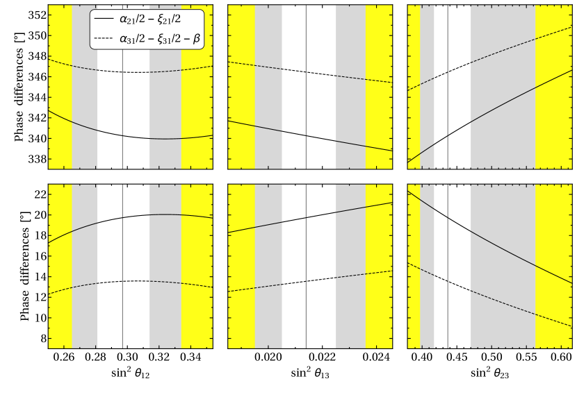
Figure 1: The phase differences $(\alpha_{21}/2-\xi_{21}/2)$ (solid line) and $(\alpha_{31}/2-\xi_{31}/2-\beta$) (dashed line) as functions of $\sin^{2}\theta_{ij}$ in case B1 and for the TBM symmetry form of the matrix $\tilde{U}_{\nu}$. The two other parameters, $\sin^{2}\theta_{kl}$ and $\sin^{2}\theta_{mn}$, $ij\neq kl\neq mn$, have been fixed to their best fit values for the NO spectrum. The upper panels correspond to $\delta=\cos^{-1}(\cos\delta)$, while the lower panels correspond to $\delta=2\pi-\cos^{-1}(\cos\delta)$. The vertical line and the three coloured vertical bands indicate the best fit value and the $1\sigma$, $2\sigma$ and $3\sigma$ allowed ranges of $\sin^{2}\theta_{ij}$.

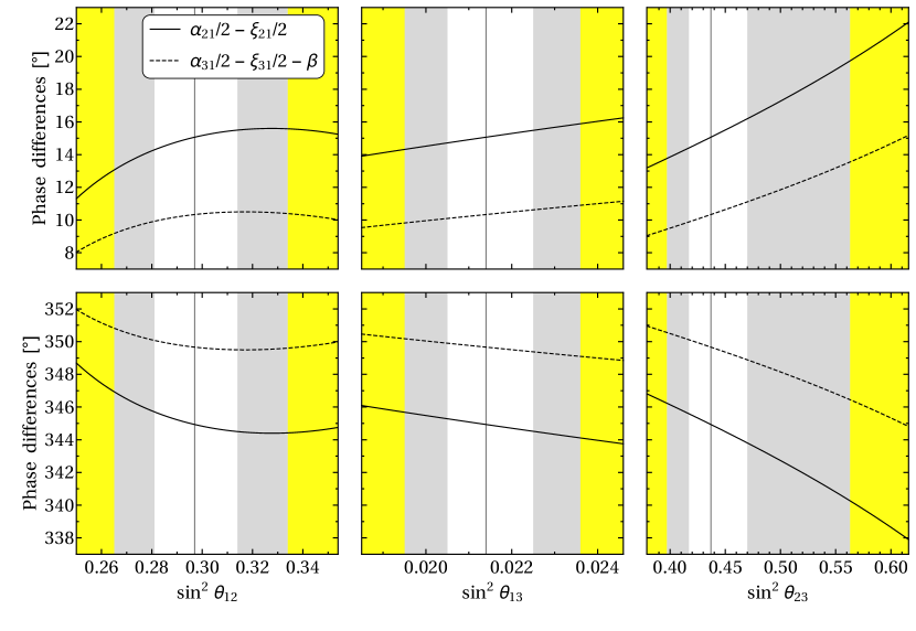
Figure 2: The same as in Fig. 1, but for case B2.

For a given symmetry form of $\tilde{U}_{\nu}$ — TBM, GRA, GRB and HG — the phase difference $(\alpha_{21}/2-\xi_{21}/2)$ has very similar values for the A1, B1 and B3 schemes, they differ approximately by at most $2^{\circ}$, and for the A2 and B2 schemes, for which the difference does not exceed $3^{\circ}$. However, the predictions for $(\alpha_{21}/2-\xi_{21}/2)$ for schemes A1, B1, B3 and A2, B2 differ significantly — the sum of the values of $(\alpha_{21}/2-\xi_{21}/2)$ for any of the A1, B1, B3 schemes and for any of the A2, B2 schemes being roughly equal to $2\pi$. In contrast, for a given symmetry form of $\tilde{U}_{\nu}$ — TBM, GRA, GRB and HG — i) the values of the phase difference $(\alpha_{31}/2-\xi_{31}/2)$ ($(\alpha_{31}/2-\xi_{31}/2-\beta)$) for the schemes A1 and A2 (B1 and B2) differ significantly — by up to $26^{\circ}$ ($337^{\circ}$), and ii) the values of $(\alpha_{31}/2-\xi_{31}/2)$ and $(\alpha_{31}/2-\xi_{31}/2-\beta)$ are drastically different. At the same time, the values of $(\alpha_{31}/2-\xi_{31}/2)$ for the A1 and B3 schemes practically coincide.

Finally, for any given of the five cases of schemes C1 and C2, the values of the phase difference $(\alpha_{21}/2-\xi_{21}/2)$ for schemes C1 and C2 differ drastically. The same conclusion is valid for the C1 and C2 values of the phase difference $(\alpha_{31}/2-\xi_{31}/2)$ for any of the first three cases of these schemes listed in Table 4. For the last two cases in Table 4 the difference between the C1 and C2 values of $(\alpha_{31}/2-\xi_{31}/2)$ is approximately $12^{\circ}$ and $18^{\circ}$.

Further, we show how the predictions for the phase differences presented in Tables 3 and 4 change when the uncertainties in determination of the neutrino mixing parameters are taken into account. As an example, we consider the cases B1 and B2 with the TBM form of the matrix $\tilde{U}_{\nu}$. We fix two of $\sin^{2}\theta_{ij}$ to their best fit values for the NO neutrino mass spectrum and vary the third one in its $3\sigma$ allowed range given in eqs. (3) – (5). We show the results for cases B1 and B2 in Figs. 1 and 2, respectively. As can be seen, the phase differences of interest depend weakly on $\sin^{2}\theta_{12}$ and $\sin^{2}\theta_{13}$. When these parameters are varied in their $3\sigma$ ranges, the variation of the phase differences is within a few degrees. The dependence on $\sin^{2}\theta_{23}$ is stronger: the maximal variations of $(\alpha_{21}/2-\xi_{21}/2)$ and $(\alpha_{31}/2-\xi_{31}/2-\beta)$ are approximately of $9^{\circ}$ and $6^{\circ}$ in both cases. Another example, corresponding to the cases A1 and A2 with the TBM form of the matrix $\tilde{U}_{\nu}$, is considered in Appendix A.

Performing a full statistical analysis of the predictions for $(\alpha_{21}/2-\xi_{21}/2)$ and $(\alpha_{31}/2-\xi_{31}/2)$ ($(\alpha_{31}/2-\xi_{31}/2-\beta)$) is however outside the scope of the present study. Such an analysis will be presented elsewhere.

6.3 Neutrinoless Double Beta Decay

If the light neutrinos with definite mass $\nu_{j}$ are Majorana fermions, their exchange can trigger processes in which the total lepton charge changes by two units, $|\Delta L|=2$: $K^{+}\rightarrow\pi^{-}+\mu^{+}+\mu^{+}$, $e^{-}+(A,Z)\rightarrow e^{+}+(A,Z-2)$, etc. The experimental searches for $(\beta\beta)_{0\nu}$-decay, $(A,Z)\rightarrow(A,Z+2)+e^{-}+e^{-}$, of even-even nuclei ${}^{48}Ca$, ${}^{76}Ge$, ${}^{82}Se$, ${}^{100}Mo$, ${}^{116}Cd$, ${}^{130}Te$, ${}^{136}Xe$, ${}^{150}Nd$, etc., are unique in reaching the sensitivity that might allow to observe this process if it is triggered by the exchange of the light neutrinos $\nu_{j}$ (see, e.g., refs. [14, 16]). In $(\beta\beta)_{0\nu}$-decay, two neutrons of the initial nucleus $(A,Z)$ transform by exchanging virtual $\nu_{1,2,3}$ into two protons of the final state nucleus $(A,Z+2)$ and two free electrons. The corresponding $(\beta\beta)_{0\nu}$-decay amplitude has the form (see, e.g., refs. [10, 16]): $A(\mbox{$(\beta\beta)_{0\nu}$})=G^{2}_{\rm F}\,\mbox{$\langle\!\,m\,\!\rangle$}\,M(A,Z)$, where $G_{\rm F}$ is the Fermi constant, $\langle\!\,m\,\!\rangle$ is the $(\beta\beta)_{0\nu}$-decay effective Majorana mass and $M(A,Z)$ is the nuclear matrix element (NME) of the process. The $(\beta\beta)_{0\nu}$-decay effective Majorana mass $\langle\!\,m\,\!\rangle$ contains all the dependence of $A(\mbox{$(\beta\beta)_{0\nu}$})$ on the neutrino mixing parameters. The current experimental limits on $\left|\langle\!\,m\,\!\rangle\right|$ are in the range of $(0.1-0.7)$ eV. Most importantly, a large number of experiments of a new generation aim at sensitivity to $\mbox{$\left|\langle\!\,m\,\!\rangle\right|$}\sim(0.01-0.05)$ eV (for a detailed discussion of the current limits on $\left|\langle\!\,m\,\!\rangle\right|$ and of the currently running and future planned $(\beta\beta)_{0\nu}$-decay experiments and their prospective sensitivities see, e.g., the recent review article [60]).

The predictions for $\left|\langle\!\,m\,\!\rangle\right|$ (see, e.g., [10, 15, 16]),

$$\left|\langle\!\,m\,\!\rangle\right| =\left|\sum_{i=1}^{3}m_{i}U_{ei}^{2}\right|$$

$$=\left|m_{1}\cos^{2}\theta_{12}\cos^{2}\theta_{13}+m_{2}\sin^{2}\theta_{12}\cos^{2}\theta_{13}e^{i\alpha_{21}}+m_{3}\sin^{2}\theta_{13}e^{i\left(\alpha_{31}-2\delta\right)}\right|\,,$$ (239)

$m_{1,2,3}$ being the light Majorana neutrino masses, depend on the values of the Majorana phase $\alpha_{21}$ and on the Majorana-Dirac phase difference $(\alpha_{31}-2\delta)$. In what follows we will derive predictions for $\left|\langle\!\,m\,\!\rangle\right|$ as a function of the lightest neutrino mass $m_{\rm min}\equiv{\rm min}(m_{j})$, $j=1,2,3$, for both the NO and IO neutrino mass spectra and for two values of each of the phases $\xi_{21}$ and $\xi_{31}$: $\xi_{21}=0$ or $\pi$, $\xi_{31}=0$ or $\pi$. The choice of the two values of the phases $\xi_{21}$ and $\xi_{31}$ will be justified in the next Section where we show that the requirement of generalised CP invariance of the neutrino Majorana mass term in the cases of the $S_{4}$, $A_{4}$, $T^{\prime}$ and $A_{5}$ lepton flavour symmetries leads to the constraints $\xi_{21}=0$ or $\pi$, $\xi_{31}=0$ or $\pi$.

We use the standard convention for numbering the neutrinos with definite masses in the cases of the NO and IO spectra (see, e.g., [1]): $m_{1}<m_{2}<m_{3}$ for the NO spectrum and $m_{3}<m_{1}<m_{2}$ for the IO one. We recall that the two heavier neutrino masses are expressed in terms of the lightest neutrino mass and the two independent neutrino mass squared differences measured in neutrino oscillation experiments as follows:

$$m_{2}=\sqrt{\Delta m^{2}_{21}+m^{2}_{1}}\,,\quad m_{3}=\sqrt{\Delta m^{2}_{31}+m^{2}_{1}}\quad{\rm for~{}the~{}NO~{}spectrum}\,,$$ (240)

$$m_{1}=\sqrt{\Delta m^{2}_{23}-\Delta m^{2}_{21}+m^{2}_{3}}\,,\quad m_{2}=\sqrt{\Delta m^{2}_{23}+m^{2}_{3}}\quad{\rm for~{}the~{}IO~{}spectrum}\,,$$ (241)

where $\Delta m^{2}_{ij}\equiv m^{2}_{i}-m^{2}_{j}$. The best fit values and the $3\sigma$ allowed ranges of $\Delta m^{2}_{21}$ and $\Delta m^{2}_{31(23)}$ obtained in the global analysis of the neutrino oscillation data performed in [24] we are going to use in our numerical study read:

$$(\Delta m^{2}_{21})_{\rm BF}=7.37\times 10^{-5}~{}\text{eV}^{2}\,,\quad 6.93\times 10^{-5}~{}\text{eV}^{2}\leq\Delta m^{2}_{21}\leq 7.97\times 10^{-5}~{}\text{eV}^{2}\,,$$ (242)

$$(\Delta m^{2}_{31(23)})_{\rm BF}=2.54~{}(2.50)\times 10^{-3}~{}\text{eV}^{2}\,,$$

$$2.40~{}(2.36)\times 10^{-3}~{}\text{eV}^{2}\leq\Delta m^{2}_{31(23)}\leq 2.67~{}(2.64)\times 10^{-3}~{}\text{eV}^{2}\,,$$ (243)

where the quoted values of $\Delta m^{2}_{31}$ and $\Delta m^{2}_{23}$ correspond to the NO and IO spectra, respectively.

As can be seen from Tables 2 – 4, the values of all three phases, $\delta$, $\alpha_{21}$ and $\alpha_{31}$, for scheme B3 with $\omega=0$ and ${\rm sgn}\,(\sin 2\theta^{e}_{13})=1$ are very close to the values for scheme A1. Thus, the predictions for $\left|\langle\!\,m\,\!\rangle\right|$ in scheme B3 are practically the same as those for scheme A1 and we present predictions only for the latter.

In Fig. 3 we show the absolute value of the effective Majorana mass $\left|\langle\!\,m\,\!\rangle\right|$ versus the lightest neutrino mass $m_{\rm min}$ in the cases of schemes A1, A2, B1, B2, C1 and C2 for the NO (blue lines and bands) and IO (dark-red lines and bands) neutrino mass spectra, using the best fit values of the mixing angles $\theta_{12}$ and $\theta_{13}$ quoted in eqs. (3) and (5), the best fit values of the two neutrino mass squared differences $\Delta m^{2}_{21}$ and $\Delta m^{2}_{31(23)}$ given in eqs. (242) and (243), the values of the Dirac phase $\delta$ from Table 2 and the values of the Majorana phases $\alpha_{21}$ and $\alpha_{31}$ extracted from Tables 3 and 4 setting $(\xi_{21},\xi_{31})=(0,0)$. In Figs. 4, 5 and 6 the values of $(\xi_{21},\xi_{31})$ are fixed to $(0,\pi)$, $(\pi,0)$ and $(\pi,\pi)$, respectively.

In cases A1 and A2 the solid blue line corresponds to the TBM symmetry form of the matrix $\tilde{U}_{\nu}$, while the medium, small and tiny dashed blue lines are for the GRB, GRA and HG symmetry forms, respectively. In cases B1 and B2 the predicted values of $\left|\langle\!\,m\,\!\rangle\right|$ for all the symmetry forms considered are within the blue and dark-red bands obtained varying the phase $\beta$ within the interval $[0,\pi]$. In case C1 (C2) the solid blue line stands for case I (II) characterised by $[\theta^{\nu}_{13},\theta^{\nu}_{12}]=[\pi/20,-\pi/4]$ ($[\pi/20,\pi/4]$), while the large, medium, small and tiny dashed blue lines are for cases V (III), II (V), IV (I) and III (IV), respectively, where the values of $[\theta^{\nu}_{13},\theta^{\nu}_{12}]$ in each of these cases are given in the text below Table 2.

The light-blue and light-red areas are obtained varying the neutrino oscillation parameters $\theta_{12}$, $\theta_{13}$, $\Delta m^{2}_{21}$ and $\Delta m^{2}_{31(23)}$ within their respective $3\sigma$ ranges quoted in eqs. (3), (5), (242) and (243), and the phases $\alpha_{21}$ and $(\alpha_{31}-2\delta)$ within the interval  $[0,2\pi]$. The horizontal grey band indicates the upper bound on $\left|\langle\!\,m\,\!\rangle\right|$ of $(0.2-0.4)$ eV obtained in [62]. The vertical dashed line represents the prospective upper limit on $m_{\rm min}$ of $0.2$ eV from the KATRIN experiment [63].

As Figs. 3 and 4 show, for $(\xi_{21},\xi_{31})=(0,0)$ and $(0,\pi)$, the absolute value of the effective Majorana mass $\left|\langle\!\,m\,\!\rangle\right|$ for the IO spectrum has practically the maximal possible values for all schemes considered. In the case of the NO spectrum and $(\xi_{21},\xi_{31})=(0,0)$, $\left|\langle\!\,m\,\!\rangle\right|$ is always bigger than $(1.5-2.0)\times 10^{-3}$ eV. For $(\xi_{21},\xi_{31})=(0,\pi)$, $\left|\langle\!\,m\,\!\rangle\right|$ has the maximal possible values in the A1 and A2 schemes as well in case I (II) of the C1 (C2) scheme; in the other cases of the C1 (C2) scheme, $\left|\langle\!\,m\,\!\rangle\right|$ is always bigger than $2.0\times 10^{-3}$ eV. In the B1 and B2 schemes and the NO spectrum, $\left|\langle\!\,m\,\!\rangle\right|$ can have the maximal possible values for both sets of values of $(\xi_{21},\xi_{31})=(0,0)$ and $(0,\pi)$.

For $(\xi_{21},\xi_{31})=(\pi,0)$ and $(\pi,\pi)$ (Figs. 5 and 6) and the IO spectrum, a partial compensation between the three terms in $\left|\langle\!\,m\,\!\rangle\right|$ takes place for all schemes considered. However, $\mbox{$\left|\langle\!\,m\,\!\rangle\right|$}\ \raisebox{-1.72218pt}{\hbox to0.0pt{$\sim$\hss}}\raisebox{1.72218pt}{$>$}\ 2\times 10^{-2}$ eV for all cases analysed by us. The mutual compensation between the different terms in $\left|\langle\!\,m\,\!\rangle\right|$ can be stronger in the case of the NO spectrum, when $\mbox{$\left|\langle\!\,m\,\!\rangle\right|$}\ \raisebox{-1.72218pt}{\hbox to0.0pt{$\sim$\hss}}\raisebox{1.72218pt}{$<$}\ 10^{-3}$ eV in certain cases in specific intervals of values of $m_{1}$, typically between approximately $10^{-3}$ eV and $7\times 10^{-3}$ eV.

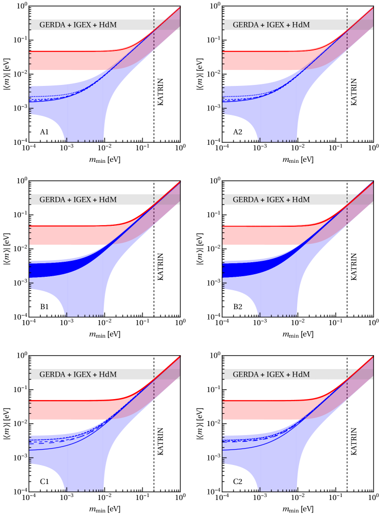
Figure 3: The absolute value of the effective Majorana mass $\left|\langle\!\,m\,\!\rangle\right|$ versus the lightest neutrino mass $m_{\rm min}$. The blue (dark-red) lines and bands correspond to $\left|\langle\!\,m\,\!\rangle\right|$ computed using the best fit values of $\theta_{12}$ and $\theta_{13}$ for the NO (IO) spectrum and the values of $\delta$, $\alpha_{21}$ and $\alpha_{31}$ obtained using the corresponding sum rules and assuming $(\xi_{21},\xi_{31})=(0,0)$. In cases A1 and A2 the solid blue line corresponds to the TBM symmetry form, while the medium, small and tiny dashed blue lines are for the GRB, GRA and HG symmetry forms, respectively. In cases B1 and B2 the predicted values of $\left|\langle\!\,m\,\!\rangle\right|$ for all the symmetry forms considered are within the blue and dark-red bands obtained varying the phase $\beta$ in the interval $[0,\pi]$. In case C1 (C2) the solid blue line stands for case I (II), while the large, medium, small and tiny dashed blue lines are for cases V (III), II (V), IV (I) and III (IV), respectively. The light-blue and light-red areas are obtained varying the neutrino oscillation parameters $\theta_{12}$, $\theta_{13}$, $\Delta m^{2}_{21}$ and $\Delta m^{2}_{31(23)}$ in their respective $3\sigma$ ranges quoted in eqs. (3), (5), (242) and (243) and the phases $\alpha_{21}$ and $(\alpha_{31}-2\delta)$ in the interval $[0,2\pi]$. The horizontal grey band indicates the upper bound $\mbox{$\left|\langle\!\,m\,\!\rangle\right|$}\sim 0.2-0.4$ eV obtained in [62]. The vertical dashed line represents the prospective upper limit on $m_{\rm min}$ of $0.2$ eV from the KATRIN experiment [63].

Figure 4: The same as in Fig. 3, but for $(\xi_{21},\xi_{31})=(0,\pi)$.

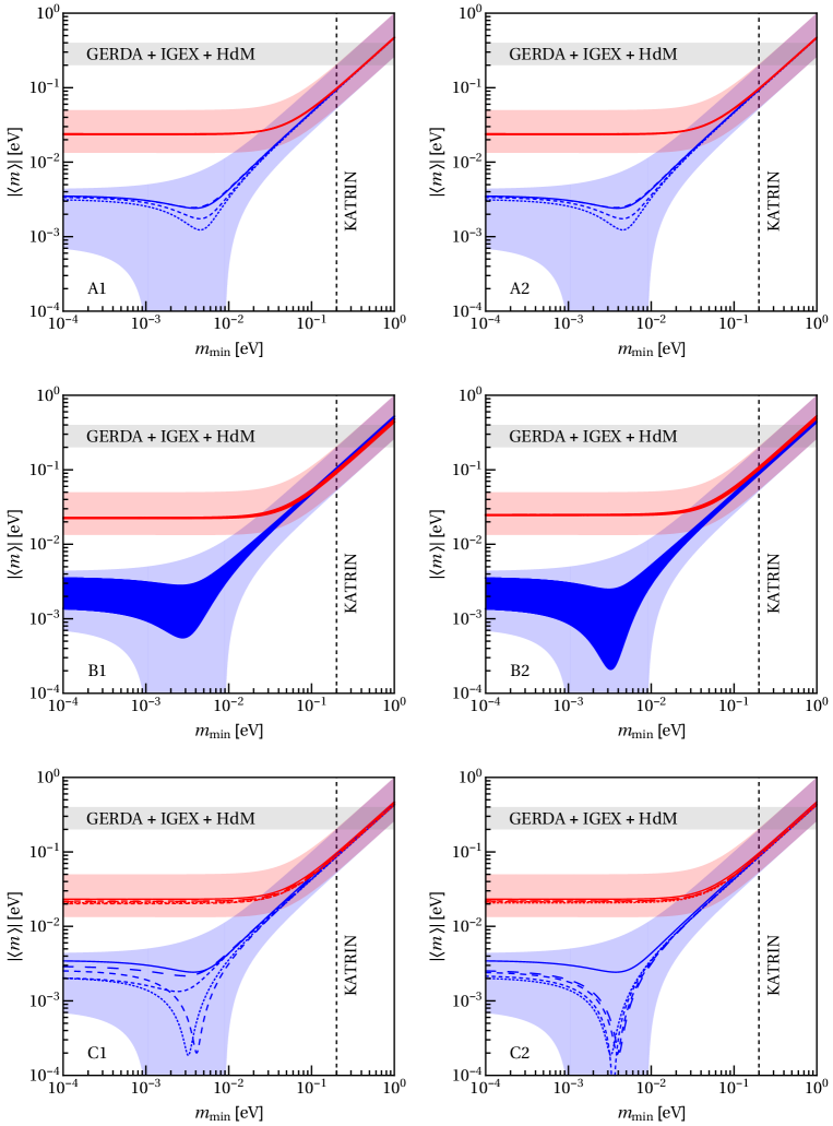
Figure 5: The same as in Fig. 3, but for $(\xi_{21},\xi_{31})=(\pi,0)$.

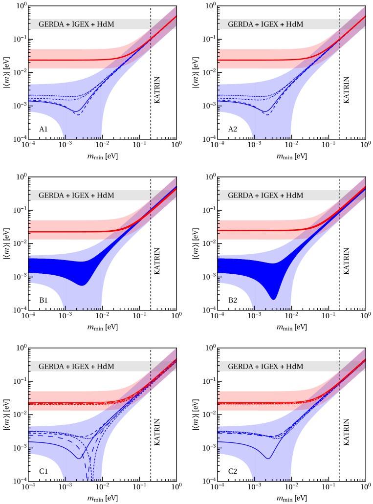
Figure 6: The same as in Fig. 3, but for $(\xi_{21},\xi_{31})=(\pi,\pi)$.

7 Implications of Generalised CP Symmetry Combined with Flavour Symmetry

In the present Section we derive constraints on the phases $\xi_{21}$ and $\xi_{31}$ in the matrix $U_{\nu}$, which diagonalises the neutrino Majorana mass matrix $M_{\nu}$, within the approach in which a lepton flavour symmetry $G_{f}$ is combined with a generalised CP symmetry $H_{\rm CP}$. We examine successively the cases of $G_{f}=A_{4}~{}(T^{\prime})$, $S_{4}$ and $A_{5}$ with the three LH charged leptons and three LH flavour neutrinos transforming under a 3-dimensional representation $\rho$ of $G_{f}$. At low energies the flavour symmetry $G_{f}$ has necessarily to be broken down to residual symmetries $G_{e}$ and $G_{\nu}$ in the charged lepton and neutrino sectors, respectively. All the cases considered in the present study fall into the class of residual symmetries with trivial $G_{e}$ ($G_{f}$ being fully broken in the charged lepton sector) and $G_{\nu}=Z_{2}\times Z_{2}$ .

The residual symmetry $G_{\nu}$ alone does not provide any information on the phases $\xi_{21}$ and $\xi_{31}$ of interest. Indeed, let $\bar{U}_{\nu}$ be a unitary matrix which diagonalises the complex symmetric neutrino Majorana mass matrix:

$$\bar{U}_{\nu}^{T}\,M_{\nu}\,\bar{U}_{\nu}=\operatorname{diag}\left(m_{1}e^{-i\xi_{1}},m_{2}e^{-i\xi_{2}},m_{3}e^{-i\xi_{3}}\right)\,,$$ (244)

where $m_{i}$ are non-negative non-degenerate masses  and $\xi_{i}$ are phases contributing to the Majorana phases in the PMNS matrix. Let us introduce the matrices

$$\bar{Q}_{0}=\operatorname{diag}\left(e^{i\frac{\xi_{1}}{2}},e^{i\frac{\xi_{2}}{2}},e^{i\frac{\xi_{3}}{2}}\right)\,,$$ (245)

and $U_{\nu}\equiv\bar{U}_{\nu}\bar{Q}_{0}$, such that

$$U_{\nu}^{T}\,M_{\nu}\,U_{\nu}=M_{\nu}^{\rm d}\equiv\operatorname{diag}\left(m_{1},m_{2},m_{3}\right)\,.$$ (246)

Thus,

$$U_{\nu}=\bar{U}_{\nu}\,\bar{Q}_{0}=e^{i\frac{\xi_{1}}{2}}\Psi_{\nu}\tilde{U}_{\nu}\,Q_{0}\,,$$ (247)

where $\Psi_{\nu}$ is a diagonal phase matrix containing, in general, two phases, $\xi_{1}/2$ is a common unphysical phase, and

$$Q_{0}={\rm diag}\left(1,e^{i\frac{\xi_{2}-\xi_{1}}{2}},e^{i\frac{\xi_{3}-\xi_{1}}{2}}\right)={\rm diag}\left(1,e^{i\frac{\xi_{21}}{2}},e^{i\frac{\xi_{31}}{2}}\right)\,.$$ (248)

Clearly, the phases of interest are $\xi_{21}=\xi_{2}-\xi_{1}$ and $\xi_{31}=\xi_{3}-\xi_{1}$. It is clear from eq. (247) that the common phases of the columns of $U_{\nu}$ have been factorised in the matrix $\bar{Q}_{0}$.

The $G_{\nu}$ invariance of the neutrino mass matrix implies

$$\rho(g_{\nu})^{T}\,M_{\nu}\,\rho(g_{\nu})=M_{\nu}\quad\forall\,g_{\nu}\in G_{\nu}\,.$$ (249)

Further, using eq. (246), we find

$$(\rho^{({\rm d})}(g_{\nu}))^{T}\,M_{\nu}^{\rm d}\,\rho^{({\rm d})}(g_{\nu})=M_{\nu}^{\rm d}\,,\quad\text{with}\quad\rho^{({\rm d})}(g_{\nu})=U_{\nu}^{\dagger}\,\rho(g_{\nu})\,U_{\nu}\,.$$ (250)

For $m_{1}\neq m_{2}\neq m_{3}$ and ${\rm min}(m_{j})\neq 0$, $j=1,2,3$, as it is not difficult to show, the matrix $\rho^{({\rm d})}(g_{\nu})$ can have only the following form:

$$\rho^{({\rm d})}(g_{\nu})=\operatorname{diag}(\pm 1,\pm 1,\pm 1)\,,$$ (251)

where the signs of the three non-zero entries in $\rho^{({\rm d})}(g_{\nu})$ are not correlated. Finally, from the preceding two equations we get

$$\rho^{({\rm d})}(g_{\nu})=\bar{Q}_{0}\,\rho^{({\rm d})}(g_{\nu})\,\bar{Q}_{0}^{*}=\bar{U}_{\nu}^{\dagger}\,\rho(g_{\nu})\,\bar{U}_{\nu}\,,$$ (252)

i.e., the phases $\xi_{i}$ cancel out. Therefore a lepton flavour symmetry alone does not lead to any constraints on the phases $\xi_{i}$, $i=1,2,3$, and thus on the phases $\xi_{21}$ and $\xi_{31}$.

Let us consider next the implications of a residual generalised CP symmetry $H_{\rm CP}^{\nu}\subset H_{\rm CP}$, which is preserved in the neutrino sector. In this case the neutrino Majorana mass matrix satisfies the following condition:

$$X_{i}^{T}\,M_{\nu}\,X_{i}=M_{\nu}^{*}\,,$$ (253)

where $X_{i}\in H_{\rm CP}^{\nu}$ are the generalised CP transformations. Substituting $M_{\nu}$ from eq. (246), we find

$$(X_{i}^{\rm d})^{T}\,M_{\nu}^{\rm d}\,X_{i}^{\rm d}=M_{\nu}^{\rm d}\,,\quad\text{with}\quad X_{i}^{\rm d}=U_{\nu}^{\dagger}\,X_{i}\,U_{\nu}^{*}\,.$$ (254)

Again, since the three neutrino masses in $M_{\nu}^{\rm d}$ have to be, as it follows from the data, non-degenerate, we have

$$X_{i}^{\rm d}=\operatorname{diag}(\pm 1,\pm 1,\pm 1)\,.$$ (255)

Finally, using that $U_{\nu}\equiv\bar{U}_{\nu}\bar{Q}_{0}$, we obtain [65]

$$\operatorname{diag}\left(\pm e^{i\xi_{1}},\pm e^{i\xi_{2}},\pm e^{i\xi_{3}}\right)=\bar{Q}_{0}\,X_{i}^{\rm d}\,\bar{Q}_{0}=\bar{U}_{\nu}^{\dagger}\,X_{i}\,\bar{U}_{\nu}^{*}\,.$$ (256)

Thus, we come to the conclusion that the phases $\xi_{i}$ will be known once i) the matrix $\bar{U}_{\nu}$ is fixed by the residual flavour symmetry $G_{\nu}$, and ii) the generalised CP transformations $X_{i}\in H_{\rm CP}^{\nu}$, which are consistent with $G_{\nu}$, are identified.

Now we turn to concrete examples. For $G_{f}=A_{4}$ we choose to work in the Altarelli-Feruglio basis [66]. Preserving the $S$ generator leads to $\bar{U}_{\nu}=U_{\rm TBM}$, provided there is an additional accidental $\mu$ – $\tau$ symmetry [38]. Then, twelve generalised CP transformations consistent with the $A_{4}$ flavour symmetry for the triplet representation in the chosen basis have been found in [67], solving the consistency condition

$$X\,\rho^{*}(g)\,X^{-1}=\rho(g^{\prime})\,,\quad g,g^{\prime}\in A_{4}\,.$$ (257)

These transformations can be summarised in a compact way as follows:

$$X=\rho(g)\,,\quad g\in A_{4}\,,$$ (258)

i.e., the generalised CP transformations consistent with the $A_{4}$ flavour symmetry are of the same form as the flavour symmetry group transformations [67]. They are given in Table 1 in [67] together with the elements $\hat{S}$ and $\hat{T}$ to which the generators $S$ and $T$ of $A_{4}$ are mapped by the consistency condition in eq. (257). Further, since in our case the residual flavour symmetry $G_{\nu}=Z_{2}\times Z_{2}$, where one $Z_{2}$ factor corresponds to the preserved $S$ generator, only those $X$ are acceptable, for which $\hat{S}=S$. From Table 1 in [67] it follows that there are four such generalised CP transformations, namely, $\rho(E)$, $\rho(S)$, $\rho(T^{2}ST)$ and $\rho(TST^{2})$, where $E$ is the identity element of the group. The last two transformations are not symmetric in the chosen basis, and, as shown in [67], lead to partially degenerate neutrino mass spectrum with two equal masses (see also [53]), which is ruled out by the existing neutrino oscillation data. Thus, we are left with two allowed generalised CP transformations, $\rho(E)$ and $\rho(S)$, for which we have:

$$U_{\rm TBM}^{\dagger}\,\rho(E)\,U^{*}_{\rm TBM}=\rho(E)=\operatorname{diag}(1,1,1)\,,$$ (259)

$$U_{\rm TBM}^{\dagger}\,\rho(S)\,U^{*}_{\rm TBM}=\operatorname{diag}(-1,1,-1)\,.$$ (260)

Finally, according to eq. (256), this implies that the phases $\xi_{i}$ can be either $0$ or $\pi$. The same conclusion holds for a $T^{\prime}$ flavour symmetry, because restricting ourselves to the triplet representation for the LH charged lepton and neutrino fields, there is no way to distinguish $T^{\prime}$ from $A_{4}$ [39].

In the case of $G_{f}=S_{4}$ we choose to work in the basis given in [40]. The residual symmetry $G_{\nu}=Z_{2}\times Z_{2}$, where one $Z_{2}$ factor corresponds to preserved $S$ generator in the chosen basis and the second one arises accidentally (a $\mu$ – $\tau$ symmetry), leads to $\bar{U}_{\nu}=U_{\rm BM}$ [40]. As in the previous example, the generalised CP transformations consistent with the $S_{4}$ flavour symmetry are of the same form as the flavour symmetry group transformations [54]. Solving the consistency condition in eq. (257), we find ten symmetric generalised CP transformations consistent with the $S_{4}$ flavour symmetry for the triplet representation in the chosen basis. We summarise them in Table 5 together with elements $\hat{T}$ and $\hat{S}$ to which the consistency condition maps the group generators $T$ and $S$.

$g$, $X=\rho(g)$	$T\rightarrow\hat{T}$	$S\rightarrow\hat{S}$
$(ST^{2})^{2}$	$T$	$S$
$T^{3}$	$T^{3}$	$T^{3}ST$
$E$	$T^{3}$	$S$
$T$	$T^{3}$	$TST^{3}$
$T^{2}ST^{2}$	$STS$	$S$
$ST^{2}S$	$T$	$T^{2}ST^{2}$
$S$	$TST$	$S$
$T^{2}$	$T^{3}$	$T^{2}ST^{2}$
$STS$	$ST^{2}$	$ST^{2}ST$
$TST$	$T^{2}S$	$TST^{2}S$

Table 5: The ten symmetric generalised CP transformations $X=\rho(g)$ consistent with the $S_{4}$ flavour symmetry for the triplet representation $\rho$ in the chosen basis [40] determined by the consistency condition in eq. (257). The mapping $(T,S)\rightarrow(\hat{T},\hat{S})$ is realised via the consistency condition applied to the group generators $T$ and $S$, i.e., $X\rho^{*}(T)X^{-1}=\rho(\hat{T})$ and $X\rho^{*}(S)X^{-1}=\rho(\hat{S})$.

From this table we see that there are four symmetric generalised CP transformations consistent with the preserved $S$ generator, namely, $\rho(E)$, $\rho(S)$, $\rho(T^{2}ST^{2})$ and $\rho(ST^{2}ST^{2})$. Substituting them and $\bar{U}_{\nu}=U_{\rm BM}$ in eq. (256), we find:

$$U_{\rm BM}^{\dagger}\,\rho(E)\,U^{*}_{\rm BM}=\rho(E)=\operatorname{diag}(1,1,1)\,,$$ (261)

$$U_{\rm BM}^{\dagger}\,\rho(S)\,U^{*}_{\rm BM}=\operatorname{diag}(1,-1,1)\,,$$ (262)

$$U_{\rm BM}^{\dagger}\,\rho(T^{2}ST^{2})\,U^{*}_{\rm BM}=\operatorname{diag}(-1,1,1)\,,$$ (263)

$$U_{\rm BM}^{\dagger}\,\rho(ST^{2}ST^{2})\,U^{*}_{\rm BM}=\operatorname{diag}(-1,-1,1)\,.$$ (264)

Therefore also in this case the phases $\xi_{i}$ are fixed by residual generalised CP symmetry to be either $0$ or $\pi$.

As a third example, we consider $G_{f}=A_{5}$. We employ the basis for the triplet representation of the generators $S$ and $T$ of this group given in [68]. The residual symmetry $G_{\nu}=Z_{2}\times Z_{2}$ generated by $S$ and $T^{3}ST^{2}ST^{3}$ leads to GRA mixing, i.e., $\bar{U}_{\nu}=U_{\rm GRA}$, as is shown in [68]. It is stated in [69] that the generalised CP transformations consistent with $A_{5}$ are of the same form as the group transformations. Solving the consistency condition in eq. (257), we find 16 symmetric generalised CP transformations consistent with $A_{5}$ for the triplet representation in the working basis. We summarise them in Table 6, where we present also the elements $\hat{T}$ and $\hat{S}$.

$g$, $X=\rho(g)$	$T\rightarrow\hat{T}$	$S\rightarrow\hat{S}$
$T^{3}ST^{2}ST^{3}$	$STS$	$S$
$S$	$TST$	$S$
$(ST^{2})^{2}S$	$ST^{3}$	$(T^{2}S)^{2}T^{4}$
$TST$	$T^{2}S$	$TST^{2}S$
$ST^{3}S$	$T^{2}ST$	$ST^{3}ST^{2}S$
$T^{3}ST^{3}$	$T^{4}ST^{3}$	$T^{2}ST^{2}ST^{3}S$
$T^{3}ST^{2}ST^{3}S$	$T$	$S$
$T$	$T^{4}$	$TST^{4}$
$T^{2}$	$T^{4}$	$T^{2}ST^{3}$
$E$	$T^{4}$	$S$
$T^{3}$	$T^{4}$	$T^{3}ST^{2}$
$T^{4}$	$T^{4}$	$T^{4}ST$
$ST^{2}S$	$TST^{2}$	$ST^{2}ST^{3}S$
$T^{2}ST^{2}$	$T^{3}ST^{4}$	$T^{4}ST^{2}ST^{3}S$
$STS$	$ST^{2}$	$ST^{2}ST$
$(T^{2}S)^{2}T^{2}$	$T^{3}S$	$T^{4}(ST^{2})^{2}$

Table 6: The 16 symmetric generalised CP transformations $X=\rho(g)$ consistent with the $A_{5}$ flavour symmetry for the triplet representation $\rho$ in the chosen basis [68] determined by the consistency condition in eq. (257). The mapping $(T,S)\rightarrow(\hat{T},\hat{S})$ is realised via the consistency condition applied to the group generators $T$ and $S$, i.e., $X\rho^{*}(T)X^{-1}=\rho(\hat{T})$ and $X\rho^{*}(S)X^{-1}=\rho(\hat{S})$.

It follows from this table that the generalised CP transformations consistent with $G_{\nu}=Z_{2}\times Z_{2}$ of interest are of the same form of $G_{\nu}$. Namely, they are $\rho(E)$, $\rho(S)$, $\rho(T^{3}ST^{2}ST^{3})$ and $\rho(T^{3}ST^{2}ST^{3}S)$, and we have:

$$U_{\rm GRA}^{\dagger}\,\rho(E)\,U^{*}_{\rm GRA}=\rho(E)=\operatorname{diag}(1,1,1)\,,$$ (265)

$$U_{\rm GRA}^{\dagger}\,\rho(S)\,U^{*}_{\rm GRA}=\operatorname{diag}(1,-1,-1)\,,$$ (266)

$$U_{\rm GRA}^{\dagger}\,\rho(T^{3}ST^{2}ST^{3})\,U^{*}_{\rm GRA}=\operatorname{diag}(-1,1,-1)\,,$$ (267)

$$U_{\rm GRA}^{\dagger}\,\rho(T^{3}ST^{2}ST^{3}S)\,U^{*}_{\rm GRA}=\operatorname{diag}(-1,-1,1)\,.$$ (268)

Thus, as in the previous cases, the phases $\xi_{i}$ are fixed by generalised CP symmetry to be either $0$ or $\pi$.

It follows from the results derived in the present Section that the two phases $\xi_{21}=\xi_{2}-\xi_{1}$ and $\xi_{31}=\xi_{3}-\xi_{1}$, present in the matrix $Q_{0}$ (see eq. (9)) and giving contributions to the Majorana phases $\alpha_{21}$ and $\alpha_{31}$ in the PMNS matrix, are constrained to be either $0$ or $\pi$ for all examples considered.

Finally, we note that although in the cases of the flavour symmetry groups considered — $A_{4}$, $T^{\prime}$, $S_{4}$ and $A_{5}$ — we choose to work in specific basis for the generators of each symmetry group, the results on the phases $\xi_{1,2,3}$ we have obtained, as we show below, are basis-independent. Indeed, let $B$ be a unitary matrix, which realises the change of basis. Then, the representation matrices of the group elements in the new basis, $\tilde{\rho}(g)$, are given by

$$\tilde{\rho}(g)=B\,\rho(g)\,B^{\dagger}\,,\quad g\in G_{f}\,.$$ (269)

Expressing $\rho(g)$ from this equation and substituting it in the consistency condition given in eq. (257) leads to

$$\tilde{X}\,\tilde{\rho}^{*}(g)\,\tilde{X}^{-1}=\tilde{\rho}(g^{\prime})\,,\quad g,g^{\prime}\in G_{f}\,,$$ (270)

where

$$\tilde{X}=B\,X\,B^{T}$$ (271)

are the generalised CP transformations in the new basis. Now we substitute $X$ from this equation in eq. (256) and obtain

$$\left(\tilde{\bar{U}}_{\nu}\right)^{\dagger}\,\tilde{X}_{i}\,\left(\tilde{\bar{U}}_{\nu}\right)^{*}=\bar{U}_{\nu}^{\dagger}\,X_{i}\,\bar{U}_{\nu}^{*}=\operatorname{diag}\left(\pm e^{i\xi_{1}},\pm e^{i\xi_{2}},\pm e^{i\xi_{3}}\right)\,,$$ (272)

where $\tilde{\bar{U}}_{\nu}=B\,\bar{U}_{\nu}$ is the matrix which diagonalises the neutrino Majorana mass matrix $\tilde{M}_{\nu}$, $\tilde{M}_{\nu}=B^{*}M_{\nu}\,B^{\dagger}$, in the new basis, i.e.,

$$\tilde{\bar{U}}_{\nu}^{T}\,\tilde{M}_{\nu}\,\tilde{\bar{U}}_{\nu}=\bar{U}_{\nu}^{T}\,M_{\nu}\,\bar{U}_{\nu}=\operatorname{diag}\left(m_{1}e^{-i\xi_{1}},m_{2}e^{-i\xi_{2}},m_{3}e^{-i\xi_{3}}\right)\,.$$ (273)

What concerns the charged lepton sector, in all cases we consider in the present study a flavour symmetry $G_{f}$ is completely broken in the charged lepton sector, i.e., the residual symmetry group $G_{e}$ consists only of the identity element $E$. The change of basis yields $\tilde{\rho}(E)=B\,\rho(E)\,B^{\dagger}$. As can be easily shown, the matrix $U_{e}^{\prime}=B\,U_{e}$ diagonalises the hermitian matrix $\tilde{M}_{e}\,\tilde{M}_{e}^{\dagger}$, $\tilde{M}_{e}\,\tilde{M}_{e}^{\dagger}=B\,M_{e}\,M_{e}\,B^{\dagger}$, in the new basis, $M_{e}$ being the charged lepton mass matrix in the initial basis. Namely,

$${U_{e}^{\prime}}^{\dagger}\,\tilde{M}_{e}\,\tilde{M}_{e}^{\dagger}\,U_{e}^{\prime}=U_{e}^{\dagger}\,M_{e}\,M_{e}^{\dagger}\,U_{e}=\operatorname{diag}\left(m_{e}^{2},m_{\mu}^{2},m_{\tau}^{2}\right)\,.$$ (274)

Taking into account that $U_{\nu}^{\prime}=B\,U_{\nu}=B\,\bar{U}_{\nu}\,\bar{Q}_{0}$, we obtain for the PMNS matrix $U$:

$$U={U_{e}^{\prime}}^{\dagger}\,U_{\nu}^{\prime}=U_{e}^{\dagger}\,U_{\nu}=U_{e}^{\dagger}\,\bar{U}_{\nu}\,\bar{Q}_{0}\,.$$ (275)

Thus, as eqs. (272) and (275) demonstrate, the results for the phases $\xi_{i}$ are basis-independent.

8 Summary and Conclusions

In the present article we have obtained predictions for the Majorana phases $\alpha_{21}/2$ and $\alpha_{31}/2$ of the $3\times 3$ unitary neutrino mixing matrix $U=U_{e}^{\dagger}\,U_{\nu}=(\tilde{U}_{e})^{\dagger}\,\Psi\tilde{U}_{\nu}\,Q_{0}\,$, $U_{e}$ ($\tilde{U}_{e}$) and $U_{\nu}$ ($\tilde{U}_{\nu}$) being $3\times 3$ unitary (CKM-like) matrices arising from the diagonalisation respectively of the charged lepton and neutrino Majorana mass terms. Each of the diagonal phase matrices $\Psi$ and $Q_{0}$ contains, in general, two physical CPV phases [28]. The phases in the matrix $Q_{0}$, $\xi_{21}/2$ and $\xi_{31}/2$, contribute to the Majorana phases in the PMNS matrix. Our study employs a method proposed in [2] and is a natural continuation of the studies performed in [2, 3, 4]. We have considered forms of $\tilde{U}_{e}$ and $\tilde{U}_{\nu}$, permitting to express $\delta$ as a function of the PMNS mixing angles, $\theta_{12}$, $\theta_{13}$ and $\theta_{23}$, present in $U$, and the angles contained in $\tilde{U}_{\nu}$ [2, 4]. As we have shown, for the same forms, the Majorana phases $\alpha_{21}/2$ and $\alpha_{31}/2$ are determined by the values of $\theta_{12}$, $\theta_{13}$ and $\theta_{23}$ and the phases $\xi_{21}/2$ and $\xi_{31}/2$ (see below). We have derived such sum rules for $\alpha_{21}/2$ and $\alpha_{31}/2$ in the following cases:

• $U=R_{12}(\theta^{e}_{12})\Psi R_{23}(\theta^{\nu}_{23})R_{12}(\theta^{\nu}_{12})Q_{0}$ (case A1),

• $U=R_{13}(\theta^{e}_{13})\Psi R_{23}(\theta^{\nu}_{23})R_{12}(\theta^{\nu}_{12})Q_{0}$ (case A2),

• $U=R_{12}(\theta^{e}_{12})R_{23}(\theta^{e}_{23})\Psi R_{23}(\theta^{\nu}_{23})R_{12}(\theta^{\nu}_{12})Q_{0}$ (case B1),

• $U=R_{13}(\theta^{e}_{13})R_{23}(\theta^{e}_{23})\Psi R_{23}(\theta^{\nu}_{23})R_{12}(\theta^{\nu}_{12})Q_{0}$ (case B2),

• $U=R_{12}(\theta^{e}_{12})R_{13}(\theta^{e}_{13})\Psi R_{23}(\theta^{\nu}_{23})R_{12}(\theta^{\nu}_{12})Q_{0}$ (case B3),

• $U=R_{12}(\theta^{e}_{12})\Psi R_{23}(\theta^{\nu}_{23})R_{13}(\theta^{\nu}_{13})R_{12}(\theta^{\nu}_{12})Q_{0}$ (case C1),

• $U=R_{13}(\theta^{e}_{13})\Psi R_{23}(\theta^{\nu}_{23})R_{13}(\theta^{\nu}_{13})R_{12}(\theta^{\nu}_{12})Q_{0}$ (case C2),

where $R_{ij}$ are real matrices, $R^{T}=R^{-1}$, and $\theta^{e}_{ij}$ and $\theta^{\nu}_{ij}$ denote the rotation angles in $\tilde{U}_{e}$ and $\tilde{U}_{\nu}$, respectively. The sum rules are summarised in Section 5. In the sum rules, $\alpha_{21}/2$ and $\alpha_{31}/2$ are expressed, in general, in terms of the three measured angles of the PMNS matrix, $\theta_{12}$, $\theta_{13}$ and $\theta_{23}$, the phases $\xi_{21}/2$ and $\xi_{31}/2$ of the matrix $Q_{0}$, and the angles in $\tilde{U}_{\nu}$, which are supposed to have known values, determined by symmetries. In the cases of schemes B1 and B2 (scheme B3), $\alpha_{31}/2$ ($\delta$, $\alpha_{21}/2$ and $\alpha_{31}/2$) depends (depend) on one additional, in general, unknown phase $\beta$ ($\omega$), whose value can only be fixed in a self-consistent theory of generation of neutrino masses and mixing.

In order to obtain predictions for the Majorana phases one has to specify, in particular, the values of the angles in the matrix $\tilde{U}_{\nu}$. In the present study we have considered the following symmetry forms of $\tilde{U}_{\nu}$: tri-bimaximal (TBM), bimaximal (BM), golden ratio A (GRA), golden ratio B (GRB), and hexagonal (HG). All these forms are characterised by the same $\theta^{\nu}_{23}=-\pi/4$ and $\theta^{\nu}_{13}=0$, but differ by the value of the angle $\theta^{\nu}_{12}$. For the forms cited above and used in the present study the values of $\theta^{\nu}_{12}$ are given in the Introduction. In schemes C1 and C2 we have employed three representative fixed values of $\theta^{\nu}_{13}\neq 0$ considered in the literature and appearing in models with flavour symmetries, $\theta^{\nu}_{13}=\pi/20,~{}\pi/10$ and $\sin^{-1}(1/3)$, together with certain fixed values of $\theta^{\nu}_{12}$ — in total five different pairs of values of $[\theta^{\nu}_{13},\theta^{\nu}_{12}]$ in each of the two schemes. The values of the five pairs are given in Table 2.

Thus, for the specific symmetry forms of $\tilde{U}_{\nu}$ listed above and used in our numerical analysis, the phase differences a) $(\alpha_{21}/2-\xi_{21}/2)$ and $(\alpha_{31}/2-\xi_{31}/2)$ in schemes A1, A2, C1 and C2, b) $(\alpha_{21}/2-\xi_{21}/2)$ and $(\alpha_{31}/2-\xi_{31}/-\beta)$ in schemes B1 and B2, and c) $(\alpha_{21}/2-\xi_{21}/2)$ and $(\alpha_{31}/2-\xi_{31}/2)$ for a fixed $\omega$ in scheme B3, are determined completely by the values of the measured neutrino mixing angles $\theta_{12}$, $\theta_{13}$ and $\theta_{23}$ and the angles in the matrix $\tilde{U}_{\nu}$. If the value of the Dirac phase $\delta$ is measured, that will allow to fix the value of $\omega$ in scheme B3. Using the best fit values of $\theta_{12}$, $\theta_{13}$ and $\theta_{23}$, we have obtained predictions for the phase differences listed above, which are summarised in Tables 3 and 4. In the case of scheme B3, we have set $\omega=0$. For this value of $\omega$ the predicted value of the Dirac phase $\delta$ lies in the $2\sigma$ interval of allowed values quoted in eq. (6). The results reported in Tables 3 and 4 show that the phase differences of interest involving the Majorana phases $\alpha_{21}/2$ and $\alpha_{31}/2$ are determined with a two-fold ambiguity by the values of $\theta_{12}$, $\theta_{13}$ and $\theta_{23}$. This is a consequence of the fact that, as long as the sign of $\sin\delta$ is not fixed by the data, the Dirac phase $\delta$, on which the phase differences under discussion depend, is determined by the values of $\theta_{12}$, $\theta_{13}$ and $\theta_{23}$ in the schemes studied by us with a two-fold ambiguity [2, 3, 4], as Table 2 also shows. It follows from eq. (6) that the current data appear to favour negative values of $\sin\delta$. The predictions for the BM (LC) symmetry form of $\tilde{U}_{\nu}$ in Tables 3 and 4 correspond to the current $3\sigma$ upper bound of allowed values of $\sin^{2}\theta_{12}=0.354$ and the best fit values of $\sin^{2}\theta_{23}$ and $\sin^{2}\theta_{13}$, since using the best fit values of the three neutrino mixing angles one gets unphysical values of $|\cos\delta|>1$ [6, 2, 4]. Physical values of $\cos\delta$ are found for larger (smaller) values of $\sin^{2}\theta_{12}$ ($\sin^{2}\theta_{23}$) [2, 3, 4]. For $\sin^{2}\theta_{12}=0.354$ and the best fit values of $\sin^{2}\theta_{23}$ and $\sin^{2}\theta_{13}$, $|\cos\delta|$ has an unphysical value greater than one only for schemes B1 with the IO spectrum, B2 with the NO spectrum and B3, and for these cases we do not present results for the relevant phase differences.

We have investigated also how the predictions for the phase differences $(\alpha_{21}/2-\xi_{21}/2)$ and $(\alpha_{31}/2-\xi_{31}/2)$ ($(\alpha_{31}/2-\xi_{31}/2-\beta)$) presented in Tables 3 and 4 change when the uncertainties in determination of the neutrino mixing parameters are taken into account (see Figs. 1 and 2 and the related discussion as well as Appendix A).

Extracting the values of the Majorana phases $\alpha_{21}/2$ and $\alpha_{31}/2$ from the results presented in Tables 3 and 4 for two fixed values of each of the phases $\xi_{21}$ and $\xi_{31}$, $\xi_{21}=0$ and $\pi$, $\xi_{31}=0$ and $\pi$ (altogether four cases), and using also the predicted values of the Dirac phase $\delta$ from Table 2 and the best fit values of $\sin^{2}\theta_{12}$, $\sin^{2}\theta_{23}$ and $\sin^{2}\theta_{13}$, we derived (in graphic form) predictions for the absolute value of the neutrinoless double beta decay effective Majorana mass $\left|\langle\!\,m\,\!\rangle\right|$ as a function of the lightest neutrino mass $m_{\rm min}\equiv{\rm min}(m_{j})$, $j=1,2,3$, for both the NO and IO neutrino mass spectra (Figs. 3 – 6). For schemes B1 and B2 the predictions are obtained by varying the phase $\beta$ in the interval $[0,\pi]$. As a possible justification of the choice of the two values of the phases $\xi_{21}$ and $\xi_{31}$ used for the predictions of $\left|\langle\!\,m\,\!\rangle\right|$, we show that the requirement of generalised CP invariance of the neutrino Majorana mass term in the cases of the $S_{4}$, $A_{4}$, $T^{\prime}$ and $A_{5}$ lepton flavour symmetries leads to the constraints $\xi_{21}=0$ or $\pi$, $\xi_{31}=0$ or $\pi$.

The results derived in the present article for the Majorana CPV phases in the PMNS neutrino mixing matrix $U$ complement the results obtained in [2, 3, 4] on the predictions for the Dirac phase $\delta$ in $U$ in schemes in which the underlying form of $U$ is determined by, or is associated with, in particular, discrete (lepton) flavour symmetries.

Appendix A Impact of the $\boldsymbol{\sin^{2}\theta_{ij}}$ Uncertainties in Cases A1 and A2

In this Appendix we illustrate the impact of the uncertainties in determination of the neutrino mixing parameters on the predictions for the phase differences $(\alpha_{21}/2-\xi_{21}/2)$ and $(\alpha_{31}/2-\xi_{31}/2)$ in cases A1 and A2 with the TBM symmetry form of the matrix $\tilde{U}_{\nu}$. In Fig. 7 we show the dependence of $(\alpha_{21}/2-\xi_{21}/2)$ and $(\alpha_{31}/2-\xi_{31}/2)$ on $\sin^{2}\theta_{12}$ ($\sin^{2}\theta_{13}$) in case A1, fixing $\sin^{2}\theta_{13}$ ($\sin^{2}\theta_{12}$) to its best fit value for the NO spectrum. We recall that in this setup $\sin^{2}\theta_{23}$ is correlated with $\sin^{2}\theta_{13}$ by eq. (24) and, hence, is not a free parameter. In Fig. 8 we present results for case A2. Also in this scheme $\sin^{2}\theta_{23}$ is correlated with $\sin^{2}\theta_{13}$ and is not a free parameter (see eq. (50)). As can be seen from Figs. 7 and 8, in both cases A1 and A2 the variation of $(\alpha_{21}/2-\xi_{21}/2)$ is within $3^{\circ}$, while that of $(\alpha_{31}/2-\xi_{31}/2)$ is within $2^{\circ}$.

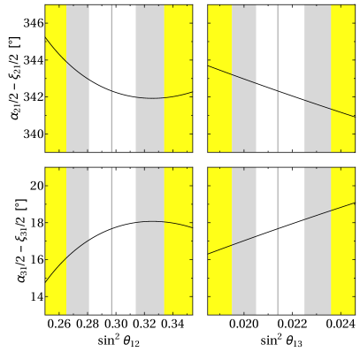
Figure 7: The phase differences $(\alpha_{21(31)}/2-\xi_{21(31)}/2)$ as functions of $\sin^{2}\theta_{12(13)}$ in case A1 and for the TBM form of the matrix $\tilde{U}_{\nu}$, fixing $\sin^{2}\theta_{13(12)}$ to its best fit value for the NO spectrum. The upper panels correspond to $\delta=\cos^{-1}(\cos\delta)$, while the lower panels correspond to $\delta=2\pi-\cos^{-1}(\cos\delta)$. The vertical line and the three coloured vertical bands indicate the best fit value and the $1\sigma$, $2\sigma$ and $3\sigma$ allowed ranges of $\sin^{2}\theta_{12(13)}$.

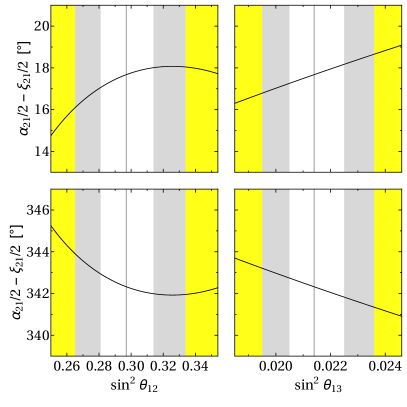
Figure 8: The same as in Fig. 7, but for case A2.

References

- [1] K. Nakamura and S. T. Petcov, in K. A. Olive et al. (Particle Data Group), Chin. Phys. C 38 (2014) 090001.
- [2] S. T. Petcov, Nucl. Phys. B 892 (2015) 400.
- [3] I. Girardi, S. T. Petcov and A. V. Titov, Nucl. Phys. B 894 (2015) 733.
- [4] I. Girardi, S. T. Petcov and A. V. Titov, Eur. Phys. J. C 75 (2015) 345.
- [5] I. Girardi, S. T. Petcov, A. J. Stuart and A. V. Titov, Nucl. Phys. B 902 (2016) 1.
- [6] D. Marzocca, S. T. Petcov, A. Romanino and M. C. Sevilla, JHEP 1305 (2013) 073.
- [7] S. F. King and C. Luhn, Rept. Prog. Phys. 76 (2013) 056201.
- [8] S. F. King et al., New J. Phys. 16 (2014) 045018.
- [9] S. M. Bilenky, J. Hosek and S. T. Petcov, Phys. Lett. B 94 (1980) 495.
- [10] S. M. Bilenky and S. T. Petcov, Rev. Mod. Phys. 59 (1987) 671.
- [11] R.N. Mohapatra et al., Rep. Prog. Phys. 70 (2007) 1757; M. Tanimoto, AIP Conf. Proc. 1666 (2015) 120002.
- [12] P. Minkowski, Phys. Lett. B 67 (1977) 421; T. Yanagida in Proc. of the Workshop on Unified Theory and Baryon Number of the Universe, KEK, Japan, 1979; M. Gell-Mann, P. Ramond and R. Slansky, talk at the Sanibel conference, Feb. 1979, and Print 80-0576, published in Supergravity (North Holland, Amsterdam 1979); S.L.Glashow, Cargese Lectures (1979); R. N. Mohapatra and G. Senjanovic, Phys. Rev. Lett. 44 (1980) 912.
- [13] P. Langacker et al., Nucl. Phys. B 282 (1987) 589.
- [14] S. T. Petcov, Adv. High Energy Phys. 2013 (2013) 852987.
- [15] S.M. Bilenky, S. Pascoli and S.T. Petcov, Phys. Rev. D 64 (2001) 053010.
- [16] W. Rodejohann, Int. J. Mod. Phys. E 20 (2011) 1833; J. D. Vergados, H. Ejiri and F. Simkovic, Rept. Prog. Phys. 75 (2012) 106301.
- [17] S. Pascoli et al., Phys. Lett. B 564 (2003) 241; S. T. Petcov, T. Shindou and Y. Takanishi, Nucl. Phys. B 738 (2006) 219.
- [18] D. N. Dinh, A. Ibarra, E. Molinaro and S. T. Petcov, JHEP 1208 (2012) 125, Erratum: JHEP 1309 (2013) 023.
- [19] S. Pascoli, S. T. Petcov and A. Riotto, Nucl. Phys. B 774 (2007) 1; see also: Phys. Rev. D 75 (2007) 083511.
- [20] M. Fukugita and T. Yanagida, Phys. Lett. B 174 (1986) 45.
- [21] V.A. Kuzmin et al., Phys. Lett. B 155 (1985) 36.
- [22] L. Wolfenstein, Phys. Lett. B 107 (1981) 77; S.M. Bilenky, N.P. Nedelcheva and S.T. Petcov, Nucl. Phys. B 247 (1984) 61; B. Kayser, Phys. Rev. D 30 (1984) 1023.
- [23] E. Molinaro and S. T. Petcov, Eur. Phys. J. C 61 (2009) 93.
- [24] F. Capozzi et al., arXiv:1601.07777.
- [25] F. Capozzi et al., Phys. Rev. D 89 (2014) 093018.
- [26] M. C. Gonzalez-Garcia, M. Maltoni and T. Schwetz, JHEP 1411 (2014) 052, and arXiv:1512.06856.
- [27] P. Adamson et al. [NOvA Collaboration], arXiv:1601.05022.
- [28] P. H. Frampton, S. T. Petcov and W. Rodejohann, Nucl. Phys. B 687 (2004) 31.
- [29] Z. z. Xing, Phys. Lett. B 533 (2002) 85.
- [30] P. F. Harrison, D. H. Perkins and W. G. Scott, Phys. Lett. B 530 (2002) 167; P. F. Harrison and W. G. Scott, Phys. Lett. B 535 (2002) 163; X. G. He and A. Zee, Phys. Lett. B 560 (2003) 87; see also: L. Wolfenstein, Phys. Rev. D 18 (1978) 958.
- [31] S. T. Petcov, Phys. Lett. B 110 (1982) 245.
- [32] F. Vissani, hep-ph/9708483; V. D. Barger, S. Pakvasa, T. J. Weiler and K. Whisnant, Phys. Lett. B 437 (1998) 107; A. J. Baltz, A. S. Goldhaber and M. Goldhaber, Phys. Rev. Lett. 81 (1998) 5730.
- [33] Y. Kajiyama, M. Raidal and A. Strumia, Phys. Rev. D 76 (2007) 117301.
- [34] L. L. Everett and A. J. Stuart, Phys. Rev. D 79 (2009) 085005.
- [35] W. Rodejohann, Phys. Lett. B 671 (2009) 267; A. Adulpravitchai, A. Blum and W. Rodejohann, New J. Phys. 11 (2009) 063026.
- [36] C. H. Albright, A. Dueck and W. Rodejohann, Eur. Phys. J. C 70 (2010) 1099.
- [37] J. E. Kim and M. S. Seo, JHEP 1102 (2011) 097.
- [38] G. Altarelli and F. Feruglio, Rev. Mod. Phys. 82 (2010) 2701.
- [39] F. Feruglio, C. Hagedorn, Y. Lin and L. Merlo, Nucl. Phys. B 775 (2007) 120, Erratum: Nucl. Phys. 836 (2010) 127.
- [40] G. Altarelli, F. Feruglio and L. Merlo, JHEP 0905 (2009) 020.
- [41] F. Bazzocchi, arXiv:1108.2497.
- [42] W. Rodejohann and H. Zhang, Phys. Lett. B 732 (2014) 174.
- [43] R. d. A. Toorop, F. Feruglio and C. Hagedorn, Phys. Lett. B 703 (2011) 447; G. J. Ding, Nucl. Phys. B 862 (2012) 1.
- [44] S. F. King, C. Luhn and A. J. Stuart, Nucl. Phys. B 867 (2013) 203.
- [45] J. Gehrlein, J. P. Oppermann, D. Schäfer and M. Spinrath, Nucl. Phys. B 890 (2014) 539.
- [46] A. Meroni, S. T. Petcov and M. Spinrath, Phys. Rev. D 86 (2012) 113003.
- [47] D. Marzocca, S. T. Petcov, A. Romanino and M. Spinrath, JHEP 1111 (2011) 009.
- [48] S. Antusch, C. Gross, V. Maurer and C. Sluka, Nucl. Phys. B 866 (2013) 255.
- [49] I. Girardi, A. Meroni, S. T. Petcov and M. Spinrath, JHEP 1402 (2014) 050.
- [50] M. C. Chen and K. T. Mahanthappa, Phys. Lett. B 681 (2009) 444; M. C. Chen, J. Huang, K. T. Mahanthappa and A. M. Wijangco, JHEP 1310 (2013) 112.
- [51] P. I. Krastev and S. T. Petcov, Phys. Lett. B 205 (1988) 84.
- [52] G. C. Branco, L. Lavoura and M. N. Rebelo, Phys. Lett. B 180 (1986) 264.
- [53] F. Feruglio, C. Hagedorn and R. Ziegler, JHEP 1307 (2013) 027.
- [54] M. Holthausen, M. Lindner and M. A. Schmidt, JHEP 1304 (2013) 122.
- [55] P. Ballett, S. Pascoli and J. Turner, Phys. Rev. D 92 (2015) no.9, 093008.
- [56] J. Turner, Phys. Rev. D 92 (2015) no.11, 116007.
- [57] J. F. Nieves and P. B. Pal, Phys. Rev. D 36 (1987) 315; Phys. Rev. D 64 (2001) 076005.
- [58] J. A. Aguilar-Saavedra and G. C. Branco, Phys. Rev. D 62 (2000) 096009.
- [59] S. Pascoli and S.T. Petcov, Phys. Lett. B 544 (2002) 239; Phys. Lett. B 580 (2004) 280.
- [60] S. Dell’Oro et al., arXiv:1601.07512.
- [61] S. Pascoli, S.T. Petcov and L. Wolfenstein, Phys. Lett. B 524 (2002) 319; W. Rodejohann, Nucl. Phys. B 597 (2001) 110; S. Pascoli, S.T. Petcov and W. Rodejohann, Phys. Lett. B 549 (2002) 177; S. Pascoli, S.T. Petcov and T. Schwetz, Nucl. Phys. B 734 (2006) 24.
- [62] M. Agostini et al. [GERDA Collaboration], Phys. Rev. Lett. 111 (2013) 12, 122503.
- [63] K. Eitel, Nucl. Phys. Proc. Suppl. 143 (2005) 197.
- [64] S.T. Petcov and C.N. Leung, Phys. Lett. B 125 (1983) 461; S.T. Petcov and S. Toshev, Phys. Lett. B 143 (1984) 175.
- [65] L. L. Everett, T. Garon and A. J. Stuart, JHEP 1504 (2015) 069.
- [66] G. Altarelli and F. Feruglio, Nucl. Phys. B 741 (2006) 215.
- [67] G. J. Ding, S. F. King and A. J. Stuart, JHEP 1312 (2013) 006.
- [68] G. J. Ding, L. L. Everett and A. J. Stuart, Nucl. Phys. B 857 (2012) 219.
- [69] C. C. Li and G. J. Ding, JHEP 1505 (2015) 100.