Nonparametric homogeneity tests and multiple change-point estimation for analyzing large Hi-C data matrices

Abstract.

We propose a novel nonparametric approach for estimating the location of block boundaries (change-points) of non-overlapping blocks in a random symmetric matrix which consists of random variables having their distribution changing from one block to the other. Our method is based on a nonparametric two-sample homogeneity test for matrices that we extend to the more general case of several groups. We first provide some theoretical results for the two associated test statistics and we explain how to derive change-point location estimators. Then, some numerical experiments are given in order to support our claims. Finally, our approach is applied to Hi-C data which are used in molecular biology for better understanding the influence of the chromosomal conformation on the cells functioning.

1. Introduction

Detecting and localizing changes in the distribution of random variables is a major statistical issue that arises in many fields such as the surveillance of industrial processes, see Basseville and Nikiforov (1993), the detection of anomalies in internet traffic data, see Tartakovsky et al. (2006) and Lévy-Leduc and Roueff (2009) or in molecular biology. In the latter field, several change-point detection methods have been designed for dealing with different kinds of data such as CNV (Copy Number Variation), see Picard et al. (2005); Vert and Bleakley (2010), RNAseq data, see Cleynen et al. (2013) and more recently Hi-C data which motivated this work.

The Hi-C technology corresponds to one of the most recent chromosome conformation capture method that has been developed to better understand the influence of the chromosomal conformation on the cells functioning. This technology is based on a deep sequencing approach and provides read pairs corresponding to pairs of genomic loci that physically interacts in the nucleus, see Lieberman-Aiden et al. (2009). The raw measurements provided by Hi-C data are often summarized as a square matrix where each entry at row $i$ and column $j$ stands for the total number of read pairs matching in position $i$ and position $j$, respectively, see Dixon et al. (2012) for further details. Blocks of different intensities arise among this matrix, revealing interacting genomic regions among which some have already been confirmed to host co-regulated genes. The purpose of the statistical analysis is then to provide a fully automated and efficient strategy to determine a decomposition of the matrix in non-overlapping blocks, which gives, as a by-product, a list of non-overlapping interacting chromosomic regions. It has to be noticed that this issue has already been addressed by Lévy-Leduc et al. (2014) in the particular framework where the mean of the observations changes from one diagonal block to the other and is constant everywhere else. In this latter work, the authors use a parametric approach based on the maximization of the likelihood. In the following, we shall address the case where the non-overlapping blocks are not diagonal anymore by using a nonparametric method. Our goal will thus be to design an efficient, nonparametric and fully automated method to find the block boundaries, also called change-points, of non-overlapping blocks in large matrices which can be modeled as matrices of random variables having their distribution changing from one block to the other.

To the best of our knowledge the most recent paper dealing with the nonparametric change-point estimation issue is the one of Matteson and James (2014). Their approach allows them to retrieve change-points within $n$ $K$-dimensional multivariate observations where $K$ is fixed and $n$ may be large. It is based on the use of an empirical divergence measure derived from the divergence measure introduced by Szekely and Rizzo (2005). Note that this methodology cannot be used in our framework since we have to deal with matrices having both their rows and columns that may be large. Another approach based on ranks has also been proposed by Lung-Yut-Fong et al. (2015) in the same framework as Matteson and James (2014). More precisely, the approach proposed by Lung-Yut-Fong et al. (2015) consists in extending the classical Wilcoxon and Kruskal-Wallis statistics (Lehmann and D’Abrera (2006)) to the multivariate case.

In this paper, we propose a nonparametric change-point estimation approach based on nonparametric homogeneity tests. More precisely, we shall generalize the approach of Lung-Yut-Fong et al. (2015) to the case where we have to deal with large matrices instead of fixed multidimensional vectors.

The paper is organized as follows. We first propose in Sections 2.1 and 2.2 nonparametric homogeneity tests for two-samples and several samples, respectively. In Section 2.3, we deduce from these tests a nonparametric procedure for estimating the block boundaries of a matrix of random variables having their distribution changing from one block to the other. These methodologies are then illustrated by some numerical experiments in Section 3. An application to real Hi-C data is also given in Section 4. Finally, the proofs of our theoretical results are given in Section 6.

2. Homogeneity tests and multiple change-point estimation

2.1. Two-sample homogeneity test

2.1.1. Statistical framework

Let $\textbf{X}=(X_{i,j})_{1\leq i,j\leq n}$ be a symmetric matrix such that the $X_{i,j}$’s are independent random variables when $i\geq j$. Observe that X can be rewritten as follows: $\textbf{X}=(\textbf{X}^{(1)},\ldots,\textbf{X}^{(n)})$, where $\textbf{X}^{(j)}=(X_{1,j},\ldots,X_{n,j})^{\prime}$ denotes the $j$th column of X.

Let $n_{1}$ be a given integer in $\{1,\dots,n\}$. The goal of this section is to propose a statistic to test the null hypothesis $(H_{0})$: “$(\textbf{X}^{(1)},\ldots,\textbf{X}^{(n_{1})})$ and $(\textbf{X}^{(n_{1}+1)},\ldots,\textbf{X}^{(n)})$ are identically distributed random vectors” against the alternative hypothesis $(H_{1})$: “$(\textbf{X}^{(1)},\ldots,\textbf{X}^{(n_{1})})$ has the distribution $\mathbb{P}_{1}$ and $(\textbf{X}^{(n_{1}+1)},\ldots,\textbf{X}^{(n)})$ has the distribution $\mathbb{P}_{2}$, where $\mathbb{P}_{1}\neq\mathbb{P}_{2}$”. Note that the hypotheses $(H_{0})$ and $(H_{1})$ can be reformulated as follows. The null hypothesis $(H_{0})$ means that for all $i\in\{1,\ldots,n\}$, $X_{i,1},\ldots,X_{i,n}$ are independent and identically distributed (i.i.d) random variables and the alternative hypothesis $(H_{1})$ means that there exists $i\in\{1,\ldots,n\}$ such that $X_{i,1},\ldots,X_{i,n_{1}}$ have the distribution $\mathbb{P}^{i}_{1}$ and $X_{i,n_{1}+1},\ldots,X_{i,n}$ have the distribution $\mathbb{P}^{i}_{2}$, with $\mathbb{P}^{i}_{1}\neq\mathbb{P}^{i}_{2}$.

For deciding whether $(H_{0})$ has to be rejected or not, we propose to use a test statistic inspired by the one designed by Lung-Yut-Fong et al. (2015) which extends the well-known Wilcoxon-Mann-Whitney rank-based test to deal with multivariate data. Our statistical test can thus be seen as a way to decide whether $n_{1}$ can be considered as a potential change in the distribution of the $X_{i,j}$’s or not. More precisely, the test statistic that we propose for assessing the presence of the potential change $n_{1}$ is defined by

$$S_{n}(n_{1})=\sum_{i=1}^{n}U_{n,i}^{2}(n_{1}),$$ (1)

where

$$U_{n,i}(n_{1})=\frac{1}{\sqrt{nn_{1}(n-n_{1})}}\sum_{j_{0}=1}^{n_{1}}\sum_{j_{1}=n_{1}+1}^{n}h(X_{i,j_{0}},X_{i,j_{1}}),$$

with $h(x,y)=\mathbbm{1}_{\{x\leq y\}}-\mathbbm{1}_{\{y\leq x\}}$.

The great difference between our framework and the one considered by Lung-Yut-Fong et al. (2015) is that, in their framework, the vectors $\textbf{X}^{(j)}$ are $K$-dimensional with $K$ fixed whereas, in our framework, the vectors are $n$-dimensional where $n$ may be large.

Note that the statistic $U_{n,i}$ can also be written by using the rank of $X_{i,j}$ among $\left(X_{i,1},\ldots,X_{i,n}\right)$. Indeed,

$$U_{n,i}(n_{1})=\frac{2}{\sqrt{nn_{1}(n-n_{1})}}\sum_{j_{0}=1}^{n_{1}}\left(\frac{n+1}{2}-R_{j_{0}}^{(i)}\right)=\frac{2}{\sqrt{nn_{1}(n-n_{1})}}\sum_{j_{1}=n_{1}+1}^{n}\left(R_{j_{1}}^{(i)}-\frac{n+1}{2}\right),$$ (2)

where

$$R_{j}^{(i)}=\sum_{k=1}^{n}\mathbbm{1}_{\{X_{i,k}\leq X_{i,j}\}}$$ (3)

is the rank of $X_{i,j}$ among $\left(X_{i,1},\ldots,X_{i,n}\right)$. This alternative form of $U_{n,i}$ will be used in Section 2.2 in order to extend the two-sample homogeneity test to deal with the multiple sample case.

2.1.2. Theoretical results

If the cumulative distribution function of the $X_{i,j}$’s is assumed to be continuous then the following theorem establishes that the test statistic $S_{n}(n_{1})$ is properly normalized, namely $S_{n}(n_{1})$ is bounded in probability as $n$ tends to infinity.

Theorem 1.

Let $\textbf{X}=(X_{i,j})_{1\leq i,j\leq n}$ be a symmetric matrix of random variables $X_{i,j}$ such that the $X_{i,j}$’s are i.i.d. when $i\geq j$. Assume that the cumulative distribution function of the $X_{i,j}$’s is continuous and that there exists $\tau_{1}\in(0,1)$ such that $n_{1}/n\rightarrow\tau_{1}$ as $n\to\infty$. Then,

$$T_{n}(n_{1}):=n^{-1/2}\big{(}S_{n}(n_{1})-\mathbb{E}(S_{n}(n_{1})\big{)}=O_{P}(1)\mbox{ as }n\to\infty,$$

where

$$\mathbb{E}(S_{n}(n_{1}))=\frac{n+1}{3}.$$

The proof of Theorem 1 is given in Section 6.1.

Observe that the assumptions under which Theorem 1 is established correspond to the null hypothesis $(H_{0})$ described in Section 2.1.1. Hence, we shall reject this null hypothesis when

$$T_{n}(n_{1})>s,$$ (4)

where $s$ is a threshold. A way of computing this threshold in practical situations will be given in Section 3.1.1.

2.2. Multiple-sample homogeneity test

The goal of this section is to extend the two-sample homogeneity test of the previous section to deal with the multiple sample case.

2.2.1. Statistical framework

Let us assume that $\textbf{X}=(X_{i,j})_{1\leq i,j\leq n}$ is still a symmetric matrix such that the $X_{i,j}$’s are independent random variables when $i\geq j$. Let $0=n_{0}<n_{1}<\ldots<n_{L}<n_{L+1}=n$ be $L$ integers given in $\{1,\dots,n-1\}$. We propose in this section a statistic to test the null hypothesis: “$(\textbf{X}^{(1)},\ldots,\textbf{X}^{(n_{1})})$, $(\textbf{X}^{(n_{1}+1)},\ldots,\textbf{X}^{(n_{2})})$, …,$(\textbf{X}^{(n_{L}+1)},\ldots,\textbf{X}^{(n)})$ have the same distribution” against the alternative hypothesis: “there exists $\ell\in\{1,\ldots,L\}$ such that $(\textbf{X}^{(n_{\ell-1}+1)},\ldots,\textbf{X}^{(n_{\ell})})$ has the distribution $\mathbb{P}_{\ell}$ and $(\textbf{X}^{(n_{\ell}+1)},\ldots,\textbf{X}^{(n_{\ell+1})})$ has the distribution $\mathbb{P}_{\ell+1}$, where $\mathbb{P}_{\ell}\neq\mathbb{P}_{\ell+1}$”.

The homogeneity test presented in the previous section for two groups can be extended in order to deal with $L+1$ groups instead of two by using the following statistic:

$$S_{n}\left(n_{1},\ldots,n_{L}\right)=\frac{4}{n^{2}}\sum_{\ell=0}^{L}\left(n_{\ell+1}-n_{\ell}\right)\sum_{i=1}^{n}\left(\overline{R}_{\ell}^{(i)}-\frac{n+1}{2}\right)^{2},$$ (5)

with

$$\overline{R}_{\ell}^{(i)} = \frac{1}{n_{\ell+1}-n_{\ell}}\sum_{j=n_{\ell}+1}^{n_{\ell+1}}R_{j}^{(i)},$$ (6)

where the rank $R_{j}^{(i)}$ of $X_{i,j}$ is defined by (3) and $\overline{R}_{\ell}^{(i)}$ is its mean in the group $\ell$.

Let us observe that (5) can be seen as a natural extension of the classical Kruskal-Wallis statistic for univariate observations to the multivariate case, see (van der Vaart, 1998, p. 181).

Remark 1.

Note that when $L=1$, $S_{n}(n_{1})$ defined in (5) boils down to $S_{n}(n_{1})$ defined in (1) since

$$\frac{4}{n^{2}}\left[n_{1}\sum_{i=1}^{n}\left(\frac{1}{n_{1}}\sum_{j=1}^{n_{1}}R_{j}^{(i)}-\frac{n+1}{2}\right)^{2}+(n-n_{1})\sum_{i=1}^{n}\left(\frac{1}{n-n_{1}}\sum_{j=n_{1}+1}^{n}R_{j}^{(i)}-\frac{n+1}{2}\right)^{2}\right]$$

$$=\frac{4}{n^{2}n_{1}}\sum_{i=1}^{n}\left\{\sum_{j=1}^{n_{1}}\left(R_{j}^{(i)}-\frac{n+1}{2}\right)\right\}^{2}+\frac{4}{n^{2}(n-n_{1})}\sum_{i=1}^{n}\left\{\sum_{j=n_{1}+1}^{n}\left(R_{j}^{(i)}-\frac{n+1}{2}\right)\right\}^{2}$$

$$=\frac{1}{n}\left[\sum_{i=1}^{n}n_{1}\left\{\frac{1}{\sqrt{nn_{1}(n-n_{1})}}\sum_{j=1}^{n_{1}}\left(R_{j}^{(i)}-\frac{n+1}{2}\right)\right\}^{2}\right.$$

$$\left.+\sum_{i=1}^{n}(n-n_{1})\left\{\frac{1}{\sqrt{nn_{1}(n-n_{1})}}\sum_{j=n_{1}+1}^{n}\left(R_{j}^{(i)}-\frac{n+1}{2}\right)\right\}^{2}\right]=\sum_{i=1}^{n}U_{n,i}^{2}(n_{1}),$$

by using (2), which corresponds to (1).

2.2.2. Theoretical results

If the cumulative distribution function of the $X_{i,j}$’s is assumed to be continuous then the following theorem establishes that the test statistic $S_{n}\left(n_{1},\ldots,n_{L}\right)$ is properly normalized, namely $S_{n}\left(n_{1},\ldots,n_{L}\right)$ is bounded in probability as $n$ tends to infinity.

Theorem 2.

Let $\textbf{X}=(X_{i,j})_{1\leq i,j\leq n}$ be a symmetric matrix of random variables $X_{i,j}$ such that the $X_{i,j}$’s are i.i.d when $i\geq j$. Assume that the cumulative distribution function of the $X_{i,j}$’s is continuous and that there exist $0<\tau_{1}<\tau_{2}<\ldots<\tau_{L}<1$ such that for all $\ell\in\{1,\ldots,L\}$, $n_{\ell}/n\rightarrow\tau_{\ell}$ as $n\to\infty$. Then,

$$n^{-1/2}\big{(}S_{n}\left(n_{1},\ldots,n_{L}\right)-\mathbb{E}\left[S_{n}\left(n_{1},\ldots,n_{L}\right)\right]\big{)}=O_{P}(1)\mbox{ as }n\to\infty,$$

with

$$\mathbb{E}\left[S_{n}\left(n_{1},\ldots,n_{L}\right)\right]=\frac{L(n+1)}{3}.$$

The proof of Theorem 2 is given in Section 6.2

Note that the $n_{\ell}$’s can be seen as the boundaries of groups of random variables having different distributions. We shall explain in the next section how to derive from this theorem a methodology for estimating the $n_{\ell}$’s when they are assumed to be unknown.

2.3. Multiple change-point estimation

We propose in this section to use the test statistic (5) defined in Section 2.2 to derive the location of the block boundaries $n_{1}<n_{2}<\cdots<n_{L}$. More precisely, we propose to estimate $(n_{1},n_{2},\cdots,n_{L})$ as follows:

$$(\widehat{n}_{1},\cdots,\widehat{n}_{L}):=\textrm{Argmax}_{0<n_{1}<\ldots<n_{L}<n}\;S_{n}(n_{1},\ldots,n_{L}),$$ (7)

where $S_{n}(n_{1},\ldots,n_{L})$ is defined in (5).

In practice, directly maximizing (7) is computationally prohibitive as it corresponds to a task which complexity exponentially grows with $L$. However, thanks to the additive structure of (5), it is possible to use a dynamic programming strategy as we shall explain hereafter. We refer here to the classical dynamic programming approach described in Kay (1993) which can be traced back to the note of Bellman (1961).

Let us introduce the following notations

$$\Delta(n_{\ell}+1:n_{\ell+1})=(n_{\ell+1}-n_{\ell})\sum_{i=1}^{n}\left(\overline{R}_{\ell}^{(i)}-\frac{n+1}{2}\right)^{2},$$

where $\overline{R}_{\ell}^{(i)}$ is defined by (6) and

$$I_{L}(p)=\max_{1<n_{1}<\dots<n_{L}<n_{L+1}=p}\sum_{\ell=0}^{L}\Delta(n_{\ell}+1:n_{\ell+1}),$$ (8)

for $L\in\{0,1,\dots,L_{\textrm{max}}\}$ and $p\in\{2,\ldots,n\}$, where $L_{\textrm{max}}$ is assumed to be a known upper bound for the number of block boundaries. Observe that $I_{L}(p)$ satisfies the following recursive formula:

$$I_{L}(p)=\max_{n_{L}}\left\{I_{L-1}(n_{L})+\Delta(n_{L}+1:p)\right\}\;,$$ (9)

which is proved in Section 6.3. Thus, for solving the optimization problem (7), we proceed as follows. We start by computing the $\Delta(i:j)$ for all $(i,j)$ such that $1\leq i<j\leq n$. All the $I_{0}(p)$ are thus available for $p=2,\dots,n$. Then $I_{1}(p)$ is computed by using the recursion (9) and so on. Hence the complexity of our algorithm is $O(n^{3})$.

Figure 1 displays the computational times in seconds associated with our multiple change-point estimation strategy based on the dynamic programming algorithm. We observe from this figure the polynomial computational time of our procedure. For instance, it takes 15 minutes to our algorithm for processing a $500\times 500$ matrix.

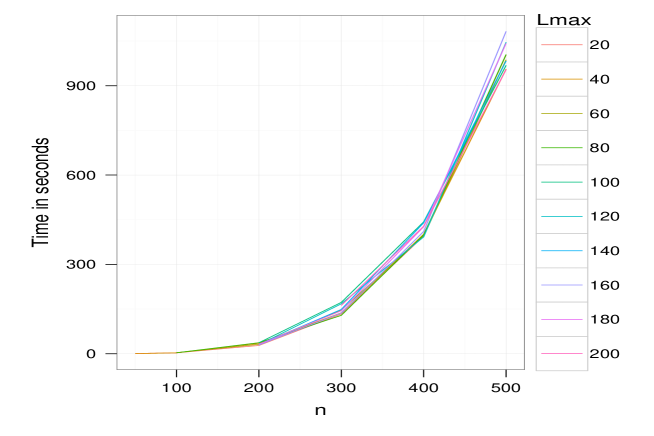
Figure 1. Computational times in seconds for the dynamic programming algorithm described in Section 2.3 as a function of $n$ for different values of $L_{\textrm{max}}$.

3. Numerical experiments

3.1. Statistical performance of the two-sample homogeneity test

3.1.1. Practical calibration of the rejection region

We propose hereafter a procedure for calibrating the threshold $s$ of the rejection region $T_{n}(n_{1})>s$ defined in (4). For ensuring that the two-sample homogeneity test is of level $\alpha$, an estimation of the $(1-\alpha)$ quantile of $T_{n}(n_{1})$ has to be provided. In the sequel, such an estimation is given in the case where $\alpha=0.05$.

We generated $10^{4}$ $n\times n$ symmetric matrices $\boldsymbol{X}=(X_{i,j})$ with $n\in\{50,100,500,1000\}$. More precisely, the $(X_{i,j})_{i\geq j}$’s are independent random variables distributed as a zero mean standard Gaussian distribution ($\mathcal{N}(0,1)$), a Cauchy distribution with 0 and 1 location and scale parameters ($\mathcal{C}au(0,1)$), respectively or an Exponential distribution of parameter 2 ($\mathcal{E}xp(2)$). We shall consider two values for $n_{1}$: $n_{1}=\lfloor 0.1n\rfloor$ and $n_{1}=\lfloor 0.5n\rfloor$, where $\lfloor x\rfloor$ denotes the integer part of $x$.

The empirical $0.95$ quantiles of $T_{n}(n_{1})$ are given in Table 1. We observe from this table that the empirical $0.95$ quantiles do not seem to be sensitive neither to the values of $n_{1}$ and $n$ nor to the distribution of the observations since they slightly vary around 0.8.

	$n_{1}=\lfloor 0.1n\rfloor$			$n_{1}=\lfloor 0.5n\rfloor$
	$\mathcal{N}(0,1)$	$\mathcal{C}au(0,1)$	$\mathcal{E}xp(2)$	$\mathcal{N}(0,1)$	$\mathcal{C}au(0,1)$	$\mathcal{E}xp(2)$
$n=50$	0.83	0.83	0.82	0.78	0.79	0.76
$n=100$	0.81	0.8	0.82	0.78	0.8	0.78
$n=500$	0.78	0.8	0.81	0.8	0.78	0.77
$n=1000$	0.79	0.78	0.79	0.78	0.77	0.79

Table 1. Estimation of the empirical $0.95$ quantiles of $T_{n}(n_{1})$.

3.1.2. Power of the test statistic

In this section, we study the power of the two-sample homogeneity test defined in Section 2.1.1. We generated $10^{4}$ $n\times n$ symmetric matrices $\boldsymbol{X}=(X_{i,j})$ split into four blocks defined as follows and $n\in\{50,100,500,1000\}$. Let

$$\mathcal{I}_{1}=\{(i,j):1\leq j\leq i\leq n_{1}\},\;\;\mathcal{I}_{2}=\{(i,j):1\leq j\leq n_{1},\;n_{1}+1\leq i\leq n\},$$

and

$$\mathcal{I}_{3}=\{(i,j):n_{1}+1\leq j\leq i\leq n\}.$$

In the sequel, we assume that $(X_{i,j})_{(i,j)\in\mathcal{I}_{1}}\stackrel{{\scriptstyle iid}}{{\sim}}\mathcal{L}_{1}$, $(X_{i,j})_{(i,j)\in\mathcal{I}_{2}}\stackrel{{\scriptstyle iid}}{{\sim}}\mathcal{L}_{2}$ and $(X_{i,j})_{(i,j)\in\mathcal{I}_{3}}\stackrel{{\scriptstyle iid}}{{\sim}}\mathcal{L}_{3}$ and we take the following values for $n_{1}$: $n_{1}=\lfloor 0.1n\rfloor$ and $n_{1}=\lfloor 0.5n\rfloor$.

Figure 2 displays the power curves of the two-sample homogeneity test defined in Section 2.1.1 in the case where $\mathcal{L}_{1}=\mathcal{L}_{3}=\mathcal{N}(0,1)$ and $\mathcal{L}_{2}=\mathcal{N}(\mu,1)$ where $\mu$ belongs to the set $\{0,0.01,0.02,\dots,0.99,1\}$.

We can see from this figure that for large values of $n$ our testing procedure appears to be powerful whatever the value of $\mu$. For small values of $n$, we observe that our testing procedure is all the more powerful that $\mu$ is large.

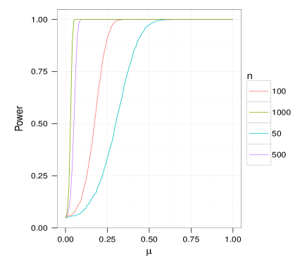
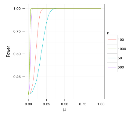
Figure 2. Power curves for the two-sample homogeneity test as a function of $\mu$ for different values of $n$, $n_{1}=\lfloor 0.1n\rfloor$ (left) and $n_{1}=\lfloor 0.5n\rfloor$ (right).

3.2. Statistical performance of the multiple change-point estimation procedure

In this section, we study the statistical performance of the multiple change-point estimation procedure described in Section 2.3. This method is implemented in the R package MuChPoint, which will be available on the Comprehensive R Archive Network (CRAN).

We generated 10000 $n\times n$ symmetric matrices $\textbf{X}=(X_{i,j})$ where $n\in\{50,100,200,300,400\}$ with different block configurations and $L=10$ block boundaries (change-points).

We shall first consider the Block Diagonal configuration. In this case, the matrix consists of diagonal blocks of size $n/10$. Within each of these diagonal blocks, the $X_{i,j}$’s such that $i\geq j$ are independent and have the distribution $\mathcal{L}_{1}$. The $X_{i,j}$’s lying in the extra-diagonal part of the lower triangular part of X are independent and have the distribution $\mathcal{L}_{2}$, which is assumed to be different from $\mathcal{L}_{1}$. The upper triangular part of X is then derived by symmetry.

We shall also consider the Chessboard configuration. In this case, the matrix consists of non overlapping blocks of size $n/10$. The $X_{i,j}$’s belonging to two blocks sharing a boundary have different distributions. This configuration implies that only two distributions $\mathcal{L}_{1}$ and $\mathcal{L}_{2}$ are at stake. The distribution of the upper left block is denoted by $\mathcal{L}_{1}$ in the sequel.

For these two configurations, we shall consider for $\mathcal{L}_{1}$ a $\mathcal{N}(1,\sigma^{2})$, a $\mathcal{E}xp(2)$ or a $\mathcal{C}au(1,a)$ distribution where $\sigma$ and $a$ are in $\{1,2,5\}$. The $\mathcal{L}_{2}$ distributions associated with each of them are $\mathcal{N}(0,\sigma^{2})$, $\mathcal{E}xp(\lambda)$ and $\mathcal{C}au(0,a)$ where $\lambda\in\{1,0.5,4\}$. We display in Figure 3 some examples of the Block Diagonal and Chessboard configurations for the Gaussian, Exponential and Cauchy distributions. In these plots, large values are displayed in red and small values in blue.

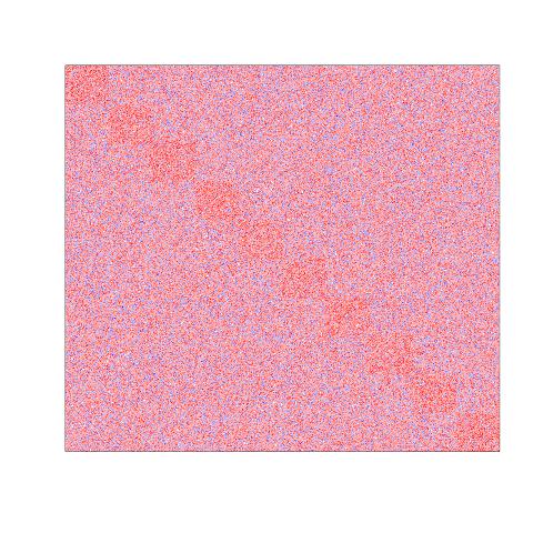
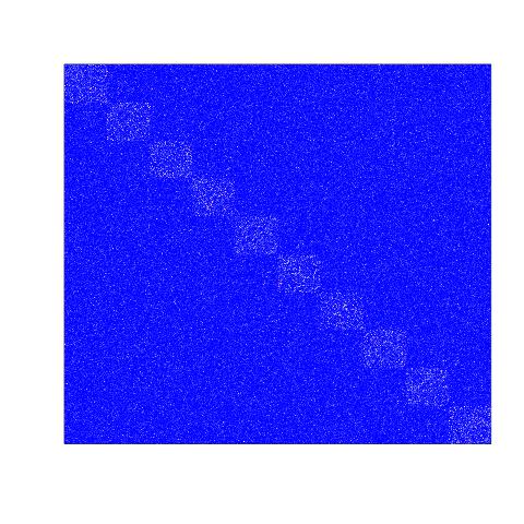
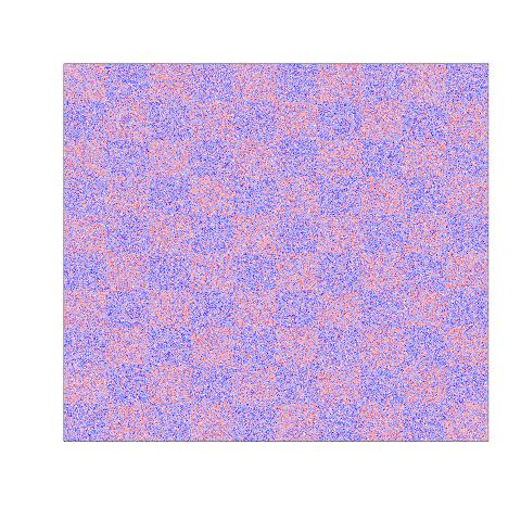
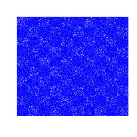
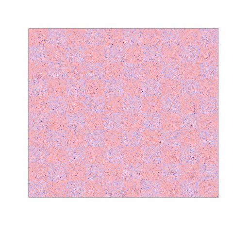
Figure 3. Examples of $400\times 400$ matrices X. Top: Block Diagonal configuration. Bottom: Chessboard configuration. Left: $\mathcal{L}_{1}=\mathcal{N}(1,4)$, $\mathcal{L}_{2}=\mathcal{N}(0,4)$, middle: $\mathcal{L}_{1}=\mathcal{E}xp(2)$, $\mathcal{L}_{2}=\mathcal{E}xp(1)$ and right: $\mathcal{L}_{1}=\mathcal{C}au(1,1)$, $\mathcal{L}_{2}=\mathcal{C}au(0,1)$.

In the Gaussian Chessboard configuration, Figure 4 displays the frequency of the number of times where each position in $\{1,\dots,n-1\}$ has been estimated as a change-point. We can see from this figure that the true change-point positions are in general properly retrieved by our approach even in cases where the change-points are not easy to detect with the naked eye. However, we observe that in the cases where $\sigma$ increases, some spurious change-points appear close to the true change-point positions.

$\sigma=1$	$\sigma=2$	$\sigma=5$

Figure 4. Barplots associated with the multiple change-point estimation procedure for $n=100$ (top), $n=400$ (bottom), $\mathcal{L}_{1}=\mathcal{N}(1,\sigma^{2})$ and $\mathcal{L}_{2}=\mathcal{N}(0,\sigma^{2})$ for different values of $\sigma$. The true positions of the change-points are located at the multiples of $n/10$.

We also compared our multiple change-point estimation strategy (MuChPoint) to the one devised by Matteson and James (2014) (ecp), which is, to the best of our knowledge, the most recent approach proposed for solving this issue. The results are gathered in Figures 5 and 6 which display the boxplots of the distance $D$, defined in (10), between the change-points provided by these procedures in the Block Diagonal and Chessboard configurations for the Gaussian, Exponential and Cauchy distributions. These boxplots are obtained from 100 replications of $n\times n$ symmetric matrices where $n\in\{50,100,200,300,400\}$. More precisely, the distance $D$ is defined as follows

$$D(\widehat{\textbf{t}},\textbf{t}^{\star})=\frac{1}{n}\sqrt{\sum_{k=1}^{K^{\star}}(\widehat{t}_{k}-t_{k}^{\star})^{2}},$$ (10)

where $\textbf{t}^{\star}=(t_{1}^{\star},\dots,t_{K^{\star}}^{\star})$ denotes the vector of the true $K^{\star}$ change-point positions and $\widehat{\textbf{t}}=(\widehat{t}_{1},\dots,\widehat{t}_{K^{\star}})$ its estimation either obtained by MuChPoint or ecp. Note that, it actually corresponds to the usual $\ell_{2}$-norm of the vector $\boldsymbol{\tau}^{\star}-\widehat{\boldsymbol{\tau}}$ where $\boldsymbol{\tau}^{\star}=(\tau_{1}^{\star},\dots,\tau_{K^{\star}}^{\star})$, $\widehat{\boldsymbol{\tau}}=(\widehat{\tau}_{1},\dots,\widehat{\tau}_{K^{\star}})$ with $t_{k}^{\star}=\lfloor n\tau_{k}^{\star}\rfloor$ and $\widehat{t}_{k}=\lfloor n\widehat{\tau}_{k}\rfloor$. In order to benchmark these methodologies, we provide to both of them the true value $K^{\star}$ of the number of change-points, which is here equal to 10.

$\sigma=1$	$a=1$	$\lambda=1/2$
$\sigma=2$	$a=2$	$\lambda=1$
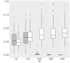
$\sigma=5$	$a=5$	$\lambda=4$

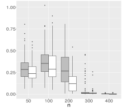
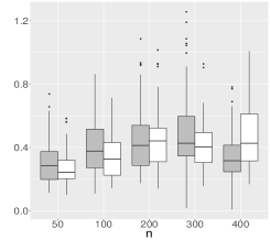
Figure 5. Boxplots of the distances $D$ for MuChPoint and ecp in the Chessboard configuration. Left: $\mathcal{L}_{1}=\mathcal{N}(1,\sigma^{2})$, $\mathcal{L}_{2}=\mathcal{N}(0,\sigma^{2})$, middle: $\mathcal{L}_{1}=\mathcal{C}au(1,a)$, $\mathcal{L}_{2}=\mathcal{C}au(0,a)$ and right: $\mathcal{L}_{1}=\mathcal{E}xp(2)$, $\mathcal{L}_{2}=\mathcal{E}xp(\lambda)$ for different values of $\sigma$, $\lambda$ and $a$. The boxplots associated with MuChPoint are displayed in gray and the ones of ecp in white.

$\sigma=1$	$a=1$	$\lambda=1/2$
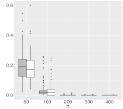
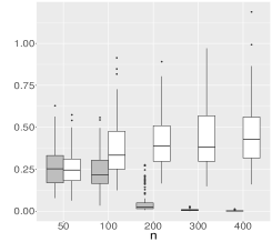
$\sigma=2$	$a=2$	$\lambda=1$
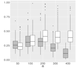
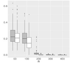
$\sigma=5$	$a=5$	$\lambda=4$

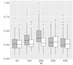
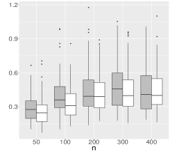
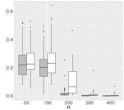
Figure 6. Boxplots of the distances $D$ for MuChPoint and ecp in the Block Diagonal configuration. Left: $\mathcal{L}_{1}=\mathcal{N}(1,\sigma^{2})$, $\mathcal{L}_{2}=\mathcal{N}(0,\sigma^{2})$, middle: $\mathcal{L}_{1}=\mathcal{C}au(1,a)$, $\mathcal{L}_{2}=\mathcal{C}au(0,a)$ and right: $\mathcal{L}_{1}=\mathcal{E}xp(2)$, $\mathcal{L}_{2}=\mathcal{E}xp(\lambda)$ for different values of $\sigma$, $\lambda$ and $a$. The boxplots associated with MuChPoint are displayed in gray and the ones of ecp in white.

We observe from Figures 5 and 6 that both approaches have similar statistical performance. However, MuchPoint performs better than ecp in the Cauchy case. In the Gaussian framework, the performance of ecp are a little bit better for small $n$ and large $\sigma$.

4. Application to real data

In this section, we apply our methodology to publicly available Hi-C data (http://chromosome.sdsc.edu/mouse/hi-c/download.html) already studied by Dixon et al. (2012). This technology provides read pairs corresponding to pairs of genomic loci that physically interacts in the nucleus, see Lieberman-Aiden et al. (2009) for further details. The raw measurements provided by Hi-C data is therefore a list of pairs of locations along the chromosome, at the nucleotide resolution. These measurements are often summarized by a symmetric matrix $\boldsymbol{X}$ where each entry $X_{i,j}$ corresponds the total number of read pairs matching in position $i$ and position $j$, respectively. Positions refer here to a sequence of non-overlapping windows of equal sizes covering the genome. The number of windows may vary from one study to another: Lieberman-Aiden et al. (2009) considered a Mb resolution, whereas Dixon et al. (2012) went deeper and used windows of 40kb (called hereafter the resolution).

In the sequel, we analyze the interaction matrices of Chromosome 19 of the mouse cortex at a resolution 40 kb and we compare the location of the estimated change-points found by our approach with those obtained by Dixon et al. (2012) on the same data since no ground truth is available. In this case, the matrix that has to be processed is a $n\times n$ symmetric matrix where $n=1534$.

We display in Figure 7 the estimated matrix $\widehat{\textbf{X}}$ obtained by using our strategy for various numbers of estimated change-points. This estimated matrix is a block-wise constant matrix for which the block boundaries are estimated by using MuChPoint and the values within each block correspond to the empirical mean of the observations lying in it. We can see from this figure that both the diagonal and the extra diagonal blocks are properly retrieved even when the number of estimated change-points is not that large.

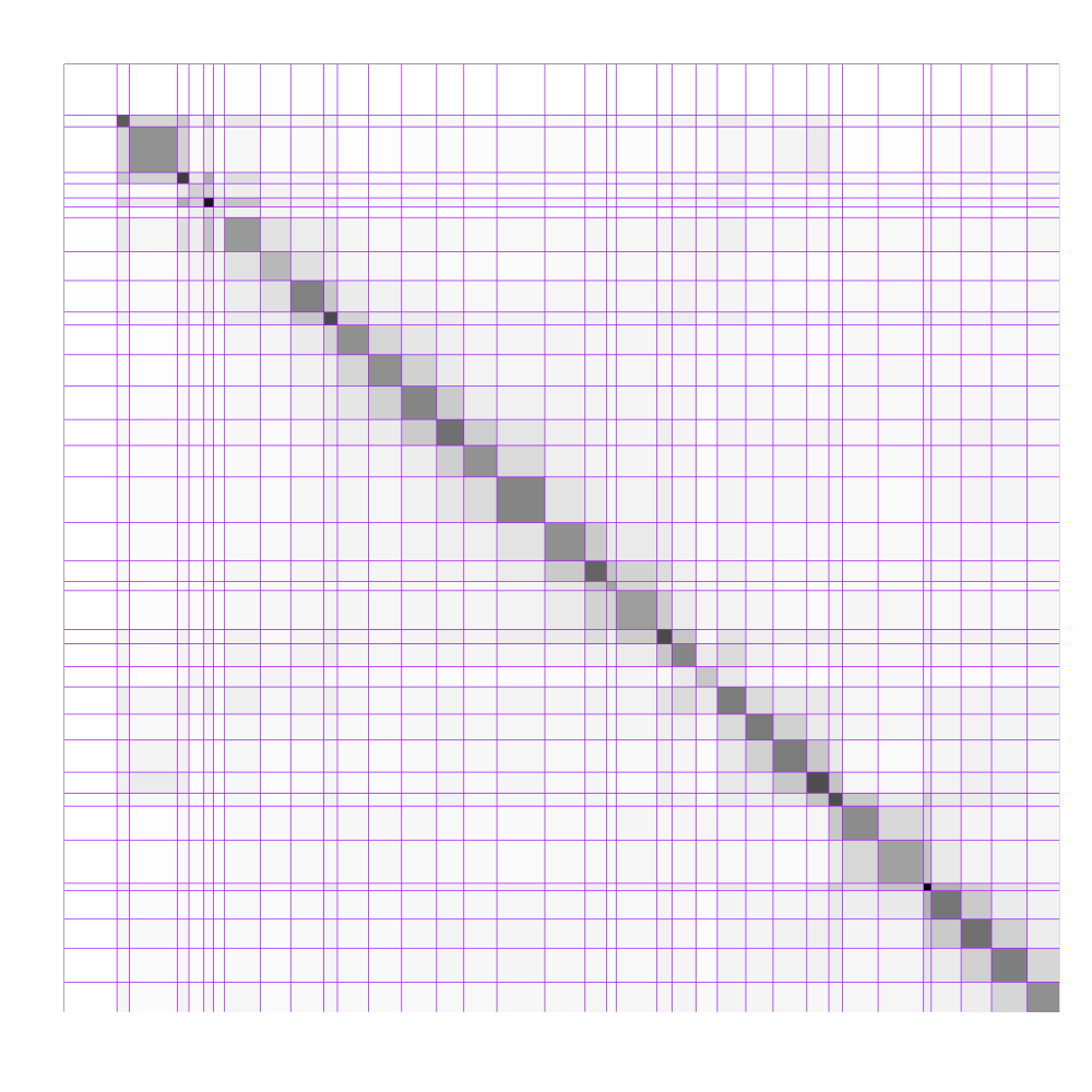
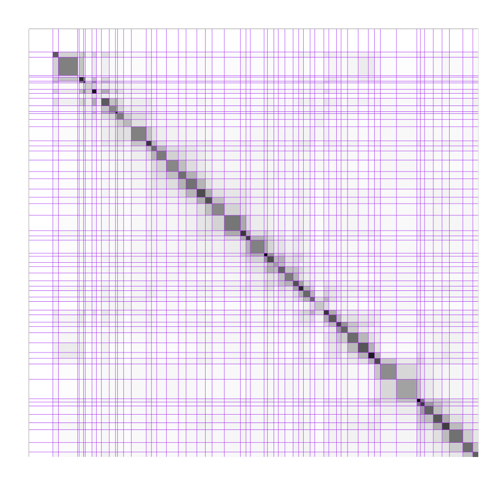
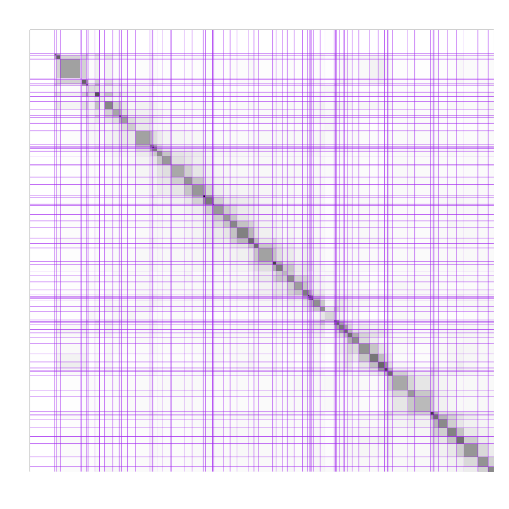
Figure 7. Estimated matrices $\widehat{\textbf{X}}$ for different number of estimated change-points: 35 (left), 55 (middle) and 75 (right).

In order to further compare our approach with the one proposed by Dixon et al. (2012), we computed the two parts of the Hausdorff distance which is defined by

$$d\left(\widehat{\boldsymbol{t}}_{B},\widehat{\boldsymbol{t}}\right)=\max\left(d_{1}\left(\widehat{\boldsymbol{t}}_{B},\widehat{\boldsymbol{t}}\right),d_{2}\left(\widehat{\boldsymbol{t}}_{B},\widehat{\boldsymbol{t}}\right)\right)\;,$$ (11)

where $\widehat{\boldsymbol{t}}$ and $\widehat{\boldsymbol{t}}_{B}$ are the change-points found by our approach and Dixon et al. (2012), respectively. In (11),

$$d_{1}\left(\mathbf{a},\mathbf{b}\right) = \sup_{b\in\mathbf{b}}\inf_{a\in\mathbf{a}}\left|a-b\right|,$$

$$d_{2}\left(\mathbf{a},\mathbf{b}\right) = d_{1}\left(\mathbf{b},\mathbf{a}\right).$$

More precisely, Figure 8 displays the boxplots of the $d_{1}$ and $d_{2}$ parts of the Hausdorff distance without taking the supremum in white and gray for different values of the estimated number of change-points, respectively.

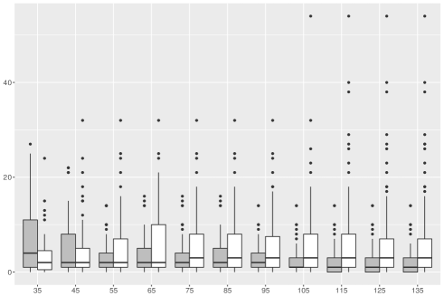
Figure 8. Boxplots for the infimum parts of the Hausdorff distances $d_{1}$ (white) and $d_{2}$ (gray) between the change-points found by Dixon et al. (2012) and our approach for different values of the estimated number of change-points.

We can see from this figure that some differences exist between the two approaches. However, when the number of estimated change-points considered in our methodology is on a par with the one of Dixon et al. (2012), the position of the block boundaries are very close as displayed in Figure 9.

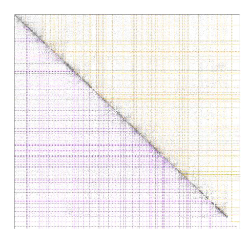
Figure 9. Topological domains detected by Dixon et al. (2012) (upper triangular part of the matrix) and by our method (lower triangular part of the matrix).

5. Conclusion

In this paper, we designed a novel nonparametric and fully automated method for retrieving the block boundaries of non-overlapping blocks in large matrices modeled as symmetric matrices of random variables having their distribution changing from one block to the other. Our approach is implemented in the R package MuChPoint which will be available from the Comprehensive R Archive Network (CRAN). In the course of this study, we have shown that our method, inspired by a generalization of nonparametric multiple sample tests to multivariate data, has two main features which make it very attractive. Firstly, it is a nonparametric approach which showed very good statistical performances from a practical point of view. Secondly, its low computational burden makes its use possible on large Hi-C data matrices.

6. Proofs

In this section, we prove Theorems 1, 2 and Equation (9). The proofs of Theorems 1 and 2 given below use technical lemmas established in Section 7.

6.1. Proof of Theorem 1

For proving Theorem 1, we first compute the expectation of $S_{n}(n_{1})$.

$$\mathbb{E}\left[S_{n}(n_{1})\right] =\sum_{i=1}^{n}\mathbb{E}\left[U_{n,i}^{2}(n_{1})\right]$$

$$=\frac{1}{nn_{1}(n-n_{1})}\sum_{i=1}^{n}\mathbb{E}\left[\left(\sum_{j_{0}=1}^{n_{1}}\sum_{j_{1}=n_{1}+1}^{n}h(X_{i,j_{0}},X_{i,j_{1}})\right)^{2}\right]$$

$$=\frac{1}{nn_{1}(n-n_{1})}\sum_{i=1}^{n}\sum_{1\leq j_{0},k_{0}\leq n_{1}}\sum_{n_{1}+1\leq j_{1},k_{1}\leq n}\mathbb{E}\left[h(X_{i,j_{0}},X_{i,j_{1}})h(X_{i,k_{0}},X_{i,k_{1}})\right]$$

$$=\frac{1}{nn_{1}(n-n_{1})}\sum_{i=1}^{n}\left\{\sum_{j_{0}=1}^{n_{1}}\sum_{j_{1}=n_{1}+1}^{n}\mathbb{E}\left[h^{2}(X_{i,j_{0}},X_{i,j_{1}})\right]\right.$$

$$\quad+\sum_{j_{0}=1}^{n_{1}}\sum_{n_{1}+1\leq j_{1}\neq k_{1}\leq n}\mathbb{E}\left[h(X_{i,j_{0}},X_{i,j_{1}})h(X_{i,j_{0}},X_{i,k_{1}})\right]$$

$$\quad+\sum_{1\leq j_{0}\neq k_{0}\leq n_{1}}\sum_{j_{1}=n_{1}+1}^{n}\mathbb{E}\left[h(X_{i,j_{0}},X_{i,j_{1}})h(X_{i,k_{0}},X_{i,j_{1}})\right]$$

$$\quad\left.+\sum_{1\leq j_{0}\neq k_{0}\leq n_{1}}\sum_{n_{1}+1\leq j_{1}\neq k_{1}\leq n}\mathbb{E}\left[h(X_{i,j_{0}},X_{i,j_{1}})h(X_{i,k_{0}},X_{i,k_{1}})\right]\right\}.$$

By using Lemma 1, we get that

$$\mathbb{E}\left[S_{n}(n_{1})\right] =\frac{1}{nn_{1}(n-n_{1})}\sum_{i=1}^{n}\left\{n_{1}(n-n_{1})+\frac{1}{3}n_{1}(n-n_{1})(n-n_{1}-1)+\frac{1}{3}n_{1}(n_{1}-1)(n-n_{1})\right\}$$

$$=1+\frac{n-n_{1}-1}{3}+\frac{n_{1}-1}{3}=\frac{n+1}{3}.$$

In order to derive the asymptotic behavior of $S_{n}(n_{1})$ we write the centered version of $S_{n}(n_{1})$ as follows:

$$S_{n}(n_{1})-\mathbb{E}\left[S_{n}(n_{1})\right] =\frac{1}{nn_{1}(n-n_{1})}\sum_{i=1}^{n}\left(\sum_{j_{0}=1}^{n_{1}}\sum_{j_{1}=n_{1}+1}^{n}h(X_{i,j_{0}},X_{i,j_{1}})\right)^{2}-\frac{n+1}{3}$$

$$=\frac{1}{nn_{1}(n-n_{1})}\left\{\sum_{i=1}^{n}\sum_{j_{0}=1}^{n_{1}}\sum_{j_{1}=n_{1}+1}^{n}\left[h^{2}(X_{i,j_{0}},X_{i,j_{1}})-1\right]\right.$$

$$\quad+\sum_{i=1}^{n}\sum_{j_{0}=1}^{n_{1}}\sum_{n_{1}+1\leq j_{1}\neq k_{1}\leq n}\left[h(X_{i,j_{0}},X_{i,j_{1}})h(X_{i,j_{0}},X_{i,k_{1}})-1/3\right]$$

$$\quad+\sum_{i=1}^{n}\sum_{1\leq j_{0}\neq k_{0}\leq n_{1}}\sum_{j_{1}=n_{1}+1}^{n}\left[h(X_{i,j_{0}},X_{i,j_{1}})h(X_{i,k_{0}},X_{i,j_{1}})-1/3\right]$$

$$\quad\left.+\sum_{i=1}^{n}\sum_{1\leq j_{0}\neq k_{0}\leq n_{1}}\sum_{n_{1}+1\leq j_{1}\neq k_{1}\leq n}h(X_{i,j_{0}},X_{i,j_{1}})h(X_{i,k_{0}},X_{i,k_{1}})\right\}$$

$$=:\frac{1}{nn_{1}(n-n_{1})}\left\{A+B+C+D\right\},$$

where each term of this equality is centered. First, we observe that $A=0$ a.s. (almost surely) by Assertion 2 of Lemma 1.

By using the Markov inequality we get that for all $\varepsilon>0$,

$$\mathbb{P}\left(\left|\frac{B}{\sqrt{n}}\right|>\frac{6n^{3}}{\varepsilon}\right)$$

$$\leq\varepsilon n^{-7/2}\mathbb{E}\left[|B|\right]/6$$

$$\leq\frac{\varepsilon}{6n^{7/2}}\sum_{i=1}^{n}\mathbb{E}\left[\left|\sum_{j_{0}=1}^{n_{1}}\sum_{n_{1}+1\leq j_{1}\neq k_{1}\leq n}\left[h(X_{i,j_{0}},X_{i,j_{1}})h(X_{i,j_{0}},X_{i,k_{1}})-1/3\right]\right|\right].$$

By using the Cauchy-Schwarz inequality, we thus get that

$$\mathbb{P}\left(\left|\frac{B}{\sqrt{n}}\right|>\frac{6n^{3}}{\varepsilon}\right)$$

$$\leq\frac{\varepsilon}{6n^{7/2}}\sum_{i=1}^{n}\left(\mathbb{E}\left[\left(\sum_{j_{0}=1}^{n_{1}}\sum_{n_{1}+1\leq j_{1}\neq k_{1}\leq n}\left[h(X_{i,j_{0}},X_{i,j_{1}})h(X_{i,j_{0}},X_{i,k_{1}})-1/3\right]\right)^{2}\right]\right)^{1/2}$$

$$=\frac{\varepsilon}{6n^{7/2}}\sum_{i=1}^{n}\Bigg{(}\sum_{1\leq j_{0},j_{0}^{\prime}\leq n_{1}}\sum_{n_{1}+1\leq j_{1}\neq k_{1}\leq n}\sum_{n_{1}+1\leq j_{1}^{\prime}\neq k_{1}^{\prime}\leq n}\mathbb{E}\Big{[}\left(h(X_{i,j_{0}},X_{i,j_{1}})h(X_{i,j_{0}},X_{i,k_{1}})-1/3\right)$$

$$\hskip 210.0pt\times\left(h(X_{i,j_{0}^{\prime}},X_{i,j_{1}^{\prime}})h(X_{i,j_{0}^{\prime}},X_{i,k_{1}^{\prime}})-1/3\right)\Big{]}\Bigg{)}^{1/2}.$$

By Assertion 3 of Lemma 1, the above expectation is equal to zero when the cardinality of the set of indices $\left\{j_{0},j_{0}^{\prime},j_{1},j_{1}^{\prime},k_{1},k_{1}^{\prime}\right\}$ equals 6. Indeed, the right-hand and left-hand side of the product in the expectation are independent in that case. Thus, only the cases where the cardinality of the set is smaller or equal to 5 have to be considered. Moreover, note that

$$\big{|}(h(x,y)h(z,t)-1/3)\times(h(x^{\prime},y^{\prime})h(z^{\prime},t^{\prime})-1/3)\big{|}\leq 16/9\leq 2,$$

for all $x,y,z,t,x^{\prime},y^{\prime},z^{\prime},t^{\prime}$. Hence we get that, for all $\varepsilon>0$,

$$\mathbb{P}\left(\left|\frac{B}{\sqrt{n}}\right|>\frac{6n^{3}}{\varepsilon}\right)\leq\frac{\varepsilon}{6n^{7/2}}\sum_{i=1}^{n}2n^{5/2}=\varepsilon/3.$$ (12)

Using similar arguments, we get that for all $\varepsilon>0$,

$$\mathbb{P}\left(\left|\frac{C}{\sqrt{n}}\right|>\frac{6n^{3}}{\varepsilon}\right)\leq\varepsilon/3.$$ (13)

By using the Markov and the Cauchy-Schwarz inequalities as previously, we get that, for all $\varepsilon>0$,

$$\mathbb{P}\left(\left|\frac{D}{\sqrt{n}}\right|>\frac{3n^{3}}{\varepsilon}\right)$$

$$\leq\varepsilon n^{-7/2}\mathbb{E}\left[|D|\right]/3$$

$$\leq\frac{\varepsilon}{3n^{7/2}}\mathbb{E}\left[\left|\sum_{i=1}^{n}\sum_{1\leq j_{0}\neq k_{0}\leq n_{1}}\sum_{n_{1}+1\leq j_{1}\neq k_{1}\leq n}h(X_{i,j_{0}},X_{i,j_{1}})h(X_{i,k_{0}},X_{i,k_{1}})\right|\right]$$

$$\leq\frac{\varepsilon}{3n^{7/2}}\left(\mathbb{E}\left[\left(\sum_{i=1}^{n}\sum_{1\leq j_{0}\neq k_{0}\leq n_{1}}\sum_{n_{1}+1\leq j_{1}\neq k_{1}\leq n}h(X_{i,j_{0}},X_{i,j_{1}})h(X_{i,k_{0}},X_{i,k_{1}})\right)^{2}\right]\right)^{1/2}$$

$$=\frac{\varepsilon}{3n^{7/2}}\Big{(}\mathbb{E}\Big{[}\sum_{i=1}^{n}\sum_{1\leq j_{0}\neq k_{0}\leq n_{1}}\sum_{n_{1}+1\leq j_{1}\neq k_{1}\leq n}h(X_{i,j_{0}},X_{i,j_{1}})h(X_{i,k_{0}},X_{i,k_{1}})$$

$$\hskip 80.0pt\times\sum_{i^{\prime}=1}^{n}\sum_{1\leq j_{0}^{\prime}\neq k_{0}^{\prime}\leq n_{1}}\sum_{n_{1}+1\leq j_{1}^{\prime}\neq k_{1}^{\prime}\leq n}h(X_{i^{\prime},j_{0}^{\prime}},X_{i^{\prime},j_{1}^{\prime}})h(X_{i^{\prime},k_{0}^{\prime}},X_{i^{\prime},k_{1}^{\prime}})\Big{]}\Big{)}^{1/2}.$$

The above expectation is equal to zero when the cardinality of $\left\{i,i^{\prime},j_{0},j_{0}^{\prime},k_{0},k_{0}^{\prime},j_{1},j_{1}^{\prime},k_{1},k_{1}^{\prime}\right\}$ is greater than 8 and smaller than 10 by Assertion 5 of Lemma 1. Only the cases where the cardinality of the set is smaller than 7 have to be considered. Observe moreover that

$$\big{|}h(x,y)h(z,t)h(x^{\prime},y^{\prime})h(z^{\prime},t^{\prime})\big{|}\leq 1,\textrm{ for all }x,y,z,t,x^{\prime},y^{\prime},z^{\prime},t^{\prime}\in\mathbb{R}.$$

Therefore, for all $\varepsilon>0$, we get,

$$\mathbb{P}\left(\left|\frac{D}{\sqrt{n}}\right|>\frac{3n^{3}}{\varepsilon}\right)\leq\frac{\varepsilon}{3n^{7/2}}\times n^{7/2}=\varepsilon/3.$$ (14)

Finally, by combining (12), (13) and (14), we obtain that, for all $\varepsilon>0$,

$$\mathbb{P}\left(nn_{1}(n-n_{1})\times\frac{\left|S_{n}(n_{1})-\mathbb{E}\left[S_{n}(n_{1})\right]\right|}{\sqrt{n}}>\frac{15n^{3}}{\varepsilon}\right) \leq \varepsilon,$$

which can be rewritten as

$$\mathbb{P}\left(\frac{\left|S_{n}(n_{1})-\mathbb{E}\left[S_{n}(n_{1})\right]\right|}{\sqrt{n}}>\frac{15n^{2}}{\varepsilon n_{1}(n-n_{1})}\right) \leq \varepsilon.$$

Since we assumed that $n_{1}/n\rightarrow\tau_{1}$ as $n\to\infty$, we get that

$$\frac{S_{n}(n_{1})-\mathbb{E}\left[S_{n}(n_{1})\right]}{\sqrt{n}}=O_{\mathbb{P}}(1),$$

which concludes the proof of Theorem 1.

6.2. Proof of Theorem 2

Let us start with the computation of the expectation of $S_{n}\left(n_{1},\ldots,n_{L}\right)$. First observe that, for any $i\in\{1,\ldots,n\}$ and $\ell\in\{0,\ldots,L\}$,

$$\left(\overline{R}_{\ell}^{(i)}-\frac{n+1}{2}\right)^{2} = \left(\frac{1}{n_{\ell+1}-n_{\ell}}\sum_{j=n_{\ell}+1}^{n_{\ell+1}}R_{j}^{(i)}-\frac{n+1}{2}\right)^{2}$$ (15)

$$= \frac{1}{(n_{\ell+1}-n_{\ell})^{2}}\sum_{j=n_{\ell}+1}^{n_{\ell+1}}\left(R_{j}^{(i)}-\frac{n+1}{2}\right)^{2}$$

$$+\frac{1}{(n_{\ell+1}-n_{\ell})^{2}}\sum_{n_{\ell}+1\leq j\neq j^{\prime}\leq n_{\ell+1}}\left(R_{j}^{(i)}-\frac{n+1}{2}\right)\left(R_{j^{\prime}}^{(i)}-\frac{n+1}{2}\right)$$

$$= \frac{1}{(n_{\ell+1}-n_{\ell})^{2}}\left(\sum_{j=n_{\ell}+1}^{n_{\ell+1}}A_{j}^{(i)}+\sum_{n_{\ell}+1\leq j\neq j^{\prime}\leq n_{\ell+1}}B_{jj^{\prime}}^{(i)}\right),$$

where

$$A_{j}^{(i)}=\left(R_{j}^{(i)}-\frac{n+1}{2}\right)^{2}\textrm{ and }B_{jj^{\prime}}^{(i)}=\left(R_{j}^{(i)}-\frac{n+1}{2}\right)\left(R_{j^{\prime}}^{(i)}-\frac{n+1}{2}\right).$$

By using the definition (6) of $R_{j}^{(i)}$, we get that,

$$A_{j}^{(i)} = \left(\sum_{k=1}^{n}\mathbbm{1}_{\{X_{i,k}\leq X_{i,j}\}}-\frac{n+1}{2}\right)^{2}=\left(1+\sum_{\begin{subarray}{c}k=1\\ k\neq j\end{subarray}}^{n}\mathbbm{1}_{\{X_{i,k}\leq X_{i,j}\}}-\frac{n+1}{2}\right)^{2}$$ (16)

$$= \left(\sum_{\begin{subarray}{c}k=1\\ k\neq j\end{subarray}}^{n}\left(\mathbbm{1}_{\{X_{i,k}\leq X_{i,j}\}}-\frac{1}{2}\right)\right)^{2}$$

$$= \sum_{\begin{subarray}{c}k=1\\ k\neq j\end{subarray}}^{n}g(X_{i,k},X_{i,j})^{2}+\sum_{\begin{subarray}{c}k=1\\ k\neq j\end{subarray}}^{n}\sum_{\begin{subarray}{c}k^{\prime}=1\\ k^{\prime}\neq k\\ k\neq j\end{subarray}}^{n}g(X_{i,k},X_{i,j})g(X_{i,k^{\prime}},X_{i,j}),$$

where $g(x,y)=\mathbbm{1}_{x\leq y}-\frac{1}{2}$ and, by Assertions 2 and 3 of Lemma 2, we get

$$\mathbb{E}\left[A_{j}^{(i)}\right]=\frac{1}{4}(n-1)+\frac{1}{12}(n-1)(n-2)=\frac{(n-1)(n+1)}{12}.$$ (17)

Then, we decompose $B_{jj^{\prime}}^{(i)}$ in the four following terms.

$$B_{jj^{\prime}}^{(i)} = \left(R_{j}^{(i)}-\frac{n+1}{2}\right)\left(R_{j^{\prime}}^{(i)}-\frac{n+1}{2}\right)$$ (18)

$$= \left(\sum_{k=1}^{n}\mathbbm{1}_{\{X_{i,k}\leq X_{i,j}\}}-\frac{n+1}{2}\right)\left(\sum_{k^{\prime}=1}^{n}\mathbbm{1}_{\{X_{i,k^{\prime}}\leq X_{i,j^{\prime}}\}}-\frac{n+1}{2}\right)$$

$$= \left(1+\sum_{\begin{subarray}{c}k=1\\ k\neq j\end{subarray}}^{n}\mathbbm{1}_{\{X_{i,k}\leq X_{i,j}\}}-\frac{n+1}{2}\right)\left(1+\sum_{\begin{subarray}{c}k^{\prime}=1\\ k^{\prime}\neq j^{\prime}\end{subarray}}^{n}\mathbbm{1}_{\{X_{i,k^{\prime}}\leq X_{i,j^{\prime}}\}}-\frac{n+1}{2}\right)$$

$$= \left(\sum_{\begin{subarray}{c}k=1\\ k\neq j\end{subarray}}^{n}\left(\mathbbm{1}_{\{X_{i,k}\leq X_{i,j}\}}-\frac{1}{2}\right)\right)\left(\sum_{\begin{subarray}{c}k^{\prime}=1\\ k^{\prime}\neq j^{\prime}\end{subarray}}^{n}\left(\mathbbm{1}_{\{X_{i,k^{\prime}}\leq X_{i,j^{\prime}}\}}-\frac{1}{2}\right)\right)$$

$$= \sum_{\begin{subarray}{c}k=1\\ k\neq j\end{subarray}}^{n}\sum_{\begin{subarray}{c}k^{\prime}=1\\ k^{\prime}\neq j^{\prime}\end{subarray}}^{n}g(X_{i,k},X_{i,j})g(X_{i,k^{\prime}},X_{i,j^{\prime}})$$

$$= g(X_{i,j^{\prime}},X_{i,j})g(X_{i,j},X_{i,j^{\prime}})$$

$$+\sum_{\begin{subarray}{c}k=1\\ k\neq j\\ k\neq j^{\prime}\end{subarray}}^{n}g(X_{i,k},X_{i,j})g(X_{i,j},X_{i,j^{\prime}})$$

$$+\sum_{\begin{subarray}{c}k^{\prime}=1\\ k^{\prime}\neq j^{\prime}\\ k^{\prime}\neq j\end{subarray}}^{n}g(X_{i,j^{\prime}},X_{i,j})g(X_{i,k^{\prime}},X_{i,j^{\prime}})$$

$$\sum_{\begin{subarray}{c}k=1\\ k\neq j\\ k\neq j^{\prime}\end{subarray}}^{n}\sum_{\begin{subarray}{c}k^{\prime}=1\\ k^{\prime}\neq j^{\prime}\\ k^{\prime}\neq j\end{subarray}}^{n}g(X_{i,k},X_{i,j})g(X_{i,k^{\prime}},X_{i,j^{\prime}})$$

$$=: B_{1}+B_{2}+B_{3}+B_{4}.$$

By Lemma 2, we obtain that

$$\mathbb{E}\left[B_{1}\right]=-\frac{1}{4},\;\mathbb{E}\left[B_{2}\right]=\mathbb{E}\left[B_{3}\right]=-\frac{n-2}{12}\textrm{ and }\mathbb{E}\left[B_{4}\right]=\frac{n-2}{12},$$

since the only term in the sum defining $B_{4}$ having a non null expectation is the one for which $k=k^{\prime}$. Hence,

$$\mathbb{E}\left[B_{jj^{\prime}}^{(i)}\right]=-\frac{1}{4}-2\times\frac{n-2}{12}+\frac{n-2}{12}=-\frac{1}{4}-\frac{n-2}{12}=-\frac{n+1}{12}.$$ (19)

By (15), (17) and (19),

$$\mathbb{E}\left[\left(\overline{R}_{\ell}^{(i)}-\frac{n+1}{2}\right)^{2}\right]$$

$$= \frac{1}{(n_{\ell+1}-n_{\ell})^{2}}\left\{\sum_{j=n_{\ell}+1}^{n_{\ell+1}}\frac{(n-1)(n+1)}{12}-\sum_{n_{\ell}+1\leq j\neq j^{\prime}\leq n_{\ell+1}}\frac{(n+1)}{12}\right\}$$

$$= \frac{1}{(n_{\ell+1}-n_{\ell})}\frac{(n-1)(n+1)}{12}-\frac{(n_{\ell+1}-n_{\ell})(n_{\ell+1}-n_{\ell}-1)}{(n_{\ell+1}-n_{\ell})^{2}}\times\frac{(n+1)}{12}$$

$$= \frac{1}{(n_{\ell+1}-n_{\ell})}\left\{\frac{(n-1)(n+1)}{12}-\frac{(n+1)(n_{\ell+1}-n_{\ell}-1)}{12}\right\}.$$

By (5), we get that

$$\mathbb{E}\left[S_{n}\left(n_{1},\ldots,n_{L}\right)\right] = \frac{4}{n^{2}}\sum_{\ell=0}^{L}\left(n_{\ell+1}-n_{\ell}\right)\sum_{i=1}^{n}\mathbb{E}\left[\left(\overline{R}_{\ell}^{(i)}-\frac{n+1}{2}\right)^{2}\right]$$

$$= \frac{4}{n}\sum_{\ell=0}^{L}\left\{\frac{(n-1)(n+1)}{12}-\frac{(n+1)(n_{\ell+1}-n_{\ell}-1)}{12}\right\}$$

$$= \frac{4(n+1)}{12n}\left\{(L+1)(n-1)-(n-L-1)\right\}=\frac{L(n+1)}{3}.$$

Now we focus on the asymptotic behavior of $S_{n}\left(n_{1},\ldots,n_{L}\right)$. For this, we decompose the centered version of $S_{n}\left(n_{1},\ldots,n_{L}\right)$ as follows.

$$S_{n}\left(n_{1},\ldots,n_{L}\right)-\mathbb{E}\left[S_{n}\left(n_{1},\ldots,n_{L}\right)\right]$$

$$=\frac{4}{n^{2}}\sum_{\ell=0}^{L}\left(n_{\ell+1}-n_{\ell}\right)\sum_{i=1}^{n}\left(\overline{R}_{\ell}^{(i)}-\frac{n+1}{2}\right)^{2}-\frac{L(n+1)}{3}$$

$$=\frac{4}{n^{2}}\sum_{\ell=0}^{L}\left(n_{\ell+1}-n_{\ell}\right)\sum_{i=1}^{n}\left[\frac{1}{(n_{\ell+1}-n_{\ell})^{2}}\left(\sum_{j=n_{\ell}+1}^{n_{\ell+1}}\left(A_{j}^{(i)}-\mathbb{E}\left[A_{j}^{(i)}\right]\right)\right.\right.$$

$$\hskip 199.16928pt+\left.\left.\sum_{n_{\ell}+1\leq j\neq j^{\prime}\leq n_{\ell+1}}\left(B_{jj^{\prime}}^{(i)}-\mathbb{E}\left[B_{jj^{\prime}}^{(i)}\right]\right)\right)\right]$$

$$=\frac{4}{n^{2}}\sum_{\ell=0}^{L}\frac{1}{n_{\ell+1}-n_{\ell}}\sum_{i=1}^{n}\sum_{t=1}^{7}Z_{i}^{(t)},$$

where $A_{j}^{(i)}$ and $B_{jj^{\prime}}^{(i)}$ are defined in (16) and (18), and the $Z_{i}^{(t)}$ are defined as follows:

$$Z_{i}^{(1)} = \sum_{j=n_{\ell}+1}^{n_{\ell+1}}\sum_{\begin{subarray}{c}k=1\\ k\neq j\end{subarray}}^{n}\left\{g(X_{i,k},X_{i,j})^{2}-\frac{1}{4}\right\},$$

$$Z_{i}^{(2)} = \sum_{j=n_{\ell}+1}^{n_{\ell+1}}\sum_{\begin{subarray}{c}k=1\\ k\neq j\end{subarray}}^{n}\sum_{\begin{subarray}{c}k^{\prime}=1\\ k^{\prime}\neq k\\ k\neq j\end{subarray}}^{n}\left\{g(X_{i,k},X_{i,j})g(X_{i,k^{\prime}},X_{i,j})-\frac{1}{12}\right\},$$

$$Z_{i}^{(3)} = \sum_{n_{\ell}+1\leq j\neq j^{\prime}\leq n_{\ell+1}}\left\{g(X_{i,j^{\prime}},X_{i,j})g(X_{i,j},X_{i,j^{\prime}})+\frac{1}{4}\right\},$$

$$Z_{i}^{(4)} = \sum_{n_{\ell}+1\leq j\neq j^{\prime}\leq n_{\ell+1}}\sum_{\begin{subarray}{c}k=1\\ k\neq j\\ k\neq j^{\prime}\end{subarray}}^{n}\left\{g(X_{i,k},X_{i,j})g(X_{i,j},X_{i,j^{\prime}})+\frac{1}{12}\right\},$$

$$Z_{i}^{(5)} = \sum_{n_{\ell}+1\leq j\neq j^{\prime}\leq n_{\ell+1}}\sum_{\begin{subarray}{c}k^{\prime}=1\\ k^{\prime}\neq j^{\prime}\\ k^{\prime}\neq j\end{subarray}}^{n}\left\{g(X_{i,j^{\prime}},X_{i,j})g(X_{i,k^{\prime}},X_{i,j^{\prime}})+\frac{1}{12}\right\},$$

$$Z_{i}^{(6)} = \sum_{n_{\ell}+1\leq j\neq j^{\prime}\leq n_{\ell+1}}\sum_{\begin{subarray}{c}k=1\\ k\neq j\\ k\neq j^{\prime}\end{subarray}}^{n}\left\{g(X_{i,k},X_{i,j})g(X_{i,k},X_{i,j^{\prime}})-\frac{1}{12}\right\},$$

$$Z_{i}^{(7)} = \sum_{n_{\ell}+1\leq j\neq j^{\prime}\leq n_{\ell+1}}\sum_{\begin{subarray}{c}k=1\\ k\neq j\\ k\neq j^{\prime}\end{subarray}}^{n}\sum_{\begin{subarray}{c}k^{\prime}=1\\ k^{\prime}\neq j^{\prime}\\ k^{\prime}\neq j\\ k^{\prime}\neq k\end{subarray}}^{n}g(X_{i,k},X_{i,j})g(X_{i,k^{\prime}},X_{i,j^{\prime}}).$$

Then, we get that, for all $M>0$,

$$\mathbb{P}\left(\left|\frac{S_{n}\left(n_{1},\ldots,n_{L}\right)-\mathbb{E}\left[S_{n}\left(n_{1},\ldots,n_{L}\right)\right]}{\sqrt{n}}\right|>M\right)\leq\sum_{\ell=0}^{L}\sum_{t=1}^{7}\mathbb{P}\left(\frac{4}{n^{2}}\frac{1}{n_{\ell+1}-n_{\ell}}\left|\sum_{i=1}^{n}Z_{i}^{(t)}\right|>\frac{M\sqrt{n}}{7(L+1)}\right)$$

$$\leq\sum_{\ell=0}^{L}\sum_{t=1}^{7}\mathbb{P}\left(\left|\sum_{i=1}^{n}Z_{i}^{(t)}\right|>\frac{M(n_{\ell+1}-n_{\ell})n^{5/2}}{28(L+1)}\right).$$

Using the Markov inequality we get that

$$\mathbb{P}\left(\left|\frac{S_{n}\left(n_{1},\ldots,n_{L}\right)-\mathbb{E}\left[S_{n}\left(n_{1},\ldots,n_{L}\right)\right]}{\sqrt{n}}\right|>M\right)\leq\sum_{\ell=0}^{L}\sum_{t=1}^{7}\frac{28(L+1)}{M(n_{\ell+1}-n_{\ell})n^{5/2}}\mathbb{E}\left[\left|\sum_{i=1}^{n}Z_{i}^{(t)}\right|\right].$$

By using the Cauchy-Schwarz inequality we obtain that

$$\mathbb{P}\left(\left|\frac{S_{n}\left(n_{1},\ldots,n_{L}\right)-\mathbb{E}\left[S_{n}\left(n_{1},\ldots,n_{L}\right)\right]}{\sqrt{n}}\right|>M\right)\leq\sum_{\ell=0}^{L}\sum_{t=1}^{7}\frac{28(L+1)}{M(n_{\ell+1}-n_{\ell})n^{5/2}}\left(\mathbb{E}\left[\left(\sum_{i=1}^{n}Z_{i}^{(t)}\right)^{2}\right]\right)^{1/2}.$$

We shall now give upper bounds for $\mathbb{E}\left[\left(\sum_{i=1}^{n}Z_{i}^{(t)}\right)^{2}\right]$ for all $t\in\{1,\ldots,7\}$. First, by using Assertion 2 of Lemma 2, we get

$$\mathbb{E}\left[\left(\sum_{i=1}^{n}Z_{i}^{(1)}\right)^{2}\right]=\sum_{i=1}^{n}\sum_{i^{\prime}=1}^{n}\mathbb{E}\left[Z_{i}^{(1)}Z_{i^{\prime}}^{(1)}\right]$$

$$=\sum_{i=1}^{n}\sum_{i^{\prime}=1}^{n}\sum_{j=n_{\ell}+1}^{n_{\ell+1}}\sum_{\begin{subarray}{c}k=1\\ k\neq j\end{subarray}}^{n}\sum_{r=n_{\ell}+1}^{n_{\ell+1}}\sum_{\begin{subarray}{c}s=1\\ s\neq r\end{subarray}}^{n}\mathbb{E}\left[\left\{g(X_{i,k},X_{i,j})^{2}-\frac{1}{4}\right\}\left\{g(X_{i^{\prime}s},X_{i^{\prime}r})^{2}-\frac{1}{4}\right\}\right]=0.$$

Then,

$$\mathbb{E}\left[\left(\sum_{i=1}^{n}Z_{i}^{(2)}\right)^{2}\right]=\sum_{i=1}^{n}\sum_{i^{\prime}=1}^{n}\mathbb{E}\left[Z_{i}^{(2)}Z_{i^{\prime}}^{(2)}\right]$$

$$=\sum_{i=1}^{n}\sum_{i^{\prime}=1}^{n}\sum_{j=n_{\ell}+1}^{n_{\ell+1}}\sum_{\begin{subarray}{c}k=1\\ k\neq j\end{subarray}}^{n}\sum_{\begin{subarray}{c}k^{\prime}=1\\ k^{\prime}\neq k\\ k\neq j\end{subarray}}^{n}\sum_{r=n_{\ell}+1}^{n_{\ell+1}}\sum_{\begin{subarray}{c}s=1\\ s\neq r\end{subarray}}^{n}\sum_{\begin{subarray}{c}s^{\prime}=1\\ s^{\prime}\neq s\\ s\neq r\end{subarray}}^{n}\mathbb{E}\Big{[}\left\{g(X_{i,k},X_{i,j})g(X_{i,k^{\prime}},X_{i,j})-\frac{1}{12}\right\}$$

$$\hskip 180.0pt\left\{g(X_{i^{\prime}s},X_{i^{\prime}r})g(X_{i^{\prime}s^{\prime}},X_{i^{\prime}r})-\frac{1}{12}\right\}\Big{]}.$$

The above expectation is equal to zero when the cardinality of the set of indices $\left\{i,i^{\prime},j,k,k^{\prime},r,s,s^{\prime}\right\}$ equals 8 by Assertion 3 of Lemma 2. Hence, only the cases where the cardinality of this set is smaller or equal to 7 have to be considered. Since

$$\left|\left(g(x,y)g(z,t)-\frac{1}{12}\right)\left(g(x^{\prime},y^{\prime})g(z^{\prime},t^{\prime})-\frac{1}{12}\right)\right|\leq 1/9\leq 1,$$

for all $x,y,z,t,x^{\prime},y^{\prime},z^{\prime},t^{\prime}\in\mathbb{R}$, we get that,

$$\mathbb{E}\left[\left(\sum_{i=1}^{n}Z_{i}^{(2)}\right)^{2}\right]\leq n^{7}.$$

By using similar arguments and Assertion 4 of Lemma 2, we get that

$$\mathbb{E}\left[\left(\sum_{i=1}^{n}Z_{i}^{(6)}\right)^{2}\right]\leq n^{7}.$$

By using similar arguments as those used for bounding $\mathbb{E}\left[\left(\sum_{i=1}^{n}Z_{i}^{(2)}\right)^{2}\right]$ and by Assertion 3 of Lemma 2, we get that $\mathbb{E}\left[g(X,Y)g(Y,Z)\right]=-\mathbb{E}\left[g(X,Y)g(Z,Y)\right]=-1/12$. Hence,

$$\mathbb{E}\left[\left(\sum_{i=1}^{n}Z_{i}^{(4)}\right)^{2}\right]\leq n^{7}\;\textrm{ and }\;\mathbb{E}\left[\left(\sum_{i=1}^{n}Z_{i}^{(5)}\right)^{2}\right]\leq n^{7}.$$

By using Assertion 2 of Lemma 2, we obtain that

$$\mathbb{E}\left[\left(\sum_{i=1}^{n}Z_{i}^{(3)}\right)^{2}\right]=\sum_{i=1}^{n}\sum_{i^{\prime}=1}^{n}\mathbb{E}\left[Z_{i}^{(3)}Z_{i^{\prime}}^{(3)}\right]$$

$$=\sum_{i=1}^{n}\sum_{i^{\prime}=1}^{n}\sum_{n_{\ell}+1\leq j\neq j^{\prime}\leq n_{\ell+1}}\sum_{n_{\ell}+1\leq r\neq r^{\prime}\leq n_{\ell+1}}\mathbb{E}\Bigg{[}\left\{g(X_{i,j^{\prime}},X_{i,j})g(X_{i,j},X_{i,j^{\prime}})+\frac{1}{4}\right\}$$

$$\hskip 180.0pt\left\{g(X_{i^{\prime}r^{\prime}},X_{i^{\prime}r})g(X_{i^{\prime}r},X_{i^{\prime}r^{\prime}})+\frac{1}{4}\right\}\Bigg{]}=0$$

Finally,

$$\mathbb{E}\left[\left(\sum_{i=1}^{n}Z_{i}^{(7)}\right)^{2}\right]=\sum_{i=1}^{n}\sum_{i^{\prime}=1}^{n}\mathbb{E}\left[Z_{i}^{(7)}Z_{i^{\prime}}^{(7)}\right]$$

$$=\sum_{i=1}^{n}\sum_{i^{\prime}=1}^{n}\sum_{n_{\ell}+1\leq j\neq j^{\prime}\leq n_{\ell+1}}\sum_{\begin{subarray}{c}k=1\\ k\neq j\\ k\neq j^{\prime}\end{subarray}}^{n}\sum_{\begin{subarray}{c}k^{\prime}=1\\ k^{\prime}\neq j^{\prime}\\ k^{\prime}\neq j\\ k^{\prime}\neq k\end{subarray}}^{n}\sum_{n_{\ell}+1\leq r\neq r^{\prime}\leq n_{\ell+1}}\sum_{\begin{subarray}{c}s=1\\ s\neq r\\ s\neq r^{\prime}\end{subarray}}^{n}\sum_{\begin{subarray}{c}s^{\prime}=1\\ s^{\prime}\neq r^{\prime}\\ s^{\prime}\neq r\\ s^{\prime}\neq s\end{subarray}}^{n}\mathbb{E}\Big{[}g(X_{i,k},X_{i,j})g(X_{i,k^{\prime}},X_{i,j^{\prime}})$$

$$\hskip 180.0ptg(X_{i^{\prime}s},X_{i^{\prime}r})g(X_{i^{\prime}s^{\prime}},X_{i^{\prime}r^{\prime}})\Big{]}.$$

The above expectation is null when the the cardinality of the set of indices $\left\{i,i^{\prime},j,j^{\prime},k,k^{\prime},r,r^{\prime},s,s^{\prime}\right\}$ is equal or greater than 8, by using Assertion 1 of Lemma 2. Observe moreover that

$$\left|g(x,y)g(z,t)g(x^{\prime},y^{\prime})g(z^{\prime},t^{\prime})\right||\leq 1/16\leq 1,$$

for all $x,y,z,t,x^{\prime},y^{\prime},z^{\prime},t^{\prime}\in\mathbb{R}$. Therefore, we get,

$$\mathbb{E}\left[\left(\sum_{i=1}^{n}Z_{i}^{(7)}\right)^{2}\right]\leq n^{7}.$$

Thus, we obtain that, for all $M>0$,

$$\mathbb{P}\left(\left|\frac{S_{n}\left(n_{1},\ldots,n_{L}\right)-\mathbb{E}\left[S_{n}\left(n_{1},\ldots,n_{L}\right)\right]}{\sqrt{n}}\right|>M\right) \leq\frac{1}{M}\sum_{\ell=0}^{L}\frac{5\times 28(L+1)n^{7/2}}{(n_{\ell+1}-n_{\ell})n^{5/2}}.$$

Since for any $\ell$, $\frac{n}{n_{\ell+1}-n_{\ell}}$ converges to $\frac{1}{\tau_{\ell+1}-\tau_{\ell}}$, the right-hand side of the above inequality tends to 0 when $M\to\infty$, which concludes the proof.

6.3. Proof of Equation (9)

By (8),

$$I_{0}(p)=\max_{1<n_{1}=p}\Delta(1:n_{1})=\Delta(1:p)$$

and

$$I_{1}(p)=\max_{1<n_{1}<n_{2}=p}\{\Delta(1:n_{1})+\Delta(n_{1}+1:p)\}=\max_{1<n_{1}<n_{2}=p}\{I_{0}(n_{1})+\Delta(n_{1}+1:p)\},$$

which is (9) when $L=1$. By (8),

$$I_{2}(p)=\max_{1<n_{1}<n_{2}<n_{3}=p}\{\Delta(1:n_{1})+\Delta(n_{1}+1:n_{2})+\Delta(n_{2}+1:p)\}.$$

By using the previous expression of $I_{1}(p)$, we get that

$$I_{2}(p)=\max_{1<n_{2}<p}\{I_{1}(n_{2})+\Delta(n_{2}+1:p)\},$$

which is (9) when $L=2$ and so on, which gives (9).

7. Technical lemmas

Lemma 1.

Let $h$ be defined by $h(x,y)=\mathbbm{1}_{\{x\leq y\}}-\mathbbm{1}_{\{y\leq x\}}$. Then,

1. $\mathbb{E}\left[h(X,Y)\right]=0$,

2. $h^{2}(X,Y)=1$ a.s.,

3. $\mathbb{E}\left[h(X,Y)h(X,Z)\right]=1/3$,

4. $\mathbb{E}\left[h(X,Y)h(Z,Y)\right]=1/3$,

5. $\mathbb{E}\left[h(X,Y)h(Z,T)\right]=0$,

where $X$, $Y$, $Z$ and $T$ are i.i.d. random variables having a continuous distribution function.

Proof.

1. Let $X$ and $Y$ be i.i.d. random variables with cumulative distribution function $F$. We have:

   $$\mathbb{E}\left[h(X,Y)\right]=\mathbb{E}\left[\mathbbm{1}_{\{X\leq Y\}}\right]-\mathbb{E}\left[\mathbbm{1}_{\{Y\leq X\}}\right]=\mathbb{E}\left[1-2F(X)\right]=0,$$

   where we used that $F(X)$ is a uniform random variable on $[0,1]$.

2. For all $x\neq y$ in $\mathbb{R}$, $h^{2}(x,y)=\left(\mathbbm{1}_{\{x\leq y\}}-\mathbbm{1}_{\{y\leq x\}}\right)^{2}=\mathbbm{1}_{\{x\leq y\}}+\mathbbm{1}_{\{y\leq x\}}-2\mathbbm{1}_{\{x\leq y\}}\mathbbm{1}_{\{y\leq x\}}=1$. Consequently, $h^{2}(X,Y)=1$ a.s..

3. Let $X$, $Y$ and $Z$ be i.i.d. random variables with cumulative distribution function $F$. We have:

   $$\mathbb{E}\left[h(X,Y)h(X,Z)\right] =\mathbb{E}\left[\left(\mathbbm{1}_{\{X\leq Y\}}-\mathbbm{1}_{\{Y\leq X\}}\right)\left(\mathbbm{1}_{\{X\leq Z\}}-\mathbbm{1}_{\{Z\leq X\}}\right)\right]$$

   $$=\mathbb{E}\left[\mathbbm{1}_{\{X\leq Y\}}\mathbbm{1}_{\{X\leq Z\}}\right]-\mathbb{E}\left[\mathbbm{1}_{\{X\leq Y\}}\mathbbm{1}_{\{Z\leq X\}}\right]$$

   $$\quad-\mathbb{E}\left[\mathbbm{1}_{\{Y\leq X\}}\mathbbm{1}_{\{X\leq Z\}}\right]+\mathbb{E}\left[\mathbbm{1}_{\{Y\leq X\}}\mathbbm{1}_{\{Z\leq X\}}\right]$$

   $$=\mathbb{E}\left[(1-F(X))^{2}\right]-2(\mathbb{E}\left[F(X)\right]-\mathbb{E}\left[F(X)^{2}\right])+\mathbb{E}\left[F(X)^{2}\right]$$

   $$=1/3-2(1/2-1/3)+1/3=1/3,$$

   where we used that $F(X)$ is a uniform random variable on $[0,1]$.

4. Since $\mathbb{E}\left[h(X,Y)h(Z,Y)\right]=\mathbb{E}\left[h(Y,X)h(Y,Z)\right]=1/3$, the result comes from $(iii)$.

5. By independance of $(X,Y)$ with $(Z,T)$,

   $$\mathbb{E}\left[h(X,Y)h(Z,T)\right]=\mathbb{E}\left[h(X,Y)\right]\mathbb{E}\left[h(Z,T)\right]=0.$$

∎

Lemma 2.

Let us define the function $g$ as $g(x,y)=\mathbbm{1}_{\{x\leq y\}}-\frac{1}{2}$. Let $X$, $Y$ and $Z$ be i.i.d. random variables having a continuous distribution function. Then

1. $\mathbb{E}\left[g(X,Y)\right]=0$,

2. $g(X,Y)^{2}=\frac{1}{4}$ a.s.,

3. $\mathbb{E}\left[g(X,Y)g(Z,Y)\right]=\frac{1}{12}$,

4. $\mathbb{E}\left[g(X,Y)g(X,Z)\right]=\frac{1}{12}$.

Proof.

1. $\mathbb{E}\left[g(X,Y)\right]=\mathbb{E}\left[F(Y)\right]-1/2=0$, since $F(Y)$ is a uniform random variable on $[0,1]$.

2. For all $x,y$ in $\mathbb{R}$, $g(x,y)^{2}=\left(\mathbbm{1}_{\{x\leq y\}}-\frac{1}{2}\right)^{2}=\mathbbm{1}_{\{x\leq y\}}+\frac{1}{4}-\mathbbm{1}_{\{x\leq y\}}=\frac{1}{4}$. Consequently, $g^{2}(X,Y)=\frac{1}{4}$ a.s..

3. Let $X$, $Y$ and $Z$ be i.i.d. random variables with cumulative distribution function $F$. We have:

   $$\mathbb{E}\left[g(X,Y)g(Z,Y)\right] =\mathbb{E}\left[\left(\mathbbm{1}_{\{X\leq Y\}}-\frac{1}{2}\right)\left(\mathbbm{1}_{\{Z\leq Y\}}-\frac{1}{2}\right)\right]$$

   $$=\mathbb{E}\left[\mathbbm{1}_{\{X\leq Y\}}\mathbbm{1}_{\{Z\leq Y\}}\right]-\frac{1}{2}\mathbb{E}\left[\mathbbm{1}_{\{Z\leq Y\}}\right]-\frac{1}{2}\mathbb{E}\left[\mathbbm{1}_{\{X\leq Y\}}\right]+\frac{1}{4}$$

   $$=\mathbb{E}\left[F(Y)^{2}\right]-\mathbb{E}\left[F(Y)\right]+\frac{1}{4}$$

   $$=\frac{1}{3}-\frac{1}{2}+\frac{1}{4}=\frac{1}{12},$$

   where we used that $F(X)$ is a uniform random variable on $[0,1]$.

4. Note that

   $$\mathbb{E}\left[g(X,Y)g(X,Z)\right] =\mathbb{E}\left[\left(\mathbbm{1}_{\{X\leq Y\}}-\frac{1}{2}\right)\left(\mathbbm{1}_{\{X\leq Z\}}-\frac{1}{2}\right)\right]$$

   $$=\mathbb{E}\left[\left(1-\mathbbm{1}_{\{Y\leq X\}}-\frac{1}{2}\right)\left(1-\mathbbm{1}_{\{Z\leq X\}}-\frac{1}{2}\right)\right]$$

   $$=\mathbb{E}\left[\left(\frac{1}{2}-\mathbbm{1}_{\{Y\leq X\}}\right)\left(\frac{1}{2}-\mathbbm{1}_{\{Z\leq X\}}\right)\right]$$

   $$=\mathbb{E}\left[g(Y,X)g(Z,X)\right]=\frac{1}{12},$$

   by $(iii)$.

∎

References

- Basseville and Nikiforov (1993) Basseville, M. and I. V. Nikiforov (1993). Detection of Abrupt Changes: Theory and Applications. Prentice-Hall.
- Bellman (1961) Bellman, R. (1961). On the approximation of curves by line segments using dynamic programming. Communications of the ACM 4(6), 284.
- Cleynen et al. (2013) Cleynen, A., S. Dudoit, and S. Robin (2013). Comparing segmentation methods for genome annotation based on rna-seq data. Journal of Agricultural, Biological, and Environmental Statistics 19(1), 101–118.
- Dixon et al. (2012) Dixon, J. R., S. Selvaraj, F. Yue, A. Kim, Y. Li, Y. Shen, M. Hu, J. S. Liu, and B. Ren (2012). Topological domains in mammalian genomes identified by analysis of chromatin interactions. Nature 485(7398), 376–380.
- Kay (1993) Kay, S. (1993). Fundamentals of statistical signal processing: detection theory. Prentice-Hall, Inc.
- Lehmann and D’Abrera (2006) Lehmann, E. L. and H. J. D’Abrera (2006). Nonparametrics: statistical methods based on ranks. Springer New York.
- Lévy-Leduc et al. (2014) Lévy-Leduc, C., M. Delattre, T. Mary-Huard, and S. Robin (2014). Two-dimensional segmentation for analyzing HiC data. Bioinformatics 30(17), 386–392.
- Lévy-Leduc and Roueff (2009) Lévy-Leduc, C. and F. Roueff (2009). Detection and localization of change-points in high-dimensional network traffic data. Ann. Applied Statist. 3(2), 637–662.
- Lieberman-Aiden et al. (2009) Lieberman-Aiden, E., N. L. Van Berkum, L. Williams, M. Imakaev, T. Ragoczy, A. Telling, I. Amit, B. R. Lajoie, P. J. Sabo, M. O. Dorschner, et al. (2009). Comprehensive mapping of long-range interactions reveals folding principles of the human genome. science 326(5950), 289–293.
- Lung-Yut-Fong et al. (2015) Lung-Yut-Fong, A., C. Lévy-Leduc, and O. Cappé (2015). Homogeneity and change-point detection tests for multivariate data using rank statistics. Journal de la Société Française de Statistique 156(4), 133–162.
- Matteson and James (2014) Matteson, D. S. and N. A. James (2014). A nonparametric approach for multiple change point analysis of multivariate data. Journal of the American Statistical Association 109(505), 334–345.
- Picard et al. (2005) Picard, F., S. Robin, M. Lavielle, C. Vaisse, and J.-J. Daudin (2005). A statistical approach for array CGH data analysis. BMC Bioinformatics 6(1), 27.
- Szekely and Rizzo (2005) Szekely, J. G. and L. M. Rizzo (2005). Hierarchical clustering via joint between-within distances: Extending ward’s minimum variance method. Journal of Classification 22(2), 151–183.
- Tartakovsky et al. (2006) Tartakovsky, A., B. Rozovskii, R. Blazek, and H. Kim (2006). A novel approach to detection of intrusions in computer networks via adaptive sequential and batch-sequential change-point detection methods. IEEE Trans. Signal Process. 54(9), 3372 – 3382.
- van der Vaart (1998) van der Vaart, A. W. (1998). Asymptotic statistics. Cambridge Series in Statistical and Probabilistic Mathematics. Cambridge University Press.
- Vert and Bleakley (2010) Vert, J. and K. Bleakley (2010). Fast detection of multiple change-points shared by many signals using group LARS. In Advances in Neural Information Processing Systems 23.