Kernel-based system identification
from noisy and incomplete input-output data

Abstract

In this contribution, we propose a kernel-based method for the identification of linear systems from noisy and incomplete input-output datasets. We model the impulse response of the system as a Gaussian process whose covariance matrix is given by the recently introduced stable spline kernel. We adopt an empirical Bayes approach to estimate the posterior distribution of the impulse response given the data. The noiseless and missing data samples, together with the kernel hyperparameters, are estimated maximizing the joint marginal likelihood of the input and output measurements. To compute the marginal-likelihood maximizer, we build a solution scheme based on the Expectation-Maximization method. Simulations on a benchmark dataset show the effectiveness of the method.

1 Introduction

Common formulations of system identification problems postulate the perfect knowledge of the input signal feeding the unknown system [1]. In many applications however, the input signal is available only in a noisy version, giving raise to a setup usually referred to as an errors-in-variables (EIV) model [2]. Static EIV models have been subject of extensive studies in the statistical literature since the beginning of the last century [3]; later the system identification community has become interested in dynamical EIV models [4, 5, 2].

Identification of EIV systems is a challenging task; even in the linear case, standard least-squares yields biased estimates, due to the presence of noise in the regressors. Therefore, lots of efforts have been devoted to the development of ad-hoc methods for EIV systems. Bias eliminating least-squares (BELS) have been introduced in [6] to correct the bias of standard least-squares. Another method for the identification of EIV systems has been obtained by generalizing the so-called Frisch scheme, originally developed for static EIV models [3], to dynamic models. Interestingly, the dynamic Frisch scheme provides a unique identified model under mild conditions [7]. This is in contrast with the static case, where in general many models are compatible with the observed data. The accuracy of the Frisch scheme for dynamic system identification has been extensively studied in the literature [8]; the method has been recently extended to more general noise setups [9, 10, 11]. Other EIV identification methods rely upon maximum-likelihood criteria. Both time-domain [12, 13] and frequency-domain [14] approaches have been developed in the past; for a survey and a comparison of the maximum likelihood methods see [15].

In this paper, we consider a more general dynamic EIV setup. Specifically, we assume that some of the samples may be missing, for instance due to lossy transmission channels or sensor malfunction. Therefore, our task is to jointly identify the system and reconstruct the missing input-output values. Some techniques to deal with this problem have been proposed in the past, both in time and frequency domains [16, 17, 18, 19, 20]. Recently, regularization techniques based on nuclear norm have been proposed for system identification with missing data [21, 22].

The method described in this paper to deal with EIV models with missing data relies on a regularized kernel-based approach. Interpreting kernel-based regularization as a Gaussian regression problem [23], we model the unknown impulse response of the system as a zero-mean Gaussian random vector. The covariance matrix is given by the recently introduced stable spline kernel [24, 25], which penalizes non-exponentially stable systems. According to the empirical Bayes (EB) paradigm [26], we obtain an impulse response estimator as a function of the noiseless input and the kernel hyperparameters. These quantities are estimated maximizing the joint marginal likelihood (marginal likelihood) of the noisy inputs and outputs. We devise an iterative algorithm to solve the marginal likelihood maximization problem, based on the EM method. We briefly address the problem of identifiability. We test the proposed approach with numerical simulations.

In this paper we consider the case of both missing input and missing output samples, as well as noisy data; as compared to [27] where a kernel-based approach is adopted for the case of noiseless input and missing output samples.

The paper is organized as follows. In Section 2 we formulate the problem the identification of EIV models with missing data. In Section 3 we show how to estimate the system impulse response. In Section 4 we solve the marginal likelihood problem that yields the missing samples and the kernel hyperparameters. In Section 5 we discuss some pitfalls in the model. In Section 6 we validate our method on a benchmark dataset. In Section 7 we discuss our results and conclude the paper.

1.1 Notation

We denote by “$\{a_{k}\}$” a sequence of scalars $a_{k}$ indexed by $k$; “${\{a_{k}\}}_{k=a}^{b}$” is the set of $a_{k}$ with $k$ ranging from $a$ to $b$. Given ${\{a_{k}\}}_{k=a}^{b}$, “$a$” indicates the column vector of the stacked scalars and “$a_{i}$” indicates the $i$th element of said vector. If $a\in R^{N}$ is a column vector, “$\mathbf{T}_{m\times n}(\cdot)$” indicates the Toeplitz operator that associates to the vector $a$ the $m\times n$ matrix $A$ such that

$${\big{[}A\big{]}}_{i,j}=\begin{cases}a_{i-j+1},&i\geq j,\,i-j+1\leq N,\\ 0,&\text{otherwise}.\end{cases}$$ (1)

The symbol “$\delta_{i,j}$” denotes the Kronecker delta and “$\otimes$” is the standard Kronecker product between matrices. The symbol “$\cong$” indicates equality up to an additive constant.

2 Problem formulation

We consider the problem of identifying a dynamic system from noisy samples of input and output. Figure 1 shows a schematic representation of the setup under study.

Figure 1: Block scheme of the system setup.

The system is strictly causal, asymptotically stable, and linear time-invariant. The input-output relation can be represented as

$$v_{t}=\sum_{k=1}^{\infty}g_{k}w_{t-k},$$ (2)

where the $g_{k}$ is the (unknown) impulse response of the system. The objective is to reconstruct the samples of the impulse response from $N$ samples of the input $u_{t}$ and output $y_{t}$. These samples are measurements of the true system input $w_{t}$ and output $v_{t}$, corrupted by sensor noises

$$\begin{split}u_{t}&=w_{t}+\eta_{t},\\ y_{t}&=v_{t}+\varepsilon_{t}.\end{split}$$ (3)

The noise sequences $\eta_{t}$ and $\varepsilon_{t}$ are assumed mutually independent, Gaussian and white, with unknown variance $\sigma_{u}^{2}$ and $\sigma_{y}^{2}$, respectively. The ratio $\gamma=\sigma^{2}_{y}/\sigma^{2}_{u}$ is assumed known, in order to guarantee identifiability (see e.g. [5]). We suppose that the system is at rest prior to the collection of the measurements, that is $w_{k}=0$, $v_{k}=0$, for all $k<1$.

We assume also that some of the samples are not available; see the following example.

Example 1.

We have run a system for $N=9$ time instants collecting the following measurements:

$$\begin{matrix}\big{[}u_{1}&\times&u_{3}&u_{4}&\times&\times&u_{7}&\times&u_{9}\big{]},\\ \big{[}y_{1}&y_{2}&\times&y_{4}&y_{5}&y_{6}&\times&\times&y_{9}\big{]}.\end{matrix}$$

Define the set of natural numbers ${\{t^{u}_{k}\}}_{k=1}^{N_{u}}$ such that $1\leq t^{\,u}_{i}<t^{\,u}_{i+1}\leq N$, and $u_{t^{u}_{i}}$ is an available measurement. In a similar fashion define ${\{t^{y}_{k}\}}_{k=1}^{N_{y}}$. These sets indicate the $N_{u}$ and $N_{y}$ time instants at which we have available sensor measurements of the input and output respectively. We define the available measurement vectors $\tilde{u}\in\mathbbm{R}^{N_{u}}$ and $\tilde{y}\in\mathbbm{R}^{N_{y}}$ such that

$$\begin{split}\tilde{u}_{k}&=u_{t^{u}_{k}},\qquad k=1,\dots,N_{u},\\ \tilde{y}_{k}&=y_{t^{y}_{k}},\qquad k=1,\dots,N_{y}.\end{split}$$ (4)

Furthermore, define the operators $\mathbbm{P}_{u}$ and $\mathbbm{P}_{y}$ as the $N_{u}\times N$ respectively $N_{y}\times N$ matrices defined by

$${\big{[}\mathbbm{P}_{u}\big{]}}_{i,j}=\delta_{i,t^{u}_{j}}\,,\quad{\big{[}\mathbbm{P}_{y}\big{]}}_{i,j}=\delta_{i,t^{y}_{j}}\,.$$ (5)

By construction, these matrices are right semi-orthogonal:

$$\mathbbm{P}_{u}\mathbbm{P}_{u}^{T}=I_{N_{u}},\quad\mathbbm{P}_{y}\mathbbm{P}_{y}^{T}=I_{N_{y}};$$ (6)

they have full row rank and they represent the mappings betweev the complete data and the available data:

$$\tilde{u}=\mathbbm{P}_{u}u\,,\qquad\tilde{y}=\mathbbm{P}_{y}y,$$ (7)

where $u$ and $y$ are vectors of all the stacked values of all (available and not) measurements of input and output.

Example 1 (continued).

The times of available input measurements are:

$$\{t^{u}_{k}\}=\{1,\,3,\,4,\,7,\,9\},\quad N_{u}=5,$$ (8)

and the $5\times 9$ matrix $\mathbbm{P}_{u}$ is

$$\mathbbm{P}_{u}=\begin{bmatrix}1&0&0&0&0&0&0&0&0\\ 0&0&1&0&0&0&0&0&0\\ 0&0&0&1&0&0&0&0&0\\ 0&0&0&0&0&0&1&0&0\\ 0&0&0&0&0&0&0&0&1\end{bmatrix}$$ (9)

We can now formally define the problems of interest in this paper.

Problem 1.

[System Identification] Given $N_{u}$ ordered samples of the input process $u_{t}$, collected at times $t^{u}_{k}$, and $N_{y}$ ordered samples of the output process $y_{t}$, collected at times $t^{y}_{k}$, estimate the first $n$ samples of the system impulse response ${\{g_{k}\}}_{k=1}^{n}$.

We also consider the problem of reconstructing the missing samples:

Problem 2.

[Input smoothing] Given $N_{u}$ ordered samples of the input process $u_{t}$, collected at times $t^{u}_{k}$, and $N_{y}$ ordered samples of the output process $y_{t}$, collected at times $t^{y}_{k}$, estimate the sample $w_{k}$, $k\in\mathbbm{N},\,k\leq N$.

Problem 3.

[Output smoothing] Given $N_{u}$ ordered samples of the input process $u_{t}$, collected at times $t^{u}_{k}$, and $N_{y}$ ordered samples of the output process $y_{t}$, collected at times $t^{y}_{k}$, estimate the sample $v_{k}$, $k\in\mathbbm{N},\,k\leq N$.

By adopting a kernel-based approach, we introduce a nonparametric model for the impulse response that allows us to solve the three proposed problems with a single algorithm based on a marginal likelihood approach. We will first see how to solve Problem 1, using an EB approach.

Remark 1.

If $t^{u}_{k}=t^{y}_{k}=k$ for $k=1,\dots,N$, then $\tilde{u}=u$ and $\tilde{y}=y$, and Problem 1 corresponds to the standard dynamic EIV setup (see [2] for a survey).

3 Kernel-based linear system identification

We first focus on the problem of identifying $g$. For a given $w_{t}$, Problem 1 becomes a linear regression problem: collecting $w_{t}$ into the column vector $w$, we can construct the $N\times n$ Toeplitz matrix $W=\mathbf{T}_{N\times n}(w)$; using this matrix we can write the convolution (2) as the matrix product

$$v=Wg,$$ (10)

and we can formulate the regression problem in the available output data:

$$\tilde{y}=\mathbbm{P}_{y}Wg+\tilde{\varepsilon}.$$ (11)

In this equation $\tilde{\varepsilon}=\mathbbm{P}_{y}\varepsilon$ are the samples of the noise that correspond to the available samples of the output. From the semi-orthogonality of $\mathbbm{P}_{y}$, we have that

$$\mathbf{E}\tilde{\varepsilon}=0,\quad\mathbf{E}{\tilde{\varepsilon}\tilde{\varepsilon}^{T}}=\sigma_{y}^{2}I_{N_{y}}\,.$$ (12)

Adopting a kernel-based approach [25], we model $g$ as a Gaussian random vector, with covariance matrix given by a kernel function suitable for linear system identification. In particular, we use the first-order stable-spline kernel [24], so that

$$g\sim\mathcal{N}(0,\lambda K_{\beta}),\quad{\big{[}K_{\beta}\big{]}}_{i,j}:=\beta^{\max(i,j)}\,.$$ (13)

The quantity $\lambda>0$ is a scaling factor, while $\beta\in(0,\,1)$ is a shaping parameter that regulates the exponential decay of the realizations from (13). These two parameters are usually referred to as hyperparameters.

By postulating (13) a Gaussian prior for the impulse response, we can derive the joint distribution of the measurements $\tilde{y}$ and $g$ as

$$\begin{bmatrix}\tilde{y}\\ g\end{bmatrix}\sim\mathcal{N}\left(\begin{bmatrix}0\\ 0\end{bmatrix},\,\begin{bmatrix}\Sigma_{\tilde{y}}&\Sigma_{g\tilde{y}}^{T}\\ \Sigma_{g\tilde{y}}&\lambda K_{\beta}\end{bmatrix}\right)$$ (14)

where

$$\begin{split}\Sigma_{\tilde{y}}&=\lambda\mathbbm{P}_{y}WK_{\beta}W^{T}\mathbbm{P}_{y}^{T}+\sigma_{y}^{2}I_{\tilde{N}_{y}},\\ \Sigma_{g\tilde{y}}&=\lambda K_{\beta}\mathbbm{P}_{y}^{T}.\end{split}$$ (15)

From (14) we can calculate the posterior distribution of the unknown impulse response parameters given the available data $\tilde{y}$ (See, e.g., [12, App. B.7]):

$$g|\tilde{y}\sim\mathcal{N}(m,P)$$ (16)

where

$$\begin{split}P&={\left(\frac{1}{\sigma_{y}^{2}}W^{T}\mathbbm{P}_{y}^{T}\mathbbm{P}_{y}W+{(\lambda K_{\beta})}^{-1}\right)}^{-1}\\ m&=\frac{1}{\sigma_{y}^{2}}PW^{T}\mathbbm{P}_{y}^{T}\tilde{y}.\end{split}$$ (17)

With the posterior distribution, we find the (Bayesian) minimum variance estimate of $g$ as the posterior mean $m$. From (17), we see that the posterior mean depends on the quantities $\lambda$, $\beta$ and $w$, as well as on the output noise covariance $\sigma_{y}^{2}$. All these parameters are unknown and need to be estimated from the data. Using an EB approach, we estimate the parameters by replacing them with their maximum marginal likelihood estimates $\hat{\lambda}$, $\hat{\beta}$ and $\hat{w}$ (and $\hat{\sigma}_{y}^{2}$, but this needs a special treatment: see Section 5). In the next section we focus on the problem of finding the maximizers of the marginal likelihood. Solving the marginal likelihood problem is also the key to solve Problem 2 and Problem 3.

4 Kernel-based input and output smoothing

Input smoothing and hyperparameter selection

Consider the measurement model (3). We can write it as a regression in the smoothed input $w_{t}$ by observing that

$$v=Wg=Gw$$ (18)

where $G=\mathbf{T}_{N\times N}(g)$. Considering also the unavailability of some data, we obtain the linear regression model in the available measurements

$$\begin{bmatrix}\tilde{y}\\ \tilde{u}\end{bmatrix}=\begin{bmatrix}\mathbbm{P}_{y}G\\ \mathbbm{P}_{u}\end{bmatrix}w+\begin{bmatrix}\tilde{\varepsilon}\\ \tilde{\eta}\end{bmatrix}$$ (19)

where $\tilde{\eta}=\mathbbm{P}_{u}\eta$ is white noise of variance $\sigma_{u}^{2}$. Under the Bayesian prior assumption (13), the available observation vector and the impulse response parameter are jointly Gaussian, with a log-likelihood given by

$$\begin{split}L(\tilde{y},\tilde{u},g;w,\lambda,\beta)&=\\ \log p(\tilde{y}|g;w)+\log p&(\tilde{u};w)+\log p(g;\lambda,\beta)\,,\end{split}$$ (20)

where

$$\begin{split}&\log p(\tilde{y}|g;w)\cong-\frac{1}{2\sigma_{y}^{2}}\|\tilde{y}-\mathbbm{P}_{y}Gw\|^{2}\\ &\log p(\tilde{u}|w)\cong-\frac{1}{2\sigma_{u}^{2}}\|\tilde{u}-\mathbbm{P}_{u}w\|^{2}\\ &\log p(g;\lambda,\beta)=-\frac{1}{2}g^{T}{(\lambda K_{\beta})}^{-1}g-\frac{1}{2}\log\det\left(\lambda K_{\beta}\right)\end{split}$$ (21)

Since $g$ is not available, we can interpret it as a latent variable, which we estimate using the expectation maximization (EM) method. The term “EM method” refers to a class of algorithms used to solve maximum likelihood problems with latent variables. In these methods, an iterative algorithm is built by alternating between estimating the likelihood, and updating the likelihood parameters using the estimated likelihood.

The estimated likelihood is created in the expectation step by taking the conditional expectation of the log-likelihood with respect to the posterior distribution of the latent variables given the available data, for some estimate of the parameters:

$$Q\big{(}\theta;\theta^{(k)}\big{)}=\mathbf{E}\big{[}L(\tilde{y},\tilde{u},g;\theta)\big{]}$$ (22)

where $\theta=[w^{T},\,\lambda,\,\beta]$ are the parameters to be estimated, and the expectation is taken with respect of the distribution (16), with the vector $\theta$ replaced with an estimate $\theta^{(k)}$. By construction this function is such that

$$L\big{(}\tilde{y},\tilde{u};\theta\big{)}-L\big{(}\tilde{y},\tilde{u};\theta^{(k)}\big{)}\geq Q\big{(}\theta;\theta^{(k)})-Q\big{(}\theta;\theta^{(k)}\big{)}.$$ (23)

where $L\big{(}\tilde{y},\tilde{u};\theta\big{)}$ is the marginal likelihood of the available data. In the subsequent maximization step, the parameter update is chosen as the maximum of $Q(\theta;\theta^{(k)})$, so that

$$Q\big{(}\theta^{(k+1)};\theta^{(k)}\big{)}-Q\big{(}\theta;\theta^{(k)}\big{)}>0$$ (24)

and consequently the marginal likelihood, in the updated parameters, is increased as well. By iterating the expectation and maximization steps, from any initialization of the parameters, we obtain a sequence of estimates of the parameters that converge to a local maximizer of the marginal likelihood of the available data (for a complete look on the EM algorithm [28]).

In the case at hand, we can compute the expectation of the joint log-likelihood (20) in closed form:

$$\begin{split}&\mathbf{E}\log p(\tilde{y}|g;w)\cong\frac{1}{\sigma_{y}^{2}}\left(\tilde{y}^{T}\mathbbm{P}_{y}M^{(k)}w-\frac{1}{2}w^{T}A^{(k)}w\right),\\ &\mathbf{E}\log p(\tilde{u}|w)\cong\frac{1}{\sigma_{u}^{2}}\left(\tilde{u}^{T}\mathbbm{P}_{u}w-\frac{1}{2}w^{T}\mathbbm{P}_{u}^{T}\mathbbm{P}_{u}w\right),\\ &\mathbf{E}\log p(g;\lambda,\beta)=-\frac{1}{2}\mathrm{trace}\Big{\{}{\big{(}\lambda K_{\beta}\big{)}}^{-1}(P^{(k)}+m^{(k)}m^{(k)\,T})\Big{\}}\\ &\hskip 80.00012pt-\frac{1}{2}\log\det\left(\lambda K_{\beta}\right).\end{split}$$

All the expectations are taken with respect to the posterior distribution (16), with $\lambda$, $\beta$, and $w$ replaced by their estimates $\lambda^{(k)}$, $\beta^{(k)}$ and $w^{(k)}$. In these expressions $m^{(k)}$ and $P^{(k)}$ are the posterior mean and covariance as expressed in (17), with the unknown parameters replaced by their estimates; $M^{(k)}=T_{N\times N}(m^{(k)})$ is the Toeplitz matrix of the posterior mean and $A^{(k)}$ is the posterior second moment of the matrix $G^{T}\mathbbm{P}_{y}^{T}=T_{N\times N}{(g)}^{T}\,\mathbbm{P}_{y}^{T}$, that is

$$\begin{split}A^{(k)}&=\mathbf{E}\big{\{}G^{T}\mathbbm{P}_{y}^{T}\mathbbm{P}_{y}G\big{\}}\\ &=\mathbf{R}^{T}\Big{[}(P^{(k)}+m^{(k)}m^{(k)\,T}\big{)}\otimes\mathbbm{P}_{y}^{T}\mathbbm{P}_{y}\Big{]}\mathbf{R}\,.\end{split}$$ (25)

The $Nn\times N$ matrix $\mathbf{R}$ is defined as

$$\mathbf{R}^{T}=\begin{bmatrix}I_{N}&S&S^{2}&\cdots&S^{n}\end{bmatrix}$$ (26)

where $S$ is the $N\times N$ upward shift operator

$${\big{[}S\big{]}}_{i,j}=\delta_{i,j-1}.$$ (27)

To find the updated parameter values, we maximize the conditional expectations with respect to the parameters:

$$w^{(k+1)}=\arg\max_{w}\,\mathbf{E}\log p(\tilde{y}|g;w)+\mathbf{E}\log p(\tilde{u}|w)\,,$$ (28)

$$\lambda^{(k+1)},\beta^{(k+1)}=\arg\max_{\lambda,\beta}\,\mathbf{E}\log p(g;\lambda,\beta)\,.$$ (29)

The cost function in (28) is quadratic in the decision variable, so the maximum is available in closed form as

$$w^{(k+1)}={\left(A^{(k)}+\gamma\,\mathbbm{P}_{u}^{T}\mathbbm{P}_{u}\right)}^{-1}\left(M^{(k)\,T}\mathbbm{P}_{y}^{T}\tilde{y}+\gamma\,\mathbbm{P}_{u}^{T}\tilde{u}\right),$$

where $\gamma=\sigma_{y}^{2}/\sigma_{u}^{2}$. The optimization (29) can be solved in closed form with respect to $\lambda$:

$$\lambda^{*}(\beta)=\frac{1}{n}\mathrm{trace}\Big{\{}K_{\beta}^{-1}\big{(}P^{(k)}+m^{(k)}m^{(k)\,T}\big{)}\Big{\}}.$$ (30)

With this, the update of $\beta$ is given by

$$\beta^{(k+1)}=\arg\max_{\beta\in(0,\,1)}\,n\log\big{(}\lambda^{*}(\beta)\big{)}+\log\det K_{\beta}\,,$$ (31)

which can be solved with scalar optimization methods, or grid search. Once we have $\beta^{(k+1)}$, we also have the update for $\lambda$:

$$\lambda^{(k+1)}=\lambda^{*}\big{(}\beta^{(k+1)}\big{)}.$$ (32)

Appealing to theory of the EM-method, we have the following result:

Theorem 1.

The sequences $\{w^{(k)}\}$, $\{\lambda^{(k)}\}$, and $\{\beta^{(k)}\}$ generated by the iterations (28) and (29) are such that:

$$L(\tilde{y},\tilde{u};w^{(k+1)},\lambda^{(k+1)},\beta^{(k+1)})>L(\tilde{y},\tilde{u};w^{(k)},\lambda^{(k)},\beta^{(k)}).$$ (33)

where $L(\tilde{y},\tilde{u};w,\lambda,\beta)$ is the marginal likelihood of the data; and

$$L(\tilde{y},\tilde{u};w^{(k)},\lambda^{(k)},\beta^{(k)})\to L^{*}$$ (34)

as $k\to\infty$, where $L^{*}$ is a local extremum of $L(\tilde{y},\tilde{u};w,\lambda,\beta)$.

Proof.

By construction, the iterations (28) and (29) are iterations in an EM algorithm. The E-step function (22), seen as the function of two variables $Q(x;y)$ is continuous in $x$ and $y$. So the sequence generated satisfy the conditions in Theorem 1 in [29] and (33) and (34) follow. ∎

Interestingly, except for pathological cases, the EM-method is guaranteed to converge to a local maximum of the marginal likelihood (see [28, Ch. 3] for details).

Corollary 1.

If the sequences $\{w^{(k)}\}$, $\{\lambda^{(k)}\}$, and $\{\beta^{(k)}\}$ generated by the iterations (28) and (29) are such that:

$$\|w^{(k+1)}-w^{(k)}\|^{2}_{2}+\|\beta^{(k+1)}-\beta^{(k)}\|^{2}_{2}+\|\lambda^{(k+1)}-\lambda^{(k)}\|^{2}_{2}\to 0,$$

as $k\to\infty$, then they converge to a stationary point of $L(\tilde{y},\tilde{u};w,\lambda,\beta)$.

Proof.

Follows directly from Theorem 6 in [29]. ∎

Remark 2.

Theorem 1 gives a natural stopping criterion for the EM algorithm. When the increase in the likelihood between two iterates is below a certain threshold, (approximate) convergence to a maximimum is safely guaranteed. Corollary 1 further guarantees the convergence of the parameters to a local maximizer when the change between iterations is infinitesimal.

4.1 Kernel-based output smoothing

To solve Problem 3 we first observe that, since the output noise is white, the output smoothing problem is a simulation problem, and the smoothed output signal is given by the convolution $Wg$. After solving Problem 1 and Problem 2, we can find an estimate of the smoothed output signal $\hat{v}$ by plugging in the estimates $\hat{w}$ and $\hat{g}$ in the convolution, obtaining

$$\hat{v}=\hat{W}\hat{g}.$$ (35)

5 Some remarks on identifiability

It is well known (see, e.g. [30], [8]) that, in general, errors-in-variables problems are not identifiable. Different models may explain the same observed data and therefore it is impossible to assess the validity of a certain model from the data. In the case of Gaussian noise, where only second moments carry information about the distributions, any attempt to identify the noise variances, the system, and the input samples is bound to fail. In our EM framework, this follows from the shape of the likelihood (20): for instance leaving free both $\sigma_{u}^{2}$ and $w$, we can choose $w=\tilde{u}$ and $L(\tilde{y},\tilde{u},g;w,\lambda,\beta)$ can be made arbitrarily large by choosing a small enough $\sigma_{u}^{2}$. Various additional assumptions can be posed to circumvent the non-identifiability issue, see [2]. In our setup, if we know the ratio $\gamma=\sigma_{y}^{2}/\sigma_{u}^{2}$ we can estimate the unknown variances by adding the following equation to the iterations of the EM method:

$$\sigma_{y}^{2\,(k+1)} =\frac{\tilde{y}^{T}\tilde{y}-2\tilde{y}^{T}\mathbbm{P}_{y}M^{(k)}w^{(k+1)}+w^{(k+1)\,T}A^{(k)}w^{(k+1)}}{N_{u}+N_{y}}$$

$$+\gamma\frac{\tilde{u}^{T}\tilde{u}-2\tilde{u}^{T}\mathbbm{P}_{u}w^{(k+1)}+w^{(k+1)\,T}\mathbbm{P}_{u}^{T}\mathbbm{P}_{u}w^{(k+1)}}{N_{u}+N_{y}},$$

$$\sigma_{u}^{2\,(k+1)} =\sigma_{y}^{2\,(k+1)}/\gamma.$$ (36)

In the case of missing data we have other identifiability problems, in addition to the ones inherited from errors-in-variables. The possibility of multiple models explaining the available data is linked to aliasing, as the missing data can be seen as data decimation [31]. In order to have a unique solution to the likelihood problem

$$\underset{w,\,\lambda,\,\beta}{\text{maximize}}\;\log p(\tilde{y}|g;w)+\log p(\tilde{u};w)+\log p(g;\lambda,\beta),$$ (37)

where $g$ is the true impulse response, we need that the symmetric matrix

$$\frac{1}{\sigma^{2}_{y}}G^{T}\mathbbm{P}_{y}^{T}\mathbbm{P}_{y}G\!+\!\frac{1}{\sigma_{u}^{2}}\mathbbm{P}_{u}^{T}\mathbbm{P}_{u}$$ (38)

is invertible. This is the case as long as the effect of every missing input sample is visible at least once in the output:

Proposition 1.

There is a unique solution to (37) if and only if for every missing input sample time $\tau_{u}\notin\{t^{u}_{i}\}$, there is a $k\in\{0\dots n\}$ and a $\tau_{y}\in\{t^{y}_{i}\}$ such that $g_{k}\neq 0$ and $k+\tau^{u}=\tau_{y}$.

Proof.

Matrix (38) is invertible iff there is no $\alpha$ such that $\mathbbm{P}_{y}G\alpha=0$ and $\mathbbm{P}_{u}\alpha=0$. The condition $\mathbbm{P}\alpha=0$ means that $\alpha$ can be written as $\sum_{i\notin\{t^{u}_{k}\}}\alpha_{i}e_{i}$ where $e_{i}$ are vectors in the canonical basis of $\mathbbm{R}^{N}$ and $a_{i}$ are scalars. The condition $\mathbbm{P}_{y}G\alpha\neq 0$ translates into $\sum_{i\notin\{t^{u}_{k}\}}a_{i}\mathbbm{P}_{y}S^{i}g\neq 0$, where $S$ is defined in (27). This concludes the proof. ∎

g

6 Simulations

To evaluate the performance of the proposed method, we perform a set of Monte Carlo (MC) simulations. In the MC simulations, we identify the impulse responses of 500 systems from the dataset D1 described in [32]. For each system in the dataset, we generate $N=210$ input and output samples; the input is Gaussian white noise with variance equal to 1. The output measurements are affected by Gaussian white noise of variance equal 0.1, namely 10% of the noiseless output variance. The variance of the noise affecting the input varies with the experiment.

We use the iterative method presented in Section 4 to estimate the first $n=100$ samples of the impulse response. The noise variance is updated iteratively with (36). The iterations are initialized at $w^{(0)}=u$, $\lambda^{(0)}=10$, $\beta^{(0)}=0.6$. The noise variances $\sigma_{y}^{2}$ and $\sigma_{u}^{2}$ are initialized, respectively, at the sample variance of the least squares residuals and at $\sigma_{y}^{2\,(0)}/\gamma$. The iterations are stopped when the relative change of the parameter updates is below 1%.

We evaluate the goodness of fit using the standard score

$$\mathrm{fit}(a,a_{\mathrm{ref}})=1-\frac{\|a-a_{\mathrm{ref}}\|_{2}}{\|a_{\mathrm{ref}}-\mathrm{mean}(a_{\mathrm{ref}})\|_{2}},$$ (39)

where $a_{\mathrm{ref}}$ is a true value and $a$ its estimate. We calculate the median fit of the estimated impulse responses, inputs, and outputs over the dataset.

We consider two different scenarios. In the first scenario, we corrupt the dataset with increasing fractions of missing samples. In the second scenario, we corrupt the dataset with input noises of increasing variance. Table 1 gives a summary of the experimental conditions.

	$\sigma_{y}^{2}$	$\sigma_{u}^{2}$	missing input	missing output
A (Exp. 1)	10%	10%	$0\%\div 50\%$	$0\%$
A (Exp. 2)	10%	10%	$0\%$	$0\%\div 50\%$
A (Exp. 3)	10%	10%	$0\%\div 25\%$	$0\%\div 25\%$
B	10%	$0\%\div 100\%$	$0\%$	$0\%$

Table 1: Experimental conditions in the simulation scenarios

Scenario A: Missing data

The input noise is Gaussian white noise with variance 0.1 (10% of the input signal variance). Before performing the identification, we randomly select and remove a fraction of the available data: in Exp. 1, we remove from 0% to 50% of the input samples, in 10% increments; in Exp. 2, we remove from 0% to 50% of the output samples, in 10% increments; in Exp. 3, we remove equal fractions of input and output, between 0% and 25%, in 5% increments. The results are plotted in Figure 2. Interestingly, a large fraction of missing input samples has severe effect on the performance, whereas a large fraction of missing output samples has a milder effect on the identification performance. In Exp. 1 and Exp. 2, the model has always resulted identifiable, whereas in Exp. 3 a number of systems were non-identifiable. The results are collected in Table 2.

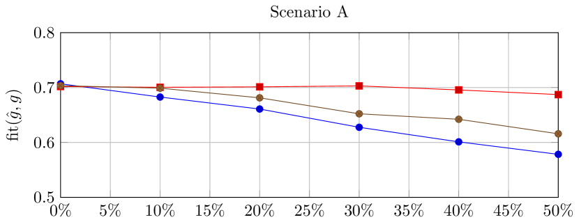
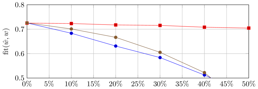
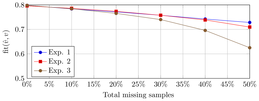
Figure 2: Plot of the median fit of the impulse response (top), the smoothed input (middle) and the smoothed output (bottom) over 500 MC runs, for increasing fractions of missing samples; In Exp.1 we remove input samples, in Exp.2 we remove output samples, in Exp.3 we remove input and output samples.

Unsolvable problems	0	3	5	16	27	40
Total missing samples	0%	10%	20%	30%	40%	50%

Table 2: Number of non-identifiable systems in Exp. 3 (out of 500)

Scenario B: Input noise

The input noise is Gaussian white noise. We consider values of the input noise variance between 0 (no noise) and 1 (same variance as the input), in increments of 0.2. The results are plotted in Figure 3. In this scenario, we compare the performance of the proposed method with a kernel-based identification method that does not account for input noise. We estimate the impulse response using the posterior mean $m$ from (17), with $\lambda$, $\beta$ and $\sigma_{y}^{2}$ estimated trough marginal likelihood, with all instances of $w$ replaced by the noisy measurements $u$.

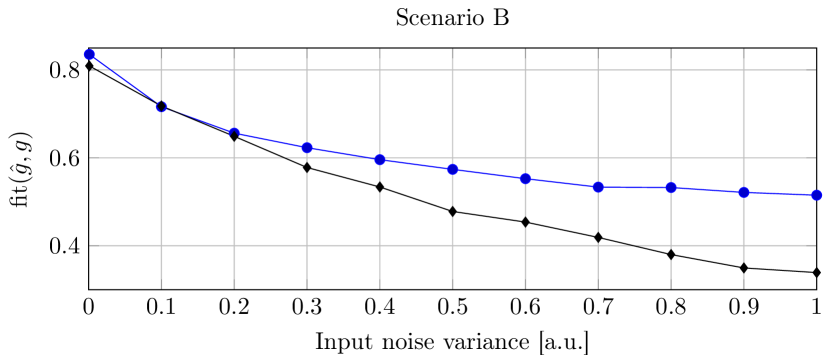
Figure 3: Plot of the median fit of the impulse response estimate over 500 MC runs, for increasing values of the input noise variance. We compare the proposed estimator (blue) with performance of an estimator that does not account for input noise (black).

7 Conclusions

In this paper we have presented a nonparametric kernel-based method for the identification of the impulse response of a linear systems in the presence of noisy and missing input-output data. The method relies upon a Gaussian regression framework, where the impulse response of the system is modeled as a Gaussian process with a suitable covariance matrix. Using an EB approach, we find the minimum mean-squared estimate of the impulse response. This estimate depends on the unknown noiseless input, as well as on the kernel hyperparameters and the noise variances. These quantities are estimated from the marginal likelihood of the data, obtained integrating out the impulse response. We have devised an iterative scheme that solves the marginal likelihood maximization in simple updates, and we have discussed the convergence properties of the algorithm. We have tested the method on a data bank of linear systems, where we have analyzed the degradation in performance for increasing amounts of missing data, and increasing noise variance on the input measurements. We have briefly addressed the question of identifiability; and simulations seem to validate our theoretical results, however, this aspect needs further study.

References

- [1] L. Ljung, System Identification, Theory for the User. Prentice Hall, 1999.
- [2] T. Söderström, “Errors-in-variables methods in system identification,” Automatica, vol. 43, no. 6, pp. 939–958, 2007.
- [3] R. Frisch, “Statistical confluence analysis by means of complete regression systems (university institute of economics, oslo, 1934, pp. 5–8),” in The Foundations of Econometric Analysis, pp. 271–273, Cambridge University Press, 1934.
- [4] B. D. Anderson, “Identification of scalar errors-in-variables models with dynamics,” Automatica, vol. 21, no. 6, pp. 709–716, 1985.
- [5] K. V. Fernando and H. Nicholson, “Identification of linear systems with input and output noise: the koopmans-levin method,” IEE Proc. D. Control Theory Appl., vol. 132, no. 1, pp. 30–36, 1985.
- [6] W.-X. Zheng and C.-B. Feng, “Unbiased parameter estimation of linear systems in the presence of input and output noise,” Int. J. Adapt. Control Signal Process., vol. 3, no. 3, pp. 231–251, 1989.
- [7] S. Beghelli, R. Guidorzi, and U. Soverini, “The frisch scheme in dynamic system identification,” Automatica, vol. 26, no. 1, pp. 171–176, 1990.
- [8] T. Söderström, U. Soverini, and K. Mahata, “Perspectives on errors-in-variables estimation for dynamic systems,” Signal Process., vol. 82, no. 8, pp. 1139–1154, 2002.
- [9] D. Fan and G. Luo, “Frisch scheme identification for errors-in-variables systems,” in Proc. IEEE Int. Conf. Cogn. Infor. (ICCI), pp. 794 – 799, 2010.
- [10] L. Ning, T. T. Georgiou, A. Tannenbaum, and S. P. Boyd, “Linear models based on noisy data and the frisch scheme,” SIAM Rev., vol. 57, no. 2, pp. 167–197, 2015.
- [11] E. Zhang and R. Pintelon, “Errors-in-variables identification of dynamic systems in general cases,” in Proc. IFAC Symp. System Identification (SYSID), vol. 48, pp. 309–313, 2015.
- [12] T. Söderström, “Identification of stochastic linear systems in presence of input noise,” Automatica, vol. 17, no. 5, pp. 713–725, 1981.
- [13] R. Diversi, R. Guidorzi, and U. Soverini, “Maximum likelihood identification of noisy input–output models,” Automatica, vol. 43, no. 3, pp. 464–472, 2007.
- [14] J. Schoukens, R. Pintelon, G. Vandersteen, and P. Guillaume, “Frequency-domain system identification using non-parametric noise models estimated from a small number of data sets,” Automatica, vol. 33, no. 6, pp. 1073–1086, 1997.
- [15] T. Söderström, M. Hong, J. Schoukens, and R. Pintelon, “Accuracy analysis of time domain maximum likelihood method and sample maximum likelihood method for errors-in-variables and output error identification,” Automatica, vol. 46, no. 4, pp. 721–727, 2010.
- [16] A. Isaksson, “Identification of arx-models subject to missing data,” IEEE Trans. Autom. Control, vol. 38, no. 5, pp. 813–819, 1993.
- [17] R. Pintelon and J. Schoukens, “Frequency domain system identification with missing data,” IEEE Trans. Autom. Control, vol. 45, no. 2, pp. 364–369, 2000.
- [18] R. Wallin and A. Hansson, “Maximum likelihood estimation of linear SISO models subject to missing output data and missing input data,” Int. J. Control, pp. 1–11, 2014.
- [19] I. Markovsky and R. Pintelon, “Identification of linear time-invariant systems from multiple experiments,” IEEE Trans. Signal Process., vol. 63, no. 13, pp. 3549–3554, 2015.
- [20] E. Zhang, R. Pintelon, and J. Schoukens, “Errors-in-variables identification of dynamic systems excited by arbitrary non-white input,” Automatica, vol. 49, no. 10, pp. 3032–3041, 2013.
- [21] Z. Liu, A. Hansson, and L. Vandenberghe, “Nuclear norm system identification with missing inputs and outputs,” Syst. Control Lett., vol. 62, no. 8, pp. 605–612, 2013.
- [22] I. Markovsky and K. Usevich, “Structured low-rank approximation with missing data,” SIAM J. Matrix Anal. & Appl., vol. 34, no. 2, pp. 814–830, 2013.
- [23] C. Williams and C. Rasmussen, Gaussian processes for machine learning. 2006.
- [24] G. Pillonetto and G. De Nicolao, “A new kernel-based approach for linear system identification,” Automatica, vol. 46, no. 1, pp. 81–93, 2010.
- [25] G. Pillonetto, F. Dinuzzo, T. Chen, G. D. Nicolao, and L. Ljung, “Kernel methods in system identification, machine learning and function estimation: A survey,” Automatica, vol. 50, pp. 657–682, mar 2014.
- [26] J. Maritz and T. Lwin, Empirical bayes methods. Chapman and Hall London, 1989.
- [27] G. Pillonetto and A. Chiuso, “A Bayesian learning approach to linear system identification with missing data,” in Proc. IEEE Conf. Decis. Control (CDC), pp. 4698–4703, 2009.
- [28] G. McLachlan and T. Krishnan, The EM algorithm and extensions, vol. 382. John Wiley and Sons, 2007.
- [29] C. F. J. Wu, “On the convergence properties of the EM algorithm,” Ann. Statist., vol. 11, pp. 95–103, mar 1983.
- [30] G. Bottegal, G. Picci, and S. Pinzoni, “On the identifiability of errors-in-variables models with white measurement errors,” Automatica, vol. 47, no. 3, pp. 545–551, 2011.
- [31] R. Wallin and A. Isaksson, “Multiple optima in identification of arx models subject to missing data,” EURASIP J. Adv. Signal Process., vol. 2002, no. 1, pp. 1–8, 2002.
- [32] T. Chen, L. Ljung, M. Andersen, A. Chiuso, F. Carli, and G. Pillonetto, “Sparse multiple kernels for impulse response estimation with majorization minimization algorithms,” in Proc. IEEE Conf. Decis. Control (CDC), pp. 1500–1505, 2012.