The surprising dynamics of a chain on a pulley: Lift-off and snapping

Abstract

The motion of weights attached to a chain or string moving on a frictionless pulley is a classic problem of introductory physics used to understand the relationship between force and acceleration. Here, we consider the dynamics of the chain when one of the weights is removed and, thus, one end is pulled with constant acceleration. This simple change has dramatic consequences for the ensuing motion: at a finite time, the chain ‘lifts off’ from the pulley and the free end subsequently accelerates faster than the end that is pulled. Eventually, the chain undergoes a dramatic reversal of curvature reminiscent of the crack, or snap, of a whip. We combine experiments, numerical simulations, and theoretical arguments to explain key aspects of this dynamical problem.

   

1 Introduction

When publishing the design of his machine in 1784, little could Atwood have known that, more than two centuries later, students would be asked to predict the outcome of his experiment. The problem, traditionally offered as an illustration of the principles of Newtonian mechanics, consists in deriving the acceleration $a$ of two masses $M>m$ subject to the action of gravity $g$ while attached to a massless and inextensible chain passing over a frictionless pulley. The well-known result is that

$$\mbox{\boldmath$a$}=\frac{M-m}{M+m}\mbox{\boldmath$g$}\,$$ (1)

for the heavier of the two, with the second having the opposite acceleration. Little attention has been paid to the seemingly trivial case in which both $m=0$ and the chain has a finite linear density. If the mass of the chain nevertheless remains small compared to $M$, then equation (1) immediately gives that the remaining mass falls with acceleration $a=g$. However, a simple experiment (see, for example, figure 1b) reveals that this apparent simplification actually has a dramatic effect on the resulting motion: the chain ‘lifts off’ from the pulley in a complex motion. This lift-off has some surprising features that we explore in detail in this paper. In particular, we show that the free end accelerates faster than the end that is being pulled by the mass: in this sense, the free end ‘beats’ the free fall of the mass. We also show that the chain eventually ‘snaps’ in a manner that is reminiscent of the crack of a whip[1, 2].

Thin filamentary structures are as important in applications as they are ubiquitous in nature and industry; examples range from macromolecules such as DNA [3] to the kilometric transoceanic cables laid on the ocean bed from telecommunication vessels [4]. On a human scale, textiles, hair and ropes are other examples of thin elongated structures in which one dimension greatly exceeds the two others (so that the objects may be modeled as one-dimensional). The thinness of such rod-like structures also makes them flexible so that they are frequently subject to large deformations in the three dimensional environment in which they evolve. This flexibility in shape in turn leads to rich bifurcation landscapes [5], striking pattern formation [6], and intricate dynamical behavior.

Despite the range of length scales and materials encountered, many filamentary structures are well modeled by the Kirchhoff equations for elastic rods [7]. A particularly interesting limit of these equations is the case of inextensible strings in which inextensible rods have negligible resistance to bending and twisting: their behaviour is dictated to a large extent by the geometric constraint of inextensibility. In fact, this constraint by itself is enough to give rise to complicated dynamics: while the simplest case of a straight string accelerating along its length may be understood by a simple application of Newton’s second law, any closed shape is a solution of the governing equations with any constant tangential velocity [8]. It is therefore the combination of acceleration and ‘turning a corner’ that gives rise to the most interesting dynamics. In particular, moving inextensible strings form surprisingly complicated shapes including arches [9] and the mesmerising ‘chain fountain’ [10, 11].

In this paper we consider the planar motion of a chain moving around a pulley subject to a constant acceleration at one end and free at the other end. We model the chain as an inextensible string in partial contact with a disk (the pulley) and investigate key features of the motion. This setup is perhaps the simplest geometry in which one can study how a string or chain ‘turns a corner’ since the curvature of this corner is simply that of the pulley. We first describe in some detail the different phenomena that are observed experimentally and then analyze the lift-off in detail by combining theoretical arguments with numerical simulations. Finally, we describe the snapping that is associated with the reversal of curvature that ultimately occurs close to the free end.

2 Statement of the problem and experimental observations

In the idealized setup of our problem, a mass $M$ is attached to the end of a chain of linear density (mass per unit length) $\rho_{\ell}$ placed around a circular pulley of radius $R$. The mass $M$ is released at time $t=0$ and subject to a constant acceleration $a$. The chain is initially held on the pulley with a known length of chain, $L$, hanging free from the first point of contact $C$ (see Fig 1a). In a typical experiment the total length of the chain is $L_{\text{end}}=2L+\pi R$.

The realization of this thought-experiment was carried out by using conventional ball and link chains purchased from the local do-it-yourself shop and hung over horizontal Pyrex beakers (Fisher Scientific) that were used as the frictionless pulley (the surface of the beaker being smooth, the chain slides over the surface with very little friction). The mass $M{\gg\rho_{\ell}L}$ is released at time $t=0$ resulting in an acceleration $a\approx g$. Although not restricted in any other way than by a frictionless contact with the pulley, the motion of the chain was observed to be planar, $i.e.$ the motion remains in the $xy-$plane normal to the axis of the pulley and containing the chain at $t=0$. In the subsequent modelling, we therefore assume that the motion remains planar throughout.

Figure 1: Experiments using ball chains. (a) Experimental setup: the free fall of a mass $M$ forces a chain with initial hanging length $L=54\mathrm{~{}cm}$ to slide around a glass cylinder of radius $R=4\mathrm{~{}cm}$. The initial length $L$ of the hanging part denotes the section of chain from the free end $s=0$ to the first contact point with the cylinder $C$ before the mass is dropped (which occurs at $t=0$). The vectors $(\mbox{\boldmath$t$},\mbox{\boldmath$n$})$ denote the tangent and the normal of the chain, respectively. (b) Time sequence ($\Delta t=2.5\mathrm{~{}ms}$) of the chain dynamics successively lifting up from pulley (from $t=t_{\mathrm{LO}}$ onwards) showing that a ballooning arch develops before the chain eventually ‘snaps’ at a time $t=t^{*}$ (reverses its curvature dramatically).

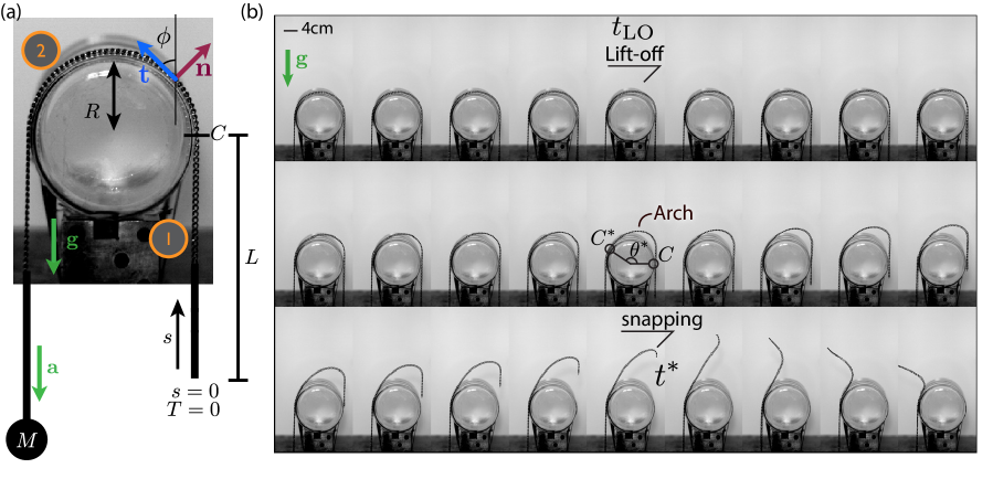
Typically, the time evolution of the chain passes through three, qualitatively different, phases shown in figure 1b:

• For $0\leq t<t_{\mathrm{LO}}$ the chain follows the dynamics that might naively be expected: it moves around the pulley at the speed that is imposed by the accelerating mass.

• At a time $t=t_{\mathrm{LO}}$ the chain starts to partially lose contact with the pulley, lifting off so that for $t>t_{\mathrm{LO}}$ the hanging part of the chain goes faster than the rest of the chain. Due to the excess length of the chain, an arch forms between points $C$ and $C^{*}(t)$ defining an angle $\theta^{*}(t)$ (see figure 1b).

• After the free end goes past the last contact point $C$ (first image of the last row in figure 1b) the arch flares up, its curvature increasing rapidly until the free end eventually snaps at time $t=t^{*}$ (the curvature there changes sign).

To complement our experiments, numerical simulations were carried out using the Discrete Elastic Rod method, which provides a discretization of the equations of motion for thin elastic rods using a Lagrangian formulation [12]. This method, and its counterpart for thin viscous threads, have been used and validated previously [13, 14]. In the simulations, we use a string model, i.e. the bending and twisting stiffnesses are both set to zero so that the Kirchhoff equations [7] simplify to the conservation of linear momentum:

$$\frac{\partial(T\mbox{\boldmath$t$})}{\partial s}+\rho_{\ell}\mbox{\boldmath$g$}+P\mbox{\boldmath$n$}=\rho_{\ell}\frac{\partial\mbox{\boldmath$v$}}{\partial t},$$ (2)

and inextensibility

$$\left|\frac{\partial\mbox{\boldmath$x$}(s,t)}{\partial s}\right|=1,$$ (3)

where $\mbox{\boldmath$x$}(s,t)$ is the centre-line of the chain as a function of the arc length $s$ and time $t$, $\mbox{\boldmath$t$}(s,t)=\frac{\partial\mbox{\boldmath$x$}(s,t)}{\partial s}$ and $\mbox{\boldmath$n$}(s,t)$ are the unit tangent and normal vectors to the chain axis, respectively (see Figure 1a). Further, the variables $T(s,t)$ and $\mbox{\boldmath$v$}(s,t)=\frac{\partial\mbox{\boldmath$x$}(s,t)}{\partial t}$ denote the tension and velocity of the chain, and $P(s,t)$ represents the (frictionless) reaction from the pulley on the chain, such that $P=0$ whenever there is no contact. This frictionless contact with the pulley is implemented numerically using a geometrical method, i.e. by alternating dynamic steps that ignore contact forces, with projection steps in which the configuration is projected onto the manifold of admissible configurations.

We close the differential problem (2)-(3) using the boundary conditions at the two ends of the chain. Namely, the free end of the string is stress free and we prescribe the acceleration $a$ of the chain’s end attached to the mass in our experiments, that is:

$$T(0,t)=0$$ (4)

$$\dot{\mbox{\boldmath$v$}}(L_{\text{end}},t)=-a\,\mbox{\boldmath$e$}_{y}$$ (5)

where $\mbox{\boldmath$e$}_{y}$ is in the vertical direction and $L_{\text{end}}=2L+\pi R$ is the arc-length corresponding to the point where the mass is attached.

Figure 2: Numerical simulations: (a) Comparison between the chain shape observed experimentally (images in the background) and the prediction of numerical simulations (overlaid dashed curve). Here there are no adjustable parameters ($L=54\mathrm{~{}cm}$, $R=4\mathrm{~{}cm}$, time between two frames $\Delta t=0.9\mathrm{~{}ms}$). (b) At each instant before snapping, the chain may be divided into four zones. (c) Plot of the curvature $\kappa$ (dashed curve) and the chain speed $v$ (solid curve) as functions of the arc length. (d) A numerical reconstruction of the tension $T$ within the chain shows that it varies linearly with arc length in regions (I), (III) & (IV). Region (II) bridges regions (I) and (III), each of which is characterized by a different acceleration. For comparison, the dashed line shows the tension as a function of arc length in the idealized solution with uniform and constant acceleration $a$ where lift-off is prevented (this artificial solution would give rise to a negative contact pressure).

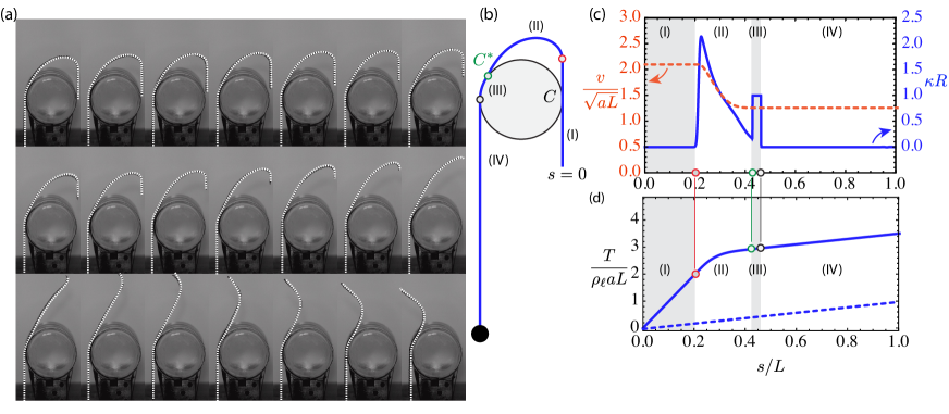
Figure 2 shows a direct comparison between experiments and numerical simulations without any adjustable parameter. The favorable agreement between the two validates the approximations made in modelling the chain as a string that is driven at constant acceleration (our experiments are in fact conducted with a constant force $M\mbox{\boldmath$g$}$ but the two methods are approximately equivalent since $\rho_{\ell}L\ll M$). Of particular interest is the possibility offered by the simulations to access the successive space derivatives of the basic physical variables (such as curvature) with controllable time resolution covering long periods of time. Additionally, physical quantities that are otherwise challenging to measure experimentally, such as the tension within the chain, are readily available from simulations.

At any given time before the chain snaps ($0<t<t^{*}$), the chain may be divided into four regions: (I) and (IV) denote the two straight, vertical parts, respectively, (II) denotes the part of the chain not in contact with the pulley and (III) the contact region. For example, in figure 2b-d, only a small portion of the chain (III) remains in contact with the pulley. In this region the chain’s speed is prescribed by the free fall of the mass, as in region (IV). In region (I), the chain moves significantly faster than the imposed acceleration, while remaining perfectly straight and tangential to the pulley. In addition, the tension in the chain is larger than if the lift-off were artificially suppressed (shown as a dashed line in figure 2d). The area (II) bridges the areas (I) and (III)-(IV) and their corresponding physical quantities, resulting in a ballooning shape (see figure 2).

The length of the chain that is initially hanging freely, $L$, turns out to play an important role in the problem and, therefore, we use $L$ as the length scale of the problem. It is then natural to use the quantity $(L/a)^{1/2}$ as the time scale of the problem. If the acceleration of the freely hanging part of the chain were to remain at $a$ throughout the motion, the length of the chain hanging beneath the point C then shrinks to zero at a time $t=\sqrt{2L/a}$.

From the 6 dimensional quantities of interest, we identify three dimensionless parameters:

$$\pi_{1}=\rho_{\ell}L/M,\,\,\,\,\pi_{2}=R/L,\,\,\,\,\text{and}\,\,\,\,\pi_{3}=g/a.$$ (6)

In our experiments $M$ is chosen such that $\pi_{1}\ll 1$; $\rho_{\ell}$ therefore enters in the problem as a multiplying factor for forces only. The value of $\pi_{2}$ may easily be varied experimentally by varying the radius of the pulley or, more simply, by varying the length of chain that initially hangs freely. By contrast, varying $\pi_{3}$ is more difficult. Our experiments are always performed with $a=g$ and hence $\pi_{3}=1$. However, the inclusion of a body force acting on the chain complicates some of the analysis without changing the qualitative behaviour, as shown in figure 2. Therefore, in much of the analysis we shall neglect the acceleration due to gravity, i.e. we assume $\pi_{3}=0$. Experimentally, this case could be obtained by placing the chain, pulley and the mass on a smooth horizontal surface: at $t=0$, the mass is then pushed off the table into the air [15] and allowed to fall under gravity so that the acceleration of the chain is $a=g$ but the effective gravity acting directly on the chain vanishes. In the simulations, the value of $\pi_{3}$ is set to 1 or 0 depending on whether the results are to be compared with experiments or with our analysis.

3 Prior to lift-off

We consider a pulley of radius $R$ around which a chain with linear density $\rho_{\ell}$ is hung. We begin by including gravity as a body force, though later we will neglect it to simplify the ensuing calculations. Initially, the length of chain between the free end (at arc-length position $s=0$) and the chain’s first point of contact with the pulley is $L$ (i.e. the point C in figure 1 has arc-length coordinate $s=L$ at $t=0^{-}$).

At $t=0^{+}$, the end at arc length $s=L_{\text{end}}$ is pulled with constant acceleration $a$. Assuming that the chain remains in contact with the pulley, $\mbox{\boldmath$v$}=v\mbox{\boldmath$t$}$, and projecting (2) onto the tangential and normal directions, and then using the Frenet formula $\partial\mbox{\boldmath$t$}/\partial s=-\kappa\mbox{\boldmath$n$}$ with $\kappa$ the curvature, we find that

$$\frac{\partial T}{\partial s}-\rho_{\ell}g\cos\phi = \rho_{\ell}\frac{\partial v}{\partial t}$$ (7)

$$-{T\kappa}-\rho_{\ell}g\sin\phi+P = -\rho_{\ell}{v^{2}\kappa},$$ (8)

where $\phi$ is the angle between the local tangent to the chain and the upward pointing vertical and $\kappa=\partial\phi/\partial s$ is the curvature. In particular, while the chain remains in contact with the pulley, $t<t_{\mathrm{LO}}$, we know that

$$\phi(s,t)=\begin{cases}0,&0\leq s<s_{C}\\ \frac{s-s_{C}}{R},&s_{C}\leq s<s_{C}+\pi R\\ \pi,&s_{C}+\pi R\leq s\end{cases}$$ (9)

where

$$s_{C}(t)=L-at^{2}/2$$ (10)

is the arc-length position of the first contact point between the pulley and the chain (the point labelled C in figure 1). In the hanging part $\phi(s,t)=0$, and so, integrating (7) subject to $T(0,t)=0$, we find that the tension $T$ may be written:

$$T(s,t)=\rho_{\ell}(a+g)s,\,\,\,s\in[0,s_{C}]$$ (11)

In the region where the chain is in contact with the pulley, (7) leads to

$$T(s,t)=\rho_{\ell}as+\rho_{\ell}gR\sin\phi+C_{1},\,\,s\in[s_{C},s_{C}+\pi R]$$ (12)

where the constant of integration $C_{1}=\rho_{\ell}g\,s_{C}$ is found by requiring the tension to be continuous at $s=s_{C}$.

In the freely hanging portion of the chain, $\eqref{k2}$ is identically satisfied by $P=0$. Elsewhere, (8) can be viewed as an equation for the reaction of the pulley on the chain required for this motion to occur. From a simple rearrangement, we find that

$$P=-\rho_{\ell}\frac{v^{2}}{R}+2\rho_{\ell}g\sin\phi+\frac{1}{R}\rho_{\ell}(as+gs_{C}),\quad s\in[s_{C},s_{C}+\pi R].$$ (13)

Note that $P$ is a function of arc length $s$ and time $t$ through the angle $\phi$ and arc length of the contact point, $s_{C}(t)$, in addition to the explicit dependence on $s$. The minimum value of $P$ at any particular time $t<t_{\mathrm{LO}}$ is attained at $s=s_{C}$:

$$P_{\mathrm{min}}(t)=\rho_{\ell}\bigl{[}s_{C}(a+g)-v^{2}\bigr{]}/R=\rho_{\ell}\bigl{[}(a+g)L-\tfrac{1}{2}at^{2}(3a+g)\bigr{]}/R.$$ (14)

The key to understanding why lift-off occurs is held by the expression for the smallest reaction force $P_{\mathrm{min}}(t)$ (14). At sufficiently early times $P_{\mathrm{min}}>0$, and the contact pressure is everywhere positive (it prevents the chain from penetrating the pulley). However, $P_{\mathrm{min}}$ vanishes at a time $t=t_{\mathrm{LO}}$ given by

$$t_{\mathrm{LO}}=\sqrt{\frac{2L(a+g)}{a(3a+g)}}=\sqrt{\frac{2\,L}{a}}\sqrt{\frac{1+\pi_{3}}{3+\pi_{3}}},$$ (15)

and then becomes negative. For time $t>t_{\mathrm{LO}}$, the assumption (9) that the string is in contact with the pulley over half a circle breaks down, as it predicts a negative pressure (an adhesive force would be required to maintain contact). The negative values of $P$ are first attained in the neighbourhood of $C$, which suggests that lift-off takes place there. At time $t=t_{\mathrm{LO}}$, the length of the hanging chain is

$$s_{C}^{\mathrm{LO}}=s_{C}(t_{\mathrm{LO}})=\frac{2a}{3a+g}L=\frac{2}{3+\pi_{3}}L.$$ (16)

In (15), $t_{\mathrm{LO}}$ is less than the time $\sqrt{2L/a}$ when the hanging part (I) shrinks to a point the mathematical solution (9) ignoring the lift-off. This confirms that the hanging part (I) has a finite length when the lift-off takes place. This is also consistent with $s_{C}^{\mathrm{LO}}=s_{C}(t_{\mathrm{LO}})>0$.

Apart from factors obviously required by dimensional analysis, both (15) and (16) appear to depend only on the ratio $\pi_{3}=g/a$ of the acceleration due to gravity to the imposed acceleration. They do not depend on the dimensionless group $\pi_{2}=R/L$ involving the size of the pulley. Furthermore, we note that in the limit of zero gravity, $\pi_{3}=0$, one third of the original hanging chain has passed around the pulley with two-thirds still hanging; when pulling the chain using a heavy mass in free fall, i.e. imposing $\pi_{3}=1$, then one-half of the original hanging chain has passed around the pulley with one-half still hanging. Here, incorporating gravity makes a quantitative, but not qualitative, difference; either way, an appreciable fraction of the initially hanging chain remains below the first contact point C.

From the above argument, we also gain some intuition into why the chain lifts off: the tension at the contact point $s_{C}(t)$ is decreasing with time (because the length of hanging chain is decreasing) while the tension required to turn the chain around the pulley increases (because the chain is moving faster and faster). Lift-off occurs when the excess tension in the chain due to the hanging length is ‘used up’.

4 Lift-off

Figure 3: Experimental values of the time at which lift off occurs, $t_{\mathrm{LO}}$, plotted as a function of the chain length $L$. This data, gathered with pulleys of radius ranging from $R=2.5\mathrm{~{}cm}$ to $R=7.5\mathrm{~{}cm}$ and two types of chain, collapses on a single master curve. The prediction derived in §3 (see eq. (15)) is verified within $10\%$ (the solid curve corresponds to $t_{\mathrm{LO}}\simeq 1.1\sqrt{L/g}$) . In these experiments, $a=g$, i.e. $\pi_{3}=1$.

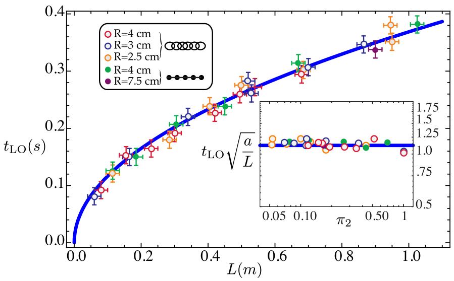
The prediction for the lift-off time, (15), presents a natural test of the model assumptions, in particular with regard to our neglect of the bending stiffness of the chain and the assumption of a frictionless contact between chain and pulley. Experiments were performed with $a=g$ (i.e. $\pi_{3}=1$) and a number of different pulley sizes and initial hanging lengths (i.e. varying $\pi_{2}$). As shown in figure 3, we find reasonable agreement between the theoretical prediction for $t_{\mathrm{LO}}$ and that measured experimentally. In particular, experiments confirm the result that the size ratio $\pi_{2}=R/L$ does not affect the onset of lift-off. We also found that the value of $t_{\mathrm{LO}}$ is insensitive to the type of chain used (ball chains and link chains give the same results).

However, we note that the onset of lift-off is difficult to assess accurately in experiments owing to its slow initial dynamics (to be discussed in detail in § 5); it is therefore natural that experimental values of $t_{\mathrm{LO}}$ are slightly larger that theoretically predicted (though they remain within 10% of the theoretical value). Furthermore, the favorable agreement between experiments and numerical solution of the full model, which neglects any source of dissipation, shown in figure 2a suggests friction cannot be the cause of the discrepancy.

5 Behaviour just after lift-off

We now turn our attention to the early phase of the motion, just after lift-off. In this phase, our experiments and numerical simulations show that the chain ‘balloons’ off the pulley (see figure 1b). For simplicity, we shall henceforth neglect the role of gravity, i.e. we set $\pi_{3}=0$. This analysis is conducted hand in hand with numerical simulations for $\pi_{3}=0$, but these results should not be compared with experiments (for which $\pi_{3}=1$). In Appendix A we consider how the results of this section change when $\pi_{3}\neq 0$; this analysis shows that the presence of gravity makes quantitative, rather than qualitative, changes to the motion around lift-off.

5.1 Velocity after lift-off

Figure 4: Behavior just after lift-off for $\pi_{3}=0$ (imposed acceleration at endpoint is $a=0.5$, $g=0$, $R=1$ and $L=4\pi$; the simulation timestep is $\Delta t=15\times 10^{-4}$ and the mesh size is $\Delta s=6.3\times 10^{-3}$). (a) The speed of the hanging part of the chain for $g=0$ from numerical simulations (dotted blue curve) compared to the imposed velocity at the pulling end, $v=at$, (dashed line) and the prediction of eq. 19 (solid orange curve). Inset: Error $\delta$ between the estimate (19) for $v_{\mathrm{hang}}$ and the numerical data, shows that the expansion for $t-t_{\mathrm{LO}}\ll t_{\mathrm{LO}}$ in (20) is correct at $O(t-t_{\mathrm{LO}})^{2}$. (b) $\Delta s$ denotes the length of chain that has lost contact with the pulley for $t>t_{\mathrm{LO}}$. The corresponding angle is $\theta^{*}$ representing a region on the pulley of length $R\theta^{*}$. The excess length $\Delta L$ is defined as the difference between these two quantities $\Delta L=\Delta-R\theta^{*}$ (c) The value of the relative excess length $\Delta L/L$ (solid) as predicted by equation (22) compares favourably with numerical data (dots); in particular the scaling prediction $\Delta L/L\sim(t-t_{\mathrm{LO}})^{3}$ is borne out by the data.

The numerical simulations of the complete theoretical model (eqs 2-5) and experiments both suggest that the portion of the chain that is freely hanging at the instant of first lift-off (i.e. $0\leq s<s_{C}(t_{\mathrm{LO}})$) remains straight (within numerical accuracy) in the immediate aftermath of lift-off. We therefore attempt to repeat the calculation of §3 but this time we treat the acceleration in this straight portion, $\dot{v}_{\mathrm{hang}}(t)$, as an unknown. Motivated by numerical observations, we assume that the length of the straight portion of the chain is precisely the hanging length of the chain at $t_{\mathrm{LO}}$, namely $s_{C}(t_{\mathrm{LO}})$, which we denote by $s_{C}^{\mathrm{LO}}$ as in (16).

Setting $g=0$ in (2), and focusing on the straight, hanging part (zero curvature), and integrating we find that:

$$T=\rho_{\ell}\dot{v}_{\mathrm{hang}}s,\quad 0\leq s\leq s_{C}^{\mathrm{LO}}$$ (17)

where the length of the straight portion $s_{C}^{\mathrm{LO}}=L-\tfrac{1}{2}at_{\mathrm{LO}}^{2}$. To close the problem, we note that at the end of this straight portion, the radius of curvature must change to some finite value (by construction), and further that there is no reaction force (since at this point the chain is no longer in contact with the pulley). Substituting these results into (8), we then have that $T(s_{C}^{\mathrm{LO}},t)=\rho_{\ell}v_{\mathrm{hang}}^{2}$ and hence, after combining with (17), that

$$\dot{v}_{\mathrm{hang}}(t)=\frac{v_{\mathrm{hang}}^{2}(t)}{s_{C}^{\mathrm{LO}}}.$$ (18)

Integrating (18) subject to the initial condition $v_{\mathrm{hang}}(t_{\mathrm{LO}})=at_{\mathrm{LO}}$, we find that

$$v_{\mathrm{hang}}(t)=\frac{2}{3}\,\frac{L}{2t_{\mathrm{LO}}-t}=a\,t_{\mathrm{LO}}\,\left(2-\frac{t}{t_{\mathrm{LO}}}\right)^{-1}\textrm{.}$$ (19)

This simple approximation predicts that the velocity of the hanging portion of the chain diverges as $t\to 2t_{\mathrm{LO}}$. However, the argument above only holds in the immediate aftermath of lift-off, $t-t_{\mathrm{LO}}\ll t_{\mathrm{LO}}$. In the simulations, the reversal of curvature actually occurs at a time $t^{*}\approx 1.365\sqrt{L/a}\approx 1.67t_{\mathrm{LO}}$ (see figure 7b-c), which is earlier than that predicted by (19).

The Taylor expansion of (19) for $t-t_{\mathrm{LO}}\ll t_{\mathrm{LO}}$ reads

$$v_{\mathrm{hang}}(t)=a\,t_{\mathrm{LO}}\,\left[1+\frac{t-t_{\mathrm{LO}}}{t_{\mathrm{LO}}}+\left(\frac{t-t_{\mathrm{LO}}}{t_{\mathrm{LO}}}\right)^{2}+O\left(\frac{t-t_{\mathrm{LO}}}{t_{\mathrm{LO}}}\right)^{3}\right].$$ (20)

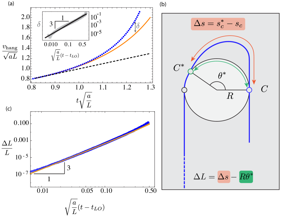
The first two terms in in the square bracket combine to give $at$, which is the imposed pulling velocity: the correction to the imposed constant acceleration is given by the following term and occurs at order $(t-t_{\mathrm{LO}})^{2}$. In figure 4a, we observe that our numerical results for the velocity are in good agreement with the prediction of eq. (19) for times close to $t_{\mathrm{LO}}$ but then deviate with an error $\delta$ that is cubic in $t-t_{\mathrm{LO}}$. This cubic error confirms that the first correction to the constant acceleration motion, namely the term of order $(t-t_{\mathrm{LO}})^{2}$ in (20), is correct.

By differentiating (19) with respect to time, we obtain an expression for the excess acceleration of the free part of the chain

$$\Delta a=\dot{v}_{\mathrm{hang}}-a=a\left[\frac{t_{\mathrm{LO}}^{2}}{(2t_{\mathrm{LO}}-t)^{2}}-1\right],$$ (21)

which is positive for all $t>t_{\mathrm{LO}}$. Thus, even though the free end is not subject to external forces, it accelerates faster than the end that is actually subject to the imposed (constant) acceleration.

A quantity of interest is the arc-length of the region over which the chain has lost contact with the pulley for $t>t_{\mathrm{LO}}$, which we denote by $\Delta s$ (see figure 4b). The above calculation does not give us enough information to determine this quantity. However, the result for $v_{\mathrm{hang}}$, (19), can be used to determine the excess length of chain that has lost contact with the pulley, i.e. the difference between the length of chain that has lifted off the pulley, $\Delta s(t)$, and the arc length of the pulley from which it has lifted off, $R\theta^{*}(t)$, with $\theta^{*}(t)$ the angle subtended between the two contact points C and C^∗ (see figure 4b). Denoting this quantity by $\Delta L(t)=\Delta s(t)-R\theta^{*}(t)$ we find that

$$\Delta L(t)=\int_{t_{\mathrm{LO}}}^{t}\left[v_{\mathrm{hang}}(t^{\prime})-at^{\prime}\right]~{}\mathrm{d}t^{\prime}=\frac{2L}{3}\log\left(\frac{t_{\mathrm{LO}}}{2t_{\mathrm{LO}}-t}\right)-\frac{a}{2}(t^{2}-t_{\mathrm{LO}}^{2}).$$ (22)

We emphasize that this calculation does not allow us to determine $\Delta s$ and $R\theta^{*}$ separately, but only their difference. The Taylor series of $\Delta L(t)$ for $t-t_{\mathrm{LO}}\ll t_{\mathrm{LO}}$ reveals that

$$\Delta L(t)\approx a{(t-t_{\mathrm{LO}})^{3}\over 3t_{\mathrm{LO}}},$$ (23)

i.e. the excess length grows only relatively slowly after the start of lift-off. Note that the appearance of a leading-order behaviour at order $(t-t_{\mathrm{LO}})^{3}$ here is consistent with our earlier finding that the correction to the speed of motion is at order $(t-t_{\mathrm{LO}})^{2}$ in (20), since we have integrated this quantity in time.

Comparison of the predictions of this analysis, (19) and (23), with the numerical solution of the fully nonlinear problem (see figure 4) shows that these expressions are asymptotically correct immediately after lift-off, $t-t_{\mathrm{LO}}\ll t_{\mathrm{LO}}$, and validates the underlying assumption (that the hanging portion of the chain simply accelerates vertically upwards).

5.2 Characteristics

Figure 5: The parameter space $(t\sqrt{a/L},s/L)$ is mapped with the characteristics of the system, color coded as functions of the direction of propagation (given by the sign of $\mathrm{d}s/\mathrm{d}t$ in this plot). The time evolution of the position of the contact point $C$, obtained analytically before $t_{\mathrm{LO}}$ and numerically for $t>t_{\mathrm{LO}}$, is shown by solid blue curve. The envelope of characteristics emitted from $C$ at $t=t_{\mathrm{LO}}$ is highlighted by the shaded area. (The simulation timestep is $\Delta t=15\times 10^{-4}$ and the mesh size is $\Delta s=6.3\times 10^{-3}$. Imposed acceleration at endpoint is $a=0.5$, $g=0$, $R=1$ and $L=4\pi$).

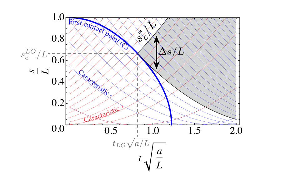
We now proceed to explain the size of the region of lift-off as a function of time. We show that the point of contact $C^{*}(t)$, as defined in fig 4b, follows a characteristic of the wave equation describing the evolution of the small perturbations to the motion of the string. In other words, the motion of $C^{*}(t)$ can be viewed as a traveling front produced by the initial lift-off at $t_{\mathrm{LO}}$. To do so, we now consider the length of chain $\Delta s$ that makes up the ‘ballooning’ arch forming after lift-off. This length is defined to be $\Delta s(t)=s_{c}^{*}-s_{c}$, where $s_{c}$ and $s_{c}^{*}$ correspond to the arc-length coordinate of the contact points $C$ and $C^{*}$, respectively (see figure 4b).

For times close to $t_{\mathrm{LO}}$, lift-off takes place but it is mild; as a result, this lift-off can be described by $(i)$ extending beyond $t_{\mathrm{LO}}$ the solution maintaining contact with the upper half of the pulley (base solution) and $(ii)$ perturbing it to remove any negative contact pressure. The equations governing the perturbation are obtained by a standard linearization, and are linear wave equations. In these wave equations, the wave speed $c=\sqrt{T/\rho_{\ell}}$ is both time and space-dependent (recall that $T=T(s,t)$). Assuming that the tension remains close to its value prior to lift-off, i.e. $T\approx\rho_{\ell}as$ as derived in eq.(11), we have $c=\sqrt{as}$, and the characteristics of the wave equation satisfy

$$\frac{\mathrm{d}s}{\mathrm{d}t}=\pm\sqrt{as}.$$ (24)

yielding the expansion waves depicted in figure 5.

When lift-off occurs, the chain is locally freed from the pulley at the point $s_{C}^{\mathrm{LO}}$ and this information propagates within the envelope formed by the two characteristics that depart from this point in the $(t,s)$ plot. Within this region, the tension in the chain is altered, i.e. the tension of the true solution does not match exactly that predicted by the base solution that ignores lift-off; beyond this region, information can only propagate at the wave speed at the edges, which is, by construction, given by the tension just before lift off. The limited propagation speed of information about lift-off results in the formation of an arch from the point $C$ to a second contact point $C^{*}$ (see figure 4b). We hypothesize that the length of the arch $\Delta s(t)=s_{c}^{*}-s_{c}$ is simply the width of the envelope formed by the two characteristics that originate from $C$ at $t=t_{\mathrm{LO}}$ (see figure 5). Deriving $\Delta s$ from eq.(24) yields

$$\Delta s=2\sqrt{\frac{2}{3}}\sqrt{aL}(t-t_{\mathrm{LO}}).$$ (25)

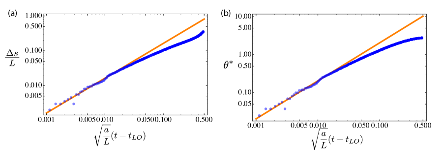
We use numerical simulations to test the estimate (25). As shown in figure 6a the agreement between the two is asymptotically correct immediately after lift-off (with the correct prefactor). This indicates that the propagation of lift-off front is indeed limited by the rate at which the perturbations can travel through the string. This argument correctly accounts for the short times dynamics, $\Delta s\sim(t-t_{\mathrm{LO}})$.

We also note that $\theta^{*}$, the angle from $C$ to $C^{*}$ defined in figure 5b, follows the same scaling law and agrees well with equation (25). Indeed, recall that $\Delta L=\Delta s-R\theta^{*}$; for $t-t_{\mathrm{LO}}\ll 1$, we have shown $\Delta L\sim(t-t_{\mathrm{LO}})^{3}$ in equation (23) and $\Delta s\sim(t-t_{\mathrm{LO}})$ above, it follows that $\Delta s$ and $R\,\theta^{*}$ must be equal to leading order in $(t-t_{\mathrm{LO}})$, i.e. $\theta^{*}\sim\Delta s/R$ as checked numerically in figure 6b.

Figure 6: Arch structure for $\pi_{3}=0$. (a) The evolution of $\Delta s/L$ with time following lift-off determined numerically (blue dots) and compared to the theoretical expression in (25) (orange solid line). (b) Test of the prediction $\theta^{*}\sim\Delta s/R$ derived at the end of §5. In both cases the numerical data corresponds to a simulation with timestep $\Delta t=15\times 10^{-4}$ and the mesh size $\Delta s=6.3\times 10^{-3}$. Imposed acceleration at endpoint is $a=0.5$, $g=0$, $R=1$ and $L=4\pi$.

6 Snapping

We now describe the kinematics of the free end during snapping. Let $\phi(s,t)$ be the angle between the tangent $t$ and the upward pointing vertical axis. We define the curvature $\kappa(s,t)=\partial\phi(s,t)/\partial s$ (recall that the free end corresponds to $s=0$). We define snapping as a sudden change in maximal curvature of the chain as depicted in figure 7a-b,

Figure 7: Snapping for $\pi_{3}=0$: (a) Shapes of the chain right before and after snapping occurs. The angle $\phi(s,t)$ separates the tangent $\mbox{\boldmath$t$}(s,t)$ and the the upward pointing vertical axis so that $\kappa(s,t)=\partial\phi(s,t)/\partial s$, where $\kappa$ is the curvature of the chain. (b) The maximal curvature of the chain $\kappa_{M}$ (attained at position $s_{M}$) as a function of time and (c) the velocity of the free end of the chain compared to the constant acceleration that drives the motion. The grey bands indicate the snapping time. (The simulation timestep is $\Delta t=15\times 10^{-4}$ and the mesh size is $\Delta s=6.3\times 10^{-3}$. Imposed acceleration at endpoint is $a=0.5$, $g=0$, $R=1$ and $L=4\pi$)

which shows the time evolution of the largest curvature of the chain, $\kappa_{M}$. We observe that the arc-length position $s_{M}$ at which this maximum curvature is observed travels towards the free end of the chain as snapping approaches, as shown in figure 7b. During snapping, $\kappa_{M}$ has a singular behavior as well: the curvature strongly increases and changes sign, as shown in the last three configurations in figure 7a and in figure 7b. Note that for real ropes this singularity will be regularized by their finite bending stiffness . Therefore, the singular behavior predicted by our string model may be seen as the ’outer solution’ of a regularized model. Note that snapping is associated with a rapid increase of the free end velocity as illustrated in figure 7c. These features are similar to what occurs in a cracking whip [1] and a falling chain [16, 17, 18, Grewal2011].

Let us denote by $t^{*}$ the time of snapping, defined as the time where the curvature diverges near the free end. For optimal accuracy, we analyze the snapping dynamics based on simulations having a relatively large value of $\pi_{2}=R/L=\frac{1}{2\pi}$. This allows us to use a fine and uniform spatial discretization of the string. To ease the comparison between this specific simulation and the rest of our results, we introduce a non-dimensionalisation with respect to the space and time scales of the problem, namely $L$ and $\sqrt{L/a}$. Dimensionless quantities are denoted by a bar, such as $\overline{t}^{*}=t^{*}/\sqrt{L/a}$. The dimensionless snapping time $\overline{t}^{*}$ is a function of $\pi_{2}$ and $\pi_{3}$; in the forthcoming analysis, we focus on the particular case $\pi_{2}=1/(2\pi)$ and $\pi_{3}=0$.

To measure the divergence of curvature from the simulations, we use a curvature norm that is intended to capture the largest value of curvature,

$$\overline{K}(t)=\left(\int_{0}^{1}\left(\overline{\kappa}(\overline{s},\overline{t}\,)\right)^{p}\,\mathrm{d}\overline{s}\right)^{\frac{1}{p-1}}\textrm{,}$$ (26)

where $p\geq 2$ is an integer. The value of the integer $p$ that is used results from a trade-off: one should use values of $p$ as large as possible, and $\overline{K}$ will then accurately capture the maximum curvature; on the other hand, if $p$ is too large then $\overline{K}$ fluctuates significantly as a result of discretization errors. In the following, we take $p=6$; we have verified that the results are unchanged for $p=8$.

We begin by assuming that as the singularity at $\overline{t}=\overline{t}^{*}$ is approached, the curvature diverges according to a power law $\overline{\kappa}\sim(\overline{t}^{*}-\overline{t})^{-\alpha}$, for some exponent $\alpha$ to be determined, on a region of size $\sim 1/\overline{\kappa}$. The region of divergence contributes an amount $\sim(\overline{t}^{*}-\overline{t})^{-(p-1)\,\alpha}$ to the integral in equation (26): as soon as $\alpha(p-1)>0$, this contribution makes the integral diverge at the time of snapping $\overline{t}^{*}$ and $\overline{t}^{*}$ can be identified from a numerical plot of $\overline{t}$ as a function of time—the condition $\alpha(p-1)>0$ is indeed satisfied as $p=6$ and $\alpha>0$, see below. One can check that the quantity $\overline{K}(t)$ diverges as $\overline{K}\sim(\overline{t}^{*}-\overline{t})^{-\alpha}$: a numerical plot of $\overline{K}$ versus $\overline{t}$ yields the exponent $\alpha$ as well, independently of the particular value of $p$ chosen in the definition of $\overline{K}$.

The snapping time $\overline{t}^{*}$ and the exponent $\alpha$ entering in the power law $\overline{K}(t)\sim|t-t^{*}|^{-\alpha}$ are best determined from the simulations by plotting the quantity

$$\left(\frac{\mathrm{d}(\ln\overline{K})}{\mathrm{d}\overline{t}}\right)^{-1}\sim\frac{\overline{t}^{*}-\overline{t}}{\alpha}$$ (27)

as a function of $\overline{t}$, see figure 8a.

Figure 8: Searching for self-similar solutions in the snapping (for this particular simulation, the linear mass is $\rho_{\ell}=5$ and the radius of pulley is $R=1$ and $L=2\pi$ such that $\pi_{2}=R/L=1/(2\pi)$. There is no gravity and no bending rigidity. The simulation timestep is $\Delta t=2\times 10^{-4}$ and the mesh size is $\Delta s=3.14\times 10^{-3}$. Imposed acceleration at endpoint is $a=0.5$). (a) Identifying the singularity exponent $\alpha$ for the curvature and the critical time $\overline{t}^{*}$ using the quantity $\overline{K}(\overline{t})$ defined in (26). From our numerical simulations we find that $(\alpha,\overline{t}^{*})=(0.659,1.41531)$ (red dashed line). (b) These values may be checked in a standard log-log plot. The wells are numerical artifacts: they correspond to values of $|\overline{t}^{*}-\overline{t}|$ as small as a few simulation steps, implying that the curvature is very peaked and prone to discretization errors. (c) Configurations right before and after the snapping time, $1.405\leq\overline{t}\leq 1.42$ ($\overline{t}^{*}\approx 1.415$): darker configurations correspond to times closer to snapping and reference configurations are denoted by the symbols ( ), ( ) and ( ) (d) Collapse of the curvature in rescaled variables $(\tilde{s},\overline{\kappa}/\overline{K})$ using the same shading convention for $1.405\leq\overline{t}\leq 1.414$ (before snapping occurs).

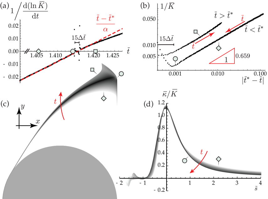
The points collapse onto a straight line, aside from a thin band of width $\approx 15\Delta\overline{t}$ where the large curvature is not well resolved by the discretization. A linear fit in figure 8a yields both the snapping time $\overline{t}^{*}$ (where the fitting line crosses the $t$-axis) and the exponent $\alpha$ (the reciprocal of the slope). This fit yields a value of the exponent $\alpha=0.659$ which is numerically close to 2/3 (we do not know whether this is a coincidence) and $\overline{t}^{*}=1.415$. The latter is close to (but less than) the singular time $2t_{\mathrm{LO}}\sqrt{a/L}=2\sqrt{2/3}\approx 1.63$ found by extrapolating the asymptotic behavior in the immediate aftermath after lift-off, see equation (19). These numerical values of $\overline{t}^{*}$ and $\alpha$ have been obtained in the particular case $\pi_{2}=1/(2\pi)$ and $\pi_{3}=0$. We suspect, however, that the exponent $\alpha$ can be explained by a boundary-layer theory and that it is actually independent on $\pi_{2}$ and $\pi_{3}$. Unfortunately, we can offer no proof for this statement.

As observed in the experiments (see §2), the string remains straight in the simulations along an interval of length $\ell(t)$ comprising the free end, at all times until $t^{*}$. This straight portion of the string is apparent in figures 7a and 8c. It defines the region denoted by (I), which is adjacent to the region (II) of large curvature (see Fig 2c). The dimensionless length $\overline{\ell}=\ell/L$ is found numerically to scale like $\overline{\ell}\sim(\overline{t}^{*}-\overline{t})^{\beta}$, with $\beta=1.08\pm 0.2$ (fit not shown). The numerical accuracy on this exponent $\beta$ is not as good as that of $\alpha$ as the determination of the straight region is sensitive to numerical noise. It is clear from our numerical data, however, that the exponent $\beta$ is larger than $\alpha$, meaning that the length of the straight region near the free end vanishes more quickly than the minimum radius of curvature as $\overline{t}\to\overline{t}^{*}$, $\overline{t}<\overline{t}^{*}$.

Next, we proceed to use our analysis to uncover a self-similar behavior in the curvature profile. Anticipating that the point of maximal curvature plays a central role we introduce a weighing to capture its position:

$$\langle\overline{s}\rangle({\overline{t}})=\frac{\int_{0}^{1}\overline{s}\,\overline{\kappa}^{p}(\overline{s},\overline{t})\,\mathrm{d}\overline{s}}{\int_{0}^{1}\overline{\kappa}^{p}(\overline{s},\overline{t})\,\mathrm{d}\overline{s}}\textrm{.}$$ (28)

By design, the weighting is concentrated in the region of large curvature: $\langle\overline{s}\rangle({\overline{t}})$ yields the typical value of $\overline{s}$ at time $\overline{t}$ in the region (II) where the curvature diverges.

Finally we rescale the arc-length parameter to

$$\tilde{s}=\frac{\overline{s}-\langle\overline{s}\rangle({\overline{t}})}{1/\overline{K}(\overline{t})}\textrm{,}$$ (29)

By design, $\tilde{s}=0$ lies in the centre of the region with high curvature. In this definition, the offset $\langle\overline{s}\rangle({\overline{t}})$ allows us to ignore the straight region entirely (which shrinks according to a different exponent). We consider a set of simulation snapshots such that $1.405\leq\overline{t}\leq 1.414$, i.e. such that $0.001\leq\overline{t}^{*}-\overline{t}\leq 0.01$. This corresponds to the configurations bounded by the symbols ( ) and ( ) in figure 8b-c, with darker plots corresponding to times closer to the snapping time $\overline{t}^{*}$.

In figure 8d, we plot the rescaled curvature $\overline{\kappa}(s,t)/\overline{K}(t)$ as a function of the rescaled arc-length $\tilde{s}$ and obtain a good collapse. Note that the unscaled maximum curvature $\overline{K}$ varies by a factor $\sim 5$, from approximately 65 to 308, between the first and last snapshot in this series. Therefore, the collapse shows that the curvature distribution is self-similar close to the snapping time $\overline{t}^{*}$: consistently with our initial scaling assumption, the curvature scales like $\overline{\kappa}\sim(\overline{t}^{*}-\overline{t})^{-\alpha}$ in a region of size $\overline{s}-\langle\overline{s}\rangle\sim(\overline{t}^{*}-\overline{t})^{\alpha}$. Note that this analysis focuses on the behavior of the chain prior to snapping, so that $\overline{t}<\overline{t}^{*}$.

In summary, our analysis shows that the snapping singularity may characterized by a self-similar solution, whose scaling behaviours have been identified numerically.

7 Conclusions

In this paper, we have considered a degenerate version of Atwood’s machine, in which a single mass pulls a chain around a pulley. In stark contrast with the apparent simplicity of the setup we have found that the dynamics is extremely rich, successively displaying a ballooning instability of the chain and a snapping motion of its free end, reminiscent of what is seen in a cracking whip. We have shown that the chain dynamics is well captured by a frictionless string model and that some of its features may be captured by simple arguments. In particular we have shown that the geometry of the problem, through the imposed rotation of the chain around the pulley, is key to understanding how the end of the chain is able to ’beat’ the free-fall that drives its motion.

Our observations can be used to speculate on the peculiar hunting techniques of a variety of amphibians. Indeed, instead of throwing their tongue in a straight motion (as observed in chameleons [19, 20]), certain species of toads [21] and salamanders [22] adopt an unfurling tongue strategy. Of course, the reasons for such a mechanism are many and varied but we believe that the increase of tip velocity observed in the case of a chain is likely to reappear in problems involving a finite bending stiffness. It is then natural to wonder whether this geometrical amplification of acceleration may be used by these amphibians to allow them to maximize their chances of capturing a prey?

Finally, we note that while we have been able to rationalize some of the observations from experiment and simulation, others remain elusive. For example, predicting the shape of the ballooning region either with simple arguments, or preferably analytically, remains beyond our reach. Difficulties in doing so arise from the fact that the ‘base solution’ of the problem is unsteady (since $a>0$). An interesting avenue of research would be to explore the case where the chain is pulled at constant speed thus without any acceleration, potentially allowing for analytical developments. Similarly, there is hope that the self-similar exponent $\alpha$ and $\beta$ identified in the previous section can be explained by some boundary layer theory in future work.

Appendix A The effect of gravity immediately after lift-off

For simplicity, the main portion of the paper focusses on the problem in the absence of gravity. In this Appendix, we show how the results derived in §55.1 for the behaviour immediately following lift-off are altered once gravity is included. These results confirm that, in this case at least, gravity affects the results quantitatively, rather than qualitatively.

A.1 The unknown chain acceleration

Immediately after lift-off, the free end of the chain accelerates at an unknown rate $\dot{v}_{\mathrm{hang}}$. To determine this acceleration, we repeat the argument of § 55.1 incorporating gravity: the normal force arising from the tension at the material position that was at C when lift-off started ($\rho_{\ell}(\dot{v}_{\mathrm{hang}}+g)s_{C}^{\mathrm{LO}}\kappa$) is equated with the force arising from the centripetal acceleration ($\rho_{\ell}v_{\mathrm{hang}}^{2}\kappa$) for some undetermined curvature $\kappa$. We then have that (18) becomes

$$(\dot{v}_{\mathrm{hang}}+g)s_{C}^{\mathrm{LO}}=v_{\mathrm{hang}}^{2},$$ (30)

which can be solved with initial condition $v_{\mathrm{hang}}(t_{\mathrm{LO}})=at_{\mathrm{LO}}$ to give

$$v_{\mathrm{hang}}=\sqrt{gs_{C}^{\mathrm{LO}}}\coth\left[\alpha-\sqrt{\frac{g}{s_{C}^{\mathrm{LO}}}}(t-t_{\mathrm{LO}})\right],$$ (31)

where

$$\coth\alpha=\frac{at_{\mathrm{LO}}}{\sqrt{gs_{C}^{\mathrm{LO}}}}.$$ (32)

The form of (31) appears to be substantially different to that in the absence of gravity, (19). However, the qualitative behaviour is, in fact very similar: $v_{\mathrm{hang}}(t)$ is an increasing function of $t>t_{\mathrm{LO}}$ and has a singularity at

$$t=t_{\mathrm{LO}}+\sqrt{\frac{s_{C}^{\mathrm{LO}}}{g}}\alpha.$$ (33)

Furthermore, a Taylor expansion of (31) reveals that

$$v_{\mathrm{hang}}=at+\frac{a^{2}t_{\mathrm{LO}}}{s_{C}^{\mathrm{LO}}}(t-t_{\mathrm{LO}})^{2}+O(t-t_{\mathrm{LO}})^{3},$$ (34)

so that the change in the pulling velocity occurs at $O(t-t_{\mathrm{LO}})^{2}$, as in the case without gravity (see figure 4a).

A.2 The excess length $\Delta L$

From the expression (31) for the acceleration of the hanging portion of the chain, we find that the excess length absorbed by the lifted off portion is

$$\Delta L =-s_{C}^{\mathrm{LO}}\log\frac{\sinh\left[\alpha-\sqrt{\frac{g}{s_{C}^{\mathrm{LO}}}}(t-t_{\mathrm{LO}})\right]}{\sinh\alpha}+\frac{a}{2}(t_{\mathrm{LO}}^{2}-t^{2})$$

$$=\left(a+\tfrac{g}{3}\right)\frac{(t-t_{\mathrm{LO}})^{3}}{3t_{\mathrm{LO}}}+O[(t-t_{\mathrm{LO}})^{4}].$$ (35)

This cubic growth of the excess length with time following lift-off echoes that found in the absence of gravity, given by (23). As already seen, the only significant difference is in the prefactor.

References

- [1] A. Goriely and T. McMillen. Shape of a cracking whip. Phys. Rev. Lett., 88(24):244301, 2002.
- [2] T. McMillen and A. Goriely. Whip waves. Physica D, 184(1):192–225, 2003.
- [3] S. Neukirch. Extracting DNA Twist Rigidity from Experimental Supercoiling Data. Phys. Rev. Lett., 93(19):198107, November 2004.
- [4] L. Carter. Submarine cables and the oceans: connecting the world. Number 31. UNEP/Earthprint, 2009.
- [5] P.-T. Brun, N. Ribe, and B. Audoly. An introduction to the mechanics of the lasso. Proc. R. Soc. A, 470(2171):20140512, 2014.
- [6] M. Habibi, N. M. Ribe, and D. Bonn. Coiling of elastic ropes. Phys. Rev. Lett., 99(15):154302, 2007.
- [7] B. Audoly and Y. Pomeau. Elasticity and geometry: from hair curls to the non-linear response of shells. Oxford University Press, 2010.
- [8] T. J. Healey and J. N. Papadopoulos. Steady axial motion of strings. J. Appl. Mech., 57:785–787, 1990.
- [9] J. A. Hanna and C. D. Santangelo. Slack dynamics on an unfurling string. Phys. Rev. Lett., 109(13):134301, 2012.
- [10] J. S. Biggins and M. Warner. Understanding the chain fountain. Proc. R. Soc. A, 470(2163):20130689, 2014.
- [11] J. S. Biggins. Growth and shape of a chain fountain. EPL, 106(4):44001, 2014.
- [12] M. Bergou, M. Wardetzky, S. Robinson, B. Audoly, and E. Grinspun. Discrete elastic rods. In ACM Transactions on Graphics (TOG), volume 27, page 63. ACM, 2008.
- [13] M. K. Jawed, F. Da, J. Joo, E. Grinspun, and P. M. Reis. Coiling of elastic rods on rigid substrates. Proc. Natl Acad. Sci., 111(41):14663–14668, October 2014.
- [14] B. Audoly, N. Clauvelin, P.-T. Brun, M. Bergou, E. Grinspun, and M. Wardetzky. A discrete geometric approach for simulating the dynamics of thin viscous threads. J. Comp. Phys., 253(C):18–49, November 2013.
- [15] J. A. Hanna. Jump conditions for strings and sheets from an action principle. Int. J. Solid Struct., 62:239–247, 2015.
- [16] M. Schagerl, A. Steindl, W. Steiner, and H. Troger. On the paradox of the free falling folded chain. Acta Mech., 125(1-4):155–168, 1997.
- [17] W. Tomaszewski and P. Pieranski. Dynamics of ropes and chains: I. the fall of the folded chain. New J. Phys., 7(1):45, 2005.
- [18] W. Tomaszewski, P. Pieranski, and J.-C. Geminard. The motion of a freely falling chain tip. Am. J. Phys., 74(9):776–783, 2006.
- [19] C. V. Anderson and S. M. Deban. Ballistic tongue projection in chameleons maintains high performance at low temperature. Proc. Natl Acad. Sci., 107(12):5495–5499, 2010.
- [20] D. E. Moulton, T. Lessinnes, S. O’Keeffe, L. Dorfmann, and A. Goriely. The elastic secrets of the chameleon tongue. Proc. R. Soc. A, 472(2188):20160030, 2016.
- [21] S. M. Deban and A. K. Lappin. Thermal effects on the dynamics and motor control of ballistic prey capture in toads: maintaining high performance at low temperature. J. Exp. Bio., 214(8):1333–1346, 2011.
- [22] S. M. Deban, J. C. O’Reilly, U. Dicke, and J. L. van Leeuwen. Extremely high-power tongue projection in plethodontid salamanders. J. Exp. Bio., 210(4):655–667, 2007.