Quasi-matter bounce and inflation in the light of the CSL model

Abstract

The Continuous Spontaneous Localization (CSL) model has been proposed as a possible solution to the quantum measurement problem by modifying the Schrödinger equation. In this work, we apply the CSL model to two cosmological models of the early Universe: the matter bounce scenario and slow roll inflation. In particular, we focus on the generation of the classical primordial inhomogeneities and anisotropies that arise from the dynamical evolution, provided by the CSL mechanism, of the quantum state associated to the quantum fields. In each case, we obtained a prediction for the shape and the parameters characterizing the primordial spectra (scalar and tensor), i.e. the amplitude, the spectral index and the tensor-to-scalar ratio. We found that there exist CSL parameter values, allowed by other non-cosmological experiments, for which our predictions for the angular power spectrum of the CMB temperature anisotropy are consistent with the best fit canonical model to the latest data released by the Planck Collaboration.

I Introduction

After approximately three decades since the cosmological inflationary paradigm was conceived Guth (1981); Starobinsky (1980); Linde (1982); Albrecht and Steinhardt (1982), all of its generic predictions have withstood the confrontation with observational data, in particular, those coming from the Cosmic Microwave Background (CMB) radiation Ade et al. (2015a, b, c). That has led a large group of cosmologists to consider inflation as a well established theory of the early Universe. Inflation was originally proposed to provide a solution to the puzzles of the hot Big Bang theory (e.g. the horizon and flatness problems). However, the modern success of inflation is that, allegedly, it can offer us an explanation about the origin of the primordial inhomogeneities Mukhanov and Chibisov (1981); Starobinsky (1983); Hawking and Moss (1983); Bardeen et al. (1983). The standard argument is also rather pictorial: the quantum fluctuations of the vacuum associated to the inflaton are stretched out to cosmological scales due to the accelerated expansion of the spacetime; those fluctuations are considered the seeds of all large scale structures observed in the Universe. Furthermore, in Ref. Martin and Vennin (2016) is investigated the detectability of possible traces of the quantum nature regarding the primordial perturbations.

On the other hand, proponents of alternative scenarios to inflation argue that even if it is the most fashionable model of the early Universe, that does not mean it is necessarily true Ijjas et al. (2013); Battefeld and Peter (2015). Furthermore, another feature that would make alternative models worthwhile of study is that they might avoid some long standing puzzles of the inflationary paradigm. Among those issues, we can mention: the subject of eternal inflation, a feature that is present in almost every model of inflation Vilenkin (1983) and which also leads to the controversial topic of the multiverse; the initial singularity problem and the trans-Planckian problem for primordial perturbations Martin and Brandenberger (2001), which are related by the fact that one is interpolating the solutions provided by General Relativity in regimes where it may no longer be valid; and finally, it has been argued that the potentials associated to the inflaton, that best fit the latest observed data, need to be fine-tuned Ijjas et al. (2014); Ijjas and Steinhardt (2016). Although the aforementioned problems are not considered real problems by some scientists Linde (2015); Guth et al. (2014), others seem to disagree Brandenberger (2011); Ijjas and Steinhardt (2016). However, we think that if other alternative models can reproduce the main results linked to inflation, we should make use of the observational data available to test them.

One of the alternative models to inflation that seems to be consistent with the latest data is the so called matter bounce scenario (MBS) Brandenberger (2011); Elizalde et al. (2015); de Haro and Cai (2015); de Haro and Amorós (2015); Haro (2013); Haro and Amoros (2014); Cai (2014); Cai et al. (2016). In this cosmological model, the initial singularity of the standard model is replaced by a non-singular bounce. That is, instead of an ever-expanding Universe, it assumes an early contracting matter-dominated Universe, which continues to evolve towards a bouncing phase and, later, enters into the expanding-phase of standard cosmology. The Universe described by the MBS relies on a single scalar field satisfying an equation of state that mimics that of a dust-like fluid. Additionally, in order to describe successfully a bouncing phase with a single scalar field, one needs to use cosmologies beyond the realm of General Relativity, such as, loop quantum cosmologies, teleparallel $F(T)$ gravity or $F(R)$ gravity. Proponents of the MBS claim that the potential associated to the scalar field is less fine-tuned than that of inflation, and also solves the historical problem of requiring very special initial conditions for the Big Bang model Elizalde et al. (2015); de Haro and Cai (2015), which originally motivated the development of the inflationary framework. However, the MBS is not exactly problem free. A complete assessment of the present conceptual issues is provided in Ref. de Haro and Cai (2015). In spite of not being completely finished from a theoretical point of view, the MBS is quite simple in its treatment of the primordial perturbations. That makes it an interesting case of study for the purpose of this article. In particular, the generation of the primordial perturbations is depicted during the contracting phase, i.e. in a regime where gravity is well described by General Relativity, and the perturbations correspond to inhomogeneities of a single scalar field.

In addition to the prior puzzles and successes of inflation and the MBS, there remains an important question: what is the precise physical mechanism that converts quantum fluctuations of the vacuum into classical perturbations of the spacetime? This question has been the subject of numerous works in the past and the consensus seems to favor the decoherence framework Kiefer and Polarski (2009); Halliwell (1989); Kiefer (2000); Polarski and Starobinsky (1996); Grishchuk and Sidorov (1990). Nevertheless, decoherence cannot address that question by itself. In other words, even if one would choose (or not) to embrace the decoherence program, a particular interpretation of Quantum Mechanics must be selected (implicitly or explicitly). The Copenhagen–orthodox–interpretation requires to identify a notion of observer that performs a measurement on the system; which, in the decoherence framework, is equivalent to identify the unobservables or external degrees of freedom of the system. It is not clear how to do such identifications if the system is the early Universe. Other interpretations such as many-worlds, consistent histories and hidden variables formulations, might be adopted with varying degrees of success (see for instance Pinto-Neto et al. (2012); Valentini (2010); Goldstein et al. (2015)).

In the present article, in order to address the quantum-to-classical transition of the primordial perturbations, we will choose to work with the Continuous Spontaneous Localization (CSL) model. The CSL model belongs to a large class of models known as objective dynamical reduction models or simply called collapse models. Collapse models attempt to provide a solution to the measurement problem of Quantum Mechanics Ghirardi et al. (1986); Pearle (1989); Bassi and Ghirardi (2003); Bassi et al. (2013, 2012). The proponents of these models state that the measurement problem originates from the linear character of the quantum dynamics encoded in the Schrödinger equation. The common idea shared in these collapse models is to introduce some nonlinear stochastic corrections to the Schrödinger equation that breaks its linearity. According to the collapse models, a noise field couples nonlinearly with the system (usually with the spatial degree of freedom of the system), inducing a spontaneous random localization of the wave function in a sufficiently small region of the space. Suitably chosen collapse parameters make sure that micro-systems evolve essentially (but not exactly) following the dynamics provided by the Schrödinger equation, while macro-systems are extremely sensible to the nonlinear effects resulting in a perfectly localization of the wave function. Furthermore, there is no need to mention or to introduce a notion of an observer/measurement device as in the Copenhagen interpretation, which is a desired feature in the context of the early Universe and cosmology in general.

The CSL model has been applied before to the inflationary Universe in an attempt to explain the quantum-to-classical transition of the primordial perturbations Martin et al. (2012); Cañate et al. (2013); Das et al. (2013, 2014); León and Bengochea (2016). Also, recently a new effective collapse mechanism, independent of the CSL model, has been proposed to deal with the measurement problem during the inflationary era Alexander et al. (2016). However, among those works, the key role played by the collapse mechanism varies and also yields different predictions for the primordial power spectrum, some of which might be consistent with the observational data. In the present article, we will subscribe to the conceptual point of view first presented in Perez et al. (2006); Cañate et al. (2013), which was developed within the semiclassical gravity framework, and latter in Diez-Tejedor et al. (2012); León and Bengochea (2016) was extended to the standard quantization procedure of the primordial perturbations using the so called Mukhanov-Sasaki variable Mukhanov and Chibisov (1981); Kodama and Sasaki (1984). The main role that we advocate for the dynamical reduction mechanism of the state vector, modeled in this paper by the CSL model, is to directly generate the primordial curvature perturbations. Specifically, the initial state of the quantum field–the vacuum state–evolves dynamically according to the modified Schrödinger equation provided by the CSL model. This evolution leads to a final state that does not share the initial symmetry of the vacuum, i.e. it is not homogeneous and isotropic. In this way, the collapse mechanism generates the inhomogeneities and anisotropies of the matter fields. These asymmetries are codified in the evolved quantum state and, thus, are responsible for generating the perturbations of the spacetime.

Note that the previous prescription, regarding our approach to address the birth of the primordial perturbations, does not require the inclusion of an exponential expansion phase in the Universe that “stretches out” the quantum fluctuations of the vacuum (or the squeezing of the field variables as usually argued). Therefore, in principle, it should be possible to extend our picture to alternative scenarios dealing with the origin of the cosmological perturbations. Moreover, since the cosmic observations are well constrained, it should also be feasible to test the predictions that result from applying our framework in those alternative cosmological models. In the present article, we focus on the implementation of the CSL model within the framework of the MBS and, in parallel, we present the same appliance of the CSL model to the slow roll inflationary model of the early Universe. In this way, we can appreciate more clearly where the CSL model enters into the picture; particularly at the moment when computing the theoretical predictions. The main motivation behind the present work is that if the CSL model can be truly considered as a physical model of the quantum world, which also avoids the standard quantum measurement problem, then it should also be possible to use it in different contexts from the traditional laboratory settings. The cosmological context provides a rich avenue to explore such foundational issues and, more important, there exist sufficient precise data to test the initial hypotheses. As a consequence, we will analyze the predictions resulting from implementing the CSL model in the MBS and in the inflationary model of the early Universe, and we will compare the corresponding results with the one provided by the best fit standard cosmological model. Additionally, we will focus on the range of values allowed for the parameters of the CSL model, experimentally tested Toros and Bassi (2016a); Toros and Bassi (2016b) in non-cosmological frameworks.

The paper is organized as follows: in Sect. II, we provide a very brief synopsis of the main features of the CSL model, with particular emphasis on those that will be useful for the next sections. In Sect. III, we present the characterization of the primordial perturbations within the two cosmological models that we are considering, i.e. the MBS and standard slow roll inflation. In Sect. IV, we show the connection between the observational quantities and the theoretical predictions that result from adopting our conceptual point of view concerning the CSL model. In Sect. V, we explicitly show the implementation of the CSL model to the MBS and inflation, and we also present the predictions for the primordial power spectra (scalar and tensor) in each case. In Sect. VI, we discuss the implications of the results obtained; additionally, we compare the predicted scalar power spectra with the standard one. In Sect. VII, we analyze the viability of the CSL model using the data extracted from the CMB when considering the best fit cosmological model. Finally, in Sect. VIII, we end with our conclusions. We include an Appendix containing the computational details that led to the results presented in Sect. V.

II A concise synopsis of the CSL model

In this section, we provide a brief summary of the relevant features of the CSL model; for a detailed review, we refer the reader to Refs. Bassi and Ghirardi (2003); Bassi et al. (2013).

In the CSL model, the modification of the Schrödinger equation induces a collapse of the wave function towards one of the possible eigenstates of an operator $\hat{\varTheta}$, called the collapse operator, with certain rate $\lambda$. The self-induced collapse is due to the interaction of the system with a background noise $\mathcal{W}(t)$ that can be considered as a continuous-time stochastic process of the Wiener kind. The modified Schrödinger equation drives the time evolution of an initial state as

$$|\Psi,t\rangle=\hat{T}\exp\left\{-\int_{t_{0}}^{t}dt^{\prime}\left[i\hat{H}+\frac{1}{4\lambda}\left(\mathcal{W}(t^{\prime})-2\lambda\hat{\varTheta}\right)^{2}\right]\right\}|\Psi,t_{0}\rangle,$$ (1)

with $\hat{T}$ the time-ordering operator. The probability associated with a particular realization of $\mathcal{W}(t)$ is,

$$P[\mathcal{W}(t),t]D\mathcal{W}(t)=\langle\Psi,t|\Psi,t\rangle\prod_{t_{i}=t_{0}}^{t}\frac{d\mathcal{W}(t_{i})}{\sqrt{2\pi\lambda/dt}}.$$ (2)

The norm of the state $|\Psi,t\rangle$ evolves dynamically, and Eq. (2) implies that the most probable state will be the one with the largest norm. From Eqs. (1) and (2), it can be derived the evolution equation of the density matrix operator $\hat{\rho}$. That is,

$$\frac{d\hat{\rho}}{dt}=-i[\hat{H},\hat{\rho}]-\frac{\lambda}{2}[\hat{\varTheta},[\hat{\varTheta},\hat{\rho}]].$$ (3)

The density matrix operator can be used to obtain the ensemble average of the expectation value of an operator $\overline{\langle\hat{O}\rangle}=\textrm{Tr}[\hat{O}\hat{\rho}]$. Henceforth, from Eq. (3) it follows that

$$\frac{d}{dt}\overline{\langle\hat{O}\rangle}=-i\overline{\langle[\hat{O},\hat{H}]\rangle}-\frac{\lambda}{2}\overline{\langle[\hat{\varTheta},[\hat{\varTheta},\hat{O}]]\rangle}.$$ (4)

The average is over possible realizations of the noise $\mathcal{W}(t)$, each realization corresponding to a single outcome of the final state $|\Psi,t\rangle$.

One of the most important features of collapse models is the so-called amplification mechanism. That is, assuming that the reduction (collapse) rates for the $M$ constituents of a macroscopic object are equal ($\lambda^{i}=\lambda$), it can be proved that the reduction rate for the center of mass of an $M$-particle system is amplified by a factor of $M$ with respect to that of a single constituent Ghirardi et al. (1986, 1990); in other words, $\lambda_{\textrm{macro}}=M\lambda$.

The parameter $\lambda$ sets the strength of the collapse process. In the original model, proposed by Ghirardi-Rimmini-Webber (GRW), the authors suggested a value of $\lambda_{\textrm{GRW}}\simeq 10^{-16}$ s^-1 for $r_{C}\simeq 100$ nm. However, Adler suggested a greater value $\lambda_{\textrm{Adler}}\simeq 10^{-8}$ s^-1 for $r_{C}\simeq 100$ nm Adler (2007) (the parameter $r_{C}$ is called the correlation length of the noise and provides a measure for the spatial resolution of the collapse Ghirardi et al. (1986, 1990); Bassi and Ghirardi (2003)). Recent experiments have been devised to set bounds on the parameter $\lambda$ Bahrami et al. (2014); Vinante et al. (2015). Furthermore, it is claimed that matter-wave interferometry provides the most generic way to experimentally test the collapse models Toros and Bassi (2016a); Toros and Bassi (2016b). Those results suggest that the range between $\lambda_{\textrm{GRW}}$ and $\lambda_{\textrm{Adler}}$ is still viable for some variations of the original CSL model (e.g. by considering non-white noise).

Henceforth, the main characteristics of the CSL model are: (1) The modification to the Schrödinger equation is nonlinear and leads to a breakdown of the superposition principle for macroscopic objects; (2) The random nature of Quantum Mechanics is concealed in the noise $\mathcal{W}(t)$ and is consistent with Born’s rule; (3) An amplification mechanism exists, through the parameter $\lambda$ which is related to the strength of the collapse. This strength is weak for microscopic objects and strong for macroscopic bodies.

Another main aspect of the collapse models is that the collapse mechanism injects energy into the system. In fact, previous works have performed a preliminary analysis using cosmological data to set bounds on the value of $\lambda$ Lochan et al. (2012). The energy increase is minimal, e.g. for a particle of mass $m=10^{-23}$ g, one obtains $\delta E/t\simeq 10^{-25}$ eV s^-1 Bassi and Ghirardi (2003). In other words, an increase of $10^{-8}$ eV will take $10^{10}$ years. However, even if the energy increase can be ignored at the phenomenological level, a more realistic model should remove this issue.

Moreover, the increase of energy in the collapse models leads to difficulties when trying to formulate relativistic collapse models. Additionally, the collapse mechanism occurs in such a way that is nonlocal. This implies that the collapse of the wave function must be instantaneous or superluminal (but the nonlocal features cannot be exploited to send signals at superluminal speed). Also, the nonlocality is necessary to ensure that the models are consistent with the violation of Bell’s inequalities. Several relativistic models have been proposed so far Tumulka (2006); Bedingham et al. (2013); Pearle (2015), none of which can be considered completely finished. In spite of the lack of a relativistic collapse model, we will apply the CSL model to the primordial Universe, i.e. to inflation and the MBS, but in order to provide a more detailed picture, we need first to establish the mathematical framework of the primordial Universe in the two approaches considered in this work.

III Two approaches: accelerated expansion or quasi-matter contraction

This section presents the details of the two cosmological approaches, describing the dynamics of the Universe, that we will be considering in the rest of the manuscript. In particular, we are going to work with the following two scenarios:

1. An accelerated expansion of the early Universe given by the simplest inflationary model, that is, a single scalar field in the slow roll approximation with canonical kinetic term. Since such a model is probably very well known for most readers, we will not dwell into much detail here.

2. The MBS Elizalde et al. (2015); de Haro and Cai (2015); de Haro and Amorós (2015); Haro (2013); Haro and Amoros (2014), a cosmological model in which the Universe undertakes a quasi-matter contracting phase, then experiences a non-singular bounce and finally enters into the standard cosmological expansion. Since in this model the primordial perturbations are born during the contracting stage of the Universe, we will focus exclusively on that cosmic stage. We will refer to such a stage as the quasi-matter contracting Universe (QMCU).

III.1 The background

The inflationary Universe and the QMCU are both described by Einstein equations $G_{ab}=8\pi GT_{ab}$ ($c=1$), while the matter fields are characterized by a single scalar field. In the case of inflation the scalar field is the inflaton $\phi$, and in the QMCU the scalar field will be denoted by $\varphi$.

As mentioned earlier, for inflation, we will consider standard slow roll inflation. In that case, the background spacetime is described by a quasi-de Sitter Universe, characterized by $\mathcal{H}\simeq-1/[\eta(1-\epsilon)]$, with $\mathcal{H}\equiv a^{\prime}/a$ the conformal expansion rate, $a$ being the scale factor and the slow roll parameter is defined as $\epsilon\equiv 1-\mathcal{H}^{\prime}/\mathcal{H}^{2}$; a prime denotes partial derivative with respect to conformal time $\eta$. The energy density of the Universe is dominated by the potential of the inflaton $V$, and during slow roll inflation the condition $\epsilon\simeq M_{P}^{2}/2(\partial_{\phi}V/V)^{2}\ll 1$ is satisfied, with $M_{P}^{2}\equiv(8\pi G)^{-1}$ the reduced Planck mass. Since we will work in a full quasi-de Sitter expansion, another useful parameter to characterize slow roll inflation is the second slow roll parameter, i.e. $\delta\equiv\epsilon-\epsilon^{\prime}/2\mathcal{H}\epsilon\ll 1$.

In the case of the QMCU, the starting point is also a flat FLRW geometry that leads to the Friedmann and conservation equations. The field $\varphi$ is separated into an homogeneous part $\varphi_{0}(\eta)$ plus small inhomogeneities $\delta\varphi(\textbf{x},\eta)$. The homogeneous part satisfies

$$\mathcal{H}^{2}=\frac{a^{2}}{3M_{P}}\left(\frac{\varphi_{0}^{\prime 2}}{2a^{2}}+W\right);\quad\varphi_{0}^{\prime\prime}+2\mathcal{H}\varphi_{0}^{\prime}+a^{2}\partial_{\varphi}W=0,$$ (5)

where $W$ is the potential associated to the field $\varphi$.

In the QMCU, it is assumed that the equation of state associated to the scalar field almost mimics that of ordinary matter, i.e. $P=\omega\rho$ such that $|\omega|\ll 1$; the latter implies $\varphi_{0}^{\prime 2}\simeq 2a^{2}W$. Consequently, the scale factor (in conformal time) evolves as $a(\eta)\simeq\eta^{2}/9$.

The quasi-matter contraction is characterized with a small parameter $|\overline{\epsilon}|\ll 1$, which plays the same role as the slow roll parameter in inflation. The parameter $\overline{\epsilon}$ is defined as (see e.g. Elizalde et al. (2015))

$$\overline{\epsilon}\equiv-\frac{2}{3}\left(\frac{1}{2}+\frac{\mathcal{H}^{\prime}}{\mathcal{H}^{2}}\right)\simeq\frac{1}{3}\left(\frac{\partial_{\varphi}W}{W}\right)^{2}-1.$$ (6)

The case $\overline{\epsilon}=0$ corresponds to an exact matter-dominated contracting phase (note that $\overline{\epsilon}=\omega$). Furthermore, for sake of completeness we introduce another parameter

$$\overline{\delta^{2}}\equiv\frac{\overline{\epsilon}^{\prime}}{2\mathcal{H}}\simeq-\partial_{\varphi}\left(\frac{\partial_{\varphi}W}{W}\right),$$ (7)

such that $|\overline{\delta^{2}}|\ll|\overline{\epsilon}|$. The parameter $|\overline{\delta^{2}}|$ is analog to the $\delta$ parameter of slow roll inflation and it is related to the running of the spectral index in the QMCU model (see e.g. Elizalde et al. (2015)).

As is well known, it is not straightforward to accomplish a non-singular bounce within the framework of General Relativity by considering a single canonical scalar field, since the null energy condition (NEC) is violated (see for instance Battefeld and Peter (2015); de Haro and Cai (2015)). As a consequence, one possible option is to work with cosmologies within the context of modified gravity theories. In the case of the QMCU presented in Elizalde et al. (2015); de Haro and Cai (2015), the authors worked within the framework of holonomy corrected loop quantum cosmology and teleparallel $F(T)$ gravity.

It is also important to note that even if a non-singular bounce cannot be achieved within General Relativity, the origin of the primordial perturbations is assumed to take place during the contracting (pre-bounce) phase of the Universe, where the curvature and energy scales are low enough to be described by General Relativity. On the other hand, one must present the conditions that need to be fulfilled such that the shape of the primordial spectrum, associated to the perturbations, remains practically unchanged when passing through the bounce. We will discuss this subject in more detail in the next section.

III.2 Perturbations

In the inflationary Universe and in the QMCU, one can separate the scalar field into an homogeneous part plus small inhomogeneous perturbations. Moreover, the metric associated to the spacetime, in both cases, is described by a FLRW background metric plus perturbations; which are classified as scalar, vector and tensor types (in this paper we will not consider vector perturbations). One useful quantity to describe the scalar (an also the tensor) perturbations is the so called Mukhanov-Sasaki (MS) variable. During inflation, the MS variable is defined by

$$v(\textbf{x},\eta)\equiv a(\eta)\left[\delta\phi(\textbf{x},\eta)+\frac{\phi_{0}^{\prime}(\eta)}{\mathcal{H}(\eta)}\Phi(\textbf{x},\eta)\right],$$ (8)

with $\Phi$ the gauge invariant quantity known as the Bardeen potential Bardeen (1980), which, in the longitudinal gauge, corresponds to the curvature perturbation. A similar expression to Eq. (8) can be used in the QMCU by replacing the fields $\phi_{0}^{\prime}$ and $\delta\phi$ with $\varphi_{0}^{\prime}$ and $\delta\varphi$, respectively. The advantage of relying on the MS variable is that, when expanding the action of a scalar field minimally coupled to gravity into second order scalar perturbations, one obtains $\delta^{(2)}S=\frac{1}{2}\int d\eta d^{3}\textbf{k}\mathcal{L}$, where

$$\mathcal{L}=v_{\textbf{k}}^{\prime}v_{\textbf{k}}^{\star^{\prime}}-k^{2}v_{\textbf{k}}v_{\textbf{k}}^{\star}-\frac{z^{\prime}}{z}\left(v_{\textbf{k}}v_{\textbf{k}}^{\star^{\prime}}+v_{\textbf{k}}^{\prime}v_{\textbf{k}}^{\star}\right)+\left(\frac{z^{\prime}}{z}\right)^{2}v_{\textbf{k}}v_{\textbf{k}}^{\star},$$ (9)

with $v_{\textbf{k}}$ the Fourier modes associated to the MS variable, $z=a\phi_{0}^{\prime}/\mathcal{H}$ during inflation, and $z=a\varphi_{0}^{\prime}/\mathcal{H}$ when considering the QMCU. However, it is important to note that during the bouncing phase, the action given by the Lagrangian in Eq. (9) remains the same but the expression for $z$ changes (see Ref. Haro (2013) for an explicit calculation within $F(T)$ theories). On the other hand, during the contraction phase, the quantity $z^{\prime}/z$ can be written explicitly in terms of the QMCU parameter $\bar{\epsilon}$, as in a similar fashion using the slow roll inflation parameters, i.e.

$$\frac{z^{\prime}(\eta)}{z(\eta)}=\frac{\beta}{\eta};\qquad\textrm{where}\qquad\beta\equiv\begin{cases}-(1+2\epsilon-\delta)\>\>\textrm{if assuming the inflationary universe }\\ 2(1-3\bar{\epsilon})\>\>\textrm{if assuming the QMCU }\\ \end{cases}$$ (10)

Note that, since $|\overline{\delta^{2}}|\ll|\overline{\epsilon}|$, the $\overline{\delta^{2}}$ parameter does not enter into the expression $z^{\prime}/z$ at first order for the QMCU.

The CSL model is based on a nonlinear modification to the Schrödinger equation; consequently, it will be advantageous to perform the quantization of the perturbations in the Schrödinger picture, where the relevant physical objects are the Hamiltonian and the wave functional. The Hamiltonian associated to $\mathcal{L}$ in Eq. (9) is $H=\frac{1}{2}\int d^{3}\textbf{k}\>(H_{\textbf{k}}^{R}+H_{\textbf{k}}^{I})$, with

$$H^{R,I}_{\textbf{k}}=p_{\textbf{k}}^{R,I}p_{\textbf{k}}^{R,I}+\frac{z^{\prime}}{z}\left(v_{\textbf{k}}^{R,I}p_{\textbf{k}}^{R,I}+v_{\textbf{k}}^{R,I}p_{\textbf{k}}^{R,I}\right)+k^{2}v_{\textbf{k}}^{R,I}v_{\textbf{k}}^{R,I},$$ (11)

where the indexes $R,I$ denote the real and imaginary parts of $v_{\textbf{k}}$ and $p_{\textbf{k}}$. The canonical conjugated momentum associated to $v_{\textbf{k}}$ is $p_{\textbf{k}}=\partial\mathcal{L}/\partial v_{\textbf{k}}^{\star^{\prime}}$, i.e.

$$p_{\textbf{k}}=v_{\textbf{k}}^{\prime}-\frac{z^{\prime}}{z}v_{\textbf{k}}.$$ (12)

Since $v(\textbf{x},\eta)$ is a real field, $v_{\textbf{k}}^{\star}=v_{-\textbf{k}}$.

We promote $v_{\textbf{k}}$ and $p_{\textbf{k}}$ to quantum operators, by imposing canonical commutations relations $[\hat{v}_{\textbf{k}}^{R,I},\hat{p}_{\textbf{k}^{\prime}}^{R,I}]=i\delta(\textbf{k}-\textbf{k}^{\prime})$.

In the Schrödinger picture, the wave functional $\Psi[v(\textbf{x},\eta)]$ characterizes the state of the system. Furthermore, in Fourier space, the wave functional can be factorized into modes components $\Psi[v(\textbf{x},\eta)]=\Pi_{\textbf{k}}\Psi_{\textbf{k}}^{R}(v_{\textbf{k}}^{R})\Psi_{\textbf{k}}^{I}(v_{\textbf{k}}^{I})$. From now on, we will deal with each mode separately. Henceforth, each mode of the wave functional, associated to the real and imaginary parts of the canonical variables, satisfies the Schrödinger equation $\hat{H}_{\textbf{k}}^{R,I}\Psi_{\textbf{k}}^{R,I}=i\partial\Psi_{\textbf{k}}^{R,I}/\partial\eta$, with the Hamiltonian provided by (11). Note that one can also choose to work with the wave functional in the momentum representation, i.e. $\Psi[p(\textbf{x},\eta)]=\Pi_{\textbf{k}}\Psi_{\textbf{k}}^{R}(p_{\textbf{k}}^{R})\Psi_{\textbf{k}}^{I}(p_{\textbf{k}}^{I})$.

The standard assumption is that, at an early conformal time $\tau\to-\infty$, the modes are in their adiabatic ground state, which is a Gaussian centered at zero with certain spread. This applies to both, the inflationary Universe and the QMCU. In addition, this ground state is commonly referred to as the Bunch-Davies vacuum. Thus, the conformal time $\eta$ is in the range $[\tau,0^{-})$.

Given that the initial quantum state is Gaussian, its shape will be preserved during its evolution. The explicit expression of the Gaussian state, in the field representation, is:

$$\Psi^{R,I}(\eta,v_{\textbf{k}}^{R,I})=\exp\left[-A_{k}(\eta)(v_{\textbf{k}}^{R,I})^{2}+B_{k}(\eta)v_{\textbf{k}}^{R,I}+C_{k}(\eta)\right],$$ (13)

and, equivalently, in the momentum representation

$$\Psi^{R,I}(\eta,p_{\textbf{k}}^{R,I})=\exp\left[-\tilde{A}_{k}(\eta)(p_{\textbf{k}}^{R,I})^{2}+\tilde{B}_{k}(\eta)p_{\textbf{k}}^{R,I}+\tilde{C}_{k}(\eta)\right].$$ (14)

Therefore, the wave functional evolves according to Schrödinger equation, with initial conditions given by $A_{k}(\tau)=k/2,{\tilde{A}}_{k}(\tau)=1/2k,B_{k}(\tau)={\tilde{B}}_{k}(\tau)=C_{k}(\tau)={\tilde{C}}_{k}(\tau)=0$ corresponding to the Bunch-Davies vacuum, which is perfectly homogeneous and isotropic in the sense of a vacuum state in quantum field theory. The fact that we are introducing the wave functional in the field and momentum representations is related to the choice of the collapse operator in the CSL model, i.e., since there is no physical reason to choose one over the other, both choices are equally acceptable (at least from the phenomenological point of view). In the next section, we will show how to extract the physical quantities from the theory to be compared with the observations.

IV Theoretical predictions and observational quantities

We begin this section by making some key remarks about the conceptual aspects of our approach and, then, we proceed to identify the relevant physical quantities that will be related with the observed data. We encourage the reader to consult Refs. Perez et al. (2006); Sudarsky (2011); Landau et al. (2013) for a complete discussion regarding our full picture of the role played by the dynamical reduction of wave function in the cosmological setting. As a matter of fact, the relation between the observables and the predictions from the theory, using the Mukhanov-Sasaki variable during inflation and the CSL model, has been previously exposed in León and Bengochea (2016); however, in this section we reproduce the key arguments of such a reference to make the present paper as self-contained as possible. Thus, there is no original work in the following of this section.

The main role for invoking the collapse of the wave function is to find a physical mechanism for breaking the initial homogeneity and isotropy associated to both, the quantum state and the spacetime. More specifically, we assume that a nonlinear modification to the Schrödinger equation, which in the present work is provided by the CSL model, can break the homogeneity and isotropy associated to the vacuum state and, in turn, it can generate the metric perturbations, which correspond to the primordial curvature perturbation.

Note that in the literature one can found statements suggesting that the vacuum fluctuations somehow become classical when the proper wavelength associated to the perturbations becomes larger than the Hubble radius Kiefer and Polarski (2009); Riotto (2002). Nevertheless, there is nothing in the dynamics governed by the traditional Schrödinger equation that can change the symmetry of the vacuum state, the symmetry being the homogeneity and isotropy. As a consequence, if the quantum state is perfectly symmetric and the Quantum Theory teaches us that the symmetries of a physical system must be encoded in the quantum state, then there is no clear way to describe the inhomogeneities and anisotropies of the spacetime in the quantum sense. If the quantum state of the system is perfectly symmetric, then its classical description must also be exactly symmetric. Thus, there is a lack of a proper explanation concerning the emergence of the primordial inhomogeneities and anisotropies in the Universe. That is why some non-standard interpretations of Quantum Mechanics, that make use of the Schrödinger equation (e.g. many-worlds, consistent histories, etc.), cannot provide a satisfactory answer to the problem at hand. It is important to note that the previous discussion applies to both cosmological models, the QMCU and inflation.

The modified Schrödinger equation given by the CSL model can successfully change the symmetries of the vacuum state and, at the same time, be responsible for the birth of the primordial curvature perturbation.

Specifically, in the comoving gauge, the curvature perturbation $\mathcal{R}(\textbf{x},\eta)$ and the MS variable $v(\textbf{x},\eta)$ are related by $\mathcal{R}(\textbf{x},\eta)=v(\textbf{x},\eta)/z(\eta)$. Thus, a quantization of $v(\textbf{x},\eta)$ implies a quantization of $\mathcal{R}(\textbf{x},\eta)$. The question that arises now is: how to relate the quantum objects $\hat{v}(\textbf{x},\eta)$ and $\hat{\mathcal{R}}(\textbf{x},\eta)$? Furthermore, one may wonder how to relate the physical observables, such as the temperature anisotropies of the CMB, with the quantum objects that emerge from the quantum theory? The traditional answer relies on the quantum correlation functions, in particular, the two-point quantum correlation function $\langle 0|\hat{\mathcal{R}}(\textbf{x},\eta)\hat{\mathcal{R}}(\textbf{x}^{\prime},\eta)|0\rangle$ and its relation with the two-point angular correlation function of the temperature anisotropies $\overline{\delta T/T_{0}(\hat{n}_{1})\delta T/T_{0}(\hat{n}_{2})}$, where the bar denotes an average over different directions in the celestial sky and $\hat{n}_{1}$ and $\hat{n}_{2}$ are two unitary vectors denoting some particular directions. We do not find the previous answer to be completely satisfactory, and for a detailed explanation we invite the reader to consult Refs. Sudarsky (2011); Landau et al. (2013).

In order to illustrate our approach, we begin by focusing on the temperature anisotropies of the CMB observed today and its relation to the comoving classical curvature perturbation encoded in the quantity $\mathcal{R}$. Such a relation is approximately given by (i.e. for large angular scales)

$$\frac{\delta T}{T_{0}}\simeq-\frac{1}{5}\mathcal{R}.$$ (15)

On the other hand, the observational data are described in terms of the coefficients $a_{lm}$ of the multipolar series expansion $\delta T/T_{0}(\theta,\varphi)=\sum_{lm}a_{lm}Y_{lm}(\theta,\varphi)$, i.e

$$a_{lm}=\int\frac{\delta T}{T_{0}}(\theta,\varphi)Y^{*}_{lm}(\theta,\varphi)d\Omega$$ (16)

here $\theta$ and $\varphi$ are the coordinates on the celestial two-sphere, with $Y_{lm}(\theta,\varphi)$ the spherical harmonics.

Given Eq. (15), the coefficients $a_{lm}$ can be further re-expressed in terms of the Fourier modes associated to $\mathcal{R}$, i.e.

$$a_{lm}\simeq-\frac{4\pi i^{l}}{5}\int\frac{d^{3}{k}}{(2\pi)^{3/2}}j_{l}(kR_{D})Y_{lm}^{*}(\hat{k})\mathcal{R}_{\textbf{k}},$$ (17)

where $R_{D}$ is the comoving radius of the last scattering surface and $j_{l}(kR_{D})$ the spherical Bessel function of order $l$ of the first kind.

Finally, we can include the effects of late time physics that give rise to so called acoustic peaks. These effects are encoded in the transfer functions $\Delta_{l}(k)$, and thus the coefficients $a_{lm}$ are given by

$$a_{lm}=-\frac{4\pi i^{l}}{5}\int\frac{d^{3}{k}}{(2\pi)^{3/2}}\Delta_{l}(k)Y_{lm}^{*}(\hat{k})\mathcal{R}_{\textbf{k}},$$ (18)

where $\mathcal{R}_{\textbf{k}}$ is the primordial comoving curvature perturbation. Also note that for large angular scales $\Delta_{l}(k)\to j_{l}(kR_{D})$.

The next step is to relate $\mathcal{R}_{\textbf{k}}$ with the quantum operator $\hat{\mathcal{R}}_{\textbf{k}}$. Clearly, if one computes the vacuum expectation value $\langle 0|\hat{\mathcal{R}}_{\textbf{k}}|0\rangle$ and makes it exactly equal to $\mathcal{R}_{\textbf{k}}$, then one obtains precisely zero; while it is clear that for any given $l,m$, the measured value of the quantity $a_{lm}$ is not zero. As matter of fact, the standard argument is that it is not the quantity $a_{lm}$ that is zero but the average $\overline{a_{lm}}$. However, the notion of average is subtle, since in the CMB one has an average over different directions in the sky, while the average that one normally associates to the quantum expectation value of an operator is related to an average over possible outcomes of repeatedly measurements of an observable associated to an operator in the Hilbert space of the system (it is evident that concepts such as measurements, observers, etc. are not well defined in the early Universe).

On the other hand, we will assume that the quantity $\mathcal{R}_{\textbf{k}}$, i.e. the classical value associated to the Fourier mode of the comoving curvature perturbation $\mathcal{R}(\textbf{x},\eta)$, is an adequate description if the quantum state associated to each mode is sharply peaked around some particular value. In consequence, the classical value corresponds to the expectation value of $\hat{\mathcal{R}}$ in that particular “peaked” state Diez-Tejedor et al. (2012). In other words, our assumption is that the CSL mechanism will lead to a final state such that the relation

$$\mathcal{R}_{\textbf{k}}=\langle\Psi|\hat{\mathcal{R}}_{\textbf{k}}|\Psi\rangle=\frac{1}{z^{2}}\langle\Psi|\hat{v}_{\textbf{k}}|\Psi\rangle$$ (19)

holds.

Therefore, in our approach, the coefficients $a_{lm}$ in Eq. (18), will be given by

$$a_{lm}=-\frac{4\pi i^{l}}{5}\int\frac{d^{3}{k}}{(2\pi)^{3/2}}Y_{lm}^{*}(\hat{k})\Delta_{l}(k)\langle\Psi|\hat{\mathcal{R}}_{\textbf{k}}|\Psi\rangle,$$ (20)

where $|\Psi\rangle$ corresponds to the evolved state according to the non-unitary modification of the Schrödinger equation provided by the CSL mechanism (see Refs. Martin et al. (2012); Das et al. (2013, 2014) for other ways to relate $\mathcal{R}_{\textbf{k}}$ and $\hat{\mathcal{R}}_{\textbf{k}}$ using the CSL model, and León and Bengochea (2016) for a discussion on those approaches). Note also that $|\Psi\rangle$ does not share the same symmetries as the vacuum state, i.e. the inhomogeneity and isotropy of the system is encoded in the quantum state $|\Psi\rangle$. Furthermore, Eq. (20) shows how the expectation value of the quantum field $\hat{\mathcal{R}}_{\textbf{k}}$ in the state $|\Psi\rangle$ acts as a source for the coefficients $a_{lm}$.

A well known observational quantity is the angular power spectrum defined by

$$C_{l}\equiv\frac{1}{2l+1}\sum_{m}|a_{lm}|^{2}.$$ (21)

We will assume that we can identify the observed value $|a_{lm}|^{2}$ with the most likely value of $|a_{lm}|^{2}_{ML}$ obtained from the theory and, in turn, assume that the most likely value coincides approximately with the average $\overline{|a_{lm}|^{2}}$. This average is over possible realizations or outcomes of the state $|\Psi\rangle$ that results from the CSL evolution. Thus, the observed $C_{l}^{\textrm{obs.}}$ approximately coincides with the theoretical prediction $C_{l}$ given in terms of the average $\overline{|a_{lm}|^{2}}$, i.e.

$$C_{l}^{\textrm{obs.}}\simeq C_{l}=\frac{1}{2l+1}\sum_{m}\overline{|a_{lm}|^{2}}.$$ (22)

Using Eq. (20), the theoretical prediction for the angular power spectrum is

$$C_{l}=\frac{1}{2l+1}\sum_{m}\frac{16\pi^{2}}{25}\int\frac{d^{3}{k}d^{3}{k^{\prime}}}{(2\pi)^{3}}\Delta_{l}(k)\Delta_{l}(k^{\prime})Y_{lm}^{*}(\hat{k})Y_{lm}(\hat{k}^{\prime})\overline{\langle\hat{\mathcal{R}}_{\textbf{k}}\rangle\langle\hat{\mathcal{R}}_{\textbf{k}^{\prime}}\rangle^{*}}.$$ (23)

Moreover, if the CSL evolution is such that there is no correlation between modes (which can be justified by the fact that we are working at linear order in cosmological perturbation theory), then

$$\overline{\langle\hat{\mathcal{R}}_{\textbf{k}}\rangle\langle\hat{\mathcal{R}}_{\textbf{k}^{\prime}}\rangle^{*}}=\left(\overline{\langle\hat{\mathcal{R}}_{\textbf{k}}^{R}\rangle^{2}}+\overline{\langle\hat{\mathcal{R}}_{\textbf{k}}^{I}\rangle^{2}}\right)\delta(\textbf{k}-\textbf{k}^{\prime}),$$ (24)

where $\hat{\mathcal{R}}_{\textbf{k}}^{R,I}$ denotes the real and imaginary part of the field $\hat{\mathcal{R}}_{\textbf{k}}$ (also, we assume that there is no correlation between $\hat{\mathcal{R}}_{\textbf{k}}^{R}$ and $\hat{\mathcal{R}}_{\textbf{k}}^{I}$ ). Therefore,

$$C_{l}=\frac{1}{2l+1}\sum_{m}\frac{16\pi^{2}}{25}\int\frac{d^{3}{k}}{(2\pi)^{3}}|Y_{lm}(\hat{k})|^{2}\Delta_{l}^{2}(k)\left(\overline{\langle\hat{\mathcal{R}}_{\textbf{k}}^{R}\rangle^{2}}+\overline{\langle\hat{\mathcal{R}}_{\textbf{k}}^{I}\rangle^{2}}\right).$$ (25)

Performing the integral over the angular part of k and summing over $m$, we obtain

$$C_{l}=\frac{2}{25\pi}\int dk\>k^{2}\Delta_{l}^{2}(k)\left(\overline{\langle\hat{\mathcal{R}}_{\textbf{k}}^{R}\rangle^{2}}+\overline{\langle\hat{\mathcal{R}}_{\textbf{k}}^{I}\rangle^{2}}\right).$$ (26)

On the other hand, the standard relation between the primordial power spectrum and the $C_{l}$ is given by

$$C_{l}=\frac{4\pi}{25}\int\frac{dk}{k}\>\Delta_{l}^{2}(k)\mathcal{P}_{s}(k),$$ (27)

where $\mathcal{P}_{s}(k)$ is the dimensionless scalar power spectrum defined as

$$\overline{\mathcal{R}_{\textbf{k}}\mathcal{R}_{\textbf{k}^{\prime}}}\equiv\frac{2\pi^{2}}{k^{3}}\mathcal{P}_{s}(k)\delta(\textbf{k}-\textbf{k}^{\prime})$$ (28)

Henceforth, Eqs. (26) and (27) imply that the power spectrum in our approach is given by

$$\mathcal{P}_{s}(k)=\frac{k^{3}}{2\pi^{2}}\left(\overline{\langle\hat{\mathcal{R}}_{\textbf{k}}^{R}\rangle^{2}}+\overline{\langle\hat{\mathcal{R}}_{\textbf{k}}^{I}\rangle^{2}}\right).$$ (29)

Note that the definition of the power spectrum, Eq. (28), is the canonical definition when dealing with classical random fields, where the average is over possible realizations of the random fields. In cosmology, the usual identification of the two–point quantum correlation function $\langle 0|\hat{\mathcal{R}}_{\textbf{k}}\hat{\mathcal{R}}_{\textbf{k}^{\prime}}|0\rangle$ with $\overline{\mathcal{R}_{\textbf{k}}\mathcal{R}_{\textbf{k}}}$ is subtle and concepts such as ergodicity, decoherence and squeezing of the vacuum state are normally invoked.

Thus, in terms of the MS variable, the scalar power spectrum in our approach is:

$$\mathcal{P}_{s}(k)=\frac{k^{3}}{2\pi^{2}z^{2}}\left(\overline{\langle\Psi|\hat{v}_{\textbf{k}}^{R}|\Psi\rangle^{2}}+\overline{\langle\Psi|\hat{v}_{\textbf{k}}^{I}|\Psi\rangle^{2}}\right).$$ (30)

Equation (30) is the key result from this section. It shows explicitly how to relate the quantities obtained from the quantum theory with the observed temperature anisotropies of the CMB. It also exhibits the difference between our approach and the traditional one.

V The CSL model in quasi-matter contraction and inflation

In this section, we will focus on the specific details of implementing the CSL model to the QMCU and the inflationary Universe, and the main goal will be to obtain a prediction for the power spectra.

We begin by noting that, in Eq. (30), the predictions related to the observational data are the objects $\langle\Psi|\hat{v}_{\textbf{k}}^{R,I}|\Psi\rangle$. Therefore, we will apply the CSL model to each mode of the field and to its real and imaginary parts. As a consequence, we will assume that the evolution of the state vector characterizing each mode of the field, written in conformal time, is given by

$$|\Psi_{\textbf{k}}^{R,I},\eta\rangle=\hat{T}\exp\left\{-\int_{\tau}^{\eta}d\eta^{\prime}\left[i\hat{H}_{\textbf{k}}^{R,I}+\frac{1}{4\lambda_{k}}\left(\mathcal{W}(\eta^{\prime})-2\lambda_{k}\hat{\varTheta}_{\textbf{k}}^{R,I}\right)^{2}\right]\right\}|\Psi_{\textbf{k}}^{R,I},\tau\rangle$$ (31)

with $H_{\textbf{k}}^{R,I}$ given in (11). Note that the Hamiltonian $\hat{H}_{\textbf{k}}^{R,I}$depends on the field $\hat{v}^{R,I}_{\textbf{k}}$ which is defined in terms of the inflaton perturbations, but also it can be defined analogously using the perturbations of the scalar field associated to the QMCU [one has to take into account the change in $z(\eta)$]. Furthermore, we will consider that Eq. (4) can be extrapolated to a generic quantum mode $\hat{F}_{\textbf{k}}$, that is, the real and imaginary parts of the mode $\hat{F}_{\textbf{k}}$ satisfy:

$$\frac{d}{d\eta}\overline{\langle\hat{F}_{\textbf{k}}^{R,I}\rangle}=-i\overline{[\hat{F}_{\textbf{k}}^{R,I},\hat{H}_{\textbf{k}}^{R,I}]}-\frac{\lambda_{k}}{2}\overline{[\hat{\varTheta}_{\textbf{k}}^{R,I},[\hat{\varTheta}_{\textbf{k}}^{R,I},\hat{F}_{\textbf{k}}^{R,I}]]}.$$ (32)

At this point, we have to make a choice regarding the collapse operator $\hat{\varTheta}_{\textbf{k}}^{R,I}$. At first sight, the natural candidate is the MS variable, namely $\hat{\varTheta}_{\textbf{k}}^{R,I}=\hat{v}_{\textbf{k}}^{R,I}$. Nevertheless, we think that in absence of a full relativistic CSL model, there is no a priori choice and, thus, the canonical conjugated momentum $\hat{p}_{\textbf{k}}^{R,I}$ can also be considered as the collapse operator. In fact, in Ref. León and Bengochea (2016), we have shown that in the framework of the inflationary Universe, the momentum operator can be used as the collapse operator given that, in the longitudinal gauge, the momentum operator is directly related with the curvature perturbation.

Thus, we are going to consider four different cases:

1. The collapse operator is $\hat{v}_{\textbf{k}}^{R,I}$ during slow roll inflation.

2. The collapse operator is $\hat{v}_{\textbf{k}}^{R,I}$ during the QMCU.

3. The collapse operator is $\hat{p}_{\textbf{k}}^{R,I}$ during slow roll inflation.

4. The collapse operator is $\hat{p}_{\textbf{k}}^{R,I}$ during the QMCU.

We stress that only the third case, that is, the implementation of the CSL model within the inflationary framework using the field $\hat{p}_{\textbf{k}}^{R,I}$ as the collapse operator, was first developed in Ref. León and Bengochea (2016). Nevertheless, we are including it in the present work for the sake of completeness. Note however that the analysis in Ref. León and Bengochea (2016) was done in the longitudinal gauge. In the present paper, we will work in the comoving gauge in all the four cases. The analysis of the three remaining cases, and in particular the implementation of the CSL model during a contracting phase of the early Universe, are presented here for the first time.

For each of these four cases, we will obtain the scalar (and tensor) power spectrum.

Furthermore, the calculation of the object $\overline{\langle\Psi|\hat{v}_{\textbf{k}}^{R}|\Psi\rangle^{2}}$ is identical to $\overline{\langle\Psi|\hat{v}_{\textbf{k}}^{I}|\Psi\rangle^{2}}$. Consequently, we will omit from now on the indexes $R,I$ unless it creates confusion.

Using the Gaussian wave functions in the field representation, Eq. (13), and the probability associated to $\mathcal{W}(\eta)$ in Eq. (2), it can be shown that Cañate et al. (2013),

$$\overline{\langle\hat{v}_{\textbf{k}}\rangle^{2}}=\overline{\langle\hat{v}_{\textbf{k}}^{2}\rangle}-\frac{1}{4\text{Re}[A_{k}(\eta)]}.$$ (33)

The quantity $(4\text{Re}[A(\eta)])^{-1}$ is the standard deviation of the squared field variable $\hat{v}_{\textbf{k}}$. It is also the width of every packet in Fourier’s space. In a similar manner, using the Gaussian wave function in the momentum representation, Eq. (14), along with Eq. (2), it follows that

$$\overline{\langle\hat{v}_{\textbf{k}}\rangle^{2}}=\overline{\langle\hat{v}_{\textbf{k}}^{2}\rangle}-\frac{|\tilde{A}_{k}(\eta)|^{2}}{\text{Re}[\tilde{A}_{k}(\eta)]}.$$ (34)

For cases (i) and (ii), it is convenient to work with Eq. (33); and for cases (iii) and (iv) with Eq. (34). Thus, to calculate $\overline{\langle\hat{v}_{\textbf{k}}\rangle^{2}}$, we only need to find the two terms on the right hand side of (33) or (34), respectively. The second term on the right hand side of both equations can be found from the CSL evolution equation, Eq. (31), while the first one by using Eq. (32) with the wave function in the corresponding representation. Also, in Eqs. (33) and (34), we consider the regime $-k\eta\to 0$, which correspond to the range of observational interest, that is, the regime for which the modes are larger than the Hubble radius.

Once we have computed Eqs. (33) and (34), in the corresponding case, we can substitute it into Eq. (30) to give a specific prediction for the scalar power spectrum. The actual calculations are long, so we have included them in Appendix A for the interested reader. In the following, we will show only the main results.

In case (i), our predicted scalar power spectrum during inflation is (at the lowest order in the slow roll parameter):

$$P_{s}(k)=\frac{H^{2}(-k\eta)^{-2\nu_{s}+3}}{\pi\epsilon M_{P}^{2}}F_{1}(\lambda_{k},\nu_{s}),$$ (35)

with $\nu_{s}\equiv{3}/{2}+2\epsilon-\delta$ and

$$F_{1}(\lambda_{k},\nu_{s}) \equiv \frac{2^{2\nu_{s}-3}}{\sin^{2}(\nu_{s}\pi)\Gamma^{2}(1-\nu_{s})}\bigg{[}1-\frac{\lambda_{k}\tau}{k}+\frac{3\lambda_{k}}{k^{2}}\sin(-k\tau)\cos(-k\tau)\bigg{]}$$ (36)

$$- \frac{1}{8\pi}\left[\frac{\lambda_{k}}{2(\nu_{s}-1)k^{2}}(-k\eta)^{-2\nu_{s}+2}+\frac{\zeta_{k}^{2\nu_{s}}\pi\sin(\pi\nu_{s}+2\nu_{s}\theta_{k})}{\sin(\pi\nu_{s})2^{2\nu_{s}}\Gamma^{2}(\nu_{s})}\right]^{-1}.$$

For case (ii), we have

$$P_{s}(k)=\frac{1}{12\pi^{2}}\left(\int_{-\infty}^{\eta}\frac{d\tilde{\eta}}{z^{2}}\right)^{2}\left(\frac{k}{|aH|}\right)^{-2\mu_{s}+3}F_{2}(\lambda_{k},\mu_{s}),$$ (37)

with $\mu_{s}\equiv{3}/{2}-6\bar{\epsilon}$ and

$$F_{2}(\lambda_{k},\mu_{s}) \equiv \frac{8\pi}{\sin^{2}(\mu_{s}\pi)\Gamma^{2}(1-\mu_{s})}\bigg{[}1-\frac{\lambda_{k}\tau}{k}-\frac{3\lambda_{k}}{k^{2}}\sin(-k\tau)\cos(-k\tau)\bigg{]}$$ (38)

$$- \left[\frac{2^{2\mu_{s}-4}\lambda_{k}}{(\mu_{s}-1)k^{2}}(-k\eta)^{-2\mu_{s}+2}+\frac{\zeta_{k}^{2\mu_{s}}\pi\sin(\pi\mu_{s}+2\mu_{s}\theta_{k})}{\sin(\pi\mu_{s})8\Gamma^{2}(\mu_{s})}\right]^{-1}.$$

In both cases, (i) and (ii), we have also defined:

$$\zeta_{k}\equiv\left(1+\frac{4\lambda_{k}^{2}}{k^{4}}\right)^{1/4},\qquad\qquad\theta_{k}\equiv-\frac{1}{2}\arctan\left(\frac{2\lambda_{k}}{k^{2}}\right).$$ (39)

The calculations for obtaining the tensor power spectra are very similar to the one used to obtain the scalar ones (see Appendix A for further details). In case (i), the formula obtained for the tensor power spectrum is

$$P_{t}(k)=\frac{H^{2}16(-k\eta)^{-2\nu_{t}+3}}{\pi M_{P}^{2}}F_{1}(\lambda_{k},\nu_{t}),$$ (40)

where $\nu_{t}\equiv{3}/{2}+\epsilon$. Therefore, the tensor-to-scalar ratio $r\equiv P_{t}(k)/P_{s}(k)$, at the lowest order in the slow roll parameter, is given by

$$r=16\epsilon$$ (41)

which is exactly the same prediction as in the standard inflationary slow roll scenario.

Meanwhile, in case (ii), the tensor power spectrum is

$$P_{t}(k)=\frac{2}{9\pi^{2}}\left(\int_{-\infty}^{\eta}\frac{d\tilde{\eta}}{z_{T}^{2}}\right)^{2}\left(\frac{k}{|aH|}\right)^{-2\mu_{t}+3}F_{2}(\lambda_{k},\mu_{t}),$$ (42)

where $\mu_{t}\equiv{3}/{2}-6\overline{\epsilon}=\mu_{s}$. Also, for very low energy densities and curvatures, $z_{T}=a$ (see Ref. Elizalde et al. (2015)). The tensor-to-scalar ratio is given by

$$r=\frac{8}{3}\left(\frac{\int_{-\infty}^{\infty}\frac{d\eta}{z_{T}^{2}(\eta)}}{\int_{-\infty}^{\infty}\frac{d\eta}{z^{2}(\eta)}}\right)^{2}_{k=|aH|},$$ (43)

which is also the same as the one presented in Refs. Elizalde et al. (2015); de Haro and Cai (2015). Note that we have evaluated the upper limit of the integrals at $\eta=\infty$. The motivation is essentially the same as the one given in Refs. Elizalde et al. (2015); de Haro and Cai (2015). That is, one evaluates the scalar and power spectra at very late times corresponding to when the mode “re-enters the horizon”, or more precisely when $k=|aH|$ during the expanding (post-bounce) phase.

The previously presented cases (i) and (ii) correspond to selecting $\hat{v}_{\textbf{k}}^{R,I}$ as the collapse operator. Next, we focus on the results for cases (iii) and (iv), which correspond to choose $\hat{p}_{\textbf{k}}^{R,I}$ as the collapse operator.

For case (iii), we obtain:

$$P_{s}(k)=\frac{2^{2\nu_{s}-3}H^{2}\Gamma^{2}(\nu_{s})}{\epsilon M_{P}^{2}\pi^{3}}(-k\eta)^{-2\nu_{s}+1}F_{3}(\lambda_{k},\nu_{s}),$$ (44)

where we have defined $\nu_{s}\equiv{1}/{2}+2\epsilon-\delta$ and

$$F_{3}(\lambda_{k},\nu_{s})\equiv 1-\lambda_{k}k\tau+\lambda_{k}\sin(-k\tau)\cos(-k\tau)-\frac{\sin(\pi\nu_{s})}{\tilde{\zeta}^{2\nu_{s}}\sin(2\nu_{s}\tilde{\theta}_{k}+\pi\nu_{s})}.$$ (45)

In case (iv), the corresponding expression results

$$P_{s}(k)=\frac{1}{12\pi^{2}}\left(\int_{-\infty}^{\eta}\frac{d\tilde{\eta}}{z^{2}}\right)^{2}\left(\frac{k}{|aH|}\right)^{-2\mu_{s}+3}F_{4}(\lambda_{k},\mu_{s})$$ (46)

with the definitions $\mu_{s}\equiv 3/2-6\overline{\epsilon}$ and

$$F_{4}(\lambda_{k},\mu_{s}) \equiv \frac{8\Gamma^{2}(\mu_{s})}{\pi}\bigg{[}1-\lambda_{k}k\tau-5\lambda_{k}\sin(-k\tau)\cos(-k\tau)\bigg{]}$$ (47)

$$+ \frac{c_{1}2^{-2\mu_{s}+4}(1+4\lambda_{k})^{2}}{2\lambda_{k}(-k\eta)^{-2\mu_{s}}+c_{2}4\lambda_{k}(-k\eta)^{-2\mu_{s}+2}+c_{3}\tilde{\zeta}_{k}^{2\mu_{s}}\sin[2(\mu_{s}+1)\tilde{\theta}_{k}+\pi\mu_{s}]}.$$

The constants $c_{1},c_{2}$ and $c_{3}$ are shown in Appendix A. In both cases, (iii) and (iv), we have the following definitions

$$\tilde{\zeta}_{k}\equiv(1+4\lambda_{k}^{2})^{1/4},\qquad\tilde{\theta_{k}}\equiv-\frac{1}{2}\arctan(2\lambda_{k}).$$ (48)

The predictions for the tensor-to-scalar ratios are exactly the same as the ones presented in cases (i) and (ii) (see Appendix A).

We end this section by summarizing the main results. We have applied the CSL model to the inflationary Universe and to the QMCU. Moreover, in order to employ the CSL model, we need to choose the collapse operator. We have chosen to work with $\hat{v}_{\textbf{k}}^{R,I}$ and $\hat{p}_{\textbf{k}}^{R,I}$ as the collapse operators. Henceforth, we have obtained the scalar power spectra in four different cases Eqs. (35), (37), (44) and (46). On the other hand, introducing the CSL mechanism does not affect the tensor-to-scalar ratio $r$. Specifically, if one works within the standard inflationary scenario, then the prediction for $r$ is equal to the standard one given by slow roll inflation; meanwhile, if one adopts the QMCU framework, then the predictions are equal to the ones presented in Refs. Elizalde et al. (2015); de Haro and Cai (2015).

VI Discussion on the CSL inspired power spectra

In this section, we will discuss the implications of the results obtained in the previous section. In particular, we will compare our predicted scalar power spectra with the standard one.

The scalar power spectrum predicted by slow roll inflation is traditionally expressed as Mukhanov et al. (1992); Mukhanov (2005)

$$P_{s}(k)=A_{s}\left(\frac{k}{k_{0}}\right)^{n_{s}-1},$$ (49)

where $k_{0}$ is a pivot scale, and the amplitude $A_{s}$ and the spectral index $n_{s}$ are given by

$$A_{s}=\left(\frac{H^{2}}{8\pi^{2}M_{P}^{2}\epsilon}\right)_{k_{0}=aH},\qquad n_{s}-1=-4\epsilon+2\delta.$$ (50)

On the other hand, we have four different expressions for the scalar power spectrum, corresponding to the four cases mentioned at the beginning of Sect. V. In the following, we will analyze each one of them, but first we will make a few observations regarding the parameter $\lambda_{k}$.

The dependence on $k$ in the parameter $\lambda_{k}$ encodes the “amplification mechanism”, which is characteristic of dynamical reduction models (see Refs. Das et al. (2013, 2014)). One possible way to determine the exact dependence on $k$, and perhaps the simplest, is by dimensional analysis. That is, the main evolution equations are given in Eqs. (31) and (32); consequently, in order for those equations to be dimensionally consistent, the fundamental dimensions of $\lambda_{k}$ change depending on the fundamental units associated to the collapse operator $\hat{\varTheta}_{\textbf{k}}^{R,I}$. Moreover, we expect that $\lambda_{k}$ is directly related to $\lambda$, i.e. the CSL parameter, which clearly must be the same in all physical situations (cosmological or otherwise). Moreover, taking into account that we are working in units in which $\hbar=c=1$, the fundamental dimension of $\lambda$ is [Length]^-1.

Thus, in the case where the collapse operator is chosen to be $\hat{v}_{\textbf{k}}^{R,I}$, the most natural expression of $\lambda_{k}$, which is consistent with the dimensions of all terms involving the dynamical equations, is

$$\lambda_{k}=\lambda k$$ (51)

And in the case where the selected collapse operator is $\hat{p}_{\textbf{k}}^{R,I}$, such an expression is

$$\lambda_{k}=\frac{\lambda}{k},$$ (52)

where $\lambda$ is the CSL parameter, with the same numerical value in all cases. From now on, we will assume that $\lambda_{k}$ takes the form of Eqs. (51) and (52) depending on the chosen operator acting as the collapse operator.

VI.1 The CSL power spectra during inflation

Let us begin the discussion by working within the framework of the inflationary Universe, analyzing cases (i) and (iii).

The scalar power spectrum given in Eq. (35), corresponding to case (i), can be written in a similar form to the one showed in Eq. (49). As usual, the power spectrum can be evaluated at the conformal time where the pivot scale “crosses the horizon”; or more precisely, when $-k_{0}\eta=1$ (i.e. $k_{0}=aH$) during the inflationary epoch. Furthermore, the different coefficients that multiply each term of the function $F_{1}(\lambda_{k},\nu_{s})$ involve the quantity $\nu_{s}$. For these terms, we can approximate $\nu_{s}\simeq 3/2$ without loss of generality. However, note that such approximation cannot be done to the powers of $k$ involving $\nu_{s}$ because these are directly related to the scalar spectral index $n_{s}$, for which the value $n_{s}=1$ is ruled out. Furthermore, in order to provide a suitable normalization for the CSL power spectra, we multiply and divide by the quantity $\lambda|\tau|$. Thus, the power spectrum in Eq. (35) can be rewritten as:

$$P_{s}(k)=A_{s}\left(\frac{k}{k_{0}}\right)^{n_{s}-1}C_{1}(k)$$ (53)

where

$$A_{s}=\left(\frac{H^{2}\lambda|\tau|}{4\pi^{2}M_{P}^{2}\epsilon}\right)_{k_{0}=aH},\qquad n_{s}-1=-4\epsilon+2\delta,$$ (54)

and $C_{1}(k)\equiv F_{1}(\lambda_{k}=\lambda k,\nu_{s}\simeq 3/2)/\lambda|\tau|$; that is,

$$C_{1}(k)=\frac{1}{\lambda|\tau|}\left\{1-{\lambda\tau}+\frac{3\lambda}{k}\sin(-k\tau)\cos(-k\tau)-\frac{1}{2}\left[\frac{\lambda}{k}(-k\eta)^{n_{s}-2}+\frac{\zeta_{k}^{4-n_{s}}\cos[(4-n_{s})\theta_{k}]}{2}\right]^{-1}\right\}$$ (55)

[expressions for $\zeta_{k}$ and $\theta_{k}$ are given in Eq. (39) with $\lambda_{k}=\lambda k$].

Within the inflationary framework, and with the same arguments followed to arrive to Eq. (53), we can write the power spectrum Eq. (44), corresponding to case (iii), in the following form:

$$P_{s}(k)=A_{s}\left(\frac{k}{k_{0}}\right)^{n_{s}-1}C_{3}(k)$$ (56)

where $A_{s}$ and $n_{s}$ are the same as in Eq. (54), and $C_{3}(k)\equiv F_{3}(\lambda_{k}=\lambda/k,\nu_{s}\simeq 1/2)/\lambda|\tau|$. Thus,

$$C_{3}(k)=\frac{1}{\lambda|\tau|}\left\{1-\lambda\tau+\frac{\lambda}{k}\sin(-k\tau)\cos(-k\tau)-\frac{1}{\tilde{\zeta}_{k}^{2-n_{s}}\cos[(2-n_{s})\tilde{\theta}_{k}]}\right\}$$ (57)

[expressions for $\tilde{\zeta}_{k}$ and $\tilde{\theta}_{k}$ are given in Eq. (48) with $\lambda_{k}=\lambda/k$]

Let us make some remarks. Notice that the scalar index predicted by the CSL power spectra is exactly the same as the standard one from slow roll inflation, but the amplitude is slightly different. The difference between the standard amplitude and the one using the CSL model is a factor of $\lambda|\tau|/2$ [see Eqs. (50) and (54)]. The reason for the factor $1/2$ can be traced back to Eq. (30), since in our approach the power spectrum receives an equal contribution from the expectation values $\overline{\langle\hat{v}_{\textbf{k}}^{R}\rangle^{2}}$ and $\overline{\langle\hat{v}_{\textbf{k}}^{I}\rangle^{2}}$. However, the factor $1/2$ will not have any important observational consequences. On the other hand, the factor $\lambda|\tau|$, which comes from the normalization of $C_{1}(k)$ and $C_{3}(k)$, does modify the standard predicted amplitude. A quantitative analysis will be done in the next section.

A second remark has to do with the following. It is well known that there is a minimum number of $e$-foldings for inflation related to the solution of the “horizon problem”, and this minimum number depends on the characteristic energy of inflation. A shared characteristic of the functions $C_{1}(k)$ and $C_{3}(k)$ is that they include the quantity $\tau$, which represents the conformal time at the beginning of inflation. This quantity depends on the energy scale at which inflation ends, which is associated to the inflaton potential $V$ at that time, and the number of $e$-foldings corresponding to the total duration of inflation.

Third, note that another important feature of the CSL power spectra in inflation is that the function $C_{1}(k)$, corresponding to the case in which the collapse operator is $\hat{v}_{\textbf{k}}^{R,I}$, depends explicitly on the conformal time $\eta$, whilst the function $C_{3}(k)$, which corresponds to the case when $\hat{p}_{\textbf{k}}^{R,I}$ is the collapse operator, does not exhibit such time dependence. The time dependence on the power spectrum when the collapse operator is $\hat{v}_{\textbf{k}}^{R,I}$ has been previously noted by other authors Martin et al. (2012); Das et al. (2013). Nevertheless, the exact form of their predicted power spectrum is different from the one shown here. As a matter of fact, that difference is illustrated by considering the limiting case $\lambda_{k}=0$. In such mentioned works, for $\lambda=0$ (i.e. standard Schrödigner evolution), their predicted power spectrum is the same as the traditional one. Contrarily, in our approach, if $\lambda_{k}=0$ then $P_{s}(k)=0$, which is consistent with our point of view regarding the role played by the CSL model. In any case, even if the pictures used for the role of the CSL model are different between our work and the one in Refs. Martin et al. (2012); Das et al. (2013), the time dependence on the power spectrum is shared.

In order to continue, we choose to evaluate the power spectrum (or equivalently the function $C_{1}(k)$) at the conformal time when inflation ends, which we denote by $\eta_{f}$. We think it is consistent with the previous calculations in which the power spectrum was obtained in the limit $-k\eta\to 0$, which is satisfied by the value $\eta_{f}$. The precise value of $\eta_{f}$ depends mainly on the characteristic energy scale of inflation and the number of $e$-foldings assumed for the full inflationary phase $N\equiv\ln[a(\eta_{f})/a(\tau)]$.

Readers familiar with previous works, can check that our expression for the scalar power spectrum Eq. (56), which features the function $C_{3}(k)$, is essentially the same as the one obtained in Ref. León and Bengochea (2016). The difference is that in the present paper we chose to work in the comoving gauge (where $\mathcal{R}$ represents the curvature perturbation), whilst in the aforementioned reference we worked in the longitudinal gauge, where the Bardeen potential $\Phi$ corresponds to the curvature perturbation. Therefore, we find reassuring that even having worked in different gauges, the expression for the power spectrum, when the collapse operator is the momentum associated to the Fourier’s mode of the MS variable, is the same and it has the attractive feature that does not depends on the conformal time.

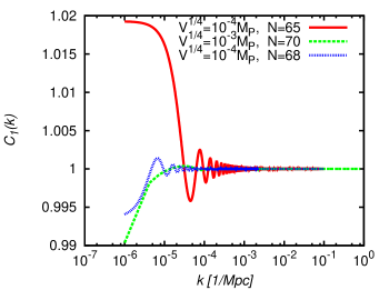
Figure 1: The function $C_{1}(k)$, corresponding to the power spectrum in the case when the collapse operator is $\hat{v}_{\textbf{k}}^{R,I}$ during inflation. We have set the value $\lambda_{\textrm{GRW}}=1.029\times 10^{-2}$ Mpc^-1 and $n_{s}=0.96$. The values of conformal time at the beginning of the inflationary regime $\tau$ corresponding to the three cases depicted (from top to bottom) are: $-\tau=7803894,115820063$ and $156745414$ Mpc. We have evaluated $C_{1}(k)$ at $\eta=\eta_{f}$, and the values of $\eta_{f}$ corresponding to the three different cases considered (from top to bottom) are: $-\eta_{f}=4.604\times 10^{-22},4.604\times 10^{-23}$ and $4.604\times 10^{-22}$ Mpc. $M_{P}$ denotes the reduced Planck mass $M_{P}\simeq 10^{18}$ GeV.

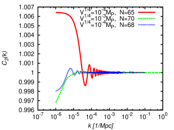
Figure 2: The function $C_{3}(k)$, corresponding to the power spectrum in the case when the collapse operator is $\hat{p}_{\textbf{k}}^{R,I}$ during inflation. We have set the value $\lambda_{\textrm{GRW}}=1.029\times 10^{-2}$ Mpc^-1 and $n_{s}=0.96$. The values of conformal time at the beginning of the inflationary regime $\tau$ corresponding to the three cases depicted (from top to bottom) are: $-\tau=7803894,115820063$ and $156745414$ Mpc. $M_{P}$ denotes the reduced Planck mass $M_{P}\simeq 10^{18}$ GeV.

Figures 1 and 2 show different plots for the functions $C_{1}(k)$ and $C_{3}(k)$, respectively. In both cases, we have considered the value of the CSL parameter as $\lambda_{\textrm{GRW}}=1.029\times 10^{-2}$ Mpc^-1, which corresponds to a value favored by experimental data Bahrami et al. (2014); Vinante et al. (2015); Toros and Bassi (2016a); Toros and Bassi (2016b). The various plots in each figure correspond to different values of the characteristic energy of inflation $V^{1/4}$, and the total $e$-foldings $N$ that inflation is assumed to last, which also set the values of $\tau$ and $\eta_{f}$. The values of $k$ considered correspond to these of observational interest, i.e. we consider $k$ in the range from $10^{-6}$ to $10^{-1}$ Mpc^-1.

As we can observe, the functions $C_{1}(k)$ and $C_{3}(k)$ exhibit an oscillatory behavior around the unit. For increasing values of $k$, the oscillations decrease in amplitude. However, we note that even for decreasing values of $k$ the functions $C_{1}(k)$ and $C_{3}(k)$ are very close to 1. Consequently, for the chosen values of $\lambda$, $V^{1/4}$ and $N$, the functions $C_{1}(k)\simeq C_{3}(k)\simeq 1$. That means that the shape of the angular power spectrum $C_{l}$ will not be very different from the standard one, but the amplitude could vary (a complete analysis will be presented in the next section).

Additionally, the fact that $C_{1}(k)$ depends on the conformal time does not seem to affect its behavior in a significant manner. In fact, it is closely similar to the one of $C_{3}(k)$, which does not depend on the conformal time. That means that the contribution from the time dependent term (i.e. the last term in Eq. (55)), to the total value of the function $C_{1}(k)$ is negligible when $-k\eta\to 0$.

VI.2 The CSL power spectra in the QMCU

We switch now the discussion to the framework of the QMCU, i.e. cases (ii) and (iv), which correspond to selecting $\hat{v}_{\textbf{k}}^{R,I}$ or $\hat{p}_{\textbf{k}}^{R,I}$ as the collapse operator, respectively.

The scalar power spectra given in both cases, i.e. Eqs. (37) and (46), can also be written in a manner similar to the standard spectrum Eq. (49). Once again, following Refs. de Haro and Cai (2015); Elizalde et al. (2015), we choose to evaluate the spectrum at the conformal time where the pivot scale “reenters the horizon” $k_{0}=|aH|$, which happens at late times during the expansion phase of the Universe (consequently the upper limit of the integral is evaluated at $\eta\to\infty$). We approximate (for the same arguments as in the previous subsection) $\mu_{s}\simeq 3/2$ in the coefficients of the terms in expressions $F_{2}(\lambda_{k},\mu_{s})$ and $F_{4}(\lambda_{k},\mu_{s})$ (but not in the powers of $k$ as these powers are directly related to the spectral index $n_{s}$). Additionally, the parameter $\lambda_{k}$ is assumed to be $\lambda_{k}=\lambda k$ for case (ii) and $\lambda_{k}=\lambda/k$ in case (iv). Moreover, we multiply and divide by a factor of $\lambda|\tau|$ in order to properly normalize the expressions $F_{2}$ and $F_{4}$.

Henceforth, the scalar power spectrum for case (ii), Eq. (37), will be written as

$$P(k)=A_{s}\left(\frac{k}{k_{0}}\right)^{n_{s}-1}C_{2}(k)$$ (58)

where

$$A_{s}=\frac{\lambda|\tau|}{6\pi^{2}}\left(\int_{-\infty}^{\infty}\frac{d\eta}{z(\eta)^{2}}\right)^{2},\qquad n_{s}-1=12\overline{\epsilon}$$ (59)

and $C_{2}(k)\equiv F_{2}(\lambda_{k}=\lambda k,\mu_{s}\simeq 3/2)/\lambda|\tau|$; thus,

$$C_{2}(k)=\frac{1}{\lambda|\tau|}\left\{\bigg{[}1-\lambda\tau-\frac{3\lambda}{k}\sin(-k\tau)\cos(-k\tau)\bigg{]}-\frac{1}{2}\left[\frac{\lambda}{k}(-k\eta)^{n_{s}-2}+\frac{\zeta_{k}^{4-n_{s}}}{2}\cos[(4-n_{s})\theta_{k}]\right]^{-1}\right\}.$$ (60)

On the other hand, the power spectrum for case (iv), Eq. (46), will be written as

$$P(k)=A_{s}\left(\frac{k}{k_{0}}\right)^{n_{s}-1}C_{4}(k)$$ (61)

with $A_{s}$ and $n_{s}$ the same as in Eq. (59), and $C_{4}(k)\equiv F_{4}(\lambda_{k}=\lambda/k,\mu_{s}\simeq 3/2)/\lambda|\tau|$. Hence,

$$C_{4}(k) = \frac{1}{\lambda|\tau|}\bigg{\{}\bigg{[}1-\lambda\tau-\frac{5\lambda}{k}\sin(-k\tau)\cos(-k\tau)\bigg{]}$$ (62)

$$- \frac{(1+4\lambda/k)^{2}}{6(\lambda/k)(-k\eta)^{n_{s}-4}+4(\lambda/k)(-k\eta)^{n_{s}-2}+\tilde{\zeta}_{k}^{4-n_{s}}\cos[\tilde{\theta}_{k}(6-n_{s})]}\bigg{\}}.$$

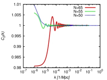
Figure 3: The function $C_{2}(k)$, corresponding to the power spectrum in the case when the collapse operator is $\hat{v}_{\textbf{k}}^{R,I}$ in the QMCU framework. We have set the value $\lambda=1.028\times 10^{-2}$ Mpc^-1 and $n_{s}=0.96$. The value of conformal time at the beginning of the quasi-matter dominated stage $\tau$ corresponding to the three cases depicted (from top to bottom) are: $-\tau=7803894,156745414$ and $115820063$ Mpc. We have evaluated $C_{2}(k)$ at $\eta=\eta_{f}$, and the values of $\eta_{f}$ corresponding to the three different cases considered (from top to bottom) are: $-\eta_{f}=5.99\times 10^{-8},1.78\times 10^{-4}$ and $1.60\times 10^{-3}$ Mpc.

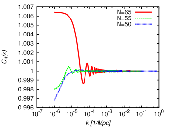
Figure 4: The function $C_{4}(k)$, corresponding to the power spectrum in the case when the collapse operator is $\hat{p}_{\textbf{k}}^{R,I}$ in the QMCU framework. We have set the value $\lambda=1.028\times 10^{-2}$ Mpc^-1 and $n_{s}=0.96$. The value of conformal time at the beginning of the quasi-matter dominated stage $\tau$ corresponding to the three cases depicted (from top to bottom) are: $-\tau=7803894,156745414$ and $115820063$ Mpc. We have evaluated $C_{4}(k)$ at $\eta=\eta_{f}$, and the values of $\eta_{f}$ corresponding to the three different cases considered (from top to bottom) are: $-\eta_{f}=5.99\times 10^{-8},1.78\times 10^{-4}$ and $1.60\times 10^{-3}$ Mpc.

As in the case of the inflationary Universe, the predicted value of the scalar spectral index $n_{s}$ is not affected by the CSL model. In fact, it has the same expression as that of the QMCU original models presented in Refs. de Haro and Cai (2015); Elizalde et al. (2015). Nevertheless, as can be seen in Eq. (59), the amplitude of the spectrum is modified by an extra factor of $\lambda|\tau|/2$ with respect to the original QMCU model, that is,

$$A_{s}=A_{s}^{\textrm{orig.}}\times\frac{\lambda|\tau|}{2}$$ (63)

In this case, $\tau$ corresponds to the beginning of the quasi-matter dominated period. Regarding the amplitude of the spectrum in the QMCU model, when the background evolution is driven by a matter dominated Universe, it can be obtained analytically working within $F(T)$ gravity or LQC. In the teleparallel $F(T)$ case, the original amplitude is

$$A_{s}^{\textrm{orig.}}=\frac{1}{3\pi^{2}}\left(\int_{-\infty}^{\infty}\frac{d\eta}{z(\eta)^{2}}\right)^{2}=\frac{\pi^{2}}{9}\frac{\rho_{c}}{\rho_{P}}$$ (64)

while in the LQC case, the original amplitude is

$$A_{s}^{\textrm{orig.}}=\frac{1}{3\pi^{2}}\left(\int_{-\infty}^{\infty}\frac{d\eta}{z(\eta)^{2}}\right)^{2}=\frac{16}{9}\frac{\rho_{c}}{\rho_{P}}\mathcal{C}^{2}$$ (65)

where $\rho_{P}$ is the Planck energy density, $\mathcal{C}\simeq 0.9159$ is Catalan’s constant and $\rho_{c}$ is called the critical density, which corresponds to the energy density at which the Universe bounces, both expressions for the amplitude can be consulted in Refs. de Haro and Cai (2015); Elizalde et al. (2015).

Thus, in order to obtain an amplitude in both cases (the teleparallel gravity case and the LQC case) that is consistent with that obtained from the CMB data (i.e. $A_{s}\simeq 10^{-9}$), and taking into account the extra factor of $\lambda|\tau|/2$ coming from the CSL model, the value of the energy density at the bouncing point must satisfy

$$\rho_{c}\simeq 10^{-9}\frac{\rho_{P}}{\lambda|\tau|}.$$ (66)

Generically $\lambda|\tau|\gg 1$; hence, the CSL model introduces an extra constriction to the QMCU, that is, $\rho_{c}\ll\rho_{P}$. In the next section we will perform a more quantitative analysis.

The functions $C_{2}(k)$ and $C_{4}(k)$ share a characteristic feature, namely they depend explicitly on $-k\eta$, which comes from a series expansion around $-k\eta\to 0$. Consequently, we choose to evaluate $\eta=\eta_{f}$ corresponding to the end of the quasi-matter domination stage or the onset of the bouncing phase. One can also define the total number of e-foldings $N\equiv\ln[a(\tau)/a(\eta_{f})]$ for the duration of the quasi-matter dominated phase; however, notice that in this case, since there is no horizon problem, there is no minimum value of $N$. Another important aspect is that if $\lambda=0$ then $C_{2}(k)=C_{4}(k)=0$. In other words, if the evolution of the state vector is completely unitary, then there are no perturbations of the spacetime at all and the state vector continues being perfectly symmetric, which is consistent with our conceptual framework.

In Figs. 3 and 4, we show different plots for the functions $C_{2}(k)$ and $C_{4}(k)$, respectively. In both cases, we have considered the value $\lambda_{\textrm{GRW}}=1.029\times 10^{-2}$ Mpc^-1. The various plots in each figure correspond to different values of $\tau$ and $\eta_{f}$. The values of $k$ considered correspond to the values of observational interest, hence, we consider $k$ in the range from $10^{-6}$ to $10^{-1}$ Mpc^-1. As we can see, the functions $C_{2}(k)$ and $C_{4}(k)$ exhibit the same oscillatory behavior around the unity as its counterparts during inflation. Also, the amplitude of each oscillation decreases for increasing values of $k$.

We end this section with a few comments regarding the dependence of the power spectrum on $\eta$ in cases (i), (ii) and (iv). In case (i), which corresponds to selecting the MS variable as the collapse operator during inflation, the term containing the $\eta$ dependence is the last one of $C_{1}(k)$ in Eq. (55). On the other hand, since the amplitude associated to the modes $\mathcal{R}_{\textbf{k}}$ is “frozen” on super-Hubble scales, the behavior of $C_{1}(k)$ will not change for super-horizon modes. As a matter of fact, the plots in Fig. 1 show that $C_{1}(k)$ is essentially a constant in the limit $-k\eta\to 0$, which means that the term containing the $\eta$ dependence is sub-dominant in such a limit. In cases (ii) and (iv), corresponding to the framework of the QMCU, the behavior of the functions $C_{2}(k)$ and $C_{4}(k)$ are very similar to that of $C_{1}(k)$ (see Figs. 3 and 4). That is, they are practically a constant in the limit $-k\eta\to 0$, which means that the terms involving $\eta$, i.e. the last terms of Eqs. (60) and (62), are sub-dominant in the super-Hubble limit. Nevertheless, since in cases (ii) and (iv) the Universe approaches a non-singular bounce, it might be the case that, when the mode “reenters the horizon” ($k\gg|aH|$) during the bouncing phase, a modification of the dynamical evolution of the functions $C_{2}(k)$ and $C_{4}(k)$ would occur. However, if the duration of the bouncing phase is short enough then one could intuitively consider that the spectrum is left unchanged (although counterexamples exist in the literature Martin and Peter (2004)). Therefore, one could perform a full analysis regarding the CSL model during the bounce within the QMCU. Nonetheless, we will take a pragmatical approach and assume that the shape of the spectrum, provided by the functions $C_{2}(k)$ and $C_{4}(k)$, survives the bouncing phase and, then, we will use the observational data to further constraint or completely discard the predicted spectra. In case that the predicted spectra are consistent with observations, one can proceed to perform the full-fledged analysis of implementing the CSL model to the QMCU during the bouncing phase and study the possible corrections that may arise from passing the perturbations through the bounce. This subject, however, will not be explored in the present paper.

In the next section, we will explore the implications of the predicted spectra using the observational data.

VII Effects on the CMB temperature spectrum and its implications on the cosmological parameters

The aim of this section is to analyze the viability of the CSL model by comparing the corresponding predictions with the ones coming from the best fit canonical model to the CMB data. In particular, we will focus on the power spectra obtained using the CSL model and its effect on the angular power spectrum.

In order to perform our analysis, we start by setting the cosmological parameters of our fiducial model, which will be used as a reference to compare with the CSL inspired spectra. The fiducial cosmology will be the best fitting flat $\Lambda$CDM model from Planck data, with the following cosmological parameters and values: baryon density in units of the critical density $\Omega_{\textrm{B}}h^{2}=0.0223$, dark matter density in units of the critical density $\Omega_{\textrm{CDM}}h^{2}=0.1188$, Hubble constant $H_{0}=67.74$ in units of km s^-1 Mpc^-1, reionization optical depth $\mathcal{T}=0.066$, the scalar spectral index $n_{s}=0.96$ and a pivot scale of $k_{0}=0.05$ Mpc^-1. These values can be found in the Table 4 presented by the latest Planck Collaboration Ade et al. (2015a).

Furthermore, we recall that the primordial power spectrum and the angular power spectrum are related by Eq. (27), i.e.

$$C_{l}=\frac{4\pi}{25}\int\frac{dk}{k}\>\Delta_{l}^{2}(k)\mathcal{P}_{s}(k).$$ (67)

Hence, we will use the CSL predicted power spectra $\mathcal{P}_{s}(k)=A_{s}(k/k_{0})^{n_{s}-1}C_{i}(k)$ with $i=1,2,3,4$, which correspond to the four different cases that we have considered so far. We will focus first on the inflationary model of the early Universe and, then, on the QMCU model. Also, note that the fiducial model corresponds to: $\mathcal{P}_{s}(k)=A_{s}(k/k_{0})^{n_{s}-1}$. The precise prediction for the angular power spectrum will be obtained by using the Boltzmann code CAMB Lewis et al. (2000), with the aforementioned cosmological parameters.

VII.1 The angular power spectrum and the CSL model during inflation

During inflation, the CSL power spectra is characterized by the functions $C_{1}(k)$ and $C_{3}(k)$, Eqs. (55) and (57), with standard spectral index $n_{s}-1=-4\epsilon+2\delta$ and amplitude

$$A_{s}=\left(\frac{V\lambda|\tau|}{12\pi^{2}M_{P}^{4}\epsilon}\right)\bigg{|}_{k_{0}=aH}$$ (68)

The output of the CAMB code, that is, the temperature autocorrelation power spectrum of the fiducial model and the one provided by the CSL model during inflation are indistinguishable; thus, we have decided not to show the plots. Instead, we present the the relative difference, which we define as

$$S(l)\equiv\frac{|C_{l}^{\textrm{CSL}}-C_{l}^{\textrm{fiducial}}|}{C_{l}^{\textrm{fiducial}}}$$ (69)

Figure 5 shows the relative difference between both predictions. On the left, we have chosen $\hat{v}_{\textbf{k}}^{R,I}$ as the collapse operator while on the right we have chosen $\hat{p}_{\textbf{k}}^{R,I}$. In both cases, we have set an energy scale of $10^{-5}M_{P}$ for the energy at which inflation ends, and a total amount of inflation corresponding to 65 $e$-foldings.

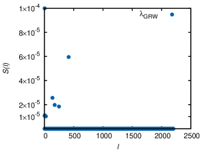
Figure 5: The relative difference $S(l)$ [defined in Eq. (69)] between the angular power spectrum predicted using the fiducial model and the one provided by the CSL model during inflation. Left: $\hat{v}_{\textbf{k}}^{R,I}$ as the collapse operator. Right: $\hat{p}_{\textbf{k}}^{R,I}$ as the collapse operator. For the CSL model, we have chosen the value of $\lambda_{\textrm{GRW}}=1.029\times 10^{-2}$ Mpc^-1. Also, we have assumed that inflation ends at an energy scale of $10^{-5}M_{P}$ and a total amount of inflation corresponding to $N=65$, i.e. $\tau=7.8\times 10^{7}$ Mpc and $\eta_{f}=4.6\times 10^{-21}$ Mpc. Other values of $\lambda$ were plotted (not shown) achieving an excellent fit, but they are observationally ruled out by their $\epsilon$ and $r$ values predicted. See Table 1 and text for details.

We observe that the relative difference between the fiducial spectrum and the one predicted using the CSL model with, for instance $\lambda_{\textrm{GRW}}$, is practically null (the highest difference is around $0.01\%$). This statement applies to both elections of the collapse operator and for other $\lambda$ values listed in Table 1 (not shown in the figure).

We have also checked that the essentially null relative difference between the fiducial model and the CSL model during inflation is also present in the $E$ polarization autocorrelation power spectrum $C_{l}^{\textrm{EE}}$ and the temperature polarization cross correlation power spectrum $C_{l}^{\textrm{TE}}$.

On the other hand, the amplitude of the power spectrum $A_{s}$ consistent with the CMB data is $A_{s}\simeq 10^{-9}$ Ade et al. (2015a). Henceforth, the amplitude obtained using the CSL model, as shown in Eq. (68), must satisfy

$$10^{-9}\simeq\left(\frac{V\lambda|\tau|}{12\pi^{2}M_{P}^{4}\epsilon}\right)\bigg{|}_{k_{0}=aH}$$ (70)

Clearly, different values of $\lambda$ will have an effect on the amplitude of the spectrum.

Assuming that the pivot scale $k_{0}$ crosses the Hubble radius at an energy scale of $V_{0}^{1/4}=10^{-4}M_{P}$ (i.e. one order of magnitude less than the presumed energy at which inflation ends), an estimate for $\epsilon$ can be calculated. Therefore, the above equation leads to

$$\epsilon\simeq\frac{\lambda|\tau|10^{-7}}{12\pi^{2}}.$$ (71)

Table 1 shows the different values of $\epsilon$ obtained by considering several $\lambda$ values. Also, in the same table, we provide an estimate for the tensor-to-scalar ratio $r$ (recall that the CSL model predicts the same relation as standard inflation, i.e $r=16\epsilon$). From Table 1, it can be seen that only the value corresponding to $\lambda_{\textrm{GRW}}$ is consistent with both, the observed shape and amplitude of the spectrum. In particular, assuming a characteristic energy scale of inflation of $10^{-4}M_{P}\simeq 10^{14}$ GeV, a total amount of inflation corresponding to $N=65$, and the value of $\lambda_{\textrm{GRW}}$, we obtain an angular spectrum with a shape and an amplitude that is indistinguishable from the fiducial model, which we know is consistent with the observational data. The amplitude of the spectrum for this particular set of values leads to an estimate for the slow roll parameter and the tensor-to-scalar ratio of $\epsilon\simeq 10^{-4}$ and $r\simeq 10^{-2}$, respectively. Those values of $\epsilon$ and $r$ are consistent with the ones presented by the latest results of the Planck Collaboration Ade et al. (2015b).

Table 1: Estimation of $\epsilon$ from Eq. (71). We have used $|\tau|=7.8\times 10^{7}$ Mpc, which corresponds to $V^{1/4}=10^{14}$ GeV and $N=65$, and the four values of $\lambda$ shown below. Also, we have estimated the tensor-to-scalar ratio using $r=16\epsilon$. Note that only the $\lambda_{\textrm{GRW}}$ case is compatible with the latest observations from Planck Collaboration Ade et al. (2015a).

$\lambda$ type	$\lambda$ [s-1]	$\lambda$ [Mpc-1]	$\epsilon$	$r$
$\lambda_{\textrm{GRW}}$	$10^{-16}$	$1.029\times 10^{-2}$	$6.77\times 10^{-4}$	0.01
$\lambda_{1}$	$10^{-12}$	102.9	6.77 (not compatible)	108 (not compatible)
$\lambda_{2}$	$10^{-10}$	10293	678 (not compatible)	10848 (not compatible)
$\lambda_{\textrm{Adler}}$	$10^{-8}$	1029378	67793 (not compatible)	1084688 (not compatible)

It is also instructive to mention that, if future observations confirm the results of the BICEP2 Collaboration Ade et al. (2014), i.e. $r\simeq 0.2$, then the value of $\lambda_{\textrm{GRW}}$ would not be compatible with the values of $V$ and $N$ used in Table 1. In fact, the $\lambda$ value that might be compatible would be one such that $\lambda\ll\lambda_{\textrm{GRW}}$. That would open a new range of parameter space to explore in addition to considering other experimental setups different from cosmological ones Toros and Bassi (2016a); Toros and Bassi (2016b).

VII.2 The angular power spectrum and the CSL model during the quasi-matter contracting phase

In the QMCU framework, the power spectra are characterized by the functions $C_{2}(k)$ and $C_{4}(k)$, i.e. Eqs. (60) and (62), respectively. The predicted scalar spectral index is $n_{s}-1=12\overline{\epsilon}$, and the amplitude is given by

$$A_{s}\simeq\frac{\rho_{c}}{\rho_{P}}\frac{\lambda|\tau|}{2}.$$ (72)

Notice we have approximated the integral that appears in the amplitude, corresponding to Eq. (59), by $\rho_{c}/\rho_{P}$ [see Eqs. (64) and (65)].

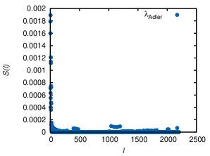
Figure 6: The relative difference $S(l)$ [defined in Eq. (69)] between the angular power spectrum predicted using the fiducial model and the one provided by the CSL model during the quasi-matter contracting phase. Left: $\hat{v}_{\textbf{k}}^{R,I}$ as the collapse operator. Right: $\hat{p}_{\textbf{k}}^{R,I}$ as the collapse operator. For the CSL model, we have chosen, as an illustrative example, the value of $\lambda_{\textrm{Adler}}=1029378$ Mpc^-1. Also, we have assumed that the quasi-matter contracting phase begins at conformal time $|\tau|=1.15\times 10^{8}$ Mpc and lasts a total amount of $N=50$ $e$-foldings, with $-\eta_{f}=1.6\times 10^{-3}$ Mpc. Other values of $\lambda$ listed in Table 2 also achieve an excellent fit (not shown), but the analysis done in this work does not allow prefer one value over another.

The output of the CAMB code, that is, the temperature autocorrelation power spectrum of the fiducial model and the one provided by the CSL model during the QMCU are also indistinguishable. Thus, we present again the relative difference defined in Eq. (69) where now $C_{l}^{\textrm{CSL}}$ corresponds to the angular power spectrum during the QMCU.

Figure 6 shows the relative difference between both predictions. On the left, we have chosen $\hat{v}_{\textbf{k}}^{R,I}$ as the collapse operator while on the right we have chosen $\hat{p}_{\textbf{k}}^{R,I}$. In both cases, we have assumed a total duration of $50$ $e$-foldings for the quasi-matter contracting phase and a conformal time $|\tau|\simeq 10^{8}$ Mpc corresponding to the beginning of the contracting stage. We show only the plot of $S(l)$ corresponding to the value of $\lambda_{\textrm{Adler}}$ merely as an illustrative example; the plots for the values corresponding to $\lambda_{1}$, $\lambda_{2}$, $\lambda_{\textrm{GRW}}$ follow the exactly same behavior as the one shown in Fig. 6.

We found no difference between the fiducial spectrum and the one provided by the CSL model for the four values of $\lambda$ listed in Table 2; the highest relative difference is around $0.1\%$. This statement applies to both elections of the collapse operator. Finally, we have also checked that the essentially null relative difference between the fiducial model and the CSL model during the QMCU is also present in the $E$ polarization autocorrelation power spectrum $C_{l}^{\textrm{EE}}$ and the temperature polarization cross correlation power spectrum $C_{l}^{\textrm{TE}}$.

On the other hand, the amplitude of the power spectrum $A_{s}$ consistent with the CMB data is $A_{s}\simeq 10^{-9}$ Ade et al. (2015a). Therefore, the ratio $\rho_{c}/\rho_{P}$, obtained using the CSL model, as shown in Eq. (72), must satisfy

$$\frac{\rho_{c}}{\rho_{P}}\simeq\kappa_{1}\qquad\textrm{where}\qquad\kappa_{1}\equiv\frac{2}{\lambda|\tau|}\times 10^{-9}.$$ (73)

Consequently, an estimate for the energy scale of the critical energy $E_{c}$ is

$$E_{c}\simeq 10^{\kappa_{2}}M_{P}\qquad\textrm{where}\qquad\kappa_{2}\equiv\frac{1}{4}\log\kappa_{1}.$$ (74)

In Table 2, we show the different values of $\kappa_{1}$ and $\kappa_{2}$ by using the chosen $\lambda$ values, with $|\tau|=1.15\times 10^{8}$ Mpc. We infer that the four values of $\lambda$ considered are consistent with a critical energy scale in the range $(10^{-3}M_{P},10^{-6}M_{P})$.

Table 2: Estimation of $\kappa_{1}$ and $\kappa_{2}$ defined in Eqs. (73) and (74) respectively. We have used $|\tau|\simeq 10^{8}$ Mpc and the four values of $\lambda$ shown below. Also we have estimated the quantities $\lambda|\tau|$.

$\lambda$ type	$\lambda$ [s-1]	$\lambda$ [Mpc-1]	$\lambda|\tau|$	$\kappa_{1}$	$\kappa_{2}$
$\lambda_{\textrm{GRW}}$	$10^{-16}$	$1.029\times 10^{-2}$	$1.029\times 10^{6}$	$10^{-15}$	-3.75
$\lambda_{1}$	$10^{-12}$	102.9	$1.029\times 10^{10}$	$10^{-19}$	-4.75
$\lambda_{2}$	$10^{-10}$	10293	$1.029\times 10^{12}$	$10^{-21}$	-5.25
$\lambda_{\textrm{Adler}}$	$10^{-8}$	1029378	$1.029\times 10^{14}$	$10^{-23}$	-5.75

It is worthwhile to mention that, in the QMCU, the spectral index $n_{s}$ and the tensor-to-scalar ratio $r$ are not related each other as in the standard inflationary paradigm [see Eqs. (43) and (59)]. However, the spectral index, along with the running of the spectral index $\alpha_{s}\equiv dn_{s}/d\ln k$, are the two main parameters of the QMCU model used to compare with the observational data Elizalde et al. (2015); de Haro and Cai (2015); de Haro and Amorós (2015). The CSL model applied to the QMCU does not affect those parameters. The only observable affected by the CSL model is the amplitude of the spectrum (which is not related to the parameter $r$ as in the standard spectrum). Consequently, in order to put an upper bound to the energy scale at which the bouncing phase begins, and which would be equivalent to set a constraint on the parameter $\lambda$, one should consider a specific theoretical model of the QMCU (i.e. to choose a specific dynamics and a potential of the field $\varphi$). Therefore, in the QMCU, and with the same degree of accuracy of past works dealing with the same model, all of the four values of the CSL parameter $\lambda$ considered here yield consistent predictions with observational data; specifically, the predictions regarding the shape of the spectrum, the scalar spectral index and the running of the spectral index.

On the other hand, note that the information that could discriminate among different values of $\lambda$ is codified in the amplitude of the spectrum. The predicted amplitude of the spectrum depends on the critical energy density $\rho_{c}$ (the value of the energy density at the bouncing time), which is model dependent.

VIII Conclusions

The CSL model is a physical mechanism that attempts to provide a solution to the measurement problem of Quantum Mechanics by modifying the Schrödinger equation. The CSL model can be referred as an objective reduction mechanism or “effective collapse” of the wave function, and one of the main elements of this model is the collapse operator, i.e. the operator whose eigenstates correspond to the evolved states by the collapse mechanism. Also, in principle, it is possible to apply such a mechanism to any physical system.

In this work, we have applied the CSL model to the early Universe by considering two cosmological models: the matter bounce scenario (MBS) and standard slow roll inflation. Additionally, we have considered two different collapse schemes, one in which the field variable (given in terms of the Mukhanov-Sasaki variable) serves as the collapse operator, and other scheme where the collapse operator is the conjugated momentum.

In all cases, we have found a prediction for the primordial power spectrum, which is a function of the standard parameters of each cosmological model, and also of the CSL parameter $\lambda$. Although the exact expressions for the primordial power spectra are different in each case, there are features that are essentially the same as its standard–non-collapse–counterparts. Specifically, the predictions for the scalar spectral index and the tensor-to-scalar ratio are exactly the same as the ones given in the MBS and slow roll inflation without collapse. On the other hand, in each case, the shape of the spectrum is modified by a function of the wave number $k$, associated to the modes of the field, and by the inclusion of the $\lambda$ parameter. However, for a suitable choice of values corresponding to the parameters of the cosmological models, there is no significant change in the prediction for the CMB angular power spectrum (i.e. the $C_{l}$’s) that can be distinguished from the canonical flat $\Lambda$CDM model.

Meanwhile, the prediction for the amplitude of the spectrum is modified directly by the parameter $\lambda$. We have empirically explored the range of values of $\lambda$, from the originally value suggested by Ghirardi-Rimini-Weber (GRW) $\lambda_{\textrm{GRW}}\simeq 10^{-16}$ s^-1 Ghirardi et al. (1986), to the one given by Adler $\lambda_{\textrm{Adler}}\simeq 10^{-8}$ s^-1 Adler (2007). In the case of slow roll inflation, we have found that for a characteristic energy scale of $10^{14}$ GeV and a total amount of inflation of 65 $e$-folds, only the value suggested by GRW is compatible with the observational bound of the amplitude; other values of $\lambda$ greater than $\lambda_{\textrm{GRW}}$, e.g. $\lambda_{\textrm{Adler}}$, cannot be made compatible with the observed amplitude (because that would require values for the slow roll parameter such that $\epsilon>1$). In the MBS case, we have found that the modification in the predicted amplitude of the spectrum, given by the $\lambda$ parameter, causes that the critical energy density $\rho_{c}$, i.e. the energy density at which the bouncing phase begins, to be several orders of magnitude less than the Planck energy density $\rho_{P}$. The precise number of orders of magnitude varies according to the value of $\lambda$. For instance, by assuming $\lambda_{\textrm{GRW}}$ and a total amount of $\sim 50$ $e$-folds for the matter dominated contracting phase, we have $\rho_{c}\simeq 10^{-15}\rho_{P}$. The latter relation is obtained by requiring the compatibility between the predicted amplitude of the scalar power spectrum and the one from the Planck CMB data $A_{s}\sim 10^{-9}$.

In conclusion, it was possible to incorporate the CSL model into the cosmological context again, in particular when dealing with the quantum-to-classical transition of the primordial inhomogeneities. Moreover, it is remarkable that our implementation of the CSL model yields predictions that are also in agreement with experiments in the regimes so far investigated empirically. Those experiments involve values of the CSL parameter $\lambda$ that have been tested in laboratory settings, quite disengaged from the cosmological framework. We acknowledge that at this stage, the application of CSL model to the early Universe, as done in this manuscript, can be seen as an ad hoc employment. However, the fact that the predictions can be empirically tested make us hopeful that future studies will overcome the perceived shortcomings.

Appendix A Calculations of Section V

In this Appendix, we provide a sketch of the computational steps that led to the results presented in Sect. V. In the first half of this Appendix, we will focus on cases (i) and (iii), which correspond to selecting the MS variable as the collapse operator during inflation and the QMCU, respectively. The second half will contain the details according to cases (ii) and (iv), corresponding to selecting $\hat{p}_{\textbf{k}}^{R,I}$ as the collapse operator during inflation and the QMCU, respectively.

A.1 The field $\hat{v}_{\textbf{k}}$ as the collapse operator

We will proceed the calculation of the scalar power spectrum by dealing simultaneously with the inflationary and the QMCU frameworks; and finally, we will argue that the computation is similar for the tensor power spectrum.

In order to obtain the scalar power spectrum, we will use Eq. (33). Let us focus first on the second term on the right hand side in that equation, which can be obtained by using the CSL evolution equation (31). Recall that, since in this case $\hat{\varTheta}_{\textbf{k}}=\hat{v}_{\textbf{k}}$, it will be convenient to work with the wave function in the field representation Eq. (13). The CSL evolution equation leads to the following equation of motion:

$$A_{k}^{\prime}=\frac{ik^{2}}{2}+\lambda_{k}-\frac{2\beta}{\eta}A_{k}-2iA_{k}^{2}.$$ (75)

The previous equation is solved by performing the change of variable $A_{k}(\eta)\equiv f_{k}^{\prime}(\eta)/[2if_{k}(\eta)]$, resulting in a Bessel differential equation for $f_{k}(\eta)$. After solving such an equation, and returning to the original variable $A_{k}$, we obtain

$$A_{k}(\eta)=\frac{q}{2i}\left[\frac{-J_{m-1}(-q\eta)-e^{-i\pi m}J_{1-m}(-q\eta)}{J_{m}(-q\eta)-e^{-i\pi m}J_{-m}(-q\eta)}\right],$$ (76)

being $q^{2}\equiv k^{2}(1-2i\lambda_{k}/k^{2})$, and where the initial condition for the Bunch-Davies vacuum $A_{k}(\tau)=k/2$ was used (we remind the reader that $\tau$ corresponds to the conformal time at the beginning of the contraction phase or the exponential expansion). The function $J_{m}$ is a Bessel function of the first kind of order $m\equiv 1/2-\beta$ [recall that $\beta$ is defined in Eq. (10)].

We now expand $A_{k}(\eta)$ in the limit where the proper wavelength associated to the modes becomes larger than the Hubble radius $H^{-1}$, that is, in the limit $-q\eta\to 0$ (provided that $\lambda_{k}\ll 1$). However, note that $\beta$ varies according whether inflation or a contracting phase is assumed. For inflation $\beta\simeq-1$ whilst for the QMCU case $\beta\simeq 2$. This implies that the dominant modes correspond to $m\simeq 3/2$ during inflation. On the contrary, in the QMCU, the dominant modes correspond to $m\simeq-3/2$. Furthermore, we are only interested in the expansion on the real part of $A_{k}(\eta)$. Therefore, for case (i) the expansion of the real part of $A_{k}(\eta)$ is

$$\text{Re}\>A_{k}(\eta)\simeq\frac{\lambda_{k}}{2k(m-1)}(-k\eta)+\zeta_{k}^{2m}\frac{\sin(\pi m+2m\theta_{k})}{\sin(\pi m)}\frac{k\pi}{2^{2m}\Gamma(m)^{2}}(-k\eta)^{2m-1},$$ (77)

and for case (ii) the corresponding expansion is

$$\text{Re}\>A_{k}(\eta)\simeq\frac{\lambda_{k}}{2k(-m-1)}(-k\eta)+\zeta_{k}^{-2m}\frac{\sin(\pi m+2m\theta_{k})}{\sin(\pi m)}\frac{k\pi}{2^{-2m}\Gamma(-m)^{2}}(-k\eta)^{-2m-1}.$$ (78)

In both cases, $\zeta_{k}$ and $\theta_{k}$ are given in Eq. (39).

Next, we focus on the first term of Eq. (33), i.e. $\overline{\langle\hat{v}_{\textbf{k}}^{2}\rangle}$. It will be useful to define the following quantities:

$$Q\equiv\overline{\langle\hat{v}_{\textbf{k}}^{2}\rangle},R\equiv\overline{\langle\hat{p}_{\textbf{k}}^{2}\rangle}\>\>\textrm{and}\>\>S\equiv\overline{\langle\hat{p}_{\textbf{k}}\hat{v}_{\textbf{k}}+\hat{v}_{\textbf{k}}\hat{p}_{\textbf{k}}\rangle}.$$ (79)

The equations of evolution for $Q,R$ and $S$ are obtained using Eq. (32), with $\hat{\varTheta}_{\textbf{k}}=\hat{v}_{\textbf{k}}$. That is,

$$Q^{\prime}=S+\frac{2\beta}{\eta}Q,\qquad R^{\prime}=-k^{2}S-\frac{2\beta}{\eta}R+\lambda_{k},\qquad S^{\prime}=2R-2k^{2}Q.$$ (80)

Therefore, we have a linear system of coupled differential equations, whose general solution is a particular solution to the system plus a solution to the homogeneous equation (with $\lambda_{k}=0$). After a long series of calculations we find:

$$Q(\eta)=(-k\eta)[C_{1}J_{n}^{2}(-k\eta)+C_{2}J_{-n}^{2}(-k\eta)+C_{3}J_{n}(-k\eta)J_{-n}(-k\eta)]+\frac{\lambda_{k}\eta}{2k^{2}},$$ (81)

with

$$n=\frac{3}{2}+\frac{2}{3}\alpha;\qquad\textrm{and}\qquad\alpha\equiv\begin{cases}3\epsilon-\frac{3}{2}\delta\>\>\textrm{if assuming the inflationary Universe }\\ -9\bar{\epsilon}\>\>\textrm{if assuming the QMCU }\\ \end{cases}$$ (82)

and the constants $C_{1},C_{2}$ and $C_{3}$ are found by imposing the initial conditions corresponding to the Bunch-Davies vacuum state: $Q(\tau)=1/(2k),R(\tau)=k/2$ and $S(\tau)=0$. Equation (81) is exact; expanding it again around $-k\eta\to 0$ yields

$$Q(\eta)\simeq\frac{\pi}{2k^{2}\sin^{2}(n\pi)}\bigg{\{}\frac{k}{2}-\frac{\lambda_{k}\tau}{2}+\frac{m\lambda_{k}}{k}\sin\Delta\cos\Delta\bigg{\}}\frac{2^{2n}}{\Gamma^{2}(1-n)}(-k\eta)^{-2n+1},$$ (83)

where

$$\Delta=-k\tau-\frac{n\pi}{2}-\frac{\pi}{4}.$$ (84)

Using the above results, we can compute the quantity $\overline{\langle\hat{v}_{\textbf{k}}\rangle^{2}}$ using Eq. (33). In case (i), we substitute Eqs. (77) and (83) into Eq. (33), obtaining

$$\overline{\langle\hat{v}_{\textbf{k}}\rangle^{2}} = Q(\eta)-\frac{1}{4\textrm{Re}A_{k}(\eta)}$$ (85)

$$\simeq \frac{\pi}{2k^{2}\sin^{2}(n\pi)}\bigg{\{}\frac{k}{2}-\frac{\lambda_{k}\tau}{2}+\frac{m\lambda_{k}}{k}\sin\Delta\cos\Delta\bigg{\}}\frac{2^{2n}}{\Gamma^{2}(1-n)}(-k\eta)^{-2n+1}$$

$$- \frac{1}{4}\left[\frac{\lambda_{k}}{2k(m-1)}(-k\eta)+\zeta_{k}^{2m}\frac{\sin(\pi m+2m\theta_{k})}{\sin(\pi m)}\frac{k\pi}{2^{2m}\Gamma(m)^{2}}(-k\eta)^{2m-1}\right]^{-1}.$$

With the expression in (85) at hand (which is valid for $\overline{\langle\hat{v}_{\textbf{k}}^{R}\rangle^{2}}$ and $\overline{\langle\hat{v}_{\textbf{k}}^{I}\rangle^{2}}$), and using Eq. (30), our predicted scalar power spectrum during inflation (at the lowest order in the slow roll parameter) is given in Eq. (35). (we have also used that during inflation $z^{2}(\eta)\simeq 2\epsilon M_{P}^{2}/(H^{2}\eta^{2})$ and $m=n=3/2+2\epsilon-\delta$).

Analogously, in case (ii), substituting Eqs. (78) and (83) into (33) yields

$$\overline{\langle\hat{v}_{\textbf{k}}\rangle^{2}} = Q(\eta)-\frac{1}{4\textrm{Re}A_{k}(\eta)}$$ (86)

$$\simeq \frac{\pi}{2k^{2}\sin^{2}(n\pi)}\bigg{\{}\frac{k}{2}-\frac{\lambda_{k}\tau}{2}+\frac{m\lambda_{k}}{k}\sin\Delta\cos\Delta\bigg{\}}\frac{2^{2n}}{\Gamma^{2}(1-n)}(-k\eta)^{-2n+1}$$

$$- \frac{1}{4}\left[\frac{\lambda_{k}}{2k(-m-1)}(-k\eta)+\zeta_{k}^{-2m}\frac{\sin(\pi m+2m\theta_{k})}{\sin(\pi m)}\frac{k\pi}{2^{-2m}\Gamma(-m)^{2}}(-k\eta)^{-2m-1}\right]^{-1}.$$

Hence, substituting the above expression in Eq. (30) yields:

$$P_{s}(k) = \frac{(-k\eta)^{-2\mu_{s}+3}}{4\pi^{2}z^{2}\eta^{2}}\bigg{\{}\frac{2^{2\mu_{s}}\pi}{\sin^{2}(\mu_{s}\pi)\Gamma^{2}(1-\mu_{s})}\bigg{[}1-\frac{\lambda_{k}\tau}{k}-\frac{3\lambda_{k}}{k^{2}}\sin(-k\tau)\cos(-k\tau)\bigg{]}$$ (87)

$$- \left[\frac{\lambda_{k}}{2(\mu_{s}-1)k^{2}}(-k\eta)^{-2\mu_{s}+2}+\frac{\zeta_{k}^{2\mu_{s}}\pi\sin(\pi\mu_{s}+2\mu_{s}\theta_{k})}{\sin(\pi\mu_{s})2^{2\mu_{s}}\Gamma^{2}(\mu_{s})}\right]^{-1}\bigg{\}},\qquad\mu_{s}\equiv\frac{3}{2}-6\bar{\epsilon}$$

where we have used $m=-n=3/2-6\bar{\epsilon}$. As argued in Refs. Elizalde et al. (2015); de Haro and Cai (2015), during the quasi-matter contracting phase $z\simeq\eta^{2}/(3\sqrt{3})$ and $|aH|=-2/\eta$, which implies that Eq. (87) can be written as in the final form of the power spectrum presented in Eq. (37)

Let us focus now on the tensor modes. The action for the tensor perturbations is obtained from the Einstein-Hilbert action by expanding the tensor perturbations $h_{ij}(\textbf{x},\eta)$ up to second-order Mukhanov et al. (1992). The resulting action for the tensor field $h_{ij}(\textbf{x},\eta)$ can be expressed in terms of its Fourier modes $h_{ij}(\textbf{k},\eta)=h_{\textbf{k}}(\eta)e_{ij}(\textbf{k})$, with $e_{ij}(\textbf{k})$ representing a time-independent polarization tensor. Performing the change of variable

$$h_{\textbf{k}}(\eta)\equiv\frac{2}{M_{P}(e^{i}_{\,j}e^{j}_{\,i})^{1/2}}\frac{v_{\textbf{k}}(\eta)}{a(\eta)},$$ (88)

the action can be written as $\delta^{(2)}S_{h}=\frac{1}{2}\int d\eta\>d^{3}\textbf{k}\>\mathcal{L}_{h}$, where

$$\mathcal{L}_{h}=v_{\textbf{k}}^{\prime}v_{\textbf{k}}^{\star^{\prime}}-k^{2}v_{\textbf{k}}v_{\textbf{k}}^{\star}-\frac{a^{\prime}}{a}\left(v_{\textbf{k}}v_{\textbf{k}}^{\star^{\prime}}+v_{\textbf{k}}^{\prime}v_{\textbf{k}}^{\star}\right)+\left(\frac{a^{\prime}}{a}\right)^{2}v_{\textbf{k}}v_{\textbf{k}}^{\star}.$$ (89)

The Lagrangian in Eq. (9), and the one in Eq. (89), share the same structure. In particular, if one replaces $z^{\prime}/z\to a^{\prime}/a$ in Eq. (9), one obtains Eq. (89). Thus, the preceding calculations can be directly employed to obtain the tensor power spectrum by replacing $z^{\prime}/z\to a^{\prime}/a$ in the whole procedure. The explicit form of this last quantity is

$$\frac{a^{\prime}(\eta)}{a(\eta)}=\frac{\tilde{\beta}}{\eta};\qquad\textrm{where}\qquad\tilde{\beta}\equiv\begin{cases}-(1+\epsilon)\>\>\textrm{if assuming the inflationary Universe }\\ 2(1-3\overline{\epsilon})\>\>\textrm{if assuming the QMCU }.\\ \end{cases}$$ (90)

Consequently, the replacement $\beta\to\tilde{\beta}$, in the equations of the present subsection, allows us to obtain the tensor power spectra shown in Eqs. (40) and (42).

A.2 The momentum $\hat{p}_{\textbf{k}}$ as the collapse operator

In the rest of this Appendix, we will present the mathematical details for obtaining the scalar and tensor power spectra, using the CSL model, when the collapse operator is $\hat{p}_{\textbf{k}}$. As in the previous subsection, we will use the framework provided by the inflationary Universe and the QMCU simultaneously. This will complete the computation of the power spectra for the last two cases mentioned at the beginning of Sect. V, i.e. cases (iii) and (iv).

Since in this subsection we are considering that the collapse operator is the momentum operator, $\hat{\varTheta}_{\textbf{k}}=\hat{p}_{\textbf{k}}^{R,I}$, it is convenient to work with the wave function in the momentum representation, Eq. (14). Moreover, as argued at the beginning of this section, in that representation, the quantities of interest, namely $\overline{\langle\hat{v}_{\textbf{k}}^{R}\rangle^{2}}$ and $\overline{\langle\hat{v}_{\textbf{k}}^{I}\rangle^{2}}$, can be calculated using Eq. (34). Furthermore, in spite of the collapse operator being the momentum operator, the calculations of the previous subsection serve as a blueprint for the computations in this subsection. Once again, we will proceed by omitting the indexes $R$,$I$.

Let us focus first on the second term of the right hand side of Eq. (34), i.e. $|\tilde{A}_{k}(\eta)|^{2}/\textrm{Re}[\tilde{A}_{k}(\eta)]$. The motion equation for $\tilde{A}_{k}(\eta)$ is obtained from the CSL Eq. (31), which leads to

$$\tilde{A}_{k}^{\prime}(\eta)=\frac{i}{2}+\lambda_{k}+\frac{2\beta}{\eta}\tilde{A}_{k}-2ik^{2}\tilde{A}_{k}(\eta)^{2}.$$ (91)

Performing the change of variable $\tilde{A}_{k}\equiv g_{k}^{\prime}(\eta)/[2ik^{2}g_{k}(\eta)]$ in the last equation, results in a Bessel differential equation for $g_{k}(\eta)$. Now, using such a solution and returning to the original variable, we have

$$\tilde{A}_{k}(\eta)=\frac{q}{2ik^{2}}\left[\frac{J_{m+1}(-q\eta)+e^{-im\pi}J_{-m-1}(-q\eta)}{J_{m}(-q\eta)-e^{-im\pi}J_{-m}(-q\eta)}\right],\qquad\qquad m\equiv-\frac{1}{2}-\beta,$$ (92)

where $q^{2}\equiv k^{2}(1-2i\lambda_{k})$. Also, we have used the initial condition provided by the Bunch-Davies vacuum, which is $\tilde{A}_{k}(\tau)=1/2k$ with $\tau\to-\infty$. Do not confuse the $m$ of Eq. (92) with the one of the previous subsection.

The next step is to perform the expansion for $-q\eta\to 0$. Note that if we consider the inflationary Universe, then $\beta\simeq-1$, which means that $m\simeq 1/2$. On the other hand, for the QMCU case $\beta\simeq 2$, which implies that $m\simeq-5/2$ [note that $\beta$ is defined in Eq. (10)].

In other words, for case (iii), we have the following expansion

$$\frac{|\tilde{A}_{k}(\eta)|^{2}}{\text{Re}[A_{k}(\eta)]}\simeq\frac{\sin(\pi m)\Gamma^{2}(m+1)2^{2m}\tilde{\zeta}_{k}^{-2m}(-k\eta)^{-2m-1}}{k\sin(2m\tilde{\theta}_{k}+\pi m)\pi}.$$ (93)

And in case (iv), the corresponding expansion results,

$$\frac{|\tilde{A}_{k}(\eta)|^{2}}{\text{Re}[A_{k}(\eta)]}\simeq\frac{c_{1}\tilde{\zeta}_{k}^{2}}{2k}\left[\frac{1+c_{2}2\tilde{\zeta}_{k}^{2}\cos(2\tilde{\theta}_{k})(-k\eta)^{2}+c_{2}2\tilde{\zeta}_{k}^{2}\cos[2(m+1)\tilde{\theta}_{k}+\pi m](-k\eta)^{-2m-2}}{\sin(2\tilde{\theta}_{k})(-k\eta)^{2m+2}+c_{2}\tilde{\zeta}_{k}^{2}\sin(4\tilde{\theta}_{k})(-k\eta)^{2m+4}-c_{3}\tilde{\zeta}_{k}^{-2m-2}\sin[2m\tilde{\theta}_{k}+\pi m]}\right](-k\eta)^{2m+3}$$ (94)

where

$$c_{1}\equiv\frac{1}{2(m+1)},\qquad\qquad c_{2}\equiv\frac{1}{2^{2}(m+1)(m+2)},\qquad\qquad c_{3}\equiv\frac{2^{2m+2}\Gamma(m+2)}{\Gamma(-m)}.$$ (95)

In both cases, the definitions of the quantities $\tilde{\zeta_{k}}$ and $\tilde{\theta}_{k}$ are given in Eq. (48).

Now, we have to obtain the first term of the right hand side of Eq. (34), that is, $\overline{\langle\hat{v}_{\textbf{k}}^{2}\rangle}$. We will employ the same procedure as in the previous subsection. We use the previous definitions for the quantities $Q(\eta)$,$R(\eta)$ and $S(\eta)$ Eq. (79) and Eq. (32) but taking into account that $\varTheta_{\textbf{k}}^{R,I}=\hat{p}_{\textbf{k}}^{R,I}$. Thus, the evolution equations are:

$$Q^{\prime}=S+\frac{2\beta}{\eta}Q+\lambda_{k},\enskip R^{\prime}=-k^{2}S-\frac{2\beta}{\eta}R,\enskip S^{\prime}=2R-2k^{2}Q.$$ (96)

Those equations are solved using the initial conditions provided by $Q(\tau)=1/(2k)$, $R(\tau)=k/2$ and $S(\tau)=0$.

We are mainly interested in the solution for $Q(\eta)\equiv\overline{\langle\hat{v}_{\textbf{k}}^{2}\rangle}$ [which is the first term on the right hand side of Eq. (34)]. Then, performing the series expansion to the lowest order around $-k\eta\to 0$ yields

$$Q(\eta)\simeq\frac{\pi}{2k^{2}\sin^{2}(n\pi)}\bigg{\{}\frac{k}{2}-\frac{k^{2}\lambda_{k}\tau}{2}+{mk\lambda_{k}}\sin\Delta\cos\Delta\bigg{\}}\frac{2^{2n}}{\Gamma^{2}(1-n)}(-k\eta)^{-2n+1}$$ (97)

where $\Delta=-k\tau-\frac{n\pi}{2}-\frac{\pi}{4}$ and $n$ is exactly the same as the one defined in Eq. (82).

We are now in position to compute the scalar power spectrum. For case (iii), substituting Eqs. (93) and (97) into Eq. (34) yields

$$\overline{\langle\hat{v}_{\textbf{k}}\rangle^{2}} = Q(\eta)-\frac{|A_{k}(\eta)|^{2}}{\textrm{Re}A_{k}(\eta)}$$ (98)

$$\simeq \frac{\pi}{2k^{2}\sin^{2}(n\pi)}\bigg{\{}\frac{k}{2}-\frac{k^{2}\lambda_{k}\tau}{2}+{mk\lambda_{k}}\sin\Delta\cos\Delta\bigg{\}}\frac{2^{2n}}{\Gamma^{2}(1-n)}(-k\eta)^{-2n+1}$$

$$- \frac{\sin(\pi m)\Gamma^{2}(m+1)2^{2m}\zeta_{k}^{-2m}(-k\eta)^{-2m-1}}{k\sin(2m\theta_{k}+\pi m)\pi}.$$

In addition, by noting that $m=1/2+2\epsilon-\delta$ and $n=3/2+2\epsilon-\delta$, we substitute Eq. (98) in Eq. (30), which results in the final expression for the power spectrum shown in Eq. (44).

For case (iv), we substitute Eq. (94) and Eq. (97) into Eq. (34) which results in

$$\overline{\langle\hat{v}_{\textbf{k}}\rangle^{2}} = Q(\eta)-\frac{|A_{k}(\eta)|^{2}}{\textrm{Re}A_{k}(\eta)}$$ (99)

$$\simeq \frac{\pi}{2k^{2}\sin^{2}(n\pi)}\bigg{\{}\frac{k}{2}-\frac{k^{2}\lambda_{k}\tau}{2}+{mk\lambda_{k}}\sin\Delta\cos\Delta\bigg{\}}\frac{2^{2n}}{\Gamma^{2}(1-n)}(-k\eta)^{-2n+1}$$

$$- \frac{c_{1}\zeta_{k}^{2}}{2k}\left[\frac{1+c_{2}2\zeta_{k}^{2}\cos(2\theta_{k})(-k\eta)^{2}+c_{2}2\zeta_{k}^{2}\cos[2(m+1)\theta_{k}+\pi m](-k\eta)^{-2m-2}}{\sin(2\theta_{k})(-k\eta)^{2m+2}+c_{2}\zeta_{k}^{2}\sin(4\theta_{k})(-k\eta)^{2m+4}-c_{3}\zeta_{k}^{-2m-2}\sin[2m\theta_{k}+\pi m]}\right](-k\eta)^{2m+3}.$$

Since in this case $m=-5/2+6\overline{\epsilon}$ and $n=3/2-6\overline{\epsilon}$, and considering only the first dominant term in the expansion around $-k\eta\to 0$, we finally obtain the expression for the power spectrum presented in Eq. (46).

The procedure to obtain the tensor power spectra is analogous to the one outlined in the previous subsection, but clearly the difference is that $\hat{\varTheta}_{\textbf{k}}^{R,I}=\hat{p}_{\textbf{k}}^{R,I}$. In the following, we will only present the results.

For case (iii), the tensor power spectrum is given by

$$P_{t}(k)=\frac{2^{2\nu_{t}+1}H^{2}\Gamma^{2}(\nu_{t})}{M_{P}^{2}\pi^{3}}(-k\eta)^{-2\nu_{t}+1}F_{3}(\lambda_{k},\nu_{t}),\qquad\nu_{t}\equiv\frac{1}{2}+\epsilon,$$ (100)

and, consequently, the tensor-to-scalar ratio is $r=16\epsilon$, which is the same as the standard prediction of slow roll inflation.

For case (iv), the formula for the tensor power spectrum is

$$P_{t}(k)=\frac{2}{9\pi^{2}}\left(\int_{-\infty}^{\eta}\frac{d\tilde{\eta}}{z_{T}^{2}}\right)^{2}\left(\frac{k}{|aH|}\right)^{-2\mu_{t}+3}F_{4}(\lambda_{k},\mu_{t}),\qquad\mu_{t}\equiv\frac{3}{2}-6\overline{\epsilon}=\mu_{s}.$$ (101)

Therefore, the tensor-to-scalar ratio is exactly the same as the one shown in Eq. (43).

References

- Guth (1981) A. H. Guth, Phys. Rev. D23, 347 (1981).
- Starobinsky (1980) A. A. Starobinsky, Phys. Lett. B91, 99 (1980).
- Linde (1982) A. D. Linde, Phys. Lett. B108, 389 (1982).
- Albrecht and Steinhardt (1982) A. Albrecht and P. J. Steinhardt, Phys. Rev. Lett. 48, 1220 (1982).
- Ade et al. (2015a) P. A. R. Ade et al. (Planck), Planck 2015 results. XIII. Cosmological parameters (2015a), eprint 1502.01589.
- Ade et al. (2015b) P. A. R. Ade et al. (Planck), Planck 2015 results. XX. Constraints on inflation (2015b), eprint 1502.02114.
- Ade et al. (2015c) P. Ade et al. (BICEP2, Planck), Phys. Rev. Lett. 114, 101301 (2015c), eprint 1502.00612.
- Mukhanov and Chibisov (1981) V. F. Mukhanov and G. V. Chibisov, JETP Lett. 33, 532 (1981).
- Starobinsky (1983) A. A. Starobinsky, Sov.Astron.Lett. 9, 302 (1983).
- Hawking and Moss (1983) S. W. Hawking and I. G. Moss, Nucl. Phys. B224, 180 (1983).
- Bardeen et al. (1983) J. M. Bardeen, P. J. Steinhardt, and M. S. Turner, Phys. Rev. D28, 679 (1983).
- Martin and Vennin (2016) J. Martin and V. Vennin, Phys. Rev. D93, 023505 (2016), eprint 1510.04038.
- Ijjas et al. (2013) A. Ijjas, P. J. Steinhardt, and A. Loeb, Phys. Lett. B723, 261 (2013), eprint 1304.2785.
- Battefeld and Peter (2015) D. Battefeld and P. Peter, Phys. Rept. 571, 1 (2015), eprint 1406.2790.
- Vilenkin (1983) A. Vilenkin, Phys. Rev. D27, 2848 (1983).
- Martin and Brandenberger (2001) J. Martin and R. H. Brandenberger, Phys. Rev. D63, 123501 (2001), eprint hep-th/0005209.
- Ijjas et al. (2014) A. Ijjas, P. J. Steinhardt, and A. Loeb, Phys. Lett. B736, 142 (2014), eprint 1402.6980.
- Ijjas and Steinhardt (2016) A. Ijjas and P. J. Steinhardt, Class. Quant. Grav. 33, 044001 (2016), eprint 1512.09010.
- Linde (2015) A. Linde, in 100e Ecole d’Ete de Physique: Post-Planck Cosmology Les Houches, France, July 8-August 2, 2013 (2015), pp. 231–316, eprint 1402.0526.
- Guth et al. (2014) A. H. Guth, D. I. Kaiser, and Y. Nomura, Phys. Lett. B733, 112 (2014), eprint 1312.7619.
- Brandenberger (2011) R. H. Brandenberger, Int. J. Mod. Phys. Conf. Ser. 01, 67 (2011), eprint 0902.4731.
- Elizalde et al. (2015) E. Elizalde, J. Haro, and S. D. Odintsov, Phys. Rev. D91, 063522 (2015), eprint 1411.3475.
- de Haro and Cai (2015) J. de Haro and Y.-F. Cai, Gen. Rel. Grav. 47, 95 (2015), eprint 1502.03230.
- de Haro and Amorós (2015) J. de Haro and J. Amorós, J. Phys. Conf. Ser. 600, 012024 (2015), eprint 1411.7611.
- Haro (2013) J. Haro, JCAP 1311, 068 (2013), [Erratum: JCAP1405,E01(2014)], eprint 1309.0352.
- Haro and Amoros (2014) J. Haro and J. Amoros, JCAP 1412, 031 (2014), eprint 1406.0369.
- Cai (2014) Y.-F. Cai, Sci. China Phys. Mech. Astron. 57, 1414 (2014), eprint 1405.1369.
- Cai et al. (2016) Y.-F. Cai, F. Duplessis, D. A. Easson, and D.-G. Wang, Phys. Rev. D93, 043546 (2016), eprint 1512.08979.
- Kiefer and Polarski (2009) C. Kiefer and D. Polarski, Adv. Sci. Lett. 2, 164 (2009), eprint 0810.0087.
- Halliwell (1989) J. J. Halliwell, Phys. Rev. D39, 2912 (1989).
- Kiefer (2000) C. Kiefer, Nucl. Phys. Proc. Suppl. 88, 255 (2000), eprint astro-ph/0006252.
- Polarski and Starobinsky (1996) D. Polarski and A. A. Starobinsky, Class. Quant. Grav. 13, 377 (1996), eprint gr-qc/9504030.
- Grishchuk and Sidorov (1990) L. P. Grishchuk and Yu. V. Sidorov, Phys. Rev. D42, 3413 (1990).
- Sudarsky (2011) D. Sudarsky, International Journal of Modern Physics D 20, 509 (2011), eprint 0906.0315.
- Landau et al. (2013) S. J. Landau, G. León, and D. Sudarsky, Phys. Rev. D 88, 023526 (2013), eprint 1107.3054.
- Mukhanov (2005) V. Mukhanov, Physical Foundations of Cosmology (New York: Cambridge University Press, 2005).
- Weinberg (2008) S. Weinberg, Cosmology (New York: Oxford University Press, 2008).
- Pinto-Neto et al. (2012) N. Pinto-Neto, G. Santos, and W. Struyve, Phys. Rev. D85, 083506 (2012), eprint 1110.1339.
- Valentini (2010) A. Valentini, Phys. Rev. D82, 063513 (2010), eprint 0805.0163.
- Goldstein et al. (2015) S. Goldstein, W. Struyve, and R. Tumulka, The Bohmian Approach to the Problems of Cosmological Quantum Fluctuations (2015), eprint 1508.01017.
- Ghirardi et al. (1986) G. Ghirardi, A. Rimini, and T. Weber, Phys.Rev. D34, 470 (1986).
- Pearle (1989) P. M. Pearle, Phys.Rev. A39, 2277 (1989).
- Bassi and Ghirardi (2003) A. Bassi and G. C. Ghirardi, Phys.Rept. 379, 257 (2003), eprint quant-ph/0302164.
- Bassi et al. (2013) A. Bassi, K. Lochan, S. Satin, T. P. Singh, and H. Ulbricht, Rev. Mod. Phys. 85, 471 (2013), eprint 1204.4325.
- Bassi et al. (2012) A. Bassi, K. Lochan, S. Satin, T. P. Singh, and H. Ulbricht, Stochastic Methods and Dynamical Wave-function Collapse (2012), eprint 1212.5535.
- Martin et al. (2012) J. Martin, V. Vennin, and P. Peter, Phys.Rev. D 86, 103524 (2012), eprint 1207.2086.
- Cañate et al. (2013) P. Cañate, P. Pearle, and D. Sudarsky, Phys.Rev. D 87, 104024 (2013), eprint 1211.3463.
- Das et al. (2013) S. Das, K. Lochan, S. Sahu, and T. P. Singh, Phys. Rev. D88, 085020 (2013), [Erratum: Phys. Rev.D89,no.10,109902(2014)], eprint 1304.5094.
- Das et al. (2014) S. Das, S. Sahu, S. Banerjee, and T. P. Singh, Phys. Rev. D90, 043503 (2014), eprint 1404.5740.
- León and Bengochea (2016) G. León and G. R. Bengochea, Eur. Phys. J. C76, 29 (2016), eprint 1502.04907.
- Alexander et al. (2016) S. Alexander, D. Jyoti, and J. Magueijo (2016), eprint 1602.01216.
- Perez et al. (2006) A. Perez, H. Sahlmann, and D. Sudarsky, Class. Quant. Grav. 23, 2317 (2006), eprint gr-qc/0508100.
- Diez-Tejedor et al. (2012) A. Diez-Tejedor, G. Leon, and D. Sudarsky, Gen.Rel.Grav. 44, 2965 (2012), eprint 1106.1176.
- Kodama and Sasaki (1984) H. Kodama and M. Sasaki, Progress of Theoretical Physics Supplement 78, 1 (1984).
- Toros and Bassi (2016a) M. Toros and A. Bassi, Bounds on Collapse Models from Matter-Wave Interferometry (2016a), eprint 1601.03672.
- Toros and Bassi (2016b) M. Toros and A. Bassi, Bounds on Collapse Models from Matter-Wave Interferometry: Calculational details (2016b), eprint 1601.02931.
- Ghirardi et al. (1990) G. C. Ghirardi, P. M. Pearle, and A. Rimini, Phys. Rev. A42, 78 (1990).
- Adler (2007) S. L. Adler, J. Phys. A40, 2935 (2007), [Erratum: J. Phys.A40,13501(2007)], eprint quant-ph/0605072.
- Bahrami et al. (2014) M. Bahrami, M. Paternostro, A. Bassi, and H. Ulbricht, Physical Review Letters 112, 210404 (2014), eprint 1402.5421.
- Vinante et al. (2015) A. Vinante, M. Bahrami, A. Bassi, O. Usenko, G. Wijts, and T. H. Oosterkamp, ArXiv e-prints (2015), eprint 1510.05791.
- Lochan et al. (2012) K. Lochan, S. Das, and A. Bassi, Phys. Rev. D86, 065016 (2012), eprint 1206.4425.
- Tumulka (2006) R. Tumulka, Journal of Statistical Physics 125, 821 (2006), eprint quant-ph/0406094.
- Bedingham et al. (2013) D. Bedingham, D. Dürr, G. Ghirardi, S. Goldstein, R. Tumulka, and N. Zanghì, Journal of Statistical Physics 154, 623 (2013), eprint 1111.1425.
- Pearle (2015) P. Pearle, Phys. Rev. D91, 105012 (2015), eprint 1412.6723.
- Bardeen (1980) J. M. Bardeen, Phys. Rev. D22, 1882 (1980).
- Riotto (2002) A. Riotto, in Astroparticle physics and cosmology. Proceedings: Summer School, Trieste, Italy, Jun 17-Jul 5 2002 (2002), pp. 317–413, eprint hep-ph/0210162.
- Mukhanov et al. (1992) V. F. Mukhanov, H. A. Feldman, and R. H. Brandenberger, Phys. Rept. 215, 203 (1992).
- Martin and Peter (2004) J. Martin and P. Peter, Phys. Rev. Lett. 92, 061301 (2004), eprint astro-ph/0312488.
- Lewis et al. (2000) A. Lewis, A. Challinor, and A. Lasenby, Astrophys. J. 538, 473 (2000), eprint astro-ph/9911177.
- Ade et al. (2014) P. A. R. Ade, R. W. Aikin, D. Barkats, S. J. Benton, C. A. Bischoff, J. J. Bock, J. A. Brevik, I. Buder, E. Bullock, C. D. Dowell, et al., Physical Review Letters 112, 241101 (2014), eprint 1403.3985.