EEF: Exponentially Embedded Families with Class-Specific Features for Classification

Abstract

In this letter, we present a novel exponentially embedded families (EEF) based classification method, in which the probability density function (PDF) on raw data is estimated from the PDF on features. With the PDF construction, we show that class-specific features can be used in the proposed classification method, instead of a common feature subset for all classes as used in conventional approaches. We apply the proposed EEF classifier for text categorization as a case study and derive an optimal Bayesian classification rule with class-specific feature selection based on the Information Gain (IG) score. The promising performance on real-life data sets demonstrates the effectiveness of the proposed approach and indicates its wide potential applications.

I Introduction

Classification is one of fundamental problems in the fields of machine learning and signal processing. The commonly used classifier assigns a sample or a signal to the class with maximum posterior probability, which usually requires probability density function (PDF) estimation in an either model-driven or data-driven manner [1][2][3]. For high-dimensional data sets, it is necessary to perform feature reduction to estimate the PDFs robustly in a low-dimensional feature subspace. However, feature reduction may lose pertinent information for discrimination. For example, data samples from different classes that could be well separated in the raw data space may be overlapped in the feature subspace, causing classification errors.

The PDF reconstruction approach provides a solution to address this information loss issue in feature reduction by reconstructing the PDF on raw data and making classification in raw data space, which could improve classification performance. Several approaches have been developed along this track. Moghaddam et al. [4][5] use an eigenspace decomposition to approximate the high-dimensional raw data PDF, where the raw data space is divided into two complementary subspaces using Principal Components Analysis (PCA): the principal subspace (distance in feature space) and the orthogonal complement subspace (distance from feature space). While the PDF in the low-dimensional principal subspace is estimated using training data, the PDF in the complementary subspace is approximated with the PCA residual error. Then, the estimated PDF in the raw data space is written as the product of these two PDFs. More recently, researchers apply Bayesian partitioning techniques to estimate the distribution in high dimensional data space. For example, Wong and Ma in [6] developed the Optional Polya Tree (OPT) to construct a prior distribution, and Lu et al. in [7] derived a closed form of posterior probability using Bayesian sequential partitioning.

PDF Projection Theorem (PPT) [8] offers another solution for distribution construction which projects the PDF in the feature subspace back to the raw data space. It can be shown that all PDFs that generate the given feature PDF can be constructed with the PPT by selecting a suitable reference hypothesis. The generality of PPT makes it a good one for classification to avoid the “curse of dimensionality” [8][9]. It also allows class-specific features, that is to say, each class could have its own feature transformation function. Class-specific features offer many advantages for multi-class classification. For example, class-specific features carry much more discriminative information from the original raw data, because each class can select the most discriminative features against the other classes. This characteristic makes the PPT different from many other classifications methods which usually need to incorporate a one-vs-all classification scheme [10] to build hierarchical multiclassifiers [11][12] to use class-specific features.

The exponentially embedded family (EEF) [13] is related to PPT. Like PPT, EEF is based on the estimated feature PDF and a specified reference hypothesis. While PPT produces a raw data PDF that reproduces the given feature PDF exactly, EEF is a way of combining one or more PDFs constructed with PPT in a geometric mixture with the reference hypothesis. The raw data PDF constructed using EEF reproduces the moments of a log-likelihood ratio statistic. This statistic can be easily estimated in the feature space and is directly linked to class separability. Thus, while PPT could be preferred for general PDF estimation, produces PDFs that are easily sampled, and offers maximum entropy optimality [14], EEF could be preferable in classifier design since it directly targets class separability.

In this letter, we apply EEF to the class-specific classification problem and show that EEF can attain even higher classification performance than PPT. Using the constructed PDF on raw data, we derive a Bayesian classifier with class-specific features, termed EEF classifier, and apply it for text categorization as a case study. The experimental results on real-life benchmarks show superior classification performance of the proposed EEF classifier and further indicate many potential applications for machine learning and signal processing.

II EEF Classifier with Class-Specific Features

II-A Background: Bayesian Classifier with Feature Reduction

Considering a $N$-class classification task in which a data sample $\mathbf{x}$, $\mathbf{x}\in\mathcal{R}^{D}$, is to be classified into one of $N$ classes: $c_{i},i=1,2,\cdots,N$. The optimal Bayesian classifier with minimum probability of error for this task is the maximum a posteriori (MAP) rule which assigns class $c^{*}$ to $\mathbf{x}$ with a maximum posterior probability:

$$c^{*}=\operatorname*{arg\,max}_{i\in\{1,2,\cdots,N\}}p(c_{i}|\mathbf{x})=\operatorname*{arg\,max}_{i\in\{1,2,\cdots,N\}}p(\mathbf{x}|c_{i})p(c_{i})$$ (1)

where $p(\mathbf{x}|c_{i})$ is the likelihood of observing $\mathbf{x}$ in class $c_{i}$, and $p(c_{i})$ is the prior probability of class $c_{i}$. Usually the class-wise distribution $p(\mathbf{x}|c_{i})$ is unknown and needs to be estimated from training data. For high-dimensional data, it is impractical to estimate $p(\mathbf{x}|c_{i})$ accurately when the given training data is limited. For this case, one usually reduces the sample $\mathbf{x}$ via feature transformation: $\mathbf{z}=f(\mathbf{x})$, where $\mathbf{z}\in\mathcal{R}^{K}$ is called the feature of $\mathbf{x}$ and the dimension of $\mathbf{z}$ is far less than that of $\mathbf{x}$, i.e., $K\ll D$. By doing so, the estimation of $p(\mathbf{z}|c_{i})$ in the feature subspace is simplified. Using the MAP rule in the feature subspace, we have:

$$c^{*}=\operatorname*{arg\,max}_{i\in\{1,2,\cdots,N\}}p(\mathbf{z}|c_{i})p(c_{i})$$ (2)

This feature-based Bayesian classifier approach forces one to make the choice between (a) sufficient feature information, but too high dimension, or (b) manageable feature dimension, but insufficient feature information. This means that there is no possiblity that Eq. (2) is equivalent to Eq. (1). We seek to avoid this compromise by working in the raw data space and estimating $p(\mathbf{x}|c_{i})$ without incurring the dimensionality problem caused by the need for a common feature set.

II-B EEF for PDF Construction

In this subsection, we show that the raw data PDF $p(\mathbf{x}|c_{i})$ can be constructed from the feature PDF $p(\mathbf{z}|c_{i})$ using EEF. First, we define a smoothing reference hypothesis $c_{0}$ (e.g., the union of all classes is used as $c_{0}$ in our study case), which is non-committal with respect to the $N$ classes. Next we define a log-likelihood ratio statistic $T(\mathbf{x})=\log{p(f(\mathbf{x})|c_{i})/p(f(\mathbf{x})|{c_{0}})}=\log{p(\mathbf{z}|c_{i})/p(\mathbf{z}|{c_{0}})}$, which is a measure of the discriminative power between the given class and the reference hypothesis.

Mathematically, using EEF [13][15], we estimate the PDF $p(\mathbf{x}|c_{i})$ for class $c_{i}$ in raw data space as follows:

$$p(\mathbf{x}|c_{i};\theta)=\exp\left(\theta\ln\frac{p(\mathbf{z}|c_{i})}{p(\mathbf{z}|c_{0})}-K_{0}(\theta)+\ln p(\mathbf{x}|c_{0})\right)$$ (3)

where $\theta$ is the embedding parameter, and $K_{0}(\theta)$ is the cumulant generating function, which is given by:

$$K_{0}(\theta) =\ln\int_{\mathbf{x}}\exp\left(\theta\ln\frac{p(\mathbf{z}|c_{i})}{p(\mathbf{z}|c_{0})}\right)p(\mathbf{x}|c_{0})d\mathbf{x}$$

$$=\ln E_{p_{0}}\left[\exp\left(\theta\ln\frac{p(\mathbf{z}|c_{i})}{p(\mathbf{z}|c_{0})}\right)\right]$$ (4)

where $E_{p_{0}}[\cdot]$ denotes the expectation with respect to the distribution $p_{0}=p(\mathbf{x}|c_{0})$. Note that for $\theta=1$, we have $K_{0}(\theta)=0$ and $p(\mathbf{x}|c_{i})=p(\mathbf{x}|c_{0})/p(\mathbf{z}|c_{0})p(\mathbf{z}|c_{i})$, which is the PPT [8].

As discussed before, the motivation of PDF construction in Eq. (3) is to effectively smooth the constructed density by minimizing the KL-divergence from $p(\mathbf{x}|c_{i};\theta)$ to the smoothed and non-committal reference PDF $p(\mathbf{x}|c_{0})$ with the constraints of moment-matching for the statistic $T(\mathbf{x})=\ln[{p(\mathbf{z}|c_{i})}/{p(\mathbf{z}|c_{0})}]$, i.e., $E_{\hat{p}}[T(\mathbf{x})]=E_{p}[T(\mathbf{x})]$, where $\hat{p}$ denotes the PDF $p(\mathbf{x}|c_{i};\theta)$ in Eq. (3) and $p$ denotes the true PDF $p(\mathbf{x}|c_{i})$. The following theorem [16] demonstrates our motivation:

Theorem 1

Let $p_{0}(\mathbf{x})$ be the reference distribution and $p_{1}(\mathbf{x})$ be the true distribution to be estimated. Given that $T(\mathbf{x})$ is a measurable statistic such that both $\lambda=\int T(\mathbf{x})p_{1}(\mathbf{x})d\mathbf{x}$ and $M(\theta)=\int\exp\left(\theta T(\mathbf{x})\right)p_{0}(\mathbf{x})$ exist, the estimate $\hat{p}_{1}(\mathbf{x})$ with minimum KL-divergence $KL(\hat{p}_{1}||p_{0})$ is:

$$\hat{p}_{1}(\mathbf{x};\theta)=\exp\left(\theta T(\mathbf{x})-\ln M(\theta)+\ln p_{0}(\mathbf{x})\right)$$ (5)

Proof:

The proof of this theorem is given by Kullback [16], and its applicability has also been demonstrated in our previous work [13][17][18]. ∎

In EEF, it is better to choose the reference distribution that is smooth and non-committal with respect to the $N$ classes. The reference hypothesis consisting of the union of all classes is good one, and can be considered the geometric center of PDFs of all classes [18]. The embedding parameter $\theta$ specifies the constructed PDF that has minimum KL-divergence to the reference distribution with the constraint of moment-matching. For each class, the optimal embedding parameter $\theta_{i}^{*}$ can be estimated using the MLE criterion, which is given by:

$$\theta_{i}^{*}=\operatorname*{arg\,max}_{\theta\in\Theta}\theta\ln\frac{p(\mathbf{z}|c_{i})}{p(\mathbf{z}|c_{0})}-K_{0}(\theta)\quad i=1,2,\cdots,N$$ (6)

Since the cumulant generating function $K_{0}(\theta)$ is strictly convex and differentiable, the target function in Eq. (6) is concave and the optimal embedding parameter $\theta_{i}^{*}$ can be easily found.

II-C EEF for Classification with Class-Specific Features

The PDF construction on raw data from the PDF on features allows class-specific features for classification. Let $f_{i}(\mathbf{x})$ be the feature transformation for class $i$, and thus we have class-specific features $\mathbf{z}_{i}=f_{i}(\mathbf{x})$ for $i=1,2,\cdots,N$. Using Eq. (3), for each class, we can always construct the PDF $p(\mathbf{x}|c_{i};\theta_{i})$ in raw data space from the PDF in class-specific feature space $p(\mathbf{z}_{i}|c_{i})$. Applying the MAP rule, we make classification decisions as follows:

$$c^{*}=\operatorname*{arg\,max}_{i\in\{1,2,\cdots,N\}}\theta_{i}\ln\frac{p(\mathbf{z}_{i}|c_{i})}{p(\mathbf{z}_{i}|c_{0})}-K_{0}(\theta_{i})+\ln p(c_{i})$$ (7)

We note here that by using a common reference distribution in the PDF construction, the classifier given by Eq. (7) can be constructed without actually measuring the raw data $\mathbf{x}$. Nevertheless, Eq. (7) is based on an implied raw data PDF. One could apply a different reference distribution to the PDF construction of each class, which would require measuring $\mathbf{x}$, but this is not explored in this letter.

III Study Case: EEF Classifier for Text Categorization

In this section, we apply the proposed EEF classifier for text categorization in which the multinomial naive Bayes (MNB) is used as classifier. In Fig. 1, we illustrate the difference between our EEF classifier and the conventional classifier for text categorization. Using the “bag-of-words”, a document is transformed to a real-valued vector through a dictionary that consists of all distinct words or phrases for a data set. In the real-value vector, the element denotes the occurrence of words in the document. Because of its high dimensionality, it is necessary to perform feature reduction to reduce the computational burden for training a classifier. Feature selection is a commonly used method for feature reduction in text categorization. In conventional approaches, a feature importance measurement, such as information gain (IG) [19] or maximum discrimination (MD) [20], is first employed to calculate feature importance for each individual class, and then a global function, such as sum or weighted average, is applied to rank features to select a common feature subset for all classes. In contrast, we rank features for each class and apply the class-specific features for classification.

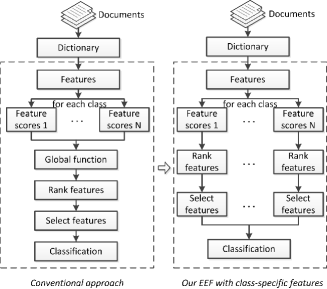
Figure 1: The flow chart of our EEF classifier with class-specific features for text categorization (right), compared with the conventional approach (left).

III-A PDF Construction

In MNB, the features (word occurrences) of each class satisfy a specific multinomial distribution. Let $\mathbf{x}\in\mathcal{R}^{D}$ be the raw feature transformed from the document, and then for each class $c_{i}$, $i=1,2,\cdots,N$, we have a multinomial distribution $p(\mathbf{x}|c_{i})$ with $D$ parameters (cell probabilities): $[p_{i,1},\cdots,p_{i,D}]$. The likelihood of observing a document $\mathbf{x}$ in class $c_{i}$ conditioned on its document length $l$ is given by:

$$p(\mathbf{x}|c_{i},l)=\frac{l!}{x_{1}!x_{2}!\cdots x_{D}!}\prod_{k=1}^{D-1}p_{i,k}^{x_{k}}p_{i,D}^{x_{D}}$$ (8)

where $\sum_{k=1}^{D}p_{i,k}=1$ and $\sum_{k=1}^{D}x_{k}=l$.

Suppose that the feature selection will select $K$ out of $D$ features. Denote $\mathbf{z}_{i}$ as the feature vector in class $c_{i}$ and $\mathbf{I}_{i}=[n^{i}_{1},\cdots,n^{i}_{K}]$ as the corresponding feature indexes in $\mathbf{x}$ such that $z_{ik}=x_{n^{i}_{k}}$. Note that the marginal distribution $p(\mathbf{z}_{i}|c_{i})$ still satisfies a multinomial distribution, but with $K+1$ elements. The $(K+1)$-st feature is the combination of all other features in $\mathbf{x}$ except for the $K$ selected features, and the multinomial distribution $p(\mathbf{z}_{i}|c_{i})$ has $K+1$ cells: $[p^{{}^{\prime}}_{i,1},\cdots,p^{{}^{\prime}}_{i,K},p^{{}^{\prime}}_{i,K+1}]$ where $p^{{}^{\prime}}_{i,k}=p_{i,n^{i}_{k}}$, $k=1,2,\cdots,K$, and $p^{{}^{\prime}}_{i,K+1}=1-\sum_{k=1}^{K}p^{{}^{\prime}}_{i,k}$.

We denote class $c_{0}$ as the reference class which consists of all given training data so that the reference distribution $p(\mathbf{x}|c_{0})$ still satisfies a multinomial distribution with $D$ parameters: $[p_{0,1},\cdots,p_{0,D}]$, each of which can be written as:

$$p_{0,k}=\sum_{i=1}^{N}p_{i,k}p(c_{i})\qquad k=1,2,\cdots,D$$ (9)

Using the general construction form in Eq. (3), we construct the PDF $p(\mathbf{x}|c_{i})$ for class $c_{i}$, $i=1,2,\cdots,N$ as follows:

$$p(\mathbf{x}|c_{i},l;\theta_{i})=\exp\left[\theta_{i}\sum_{k=1}^{K}z_{ik}\beta_{ik}-K_{1}(\theta_{i},l)+\ln p(\mathbf{x}|c_{0})\right]$$ (10)

where

$$K_{1}(\theta_{i},l)=l\ln\left(\sum_{k=1}^{K}p^{{}^{\prime}}_{0,k}\exp(\theta_{i}\beta_{ik})+\left(1-\sum_{k=1}^{K}p^{{}^{\prime}}_{0,k}\right)\right)$$ (11)

and

$$\beta_{ik}=\ln\frac{p^{{}^{\prime}}_{i,k}}{p^{{}^{\prime}}_{0,k}}-\ln\frac{p^{{}^{\prime}}_{i,K+1}}{p^{{}^{\prime}}_{0,K+1}}$$ (12)

Note that we obtain a closed form solution of the PDF construction in the original high-dimensional space of $\mathbf{x}$ as shown in Eq. (10) to Eq. (12). The detailed derivation is provided in our Supplemental Material.

Given a $N$-class training data set $\mathcal{X}=\mathcal{X}_{1}\cup\mathcal{X}_{2}\cup\cdots\cup\mathcal{X}_{N}$, each class consists of $M_{i}$ documents $\mathcal{X}_{i}=\{\mathbf{x}_{1},\mathbf{x}_{2},\cdots,\mathbf{x}_{M_{i}}\}$, and each document $\mathbf{x}_{m}$ has a length of $l_{m}=\sum_{k=1}^{D}x_{mk}$, where $x_{mk}$ is the $k$-th element in $\mathbf{x}_{m}$. We use the MLE to estimate the optimal embedding parameter, which is given by:

$$\theta^{*}_{i} =\operatorname*{arg\,max}_{\theta_{i}\in\Theta}\theta_{i}\sum_{k=1}^{K}\bar{z}_{ik}\beta_{ik}-K_{1}(\theta_{i},\bar{l})$$ (13)

where $\bar{z}_{ik}$ and $\bar{l}$ are the average of word occurrences for the $k$-th selected feature and the average of the document length over the training set $\mathcal{X}_{i}$ of class $c_{i}$, respectively. Although it is difficult to find an analytic solution of $\theta^{*}_{i}$, it can be easily found using convex optimization techniques since the objective function is a concave function with respect to $\theta_{i}$.

IV Experimental Results and Analysis

We use two real-life data sets: Reuters-10 and Reuters-20, to evaluate the performance of our proposed approach for text categorization. Both Reuters-10 and Reuters-20 data sets are the subsets of ModApte version of Reuters collection which consists of 8,293 documents with 65 classes (topics). More specifically, the data set of Reuters-10 and Reuters-20 consists of documents from the first 10 and 20 classes, respectively.

In these two data sets, we have an original feature size of $18,933$. To reduce the feature size, we apply the IG metric [19] to evaluate the feature importance. For each class $c_{i}$, the score of the $k$-th feature is calculated as follows:

(14)

where $t_{k}$ indicates the $k$-th term appears in the document, and $\bar{t}_{k}$ indicates it does not. It is shown that $IG(t_{k},c_{i})$ is a class-specific feature score. In conventional approaches, a global function, e.g., sum or average, is used to calculate class-independent feature scores for feature ranking, as shown in Fig. 1. However, the class-specific feature based classifiers rank the feature of each class with the score $IG(t_{k},c_{i})$ in Eq. (14), and use the class-specific features for classification.

We compare our EEF class-specific MNB classifier with three other state-of-the-art classifiers: MNB classifier [21], support vector machine (SVM) [22][23], and PPT class-specific MNB classifier [8]. While the first two are commonly used in text categorization with class-independent features, the last one and our classifier use class-specific features for classification. In PPT class-specific MNB classifier, we use the same reference hypothesis given by Eq. (9) and class-specific features given by Eq. (14) as used in EEF, and make the classification decision with the following rule:

$$c^{*}=\operatorname*{arg\,max}_{i=\{1,2,\cdots,N\}}\sum_{k=1}^{K+1}z_{ik}\ln\frac{p^{{}^{\prime}}_{i,k}}{p^{{}^{\prime}}_{0,k}}+\ln p(c_{i})$$ (15)

We report the classification results on the data sets of Reuters-10 and Reuters-20 in Fig. 2 and Fig. 3, respectively, where the feature size ranges from 100 to 2000. It can be shown that our EEF class-specific MNB classifier outperforms other the three methods. For the Reuters-10 data set, the two class-specific feature based MNB classifiers greatly improve the accuracy when the feature size is small. When the feature size increases, our EEF class-specific MNB shows promising performance improvement with a large margin compared to the others. For the Reuters-20 data set, it is seen that our EEF class-specific MNB consistently performs better than the others.

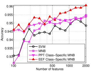
Figure 2: Classification results on Reuters-10.

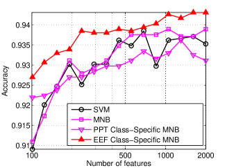
Figure 3: Classification results on Reuters-20.

V Conclusion and Future Work

In this letter, we introduced a new PDF construction method based on EEF to convert the feature PDF to the raw data PDF. With the constructed PDF on raw data, a Bayesian classifier with class-specific features is derived. As a case study, we applied the proposed EEF classifier for text categorization. The superior performance demonstrates the effectiveness of our proposed approach and indicates its wide potential application to machine learning and signal processing. In our future work, we will continue to explore its potential for various practical problems which might require different and complex reference distributions. Particularly, we are interested in applying sampling-based approaches to address the issue that the constructed distribution has no closed form for a complex reference distribution.

References

- [1] R. O. Duda, P. E. Hart, and D. G. Stork, Pattern classification. John Wiley & Sons, 2012.
- [2] C. M. Bishop, Pattern recognition and machine learning. Springer, 2006.
- [3] B. Tang and H. He, “ENN: Extended nearest neighbor method for pattern recognition [research frontier],” IEEE Computational Intelligence Magazine, vol. 10, no. 3, pp. 52–60, 2015.
- [4] B. Moghaddam and A. Pentland, “Probabilistic visual learning for object representation,” IEEE Transactions on Pattern Analysis and Machine Intelligence, vol. 19, no. 7, pp. 696–710, 1997.
- [5] B. Moghaddam, T. Jebara, and A. Pentland, “Bayesian face recognition,” Pattern Recognition, vol. 33, no. 11, pp. 1771–1782, 2000.
- [6] W. H. Wong and L. Ma, “Optional pólya tree and bayesian inference,” The Annals of Statistics, vol. 38, no. 3, pp. 1433–1459, 2010.
- [7] L. Lu, H. Jiang, and W. H. Wong, “Multivariate density estimation by bayesian sequential partitioning,” Journal of the American Statistical Association, vol. 108, no. 504, pp. 1402–1410, 2013.
- [8] P. M. Baggenstoss, “Class-specific classifier: avoiding the curse of dimensionality,” IEEE Aerospace and Electronic Systems Magazine, vol. 19, no. 1, pp. 37–52, 2004.
- [9] B. Tang, H. He, P. Baggenstoss, and S. Kay, “A Bayesian classification approach using class-specific features for text categorization,” IEEE Transactions on Knowledge and Data Engineering, vol. PP, no. 99, pp. 1–1, 2016.
- [10] R. Rifkin and A. Klautau, “In defense of one-vs-all classification,” The Journal of Machine Learning Research, vol. 5, pp. 101–141, 2004.
- [11] S. Kumar, J. Ghosh, and M. Crawford, “A hierarchical multiclassifier system for hyperspectral data analysis,” in Multiple Classifier Systems, 2000, pp. 270–279.
- [12] G. De Lannoy, D. François, and M. Verleysen, “Class-specific feature selection for one-against-all multiclass svms,” in European Symposium on Artificial Neural Networks, 2011, pp. 269–274.
- [13] S. Kay, “Exponentially embedded families-new approaches to model order estimation,” IEEE Transactions on Aerospace and Electronic Systems, vol. 41, no. 1, pp. 333–345, 2005.
- [14] P. Baggenstoss, “A maximum entropy framework for feature inversion and a new class of spectral estimators,” IEEE Transactions on Signal Processing, vol. 63, no. 11, 2015.
- [15] S. Kay, Q. Ding, B. Tang, and H. He, “Probability density function estimation using the EEF with application to subset/feature selection,” IEEE Transactions on Signal Processing, vol. 64, no. 3, pp. 641–651, 2016.
- [16] S. Kullback, Information theory and statistics. Courier Corporation, 1997.
- [17] S. Kay, Q. Ding, B. Tang, and H. He, “Probability density function estimation using the EEF with application to subset/feature selection,” IEEE Transactions on Signal Processing, vol. 64, no. 3, pp. 641–651, 2016.
- [18] B. Tang, H. He, Q. Ding, and S. Kay, “A parametric classification rule based on the exponentially embedded family,” IEEE Transactions on Neural Networks and Learning Systems, vol. 26, no. 2, pp. 367–377, 2015.
- [19] Y. Yang and J. O. Pedersen, “A comparative study on feature selection in text categorization,” in International Conference on Machine Learning, vol. 97, 1997, pp. 412–420.
- [20] B. Tang, S. Kay, and H. He, “Toward optimal feature selection in naive bayes for text categorization,” IEEE Transactions on Knowledge and Data Engineering, vol. PP, no. 99, pp. 1–1, 2016.
- [21] D. D. Lewis, “Naive (Bayes) at forty: The independence assumption in information retrieval,” in European Conference on Machine Learning, 1998, pp. 4–15.
- [22] C. Cortes and V. Vapnik, “Support-vector networks,” Machine learning, vol. 20, no. 3, pp. 273–297, 1995.
- [23] T. Joachims, Text categorization with support vector machines: Learning with many relevant features. Springer, 1998.