Computing bulk and shear viscosities from simulations of fluids with dissipative and stochastic interactions

Abstract

Exact values for bulk and shear viscosity are important to characterize a fluid and they are a necessary input for a continuum description. Here we present two novel methods to compute bulk viscosities by non-equilibrium molecular dynamics (NEMD) simulations of steady-state systems with periodic boundary conditions – one based on frequent particle displacements and one based on the application of external bulk forces with an inhomogeneous force profile.

In equilibrium simulations, viscosities can be determined from the stress tensor fluctuations via Green-Kubo relations; however, the correct incorporation of random and dissipative forces is not obvious. We discuss different expressions proposed in the literature and test them at the example of a dissipative particle dynamics (DPD) fluid.

I Introduction

To describe the flow of an isotropic and compressible Newtonian fluid on a continuum level, it is necessary to have precise values of both shear viscosity $\eta$ and bulk viscosity $\zeta$. In a Newtonian fluid, the shear viscosity $\eta$ relates a shear flow $\partial_{z}u_{x}$ to the off-diagonal component $\sigma_{xz}$ of the stress tensor and is thus a measure for the resistance of a fluid element against deformation of shape. Similarly, the bulk viscosity $\zeta$ relates a divergence in the flow field $\partial_{\alpha}u_{\alpha}$ to the trace of the stress tensor $\operatorname{Tr}\sigma$ and is thus a measure for the resistance of a fluid element against deformation of volume. For many flows only shear viscosity is of interest. However, bulk viscosity can play an important role for the Brownian motion of a large particle (e.g. a colloid) or especially for shock wave problems (e.g. damping of a sound wave). In fact shockwave problems are exactly the systems chosen experimentally to determine the bulk viscosity schmidt .

There exist two different ways to determine transport coefficients like shear and bulk viscosity of a fluid using molecular dynamics (MD). One can create a non-equilibrium state and calculate the transport coefficients using direct measurements (force, stress or flow measurements) ashurst . We will refer to this as non-equilibrium molecular dynamics (NEMD). Alternatively, equilibrium fluctuations are evaluated to determine transport coefficients using Green-Kubo greenkubo or Einstein-Helfand relations helfand .

In NEMD, it is favorable to simulate a non-equilibrium steady-state with time-independent statistical properties. This is easily possible in the case of steady-state shear flow: One can use boundary-driven shear flow schmid1 , Lees-Edwards boundary conditions leesedwards , force-driven Poiseuille flow poiseuille or momentum interchange plathe . All these methods have been used to determine the shear viscosity $\eta$ of fluids. However, creating a steady-state divergent flow field to measure the bulk viscosity $\zeta$ is much more complicated. As mentioned above, the bulk viscosity is related to the deformation of the volume of a fluid element and thus to a change of the local thermodynamic state of the system. This is the reason why it is difficult to measure the bulk viscosity in a steady-state experiment hoover1 . To the best knowledge of the authors, the only NEMD calculations of the bulk viscosity use either cyclic compression hoover1 ; hoover2 or the relaxation of an instantaneous distortion heyes ; ciccotti . The methods used in these studies cannot be applied to systems with stochastic dynamics – either because they are explicitly designed for Hamiltonian systems hoover1 ; hoover2 ; ciccotti , or, in the case of Ref. heyes , because they cannot be used to determine the instantaneous contribution of the random force to the viscosity (as already mentioned in heyes ) due to the finite time step in MD simulations. In addition to the above mentioned calculations, there have been extensive NEMD studies of the elongationaly viscosity using the so called SLLOD equation of motion elo1 ; elo2 ; elo3 . This boundary-driven NEMD method does not rely on a Hamiltonian dynamics and it should be possible to generalize it to stochastic equations of motion. However, in order to calculate the bulk viscosity, it will be necessary to choose a vanishing strain rate in order to minimize the change of volume. Therefore, all these methods depend on a perturbation parameter $\epsilon$ that has to be chosen very small to get reliable results, hence they can only be used in the linear response regime.

In that regime, using Green-Kubo or Einstein-Helfand relations is an attractive alternative to NEMD methods. The great advantage is that one can evaluate transport coefficients without having to create a non-equilibrium state. In conservative systems, both relations are well-understood and often used. However, the correct way to account for random and dissipative forces is less clear. In 1995 Español espanol suggested a generic Green-Kubo form

$$\mu=\frac{V}{k_{\text{B}}T}\int_{0}^{\infty}dt\left\langle I^{C}(0)I^{C}(t)+I^{D}(0)I^{D}(t)\right\rangle_{0},$$ (1)

which depends on the conservative and dissipative projected momentum currents $I^{C}(t)$ and $I^{D}(t)$, respectively. “Generic” means, that the equation is not restricted to a specific viscosity. In Sec. III we will identify the projected momentum currents $I(t)$ to find practical Green-Kubo relations for the shear viscosity $\eta$ and the bulk viscosity $\zeta$. The formula implies that the random force has no direct contribution and the total viscosity is just a summation of the conservative and the dissipative contribution. More recently, Español and Vázquez espanol2002 and later Ernst and Brito ernst suggested another generic Green-Kubo form,

$$\mu=\mu_{\infty}+\frac{V}{k_{\text{B}}T}\int_{0}^{\infty}dt\left\langle(I_{-}e^{t\mathcal{L}}I_{+}\right\rangle_{0},$$ (2)

where the instantaneous viscosity $\mu_{\infty}$ denotes a contribution of stochastic forces. The time evolution is defined by the pseuodstreaming operator $e^{t\mathcal{L}}$ and $I_{\pm}=I^{C}\pm I^{D}$ (details in Sec. III and Ref. ernst ). This expression explicitly accounts for the fact that the dissipative force is not invariant under time reversal symmetry. To our best knowledge, none of these formulae have been verified by simulations in the presence of random and dissipative forces to this date.

Recently Español espanol2009 also presented a generalized Einstein-Helfand form that can be used if the underlying dynamics is dissipative and stochastic. It could be shown that both relations should give the same result. In the present work we focus on generalized Green-Kubo expressions that have the useful advantage of separating the stochastic contribution and should therefore give better statistics. In the future, it will also be interesting to test Einstein-Helfand relations in the presence of stochastic and dissipative interactions.

The purpose of the present work is two-fold. First, we propose two novel NEMD techniques to measure the bulk viscosity $\zeta$ from fluid simulations of steady-state systems with periodic boundary conditions. One, denoted ”particle transfer method”, creates a divergent flow field by manually displacing particles. This method is most efficient in systems of particles interacting by soft potentials. The other, denoted ”force driven method”, makes use of a spatially varying body force and a non-zero center of mass velocity and can be used in a wider range of molecular dynamics simulations.

Second, we test the Green-Kubo relations (1) and (2) using the example of a dissipative particle dynamics (DPD) fluid and compare the resulting values with the results from NEMD simulations.

Our paper is organized as follows. In Sec. II, we present our new NEMD methods for determining bulk viscosities from fluid simulations. In Sec. III, we briefly introduce the different Green-Kubo relations for the shear and bulk viscosity. In Sec. IV, we present simulation results for DPD fluids and compare the values of the viscosity parameters obtained with different methods. We summarize and conclude in Sec. V.

II NEMD

In this section we present the NEMD methods for calculating viscosity parameters from fluid simulations. First we review the momentum interchange method to create a steady-state shear flow that was introduced by Müller-Plathe plathe . Then we introduce our novel techniques to create a steady-state divergence of the flow field. The last section explains how to evaluate the local stress tensor to determine precise values of the viscosities. The methods are illustrated by the example of DPD simulations of fluids without conservative interactions.

In DPD the particles are interacting via dissipative and random pair forces, which are constructed in a way that the total momentum is conserved dpd . Both forces are connected via fluctuation dissipation theorems such that a proper canonical distribution is reached at equilibrium espanoldpd . Therefore DPD is a Galilean invariant thermostat and can be used to study hydrodynamics. In fact, Marsh et al. marsh showed that DPD fulfills the hydrodynamic equations (Navier-Stokes equation) and calculated theoretical values for transport coefficients.

The DPD equations of motion can be written as stochastic differential equations espanoldpd

$$\text{d}\mathbf{r}_{i} = \frac{\mathbf{p}_{i}}{m}\text{d}t$$ (3)

$$\text{d}\mathbf{p}_{i} = \sum\limits_{j\neq i}-\gamma\omega_{\text{D}}(\mathbf{r}_{ij})(\mathbf{e}_{ij}\cdot\mathbf{v}_{ij})\mathbf{e}_{ij}\text{d}t+\sum\limits_{j\neq i}\sigma\omega_{\text{R}}(\mathbf{r}_{ij})\mathbf{e}_{ij}\text{d}W_{ij}$$

with the velocity difference $\mathbf{v}_{ij}=\mathbf{v}_{i}-\mathbf{v}_{j}$, the distance $\mathbf{r}_{ij}=\mathbf{r}_{i}-\mathbf{r}_{j}$ and the fluctuation dissipation theorems $\sigma=\sqrt{2k_{\text{B}}T\gamma}$ and $\omega_{\text{D}}(r)=\omega_{\text{R}}(r)^{2}$.

In the present work, we use the weight function $\omega_{\text{R}}(r)=1-\frac{r}{r_{\text{cut}}}$. The simulation units are defined by setting $k_{B}T=1$ (energy), $r_{\text{cut}}=1$ (length) and $\tau=r_{\text{cut}}\sqrt{m/k_{B}T}=1$ (time). In these units, we choose the DPD parameter $\gamma=5$ and the time step $\Delta t=0.01$.

II.1 Steady-state shear flow

If a shear flow $\partial_{z}u_{x}$ emerges in a fluid, it will be damped due to shear viscosity $\eta$. This damping can be described by a momentum flux

$$j_{z}(p_{x})=-\eta\frac{\partial u_{x}}{\partial z}$$ (4)

which transports momentum $p_{x}$ in $-z$-direction. To maintain the shear flow it is therefore necessary to counteract the damping by enforcing a similar momentum flux in $+z$-direction.

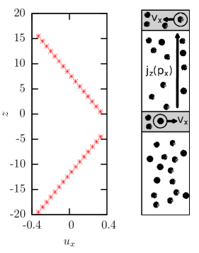
Figure 1: Momentum interchange method to generate steady-state shear flow. Right panel illustrates the idea of the method. Left panel shows the velocity profile from simulation results for a DPD fluid at density $\bar{\rho}=4$.

The idea of the momentum interchange method plathe is to produce this counter flux by swapping the momentum of particles with a certain rate. The algorithm of one interchange works as follows (see Fig. 1, right):

1. Choose the particle with the highest velocity in $+x$-direction in the middle slab

2. Choose the particle with the highest velocity in $-x$-direction in the top slab

3. Swap the momentum of these two particles

The shear rate $\dot{\gamma}=\partial_{z}u_{x}$ will depend on the rate of these momentum interchange steps and the velocity profile will be linear in good approximation if the interchange rate is not too large (see Fig. 1, left).

II.2 Steady-state divergent flow

Unfortunately, the momentum interchange method cannot be used for creating steady-state divergent flow (with gradient $\partial_{x}u_{x}$). This is because the transported momentum $p_{x}$ and the direction of flux $j_{x}(p_{x})$ are no longer orthogonal. In fact, the directions of particle and momentum transport are parallel and therefore a transport of particles is necessary to maintain the steady-state. This can be achieved in two different ways: either by manually displacing particles or by imposing a global flow. Our two methods of generating steady-state divergent flow are based on these two types of mass transport.

The methods can be motivated theoretically by solving the mass and momentum continuity equations with appropriate source terms. The local conservation of mass on a continuum level with source term reads:

$$\partial_{t}\rho+\nabla\cdot(\rho\mathbf{u})=Q_{\rho}(\mathbf{r})$$ (5)

with density $\rho(\mathbf{r},t)$, velocity field $\mathbf{u}(\mathbf{r},t)$ and mass source term $Q_{\rho}(\mathbf{r})$. Similarly one can write down the local conservation of momentum:

$$\partial_{t}(\rho\mathbf{u})+\nabla(\rho\mathbf{u}\otimes\mathbf{u})+\nabla\sigma^{\text{N}}=Q_{\rho}(\mathbf{r})\mathbf{u}+\mathbf{f}(\mathbf{r})$$ (6)

with the external force field $\mathbf{f}(\mathbf{r})$ and the constitutive relation hansen :

$${\sigma}^{\text{N}}(\mathbf{r},t)=p\mathbf{I}+\left(\frac{2}{3}\eta-\zeta\right)\nabla\cdot\mathbf{u}\mathbf{I}-\eta\left(\nabla\mathbf{u}+\nabla\mathbf{u}^{T}\right)$$ (7)

with flow field $\mathbf{u}(\mathbf{r},t)$, pressure $p$, shear viscosity $\eta$ and bulk viscosity $\zeta$.

The external force and mass source terms can be chosen freely and allow us to manipulate the flow and density profiles. However, to conserve global mass and momentum both the mass source term $Q_{\rho}(\mathbf{r})$ and the force field $\mathbf{f}(\mathbf{r})$ must fulfill the relations:

$$\int_{V}Q_{\rho}(\mathbf{r})\text{d}\mathbf{r}=0$$

$$\int_{V}\mathbf{u}(\mathbf{r})Q_{\rho}(\mathbf{r})\text{d}\mathbf{r}+\int_{V}\mathbf{f}(\mathbf{r})\text{d}\mathbf{r}=0$$

In the following, we assume that the fluid is barotropic, i.e., there exists a unique relation $p=P(\rho)$. We are interested in stationary solutions $\partial_{t}\rho=0$ and $\partial_{t}(\rho\mathbf{u})=0$, where $\mathbf{u}=u\mathbf{e}_{x}$ exhibits a gradient in $x$-direction and profiles are constant in all other directions. Assuming that higher order derivatives of the flow field can be neglected, we obtain the following equations:

$$Q_{\rho}(x) = \partial_{x}(\rho u)$$

$$f(x) = -Q_{\rho}(x)u+P^{\prime}(\rho)\partial_{x}\rho+\partial_{x}(\rho u^{2})$$ (8)

II.2.1 Particle transfer method

In the particle transfer method, we aim at creating a velocity gradient while keeping the density profile constant, $\rho(x)=\bar{\rho}$. This leads to

$$Q_{\rho}(x) = \bar{\rho}u^{\prime}(x)$$ (9)

$$f(x) = \bar{\rho}\>u\>u^{\prime}(x)$$ (10)

To get a linear profile $u(x)=\epsilon\;\left|x\right|$, one therefore has to choose a mass source term

$$Q_{\rho}(x)=\bar{\rho}\>\epsilon\>\text{sign}(x)$$ (11)

and a force term $f(x)=\bar{\rho}x\epsilon^{2}\approx 0$ which vanishes at order ${\cal O}(\epsilon)$. These source terms can be realized by transferring particles between two halves of the box at a certain rate (see Fig. 2). The algorithm is very simple:

1. Choose a random particle in the right half of the simulation box

2. Place it at a random position in the left half of the simulation box

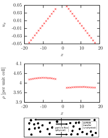
Figure 2: Particle transfer method to generate steady-state divergent flow. Bottom panel illustrates the idea of the method. Upper panels show corresponding simulation results for the velocity (top) and the density (middle) of a DPD fluid at mean density $\bar{\rho}=4$. In this method, the density is roughly constant.

This algorithm conserves momentum and – in the special case of vanishing conservative forces – also energy. As shown in Fig. 2, the resulting velocity profile is approximately linear and the density profile almost constant, in perfect agreement with the above described theoretical prediction. Therefore, this algorithm is perfectly suitable to study the bulk viscosity $\zeta$ of fluids that are interacting only via soft potentials.

However, the particle transfer method can become problematic in the presence of hard-core potentials, like the widely used Lennard-Jones potential, because particle insertion in dense fluids is difficult and usually associated with large energy penalties.

II.2.2 Force driven method

In the force driven method there is no particle transfer and hence no mass source term, $Q_{\rho}(\mathbf{r})=0$. This directly leads to $\rho u=$ const. A velocity gradient is invariably associated with a density gradient, and can only exist if the mean velocity $\bar{u}$ is nonzero.

The force density now reads

$$f(x)=-\frac{\rho}{u}(P^{\prime}(\rho)-u^{2})\>u^{\prime}(x)$$ (12)

To create a linear profile $u(x)=\bar{u}+\epsilon\>\left|x\right|$, one therefore has to apply an external force

$$f(x)=-\epsilon\>C\>\text{sign}(x)+{\cal O}(\epsilon^{2}),$$ (13)

where the constant is given by $C=\left(P^{\prime}(\bar{\rho})\>\bar{\rho}/\bar{u}-\bar{\rho}\>\bar{u}\right)$.
These equations explain how to create a linear velocity profile in the absence of a mass source term: One has to create a steady-state particle flow in the presence of periodic boundary conditions by imposing a non-zero center of mass velocity. To create a divergent flow field, one has to combine this global background flow with an external force acting on all particles, which changes sign between the two halves of the box (see Fig. 3).

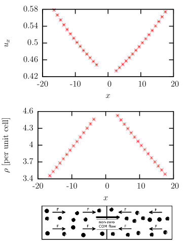
Figure 3: Force-driven method to generate steady-state divergent flow. Bottom panel illustrates the idea of the method. Upper panels show corresponding simulation results for the velocity (top) and the density (middle) of a DPD fluid at mean density $\bar{\rho}=4$. In this method, the density varies spatially.

This method has the great advantage that one does not have to manually change the position of particles. It can thus be used in combination with hard-core potentials. It is also physically more ”realistic” since it only requires an external force and a non-zero flow velocity. Therefore, the basic idea may be applicable in experiments.

The main disadvantage of this technique is that the gradient in the flow field is unavoidably associated with a density gradient. This is a problem because the bulk viscosity strongly depends on the density. One can reduce the problem by applying a very small force. However, very long simulations are then necessary to obtain sufficiently good statistics. The solution used in this work is to calculate a bulk viscosity $\zeta$ for every bin in the simulation box and associate it to the density in the respective box. In this way one obtains many data points for various densities that can be used to determine not only the bulk viscosity for a constant density but also the density dependence (see Sec. IV.2).

II.3 Local stress tensor

We calculate the viscosity by direct evaluation of the local stress tensor using both Newton’s constitutive relation and a localized Irving-Kirkwood formula. This has the great advantage that one can decouple the problems of creating a steady-state flow and calculating viscosities. When using this method it is also possible to distinguish between the dissipative and the conservative contribution to the viscosity.

II.3.1 Newton’s constitutive relation

The local stress tensor of an isotropic, compressible Newtonian fluid can be calculated using Newton’s constitutive relation (see Eq. (7)).

It can be evaluated in a particle simulation by dividing the simulation box into bins and calculating the flow field (mean velocity of all particles) in each bin. The errors due to discretization are small because of the linearity of the observed flow profiles.

II.3.2 Irving-Kirkwood formula

In a particle simulation the global stress tensor can also be calculated using the Irving-Kirkwood formula irving :

$$\sigma^{\text{IK}}_{\alpha\beta}=\left\langle\sigma^{C}_{\alpha\beta}(t)+\sigma^{D}_{\alpha\beta}(t)+\sigma^{R}_{\alpha\beta}(t)\right\rangle$$ (14)

$$\sigma^{C}_{\alpha\beta}(t)=\frac{1}{V}\sum\limits_{i<j}r_{ij\alpha}(t)F^{C}_{ij\beta}(t)+\frac{1}{V}\sum\limits_{i}mu_{i\alpha}(t)u_{i\beta}(t)$$

$$\sigma^{D}_{\alpha\beta}(t)=\frac{1}{V}\sum\limits_{i<j}r_{ij\alpha}(t)F^{D}_{ij\beta}(t)$$

$$\sigma^{R}_{\alpha\beta}(t)=\frac{1}{V}\sum\limits_{i<j}r_{ij\alpha}(t)F^{R}_{ij\beta}(t)$$

with distance $\mathbf{r}_{ij}=\mathbf{r}_{i}-\mathbf{r}_{j}$, conservative force $\mathbf{F}^{\text{C}}_{ij}$, dissipative force $\mathbf{F}^{\text{D}}_{ij}$ and random force $\mathbf{F}^{\text{R}}_{ij}$ between two particles. In our model system, there are no conservative forces and the kinetic contribution is equal to the conservative stress tensor. This equation can be evaluated locally in a homogeneous fluid by considering the contribution of all particles in one bin only.

II.3.3 Calculating viscosities

Evaluating the local stress tensor using the aforementioned formulae in a steady-state shear flow makes it possible to calculate the shear viscosity:

$$\eta=\frac{\sigma^{\text{IK}}_{xz}(\mathbf{r})}{\partial_{z}u_{x}(\mathbf{r})}$$ (15)

Similarly, in a steady-state divergent flow field, the bulk viscosity can be calculated via

$$\zeta=\frac{1}{3}\frac{\sigma^{\text{IK}}_{xx}(\mathbf{r})+\sigma^{\text{IK}}_{yy}(\mathbf{r})+\sigma^{\text{IK}}_{zz}(\mathbf{r})-3p}{\partial_{x}u_{x}(\mathbf{r})}$$ (16)

The procedure of calculating the bulk viscosity is demonstrated in Fig. 4 using the example of the particle transfer method (see Sec.II.2.1). Both the flow field and the stress tensor are evaluated locally and used to determine the bulk viscosity $\zeta$ in each bin. The final viscosity is calculated using the average of the viscosities.

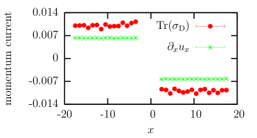
Figure 4: Profiles of divergence of the flow field and trace of the dissipative contribution to the stress tensor, obtained with the particle transfer method for a DPD fluid with density $\bar{\rho}=4.0$.

III Green-Kubo

Green-Kubo formulae use equilibrium fluctuations of the projected momentum current $I_{\alpha\beta}$ to calculate transport coefficients (see Eqs. (1) and (2)). The projected momentum current is the projection of the instantaneous momentum current fluctuation $(\sigma_{\alpha\beta}(t)-\left\langle\sigma_{\alpha\beta}\right\rangle_{0})$ (see Eq. (14)) on the irrelevant hydrodynamic variables, i.e., on the subspace of variables that is orthogonal to the slow variables of the hydrodynamic equations: energy, mass and momentum density. Here and in the following, the notation $\langle\cdot\rangle_{0}$ refers to equilibrium averages. For details see Ref. ernst1974 ).

III.1 Shear viscosity

The shear viscosity $\eta$ is related to the off-diagonal $I_{xz}$ of the projected momentum current. In this case, finding the projection is simple. The mean values $\left\langle\sigma_{xz}\right\rangle_{0}$ are zero and the momentum current is orthogonal to the relevant subspace:

$$I_{xz}=\mathcal{P}_{\perp}(\sigma_{xz}-\left\langle\sigma_{xz}\right\rangle_{0})=\sigma_{xz}$$ (17)

With this relation we can find the Green-Kubo formulae for the shear viscosity $\eta$. Equation (18) corresponds to the generic formula (1):

$$\eta=\frac{V}{k_{\text{B}}T}\int_{0}^{\infty}dt\left\langle\sigma^{C}_{xz}(0)\sigma^{C}_{xz}(t)+\sigma^{D}_{xz}(0)\sigma^{D}_{xz}(t)\right\rangle_{0}\qquad$$ (18)

and Equation (19) corresponds to the generic formula (2):

$$\eta= \eta_{\infty} +\frac{V}{k_{\text{B}}T}\int_{0}^{\infty}dt\left\langle(\sigma^{C}_{xz}(0)-\sigma^{D}_{xz}(0)(\sigma^{C}_{xz}(t)+\sigma^{D}_{xz}(t))\right\rangle_{0}$$ (19)

$$\eta_{\infty} =\frac{V}{k_{\text{B}}T}\frac{\Delta t}{2}\left\langle{\sigma^{R}_{xz}}^{2}\right\rangle_{0},$$

where the different contributions to the stress tensor $\sigma_{xz}$ are defined as in Eq. (14).

III.2 Bulk viscosity

The bulk viscosity $\zeta$ is related to the diagonal $I_{\alpha\alpha}$ of the projected momentum current. Therefore, the situation is slightly more complicated. First, the mean currents $\left\langle\sigma_{\alpha\alpha}\right\rangle_{0}$ do not vanish. Second, the momentum current fluctuations are not orthogonal to the relevant subspace. This becomes clear when considering the kinetic contribution $\sigma^{C}_{\alpha\alpha}(t)$, which is proportional to the kinetic energy and therefore depends on the energy density – a relevant variable. Therefore, the energy fluctuations enter the projected momentum current explicitly:

$$I_{\alpha\alpha}=\mathcal{P}_{\perp}(\sigma_{\alpha\alpha}-\left\langle\sigma_{\alpha\alpha}\right\rangle_{0})=\sigma_{\alpha\alpha}-\left\langle\sigma_{\alpha\alpha}\right\rangle_{0}-\frac{1}{V}\frac{\partial p}{\partial e}(\mathcal{H}-\left\langle\mathcal{H}\right\rangle_{0})$$ (20)

with the average energy density $e=V^{-1}\left\langle\mathcal{H}\right\rangle_{0}$.
This leads to the projected momentum currents:

$$I_{\zeta}^{C}(t) = \sum_{\alpha}\left[\sigma^{C}_{\alpha\alpha}(t)-\left\langle\sigma^{C}_{\alpha\alpha}\right\rangle_{0}-\frac{1}{V}\frac{\partial p}{\partial e}(\mathcal{H}(t)-\left\langle\mathcal{H}\right\rangle_{0})\right]$$

$$I_{\zeta}^{D}(t) = \sum_{\alpha}\left[\sigma^{D}_{\alpha\alpha}(t)-\left\langle\sigma^{D}_{\alpha\alpha}\right\rangle_{0}\right]$$ (21)

With Eqs. (20), (III.2) and the considerations above, we are able to find the Green-Kubo formulae for the bulk viscosity $\zeta$. Equation (22) corresponds to the generic formula (1):

$$\zeta=\frac{V}{k_{\text{B}}T}\int_{0}^{\infty}dt\left\langle I_{\zeta}^{C}(0)I_{\zeta}^{C}(t)+I_{\zeta}^{D}(0)I_{\zeta}^{D}(t)\right\rangle_{0}\qquad$$ (22)

And Equation (23) corresponds to the generic formula (2):

$$\zeta= \zeta_{\infty} +\frac{V}{k_{\text{B}}T}\int_{0}^{\infty}dt\left\langle(I_{\zeta}^{C}(0)-I_{\zeta}^{D}(0))(I_{\zeta}^{C}(t)+I_{\zeta}^{D}(t))\right\rangle_{0}$$ (23)

$$\zeta_{\infty} =\frac{V}{k_{\text{B}}T}\frac{\Delta t}{18}\left\langle[\sum_{\alpha}\sigma^{R}_{\alpha\alpha}]^{2}\right\rangle_{0}$$

For an ideal gas (like our DPD fluid without conservative forces) it is easy to calculate the thermodynamic relation:

$$\frac{\partial p}{\partial e}=\frac{2}{3}$$ (24)

This leads to a vanishing conservative contribution to the projected momentum current $I_{\zeta}^{C}(t)=0$ .

IV Results

IV.1 Shear viscosity

In this section, we focus on the test of the Green-Kubo formulae introduced in Sec. III.

For comparison we first calculated the shear viscosity using different NEMD methods. The first two are based on the momentum interchange method (see Sec. II.1), where we computed the viscosity both by measuring the momentum flux (as suggested in Ref. plathe ) and by comparing local stress tensors (as discussed in Sec. II.3.3). As a third, independent NEMD approach, we also performed simulations of confined slabs with tunable-slip boundaries at the walls (see Ref. schmid1 ) and determined the viscosity by evaluating the force on the boundary that is needed to maintain the shear flow.

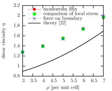
Figure 5: Results for the shear viscosity $\eta$ for different densities using several NEMD techniques (see Sec. IV.1) and theoretical prediction.

As shown in Fig. 5, all these different NEMD methods give the same result for the shear viscosity. We therefore have a reliable dataset to test the Green-Kubo formulae. When comparing the results to the theoretical prediction (see marsh ) one can observe a constant offset of about 0.30. Hence, the $\rho^{2}$ dependence of the dissipative contribution $\eta_{\text{D}}$ matches quite well but the kinetic contribution $\eta_{\text{C}}$ seems to be underestimated by the theory. This interpretation is confirmed if we compare separately the dissipative and conservative contributions to the theoretical expression for the shear viscosity with the corresponding NEMD results using the local stress tensor. This discrepancy between simulations and theory has already been noticed by Marsh et. al in Ref. marsh .

The Green-Kubo relations were evaluated by calculating the stress autocorrelation functions with resolution $\Delta t$. Then the correlation functions were integrated numerically using the trapezoidal rule, until the correlations reached about 1 % of their initial values. The tail was incorporated by fitting the correlation function with the power law $c(t)=At^{-B}$ and integrating it analytically.

The results of these calculations can be found in Fig. 6. We used the momentum flux values for comparison with NEMD because they have the smallest statistical error.

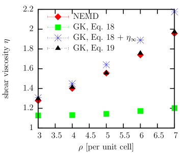
Figure 6: Results for the shear viscosity $\eta$ for different densities using different Green-Kubo relations. The values are compared to the NEMD results from the momentum flux technique.

The results obtained with the Green-Kubo formula (19) are in excellent agreement with the NEMD results. Good agreement is also obtained with Eq. (18) for small densities, if the instantaneous viscosity $\eta_{\infty}$ is added. The reason is that the dissipative contribution to the viscosity is small at small densities. However, at large densities, the results obtained with Eq. (18) and the NEMD results significantly differ from each other.

IV.2 Bulk viscosity

The bulk viscosity was determined using the NEMD method described in Sec. II.2 and the Green-Kubo formula (23). The results are also compared to theory marsh .

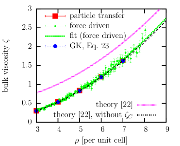
Figure 7: Results for the bulk viscosity $\zeta$ for different densities using NEMD and Green-Kubo relations.

As in the case of the shear viscosity the agreement between the NEMD results and the Green-Kubo relations is excellent. However, the simulations are not consistent with the theoretical prediction in Ref. marsh . As shown in Fig. 7 the discrepancy between theory and simulation can be resolved by neglecting the kinetic contribution in the theoretical prediction.

We rationalize the discrepancy between simulation and theory as follows: The kinetic contribution in the theoretical prediction for the stress tensor reflects the contribution of energy fluctuations to the pressure $p$, and not to the viscous stress tensor. Hence it should not be associated with the bulk viscosity $\zeta$.

In the projected momentum current Eq. (20), the corresponding term had to be subtracted. Likewise, it should also be subtracted in the Chapman-Enskog expansion of the theoretical prediction marsh .

V Summary and outlook

In the present paper, we have proposed two different techniques to create a divergence in the flow field of a homogeneous fluid. Both methods use very different mechanisms to create the flow. Therefore, one can choose the method most suited for the system to investigate. It will be interesting to test these techniques for other systems (e.g. an isothermal Lennard-Jones system) with high densities and hard-core potentials.

Furthermore, we have proposed a way to calculate the viscosities by comparing different expressions for the local stress tensor (Sec. II.3), which is independent of the methods used to create a non-equilibrium steady-state and can therefore be applied generally in the presence of arbitrary steady-state flows. The disadvantage of this method is the necessity to calculate the local stress tensor. While this task is simple in the presence of short-range two-body potentials in a homogeneous confinement, it can be more challenging for more complicated systems (e.g. in the presence of charges).

The NEMD methods proposed here can be used to compute bulk viscosities both in Hamiltonian systems and in dissipative systems (with local momentum conservation). Moreover, they are not restricted to the linear response regime, but can also be used to study nonlinear behavior.

Using NEMD simulations to determine the shear viscosity $\eta$, we were also able to test Green-Kubo relations in the presence of random and dissipative forces. The results clearly support the validity of the generic expression Eq. (2), which includes the contribution of stochastic forces and accounts for the lack of time reversal symmetry in the dissipative force.

References

- (1) A.J. Schmidt et al., Appl. Phys. Lett. 92, 244107 (2008)
- (2) W.T. Ashurst and W.G. Hoover, Phys. Rev. Lett. 31, 206 (1973)
- (3) M.S. Green, J. Chem. Phys. 22, 398 (1954); R. Kubo, J. Phys. Soc. Jpn. 12, 570 (1957)
- (4) E. Helfand, Phys. Rev. E 119, 1 (1960)
- (5) J. Zhou, J. Smiatek, E.S. Asmolov, O.I. Vinogradova and F. Schmid, Springer HPC ’14, 19 (2014)
- (6) A.W. Lees and S.F. Edwards, J. Phys. C 5, 1921 (1972)
- (7) J. Backer, C. Lowe, H. Hoefsloot and P. Iedema, J. Chem. Phys. 122, 154503 (2005)
- (8) Florian Müller-Plathe, Phys. Rev. E 59, 4894 (1998)
- (9) W.G. Hoover, A.J.C. Ladd, R.B. Hickman and B.L. Holian, Phys. Rev. A 21, 1756 (1980)
- (10) W.G. Hoover, D.J. Evans, R.B. Hickman, A.J.C. Ladd, W.T. Ashurst and B. Moran, Phys. Rev. A 22, 1690 (1980)
- (11) D. Heyes, J. Chem. Soc., Faraday Trans. 2 80, 1363 (1984)
- (12) P.L. Palla, C. Pierleoni and G. Ciccotti, Phys. Rev. E 78, 021204 (2008)
- (13) B.D. Todd and P.J. Daivis, J. Chem Phys. 107, 1617 (1997)
- (14) B.D. Todd and P.J. Daivis, Com. Phys. Comm. 177, 191 (1999)
- (15) A. Baranyai and P.T. Cummings, J. Chem. Phys. 110, 42 (1999)
- (16) P. Español, Phys. Rev. E 52, 1734 (1995)
- (17) P. Español and F. Vázquez, Phil. Trans. R. Soc. A 360, 383 (2002)
- (18) M.H. Ernst and R. Brito, Europhys. Lett. 73, 183 (2006)
- (19) P. Español, Phys. Rev. E 80, 061113 (2009)
- (20) P.J. Hoogerbrugge and J.M.V.A. Koelman, Europhys. Lett. 19, 155 (1992)
- (21) P. Español and P. Warren, Europhys. Lett. 30, 191 (1995)
- (22) C.A.Marsh, G. Backx and M.H. Ernst, Phys. Rev. E 56, 1676 (1997)
- (23) J.P. Hansen and I.R. McDonald, “Theory of simple liquids”, Academic Press (2006)
- (24) J.H. Irving and J.G. Kirkwood, J. Chem. Phys. 18, 817 (1950)
- (25) M.H. Ernst and J.R. Dorfman, J. Stat. Phys. 12, 311 (1974)