Near-threshold production of heavy quarks with QQbar_threshold

Abstract

We describe the QQbar_threshold library for computing the production cross section of heavy quark-antiquark pairs near threshold at electron-positron colliders. The prediction includes all presently known QCD, electroweak, Higgs, and nonresonant corrections in the combined nonrelativistic and weak-coupling expansion.

Program summary

• Program title: QQbar_threshold

• Programming language: C++, Wolfram Language.

• Computer: PC.

• Operating System: Linux, OS X.

• License: GNU GPLv3.

• RAM: 60 MB

• Disk Space: 63 MB (26 MB download)

• External Routines: Boost (http:///www.boost.org),
  GSL (http://www.gnu.org/software/gsl/).

• Nature of problem: Precision predictions for the pair-production cross section near threshold are essential in order to determine the properties of heavy quarks.

• Solution method: Formulas for all known perturbative corrections are implemented, so that QQbar_threshold provides a state-of-the-art theory prediction.

• Restrictions: Non-perturbative effects are not accounted for. This limits the applicability in the case of bottom quarks and excludes all lighter quarks. Due to the nonrelativistic approximation predictions for the cross section are only reliable near threshold.

• Running time: Typically about $5\,$ms per parameter point.

Contents

1. 1 Introduction
2. 2 Installation
   1. 2.1 Linux
   2. 2.2 OS X
3. 3 Basic usage and examples
   1. 3.1 Mathematica usage
   2. 3.2 Resonances
   3. 3.3 Cross sections
      1. 3.3.1 Grids
      2. 3.3.2 Thresholds
   4. 3.4 Basic options
   5. 3.5 Scheme conversion
   6. 3.6 Top quark width
4. 4 Structure of the cross section
   1. 4.1 Power counting
   2. 4.2 Resummation of QED effects
   3. 4.3 Nonresonant cross section
   4. 4.4 Production channels
   5. 4.5 Pole resummation
   6. 4.6 Hard matching
      1. 4.6.1 QCD and Higgs
      2. 4.6.2 Electroweak
   7. 4.7 Green functions
   8. 4.8 Potentials
   9. 4.9 Energy levels and residues
   10. 4.10 Mass schemes
5. 5 Options
6. 6 Advanced usage
   1. 6.1 Wave function at the origin
   2. 6.2 Parallelisation
      1. 6.2.1 C++
      2. 6.2.2 Mathematica
   3. 6.3 Moments for nonrelativistic sum rules
7. 7 Grid generation
   1. 7.1 Top and bottom grids
   2. 7.2 Nonresonant grids
8. A Predefined constants

1 Introduction

One of the main physics goals of envisaged high-energy electron-positron colliders is to precisely measure the properties of the top quark. It is expected that the top quark mass and width can be determined with high accuracy by measuring the shape of the top-antitop production cross section around threshold [1, 2]. Due to strong non-perturbative effects such an analysis is not possible for the lighter quarks observed at present low-energy electron-positron colliders. For bottom quarks, however, $\Upsilon$ sum rules can be used to extract the mass from moments of the pair-production cross section near threshold [3, 4, 5]. In both cases, a precise theory prediction of the cross section is indispensable.

Near the production threshold, the Coulomb interaction between the quark and the antiquark leads to a strong enhancement of the cross section, and has to be included to all orders in perturbation theory. This is achieved in the effective theory frameworks of potential nonrelativistic quantum chromodynamics (PNRQCD) [6] and velocity nonrelativistic quantum chromodynamics [7]. Corrections from strong interactions up to next-to-next-to leading order (N²LO) have been known for more than a decade [8] and are available in both formalisms. More recently, also the calculation of the third-order QCD corrections within PNRQCD has been finished [9]. Furthermore, corrections from P-wave production [10], non-resonant production [11, 12, 13, 14], Higgs effects [15, 16, 17, 18, 19], and further electroweak interactions [20, 16, 21, 22] are known. While all of these parts are available, it is non-trivial to combine all formulas consistently and evaluate the result numerically.

The QQbar_threshold library provides functions to compute the production cross section of heavy quark pairs near threshold and related quantities like S-wave binding energies and bound state residues. It is intended to be as flexible as possible, supporting a plethora of options and tunable input parameters. All of the functionality documented in this work can be accessed easily from both C++ and Wolfram Mathematica programs. In the following we give an overview of the library and its main functionality. An up-to-date comprehensive documentation can be found on https://qqbarthreshold.hepforge.org/. After a short description of the installation process in section 2, we explain the basic usage with some examples in section 3. Section 4 describes the structure of the cross section, which allows us to give a more detailed account of all optional settings in section 5. We then proceed to discuss some more advanced applications in section 6. Finally, section 7 describes the generation of auxiliary grids.

2 Installation

2.1 Linux

The easiest way to install QQbar_threshold is via the included installation script. The following software has to be available on the system:

• a compiler complying with the C++11 standard (e.g. g++ 4.8 or higher);

• cmake (http://cmake.org/);

• GSL, the GNU scientific library (http://www.gnu.org/software/gsl);

• the QCD library (included in the installation script);

• the QCD library requires odeint from the boost libraries (http://www.boost.org/).

It is recommended to run the installation script in a separate build directory, e.g. /tmp/build/. After changing to such a directory, the following code can be run in a terminal to download QQbar_threshold and install it to the directory /my/path/:

⬇

wget https://www.hepforge.org/archive/qqbarthreshold/install.tar.gz

tar xzf install.tar.gz

cd QQbar_threshold_source

./install.sh /my/path/

If /my/path/ is omitted, a default directory (usually /usr/local/) will be used.

During installation there is the opportunity to change some predefined physical constants like the W and Z masses and the default settings for some of the options discussed in section 5. A table of the default values is given in appendix A. Changing these values after installation will have no effect at best and might even lead to inconsistent results. If Mathematica is available on the system the QQbarThreshold package will also be installed automatically.

Before using the C++ library part, it may also be necessary to adjust certain environment variables. After installation to the base directory /my/path/ the following settings are recommended:

⬇

LIBRARY_PATH="/my/path/lib:$LIBRARY_PATH"

LD_LIBRARY_PATH="/my/path/lib:$LD_LIBRARY_PATH"

CPLUS_INCLUDE_PATH="/my/path/include:$CPLUS_INCLUDE_PATH"

2.2 OS X

Under OS X, QQbar_threshold can be installed like under Linux, apart from two exceptions. First, the environment variable DYLD_LIBRARY_PATH should be set in place of LD_LIBRARY_PATH. Second, typical Mathematica installations do not provide the required math executable and the QQbarThreshold Mathematica package will not be installed automatically. One way around this is to locate the WolframKernel (or MathKernel) executable included in the Mathematica installation and provide a small wrapper script. Assuming WolframKernel can be found under /Applications/Mathematica.app/Contents/MacOS/ the following shell script can be used:

⬇

#!/bin/sh

MATH_PATH=/Applications/Mathematica.app/Contents/MacOS/

DYLD_LIBRARY_PATH="$DYLD_LIBRARY_PATH:$MATH_PATH"

$MATH_PATH/WolframKernel "$@"

For the installation of the Mathematica package to work, the script file has to be in the executable path and must be named math. After installing the QQbarThreshold Mathematica package, the above script is no longer required and can be safely removed.

3 Basic usage and examples

In this section, we give a brief overview over QQbar_threshold’s main functionality and show several code examples. For the sake of a more accessible presentation we postpone the discussion of most details to later sections.

The main observables that can be computed with QQbar_threshold are the total cross section and the energy levels and residues of quarkonium bound states. The cross section is calculated in picobarn, whereas all other dimensionful quantities are given in (powers of) GeV. While the examples below demonstrate the usage of specialised C++ header files, we also provide a header QQbar_threshold.hpp which exposes all functionality offered by the QQbar_threshold library. Functions related to $t\bar{t}$ production start with the prefix ttbar_; correspondingly bbbar_ designates $b\bar{b}$ functions. All (public) parts of the library are in the QQbar_threshold namespace.

The C++ examples below have to be compiled with a reasonably recent compiler (complying with the C++11 standard) and linked to the QQbar_threshold library. For example, one could compile the first code snippet resonance.cpp with the g++ compiler (version 4.8 or higher) with the command

⬇

g++ -o resonance -std=c++11 resonance.cpp -lQQbar_threshold

and run it with

⬇

./resonance

The code for all examples will also be installed alongside with the library. Assuming again /my/path as the base directory, it can be found under /my/path/include/QQbar_threshold/examples.

3.1 Mathematica usage

While the following main text generally describes the usage in C++ programs, the C++ code examples are also followed by equivalent Mathematica code. After loading the package with Needs["QQbarThreshold‘"] an overview over the available symbols can be obtained with Names["QQbarThreshold‘*"]. QQbarThreshold follows the usual conventions for documenting symbols; e.g. Information[TTbarXSection] or ?TTbarXSection explains the TTbarXSection function and Options[TTbarXSection] shows its options and their default settings.

3.2 Resonances

QQbar_threshold can calculate the binding energy of the S-wave $Q\bar{Q}$ resonances. As a first example, we calculate the binding energy of the $\Upsilon(1S)$ resonance at leading order. The binding energy $E^{\text{RS}}_{1}$ depends on the chosen renormalisation scheme and is defined by $E^{\text{RS}}_{1}=M_{\Upsilon(1S)}-2\*m^{\text{RS}}_{b}$, where $m^{\text{RS}}_{b}$ is the bottom-quark mass in the given scheme RS, and $M_{\Upsilon(1S)}$ refers to the theoretically computed mass of the $\Upsilon(1S)$. By default, the quark masses are defined in the PS-shift scheme (cf. section 4.10). All masses and energies are in GeV, so the output implies that at leading order $E^{\text{PS}}_{1}=0.273409\,$GeV.

examples/C++/resonance.cpp

⬇

#include <iostream>

#include "QQbar_threshold/energy_levels.hpp"

int main(){

namespace QQt = QQbar_threshold;

const double mb_PS = 4.5; // bottom mass in PS scheme

double E_1 = QQt::bbbar_energy_level(

1, // principal quantum number

mb_PS, // renormalisation scale

mb_PS, // quark mass

QQt::LO // perturbative order

);

std::cout << E_1 << ’\n’;

}

examples/Mathematica/resonance.m

⬇

Needs["QQbarThreshold‘"];

With[

{mbPS = 4.5, scale = 4.5},

E1 = BBbarEnergyLevel[1, scale, mbPS, "LO"]

];

Print[E1];

The corresponding residue (see eq. (27) for a definition) can be computed in very much the same way using the bbbar_residue function in C++ or BBbarResidue in Mathematica. The calculation of the (scheme-dependent) nonrelativistic wave function at the origin is slightly more involved and are covered in section 6.1.

Higher-order corrections can be included by changing the last argument to QQt::NLO, QQt::N2LO, or QQt::N3LO ("NLO", "N2LO", or "N3LO" in Mathematica). It should be noted that at the highest order, i.e. N³LO, energy levels and residues are only implemented for the six lowest resonances. At lower orders, however, the principal quantum number can be an arbitrary positive integer.

3.3 Cross sections

One of the most interesting phenomenological applications is the threshold scan of the $t\bar{t}$ production cross section. The functions ttbar_xsection and bbbar_xsection compute the cross sections

$$\sigma_{t}(s)={} \sigma(e^{+}e^{-}\to W^{+}W^{-}b\bar{b})\,,$$ (1)

$$\sigma_{b}(s)={} \sigma(e^{+}e^{-}\to b\bar{b})\,,$$ (2)

in picobarn. The name ttbar_xsection is justified by the fact that near the $t\bar{t}$ threshold $\sigma_{t}$ is dominated by the production and subsequent decay of a $t\bar{t}$ pair near mass shell; see section 4.3 for details. Here is an example for computing the cross section at a single point at next-to-leading order for $m_{t}^{\text{PS}}(20\,\text{GeV})=168\,$GeV and a top width of $1.4\,$GeV with the result $\sigma_{t}\big{(}(340\,\text{GeV})^{2}\big{)}=0.724149\,\text{pb}$:

examples/C++/xsection_0.cpp

⬇

#include <iostream>

#include "QQbar_threshold/xsection.hpp"

int main(){

namespace QQt = QQbar_threshold;

std::cout

// QQt::ttbar_xsection(sqrt_s, {scales}, {mass, width}, order)

<< QQt::ttbar_xsection(340., {80., 350.}, {168., 1.4}, QQt::NLO)

<< ’\n’;

}

examples/Mathematica/xsection_0.m

⬇

Needs["QQbarThreshold‘"];

Print[TTbarXSection[340., {80., 350.}, {168., 1.4}, "NLO"]];

Note that in this example two scales appear. As before, the first scale is the overall renormalisation scale. The second scale is due to the separation of resonant and nonresonant contributions to the cross section (cf. section 4.3). It exclusively appears in the top cross section, all other functions only take a single scale as their argument.

3.3.1 Grids

For N²LO and N³LO corrections to the cross section, it is necessary to load a precomputed grid first. Some default grids can be found in the grids subdirectory of the installation. The generation of custom grids is explained in section 7. For convenience, the grid_directory function returns the directory containing the default grids. The following code performs a threshold scan at N³LO and prints a table of the cross sections for centre-of-mass energies between $330$ and $345\,$GeV:

examples/C++/xsection_1.cpp

⬇

#include "QQbar_threshold/load_grid.hpp"

#include "QQbar_threshold/xsection.hpp"

#include <iostream>

int main(){

namespace QQt = QQbar_threshold;

QQt::load_grid(QQt::grid_directory() + "ttbar_grid.tsv");

const double mu = 50.;

const double mu_width = 350.;

const double mt_PS = 168.;

const double width = 1.4;

for (double sqrt_s = 330.; sqrt_s < 345.; sqrt_s += 1.0) {

std::cout << sqrt_s << ’\t’

<< QQt::ttbar_xsection(

sqrt_s ,{mu, mu_width} ,{mt_PS , width}, QQt::N3LO

)

<< ’\n’;

}

}

examples/Mathematica/xsection_1.m

⬇

Needs["QQbarThreshold‘"];

LoadGrid[GridDirectory <> "ttbar_grid.tsv"];

With[

{

mu = 50.,

mtPS = 168.,

width = 1.4,

muWidth = 350.,

order = "N3LO"

},

Do[

Print[

sqrts, "\t",

TTbarXSection[sqrts, {mu, muWidth}, {mtPS, width}, order]

],

{sqrts, 330., 345., 1.}

]

];

Grids cover a specific range in the rescaled energy and width coordinates

$$\tilde{E}={} -4/(\alpha_{s}^{2}\*C_{F}^{2}\*m_{Q})\*E\,,$$ (3)

$$\tilde{\Gamma}={} -4/(\alpha_{s}^{2}\*C_{F}^{2}\*m_{Q})\*\Gamma\,,$$ (4)

where $m_{Q}$ is the pole quark mass, $E=\sqrt{s}-2\*m_{Q}$ the kinetic energy, and $C_{F}=4/3$. If the arguments of the cross section functions lead to rescaled coordinates outside the range covered by the grid an exception is thrown. In the Mathematica package an error message is displayed and the cross section function will return a symbolic LibraryFunctionError.

After loading a grid, its coordinate range can be identified as shown in the following example. For the default top grid, the range is $-10.4956\leq\tilde{E}\leq 17.0554$ and $-1.83673\leq\tilde{\Gamma}\leq-0.918367$. For the default bottom grid we would find $-37.1901\leq\tilde{E}\leq-9.29752\times 10^{-6}$ and $-9.29752\times 10^{-8}\leq\tilde{\Gamma}\leq-4.55432\times 10^{-15}$

examples/C++/grid_range.cpp

⬇

#include "QQbar_threshold/load_grid.hpp"

#include "QQbar_threshold/xsection.hpp"

#include <iostream>

int main(){

namespace QQt = QQbar_threshold;

QQt::load_grid(QQt::grid_directory() + "ttbar_grid.tsv");

auto range = QQt::grid_range();

std::cout << "Et range: (" << range.Et_min

<< ", " << range.Et_max << ")\n";

std::cout << "Gammat range: (" << range.Gammat_min

<< ", " << range.Gammat_max << ")\n";

}

examples/Mathematica/grid_range.m

⬇

Needs["QQbarThreshold‘"];

LoadGrid[GridDirectory <> "ttbar_grid.tsv"];

Print["Et range: ", {GridEtMin[], GridEtMax[]}];

Print["Gammat range: ", {GridGammatMin[], GridGammatMax[]}];

If no grid is loaded $0$ will be returned for all coordinate limits.

Note that at most one grid can be used at any given time; if a second grid is loaded it will replace the first one. Loading a grid is not thread safe, i.e. one should not try to load more than one grid in parallel. See section 6.2 for more details on parallelisation.

3.3.2 Thresholds

For convenience, there are also the functions ttbar_threshold and bbbar_thresholdto compute the naïve production threshold, which is given by twice the pole mass. In the following example, a scan around this naïve threshold is performed. The centre-of-mass energy ranges from $2\*m_{t}-3\,$GeV to $2\*m_{t}+5\,$GeV, where the pole mass $m_{t}$ is calculated from the input mass in the PS scheme.

examples/C++/xsection_2.cpp

⬇

#include <iostream>

#include "QQbar_threshold/load_grid.hpp"

#include "QQbar_threshold/xsection.hpp"

int main(){

namespace QQt = QQbar_threshold;

QQt::load_grid(QQt::grid_directory() + "ttbar_grid.tsv");

const double mu = 50.;

const double mu_width = 350.;

const double mt_PS = 168.;

const double width = 1.4;

const auto order = QQt::N3LO;

const double thr = QQt::ttbar_threshold(mu, mt_PS, order);

for(double E = -3.; E < 5.; E += 1.0){

double sqrt_s = thr + E;

std::cout << sqrt_s << ’\t’

<< QQt::ttbar_xsection(

sqrt_s, {mu, mu_width}, {mt_PS, width}, order

)

<< ’\n’;

}

}

examples/Mathematica/xsection_2.m

⬇

Needs["QQbarThreshold‘"];

LoadGrid[GridDirectory <> "ttbar_grid.tsv"];

With[

{

mu = 50.,

muWidth = 350.,

mtPS = 168.,

width = 1.4,

order = "N3LO"

},

With[

{thr = TTbarThreshold[mu, mtPS, order]},

Do[

Print[

thr + energy, "\t",

TTbarXSection[

thr + energy, {mu, muWidth}, {mtPS, width}, order

]

],

{energy, -3., 5., 1.}

]

]

];

For the case that the centre-of-mass energy is not required anywhere else in the program, the C++ threshold class allows a more concise notation. If used inside the first argument of a cross section function, it will be equivalent to a matching ttbar_threshold or bbbar_threshold function with the arguments of the surrounding cross section function. Thus, in this example the $b\bar{b}$ cross section at threshold $\sigma_{b}(4\*m_{b}^{2})=167.214\,\text{pb}$ is evaluated:

examples/C++/xsection_3.cpp

⬇

#include <iostream>

#include "QQbar_threshold/load_grid.hpp"

#include "QQbar_threshold/xsection.hpp"

#include "QQbar_threshold/threshold.hpp"

int main(){

namespace QQt = QQbar_threshold;

QQt::load_grid(QQt::grid_directory() + "bbbar_grid.tsv");

std::cout

<< bbbar_xsection(QQt::threshold()+1e-3, 4.5, 4.5, QQt::N3LO)

// equivalent to

// << QQt::bbbar_xsection(

// QQt::bbbar_threshold(4.5, 4.5, QQt::N3LO) + 1e-3,

// 4.5, 4.5, QQt::N3LO

// )

<< ’\n’;

}

In Mathematica, we can use the symbol QQbarThreshold to the same effect.

examples/Mathematica/xsection_3.m

⬇

Needs["QQbarThreshold‘"];

LoadGrid[GridDirectory <> "bbbar_grid.tsv"];

Print[BBbarXSection[QQbarThreshold + 10^-3, 4.5, 4.5, "N3LO"]];

Note that for the bottom quark the width is considered to be zero and thus the continuum cross section is discontinuous at the production threshold. In fact, the expression for the cross section directly at threshold is currently not known to N³LO and it is necessary to add a small positive offset to the energy, which was somewhat arbitrarily set to $1\,$MeV in the above examples.

3.4 Basic options

The functions provided by QQbar_threshold support a plethora of optional settings to control their behaviour. In this section we only discuss a small selection; a short summary of all options (table 1) followed by a comprehensive discussion is given in section 5. The default settings for the options are given by top_options() for top-related functions and bottom_options() for the bottom-related counterparts.

As an example let us have another look at the $t\bar{t}$ threshold scan. Here, we change the renormalisation scheme for the mass from the default PS-shift scheme to the $\overline{\text{MS}}$ scheme and discard all Standard Model corrections beyond QCD.

examples/C++/opt_0.cpp

⬇

#include <iostream>

#include "QQbar_threshold/load_grid.hpp"

#include "QQbar_threshold/xsection.hpp"

int main(){

namespace QQt = QQbar_threshold;

QQt::load_grid(QQt::grid_directory() + "ttbar_grid.tsv");

const double mu = 50.;

const double mu_width = 350.;

const double mt_MS = 160.; // mass mt(mt) in the MSbar scheme

const double width = 1.4;

QQt::options opt = QQt::top_options();

// MSbar scheme with mu_MSbar = mt_MS

opt.mass_scheme = {QQt::MSshift, mt_MS};

// turn off all non-QCD corrections

opt.beyond_QCD = QQt::SM::none;

for(double sqrt_s = 330.; sqrt_s < 345.; sqrt_s += 1.0){

std::cout << sqrt_s << ’\t’

<< QQt::ttbar_xsection(

sqrt_s, {mu, mu_width}, {mt_MS, width}, QQt::N3LO,

opt

)

<< ’\n’;

}

}

examples/Mathematica/opt_0.m

⬇

Needs["QQbarThreshold‘"];

LoadGrid[GridDirectory <> "ttbar_grid.tsv"];

With[

{

mu = 50.,

muWidth = 350.,

mtMS = 160., (* mass mt(mt) in the MSbar scheme *)

width = 1.4,

order = "N3LO"

},

Do[

Print[

sqrts, "\t",

TTbarXSection[

sqrts, {mu, muWidth}, {mtMS, width}, order,

MassScheme -> {"MSshift", mtMS},

BeyondQCD -> None

]

],

{sqrts, 330., 345., 1.}

]

];

Another useful option allows to modify the reference value for the strong coupling at the scale of the Z boson mass:

examples/C++/opt_1.cpp

⬇

#include <iostream>

#include "QQbar_threshold/load_grid.hpp"

#include "QQbar_threshold/xsection.hpp"

int main(){

namespace QQt = QQbar_threshold;

QQt::load_grid(QQt::grid_directory() + "ttbar_grid.tsv");

const double mu = 50.;

const double mu_width = 350.;

const double mt_PS = 168.;

const double width = 1.4;

QQt::options opt = QQt::top_options();

opt.alpha_s_mZ = 0.1174;

for( double sqrt_s = 330.; sqrt_s < 345.; sqrt_s += 1.0){

std::cout << sqrt_s << ’\t’

<< QQt::ttbar_xsection(

sqrt_s, {mu, mu_width}, {mt_PS, width}, QQt::N3LO,

opt

)

<< ’\n’;

}

}

examples/Mathematica/opt_1.m

⬇

Needs["QQbarThreshold‘"];

LoadGrid[GridDirectory <> "ttbar_grid.tsv"];

With[

{

mu = 50.,

muWidth = 350.,

mtPS = 168.,

width = 1.4,

order = "N3LO"

},

Do[

Print[

sqrts, "\t",

TTbarXSection[

sqrts, {mu, muWidth}, {mtPS, width}, order,

alphaSmZ -> 0.1174

]

],

{sqrts, 330., 345., 1.}

]

];

For debugging purposes it can be quite helpful to print the current option settings. The following example shows the default options for top-related functions. Note that for some options the default is signified by a physically meaningless sentinel value.

examples/C++/opt_2.cpp

⬇

#include <iostream>

#include "QQbar_threshold/parameters.hpp"

int main(){

std::cout << QQbar_threshold::top_options();

}

In the Mathematica package the current option settings if different from the default are always visible through their specification in the function call. The default settings for a given function can be inspected with Options[function].

It is also possible to inspect the settings used internally for the actual calculation:

examples/C++/opt_3.cpp

⬇

#include <iostream>

#include "QQbar_threshold/parameters.hpp"

int main(){

namespace QQt = QQbar_threshold;

const double sqrt_s = 340.;

const double mu = 50.;

const double mu_width = 350.;

const double mt_PS = 168.;

const double width = 1.4;

const auto order = QQt::N3LO;

// internal settings for top cross section

std::cout << QQt::top_internal_settings(

sqrt_s, {mu, mu_width}, {mt_PS, width}, order,

QQt::top_options()

);

// internal settings for energy levels and residues

std::cout << QQt::top_internal_settings(

mu, mt_PS, order,

QQt::top_options()

);

}

examples/Mathematica/opt_3.m

⬇

Needs["QQbarThreshold‘"];

With[

{

sqrts = 340.,

mu = 50.,

muWidth = 350.,

mtPS = 168.,

width = 1.4,

order = "N3LO"

},

Print[

TopInternalSettings[sqrts, {mu, muWidth}, {mtPS, width}, order]

];

Print[TopInternalSettings[mu, mtPS, order]];

];

Correspondingly, for bottom quarks the function bottom_internal_settings can be used. The arguments match the respective energy level, residue, or cross section function.

3.5 Scheme conversion

While the PS scheme is appropriate for the description of threshold observables, in other kinematic regions schemes like $\overline{\text{MS}}$ may be more suitable. For converting masses to the pole scheme, QQbar_threshold provides the functions top_pole_mass and bottom_pole_mass. As shown in the following example, using these functions iteratively then allows conversions between arbitrary schemes. For the input PS mass $m_{t}^{\text{PS}}(20\,\text{GeV})=168\,$GeV we find a pole mass of $m_{t}=169.827\,$GeV and an $\overline{\text{MS}}$ mass of $m_{t}^{\overline{\text{MS}}}(m_{t}^{\overline{\text{MS}}})=160.035\,$GeV.

examples/C++/scheme_conversion.cpp

⬇

#include <iostream>

#include "QQbar_threshold/scheme_conversion.hpp"

int main(){

namespace QQt = QQbar_threshold;

const double mt_PS = 168.;

const double mu = 50.;

//convert to pole scheme

const double mt_Pole = QQt::top_pole_mass(mu, mt_PS, QQt::N3LO);

//convert to MSbar scheme

const double precision = 1e-4;

QQt::options opt = QQt::top_options();

double mt_MS = mt_PS;

double delta_M;

do{

opt.mass_scheme = {QQt::MSshift, mt_MS};

delta_M = QQt::top_pole_mass(mu, mt_MS, QQt::N3LO, opt) - mt_Pole;

mt_MS -= delta_M;

} while(std::abs(delta_M) > precision);

std::cout << "pole mass: " << mt_Pole << ’\n’

<< "MSbar mass: " << mt_MS << ’\n’;

}

examples/Mathematica/scheme_conversion.m

⬇

Needs["QQbarThreshold‘"];

With[

{mtPS = 168., mu = 50., precision = 10^-4},

(* convert to pole scheme *)

mtPole = TopPoleMass[mu, mtPS, "N3LO"];

(* convert to MSbar scheme *)

mtMS = mtPS;

For[

deltaM = TopPoleMass[

mu, mtMS, "N3LO", MassScheme -> {"MSshift", mtMS}

] - mtPole,

Abs[deltaM] > precision,

deltaM = TopPoleMass[

mu, mtMS, "N3LO", MassScheme -> {"MSshift", mtMS}

] - mtPole,

mtMS -= deltaM

];

Print["pole mass: ", mtPole];

Print["MSbar mass: ", mtMS];

];

3.6 Top quark width

The width of the top quark is an external parameter of the ttbar_xsection function and independent of other input parameters like the mass and the strong coupling. In order to ensure consistency with the Standard Model prediction, the top_width function can be used. It is recommended to always use the highest available order (i.e. N²LO) for the top width, even if the cross section is computed at a lower order. The following code computes a width of $1.36003\,$GeV from the given input:

examples/C++/top_width.cpp

⬇

#include <iostream>

#include "QQbar_threshold/width.hpp"

int main(){

namespace QQt = QQbar_threshold;

const double mt_PS = 171.5;

const double mu = 50.;

std::cout << QQt::top_width(mu, mt_PS, QQt::N2LO) << ’\n’;

}

examples/Mathematica/top_width.m

⬇

Needs["QQbarThreshold‘"];

With[

{

mtPS = 171.5,

mu = 50.

},

Print[TopWidth[mu, mtPS, "N2LO"]];

];

It should be noted that top_width behaves very differently from the other functions contained in QQbar_threshold. Since N³LO corrections are unknown the order is limited to N²LO. However, internally the input mass is converted to the pole mass using N³LO conversion regardless of the order argument of the top_width function. At N²LO, an approximation of the electroweak corrections based on the exact results of [23, 24] is included in addition to the QCD corrections [25, 26, 27]. More precisely, the electroweak corrections are assumed to be a flat $1.7\%$ of the leading-order width. In contrast to all other functions, we use the Fermi constant $G_{F}$ instead of the running QED coupling as input parameter. Finally, a number of options available for other functions are ignored. In particular, the electroweak corrections cannot be turned off or altered in any way and the bottom quark is always assumed to be massless.

4 Structure of the cross section

Before discussing the optional settings in detail, we first give an overview over the structure of the cross section as defined in eqs. (1), (2) up to N³LO in PNRQCD. A more detailed account of the effective field theory framework is given in [28, 29].

4.1 Power counting

In PNRQCD, an expansion in $\alpha_{s}\sim v\ll 1$ is performed, where $v=[\sqrt{s}/m_{Q}-2]^{1/2}$ is the non-relativistic velocity of the quarks and $m_{Q}$ their pole mass. The Coulomb interaction leads to terms scaling with powers of $\alpha_{s}/v\sim 1$, which are resummed to all orders. Concerning the electroweak interactions including the Higgs boson, we choose the power counting $\alpha\sim y_{t}^{2}\sim\alpha_{s}^{2}$ for the QED coupling constant and the top Yukawa coupling. We include pure QCD corrections up to N³LO, i.e. order $\alpha_{s}^{3}\sim\alpha_{s}^{2}v\sim\alpha_{s}v^{2}\sim v^{3}$ relative to the leading-order cross section. Similarly, Higgs corrections are considered to the same order $\alpha_{s}y_{t}^{2}$, and the Higgs mass counts as a hard scale, i.e. $m_{H}\sim m_{t}$. The remaining electroweak corrections are mostly only included at lower orders, as detailed in the following.

4.2 Resummation of QED effects

It is customary to absorb large logarithmic corrections due to vacuum polarisation into a running QED coupling constant $\alpha(\mu_{\alpha})$, which coincides with the fine structure constant $\alpha\equiv\alpha(0)$ in the Thomson limit. The total cross section $\sigma(e^{+}e^{-}\to q\bar{q})$ is then proportional to $\alpha(\mu_{\alpha})^{2}$. We therefore factorise the cross sections $\sigma_{Q}$ with $Q=b,t$ defined in eqs. (1), (2) as follows.

$$\sigma_{Q}=\frac{4\*\pi\*\alpha(\mu_{\alpha})^{2}}{3\*s}\*R_{Q}\,.$$ (5)

$R_{Q}$ then depends on the QED coupling only through higher-order corrections.

A further source of large logarithms is given by photon initial state radiation off the electron–positron pair. Currently, we exclude this correction and all other QED corrections to the initial state.

4.3 Nonresonant cross section

Since for top quarks the width is non-negligible, it is necessary to consider the full process $e^{+}e^{-}\to W^{+}W^{-}b\bar{b}$ instead of just the production of an on-shell $t\bar{t}$ pair. A systematic analysis in the framework of unstable particle effective theory [30, 31] shows that the cross section can then be written as the sum of resonant and non-resonant production:

$$R_{Q}(s)=R_{\text{res}}(s)+R_{\text{non-res}}(s)\,.$$ (6)

While the resonant part by construction only contains the contributions from top quarks near their mass shell, the invariant mass of the final state $W\,b$ pair in the nonresonant part can be quite different from the top quark mass. In order to reduce such background contributions, it is possible to specify a cut on the invariant mass (see section 5). The current implementation in QQbar_threshold only includes the NLO [11] nonresonant cross section.

Both the resonant and the non-resonant part are separately divergent. We remove the poles using $\overline{\text{MS}}$ subtraction and associate the remaining logarithms with a new scale $\mu_{w}$ (cf. section 3.3). While these logarithms cancel order by order in the sum (eq. (6)), a dependence on $\mu_{w}$ remains in the present implementation at N²LO and N³LO, since the N²LO and N³LO corrections to the non-resonant cross section are still unknown. However, it has already been checked [13] that the logarithms indeed cancel at N²LO once the N²LO non-resonant contribution is included.

During the evaluation of the nonresonant cross section, interpolation on a precomputed grid is performed. While physical values of the W and the top quark mass are covered by a built-in grid, exotic parameter settings may require the generation of a custom nonresonant grid. This is covered in section 7. Custom grids can be loaded with load_nonresonant_grid(gridfile) (or, in Mathematica, LoadNonresonantGrid[gridfile]).

4.4 Production channels

While the resonant quark pair is mostly produced in an S wave, there is also a subleading P-wave contribution starting at N²LO. Thus, the resonant cross section can be decomposed as

$$R_{\text{res}}(s)=R_{S}(s)+R_{P}(s)\,.$$ (7)

$R_{S}$ and $R_{P}$ can be expressed in terms of the imaginary parts of the vector and axialvector polarisation functions, respectively. One obtains

$$R_{S}(s)={} R_{S,\text{QCD}}(s)+R_{S,\text{EW}}(s)\,,$$ (8)

$$R_{S,\text{QCD}}(s)={} \big{[}{C^{(v)}}^{2}+{C^{(a)}}^{2}\big{]}\*12\*\pi\*\operatorname{Im}[\Pi_{\text{PR}}^{(v)}(s)]\,,$$ (9)

$$R_{P}(s)={} a_{Q}^{2}\*\big{[}a_{e}^{2}+v_{e}^{2}\big{]}\*\frac{s^{2}}{(s-m_{Z}^{2})^{2}}\*12\*\pi\*\operatorname{Im}[\Pi_{\text{PR}}^{(a)}(s)]\,,$$ (10)

$$C^{(v)}={} e_{e}\*\*e_{Q}+v_{Q}\,\*v_{e}\*\frac{s}{s-m_{Z}^{2}}\,,$$ (11)

$$C^{(a)}={} -v_{Q}\,\*a_{e}\*\frac{s}{s-m_{Z}^{2}}\,,$$ (12)

where $v_{f}$ is the vector coupling of a fermion to the Z boson and $a_{f}$ the corresponding axialvector coupling given by

$$v_{f}=\frac{T_{3}^{f}-2\*e_{f}\*s_{w}^{2}}{2\*s_{w}\*c_{w}}\,,\qquad a_{f}=\frac{T_{3}^{f}}{2\*s_{w}\*c_{w}}\,.$$ (13)

$e_{f}$ is the fermion charge in units of the positron charge, $T_{3}^{f}$ its third isospin component, $c_{w}=m_{W}/m_{Z}$ the cosine of the Weinberg angle, and $s_{w}=(1-c_{w}^{2})^{1/2}$. $R_{S,\text{EW}}(s)$ is the electroweak correction to S-wave production [20, 16, 21, 22]; more details are given in section 4.6.2.

4.5 Pole resummation

The polarisation functions exhibit poles at $E=E_{N}-i\Gamma$, where $E=\sqrt{s}-2m_{Q}$ is the kinetic energy, $\Gamma$ the quark width, and $E_{N}$ the (real) binding energy of the $N$th bound state. For reasons detailed in [32] the pole contributions to the polarisation functions should be resummed by subtracting the contribution expanded around the leading-order pole position and adding back the unexpanded contributions, i.e.

$$\Pi_{\text{PR}}^{(v)}(s)=\Pi^{(v)}(s)+\frac{N_{C}}{2\*m_{Q}^{2}}\sum_{N=1}^{\infty}\bigg{\{}\frac{\big{[}Z_{N}\big{]}_{\text{expanded}}}{\big{[}E_{N}-E-i\Gamma\big{]}_{\text{unexpanded}}}-\bigg{[}\frac{Z_{N}}{E_{N}-E-i\Gamma}\bigg{]}_{\text{expanded}}\bigg{\}}\,,$$ (14)

and similar for the axialvector polarisation function $\Pi_{\text{PR}}^{(a)}(s)$ with the P-wave energy levels $E_{N}^{P}$ and residues $Z_{N}^{P}$. A more precise definition of $Z_{N}$ is given in section 4.9. It should be emphasised that in the limit of a vanishing width, i.e. for bottom quarks, pole resummation has no effect on the (continuum) cross section.

In the actual implementation, it is of course not possible to evaluate the sum in eq. (14) up to infinity. The number of resummed poles is instead set via an option of the cross section functions and defaults to 6. From the scaling of the residues with $N$ the resulting error on the cross section can be estimated to be comparable to the difference between resumming 4 and 6 poles and is typically at most about 2 per mille.

4.6 Hard matching

4.6.1 QCD and Higgs

The polarisation functions without pole resummation are a product of hard current matching coefficients and the non-relativistic Green functions $G,G^{P}$,

$$\Pi^{(v)}(s)={} \frac{2\*N_{c}}{s}\*c_{v}\*\bigg{[}c_{v}-\frac{E+i\Gamma}{m_{Q}}\frac{d_{v}}{3}\bigg{]}\*G(E)+\dots\,,$$ (15)

$$\Pi^{(a)}(s)={} \frac{2\*N_{c}}{m_{Q}^{2}\*s}\frac{d-2}{d-1}\*c_{a}^{2}\*G^{P}(E)+\dots\,.$$ (16)

Here $G(E)$ denotes the Green function at complex energy $E+i\*\Gamma$. It is also understood that the products are consistently expanded to N³LO and higher-order terms are dropped. The perturbative expansions of the matching coefficients of the non-relativistic currents up to the required order can be put into the following form:

$$c_{v}={} 1+\frac{\alpha_{s}(\mu)}{4\pi}c_{v}^{(1)}+\bigg{(}\frac{\alpha_{s}(\mu)}{4\pi}\bigg{)}^{2}c_{v}^{(2)}+\bigg{(}\frac{\alpha_{s}(\mu)}{4\pi}\bigg{)}^{3}c_{v}^{(3)}$$

$$+\frac{y_{Q}^{2}}{2}\bigg{[}c_{vH}^{(2)}+\frac{\alpha_{s}(\mu)}{4\pi}\*c_{vH}^{(3)}\bigg{]}\,,$$ (17)

$$d_{v}={} d_{v}^{(0)}+\frac{\alpha_{s}(\mu)}{4\pi}d_{v}^{(1)}\,,$$ (18)

$$c_{a}={} 1+\frac{\alpha_{s}(\mu)}{4\pi}c_{a}^{(1)}\,,$$ (19)

where numerically $d_{v}^{(0)}=1$. The index $H$ indicates corrections where a Higgs boson couples exclusively to the heavy quark. $\alpha_{s}(\mu)$ denotes the strong coupling constant in the $\overline{\text{MS}}$ scheme at the overall renormalisation scale $\mu$. Explicit formulas for the coefficients can be found in [18, 28, 33].

4.6.2 Electroweak

The electroweak correction in eq. (8) can be written (up to the NNLO order considered here) as

$$R_{S,\text{EW}}(s)=\frac{12\*N_{c}}{s}\*\alpha(\mu_{\alpha})\*c_{v}\*\operatorname{Im}\Big{[}(C^{(v)}\*C_{\text{EW}}^{(v)}+C^{(a)}\*C_{\text{EW}}^{(a)})\,\*G_{\text{PR}}(E)\Big{]}+\dots\,.$$ (20)

In contrast to the QCD and Higgs hard matching coefficients discussed in section 4.6.1 the electroweak Wilson coefficients $C_{\text{EW}}^{(v)}$ and $C_{\text{EW}}^{(a)}$ have a non-vanishing imaginary part that contributes to the cross section. They can be decomposed further into a pure QED contribution and corrections involving at least one $W$, $Z$, or Goldstone boson

$$C^{(v,a)}_{\text{EW}}=C^{(v,a)}_{\text{QED}}+C^{(v,a)}_{\text{WZ}}\,.$$ (21)

Note that $C_{\text{WZ}}^{(v)}$ and $C_{\text{WZ}}^{(a)}$ do not contain corrections from Higgs bosons coupling exclusively to heavy quarks; these are instead absorbed into $c_{v}$ (cf. eq. (4.6.1)). As already mentioned in section 4.2, $C_{\text{QED}}^{(v)}$ and $C_{\text{QED}}^{(a)}$ do not include purely photonic corrections that couple only to the initial-state leptons, yet.

$G_{\text{PR}}(E)$ is the pole-resummed Green function (see also section 4.5) given by

$$G_{\text{PR}}(E)=G(E)+\sum_{N=1}^{\infty}\bigg{\{}\frac{\big{[}|\psi_{N}(0)|^{2}\big{]}_{\text{expanded}}}{\big{[}E_{N}-E-i\Gamma\big{]}_{\text{unexpanded}}}-\bigg{[}\frac{|\psi_{N}(0)|^{2}}{E_{N}-E-i\Gamma}\bigg{]}_{\text{expanded}}\bigg{\}}\,,$$ (22)

where $\psi_{N}(0)$ is the quarkonium wave function at the origin. Like in the QCD pole resummation (eq. (14)), $E_{N}$ denotes the binding energy to the same order as the total cross section, i.e. N²LO or N³LO.

According to the power counting outlined in section 4.1, the electroweak correction first contributes at N²LO. N³LO contributions arise from QCD corrections to either of $c_{v}$, $G(E)$, or $C^{(v,a)}_{\text{EW}}$. Since the corrections to $C^{(v,a)}_{\text{EW}}$ are not known completely, we currently only include the N³LO contributions due to corrections to $c_{v}$ and $G(E)$.

Since the mass of the bottom quark lies significantly below the electroweak scale, corrections due to W, Z, and Higgs bosons should be considered in an effective (Fermi) theory, if at all. For this reason we discard all corrections contributing to $C^{(v,a)}_{\text{WZ}}$ when computing the bottom production cross section. Technically, these corrections are excluded whenever $m_{Q}<m_{Z}$, so for unphysical values of the top mass also the top production cross section would be affected.

4.7 Green functions

The expansion of the S-wave Green function to third order can be written as

$$\begin{split}G(E)={}&\langle\mathbf{0}|\hat{G}_{0}(E)|\mathbf{0}\rangle+\langle\mathbf{0}|\hat{G}_{0}(E)\,i\,\delta V\,i\,\hat{G}_{0}(E)|\mathbf{0}\rangle\\ &+\langle\mathbf{0}|\hat{G}_{0}(E)\,i\,\delta V\,i\,\hat{G}_{0}(E)\,i\,\delta V\,i\,\hat{G}_{0}(E)|\mathbf{0}\rangle\\ &+\langle\mathbf{0}|\hat{G}_{0}(E)\,i\,\delta V\,i\,\hat{G}_{0}(E)\,i\,\delta V\,i\,\hat{G}_{0}(E)\,i\,\delta V\,i\,\hat{G}_{0}(E)|\mathbf{0}\rangle\\ &+\delta^{us}G(E)+\dots\,.\end{split}$$ (23)

Here, $\hat{G}_{0}(E)$ is the Green function operator of unperturbed PNRQCD and $\delta V$ denotes a correction to the leading-order potential. $\delta^{us}G(E)$ stands for the ultrasoft correction contributing only at third order. Again, eq. (23) is to be understood as consistent expansions to N³LO.

For the P-wave Green function an analogous formula holds. In this case, there is an additional insertion of $p\cdot p^{\prime}$, where $p$ and $p^{\prime}$ are the momenta of the initial and final state. Only the first two terms (no perturbation and a single insertion) are needed at N³LO, cf. [10] for details.

4.8 Potentials

The corrections to the potential up to third order can be classified in the following way:

$$\delta V=\underbrace{\delta_{C}V+\delta_{\text{QED}}V}_{\text{NLO}}+\underbrace{\delta_{1/r^{2}}V+\delta_{\delta}V+\delta_{p}V+\delta\text{kin}}_{\text{N}^{2}\text{LO}}+\underbrace{\delta_{H}V}_{\text{N}^{3}\text{LO}}\,,$$ (24)

• $\delta_{C}V$: Corrections to the colour Coulomb potential.

• $\delta_{\text{QED}}V$: QED Coulomb potential.

• $\delta_{1/r^{2}}V$: Potential proportional to $1/r^{2}$ (equivalently $1/m$).

• $\delta_{\delta}V$: Potential proportional to $\delta(r)$ (equivalently $1/m^{2}$).

• $\delta_{p}V$: Momentum-dependent potential.

• $\delta_{H}V$: Potential due to Higgs exchange.

• $\delta\text{kin}$: Kinetic energy correction.

The braces indicate the order at which these potential corrections first appear. While all QCD corrections to the potentials are implemented up to N³LO, we generally do not include N³LO electroweak corrections for the sake of consistency with the electroweak corrections to the hard matching discussed in section 4.6.2.

In this vein, we exclude the QED corrections to both the colour Coulomb potential (cf. figure 1) and the delta potential $\delta_{\delta}V$. For $\delta_{\text{QED}}V$, the one-loop (order $\alpha^{2}$) QED contribution, corresponding to a N³LO correction, is also excluded. Together with other N³LO electroweak corrections we neglect the potential induced by the exchange of $Z$ bosons. Note that $W$ exchange is formally beyond third order according to our power counting. Finally, the nonrelativistic quark pair can annihilate into a virtual photon or $Z$ that again produces a nonrelativistic quark pair. This also constitutes a N³LO electroweak correction and is therefore not taken into account. Note that we do include multiple insertions of the QED Coulomb potential $\delta_{\text{QED}}V$ into the Green function (see eq. (23)). For the similar case of the colour Coulomb potential, this prescription has been shown to lead to better agreement with numerical solutions to the Schrödinger equation [34].

a)		b)		c)		d)

Figure 1: Third-order potential corrections that are not included in QQbar_threshold. From left to right: a) QED correction to the colour Coulomb potential; b) one-loop correction to the QED Coulomb potential; c) $Z$ potential; d) annihilation followed by pair production.

For the case of a non-zero light quark (e.g. charm) mass, the potentials receive further contributions, which are known to N²LO [35, 36, 37]. Up to this order, only the colour Coulomb potential is affected. It can be decomposed as

$$\delta_{C}V=\delta_{C,0}V+\delta_{C,m_{l}}V\,,$$ (25)

where $\delta_{C,0}V$ corresponds to the contribution for a vanishing light quark mass $m_{l}$.

Because of the strong mass hierarchy, corrections to top-related observables due to a non-zero light-quark mass are negligible. However, in the case of the bottom quark the charm-quark mass is of the same order as the heavy-quark momentum. According to our power counting (section 4.1) the charm contributions to the colour Coulomb potential are therefore formally of the same order as the contributions from massless quarks.

In practice, charm-mass effects are found to be numerically small but computationally rather expensive, typically requiring numerical Mellin-Barnes integrations. Therefore, we liberally discard sub-leading effects during calculations. For the continuum cross section, at most the single insertion of the potential $\delta_{C,m_{l}}V$ at NLO into the S-wave Green function is taken into account (cf. first line of eq. (23)). The bound state energies and residues also contain the single insertion of the N²LO potential and the double insertion of the NLO potential [38]. Note that for the pole resummation eqs. (14), (22) also at most the single insertion of $\delta_{C,m_{l}}V$ at NLO is considered.

4.9 Energy levels and residues

As noted in section 4.5, the S-wave energy levels $E_{N}$ are given by the position of the poles in the vector polarisation function, or, equivalently, the S-wave Green function $G(E)$. The residues of the Green function then correspond to the modulus squared of the wave function at the origin:

$$G(E)\xrightarrow{E+i\Gamma\to E_{N}}\frac{|\psi_{N}(0)|^{2}}{E_{N}-E-i\Gamma}\,.$$ (26)

Since $\psi_{N}(0)$ is a factorisation scheme dependent quantity, the bbbar_residue and ttbar_residue functions instead compute $Z_{N}$, which is defined as

$$Z_{N}=\frac{4\*m_{Q}^{2}}{s_{N}}\*c_{v}\*\bigg{[}c_{v}-\frac{E_{N}}{m_{Q}}\frac{d_{v}}{3}\bigg{]}\*|\psi_{N}(0)|^{2}$$ (27)

with $s_{N}=(2\*m_{Q}+E_{N})^{2}$.

4.10 Mass schemes

So far, all formulas have been expressed in terms of the pole mass of the heavy quark. Mass values in other schemes RS can be converted via relations of the form

$$m_{Q}=m_{Q}^{\text{RS}}+\sum_{i=0}^{o}\delta m_{i}^{\text{RS}}\,,$$ (28)

where $0\leq o\leq 3$ is the considered order according to the PNRQCD power counting summarised in section 4.1. The pole mass can now be substituted in two different ways [29]:

• First compute the numerical value of the pole mass from the mass value in the scheme RS by using relation (28). The value obtained for the pole mass in this way will strongly depend on the order $o$ used in equation (28). Then evaluate the expressions for the cross section, residues, and energy levels in the pole scheme with the pole mass $m_{Q}$ as determined above. This the shift prescription.

• Symbolically replace the pole mass in all expressions by the mass in the scheme RS via relation (28). Then perform a systematic expansion wherever $\delta m_{i}^{\text{RS}}$ constitutes a small correction. To ensure both a consistent expansion and order-by-order renormalon cancellation, $\delta m_{0}^{\text{RS}}$ has to be of order $E\sim v^{2}$. Finally, insert the numeric value of the mass in the scheme RS. This corresponds to the insertion prescription.

  Deviating from this general rule, in the present version of the code the residue $Z_{N}$ in the insertion scheme is computed as $(m_{Q}^{\text{R}S})^{2}\times[Z_{N}/m_{Q}^{2}]_{\text{RS}}$ where the quantity in square brackets is transformed from the pole scheme to RS according to the general rule. That is, we perform the naive replacement $m_{Q}\to m_{Q}^{\text{RS}}$ without the correction terms $\delta m_{i}^{\text{RS}}$ in the factors $4\*m_{Q}^{2}/s_{N}$ in eq. (27) and also in $N_{C}/(2\*m_{Q}^{2})$ in eq. (14). This has no effect on the cross section, since $m_{Q}$ cancels in the product of these factors. However, $Z_{N}$ as defined above differs slightly from the value $[Z_{N}]_{\text{RS}}$ it would attain, if the general rule were applied to $Z_{N}$ directly.

  The insertion prescription leads to unphysical oscillations of the cross section near threshold [29]. What is more, for the bottom quark the cross section is only defined in the sense of a distribution. This is due to the expansion of the threshold step function $\theta(s-4\*m_{b}^{2})$ in $\delta m_{i}^{\text{RS}}<\sqrt{s}$ for $i>0$. It is therefore recommended to use the shift prescription instead.

In both prescriptions, the energy variable $E^{\text{RS}}$ is defined as $E^{\text{RS}}=\sqrt{s}-2\*m_{Q}^{\text{RS}}$, and similarly the binding energies are defined by the bound state masses minus $2\*m_{Q}^{\text{RS}}$ so that $s_{N}=(2\*m_{Q}^{\text{RS}}+E_{N}^{\text{RS}})^{2}$ is scheme independent (see also section 3.2).

So far, apart from the pole scheme, the following schemes are implemented in QQbar_threshold:

• The potential-subtracted (PS) scheme [39] up to N³LO [34]. Corrections from a non-zero light-quark mass are only contained up to N²LO [38]. We define the subtraction potential to not include any electroweak corrections. Because of this, the first-order QED corrections leads to a visible shift of the $t\bar{t}$ cross section peak for fixed input PS mass, but contrary to QCD, higher-order QED and electroweak corrections are rapidly convergent.

• The 1S scheme [40]. Up to N³LO the conversion formula to the pole scheme (cf. eq. (28)) is given by

  $$m_{Q}=m_{Q}^{\text{1S}}-\frac{E_{1}(m_{Q})}{2}=m_{Q}^{\text{1S}}-\frac{E_{1}(m_{Q}^{\text{1S}})}{2}+\frac{E_{1}(m_{Q}^{\text{1S}})}{4}\frac{\partial E_{1}(m_{Q}^{\text{1S}})}{\partial m_{Q}^{\text{1S}}}+\dots\,.$$ (29)

  Since the 1S scheme is closely connected to the bound state energy levels, corrections are implemented to the same order, i.e. N³LO for the QCD and Higgs corrections and N²LO for the electroweak corrections.

• The $\overline{\text{MS}}$ scheme in QCD. For this scheme, we keep $\delta m_{0}^{\overline{\text{MS}}}$ at LO in eq. (28), $\delta m_{1}^{\overline{\text{MS}}}$ at NLO, and so on. Corrections are available at order $\alpha_{s}^{4}$ [41], which corresponds to N³LO as required at the present highest accuracy. Since $\delta m_{0}^{\overline{\text{MS}}}$ is of the same order as $v$ (rather than $v^{2}$ as in the PS and 1S scheme), only the shift prescription is self-consistent with the convention adopted here. We also include corrections from a non-zero light-quark mass to N²LO [42]. We define this scheme via the pure QCD relation to the pole mass and therefore do not include any electroweak corrections to the mass conversion.

5 Options

Options are set by passing an options struct as the last function argument in the C++ library or by the conventional option -> value arguments in the Mathematica package. A short overview over all options is given in table 1. In the C++ case, it is recommended to modify an object initialised with the helper functions top_options() or bottom_options() as demonstrated in section 3.4. It should be noted that exotic option settings (especially for the contributions option) can easily lead to scheme-dependent or otherwise unphysical results.

Note that in many cases there is more than one option that disables certain parts. In case of conflicting settings, a contribution is discarded. For example, if all QED contributions are switched off through the beyond_QCD option, setting contributions.v_QED_Coulomb[0] = 1. will not re-enable the QED Coulomb potential.

C++ name	Mathematica name	Description
contributions	Contributions	Fine-grained control over higher-order corrections.
alpha_s_mZ	alphaSmZ	Value of $\alpha_{s}(m_{Z})$.
alpha_s_mu0	alphaSmu0	Values of $\mu_{0}$ and $\alpha_{s}(\mu_{0})$.
m_Higgs	mHiggs	Value of $m_{H}$.
Yukawa_factor	YukawaFactor	Multiplier for heavy-quark Yukawa coupling.
resonant_only	ResonantOnly	Toggle for non-resonant contribution.
invariant_mass_cut	InvariantMassCut	Cut on $W\,b$ invariant mass.
ml	ml	Value of light-quark mass.
r4	r4	Value of parameter in N3LO $\overline{\text{MS}}$ to pole scheme conversion.
alpha	alpha	Value of $\alpha(\mu_{\alpha})$.
mu_alpha	muAlpha	Value of scale $\mu_{\alpha}$ for QED coupling.
resum_poles	ResumPoles	Number of resummed poles.
beyond_QCD	BeyondQCD	Toggle for higher-order corrections beyond QCD.
mass_scheme	MassScheme	Mass renormalisation scheme.
production	Production	Toggle for production channels.
expand_s	ExpandEnergyFactor	Toggle for expansion of $1/s$ prefactors.
double_light_insertion	DoubleLightInsertion	Toggle for double insertions of light-quark potential.

Table 1: Members of the C++ options structure and equivalent Mathematica options.

The options struct has the following members:

• contributions: Specifies multiplicative factors for the potentials (cf. eq. (24) and current matching coefficients (eqs. (4.6.1), (18)). For example, setting

  ⬇

  options opt;

  opt.contributions.v_delta = {{0., 1.}};

  implies that corrections due to the leading-order delta potential are discarded, but corrections from the next-to-leading delta potential are kept, i.e. multiplied by $1$. Table 2 lists the relations to the definitions in eqs. (24), (4.6.1), (18).

  In Mathematica, the Contributions option expects a list of all contributions with their coefficients:

  ⬇

  Contributions -> {

  vCoulomb -> {1., 1., 1.},

  vdelta -> {0., 1.},

  …

  }

  To facilitate the usage, the QQbarThreshold package provides the auxiliary functions ExceptContributions and OnlyContributions which set the factors for all contributions that are not listed explicitly to $1$ or $0$, respectively. For example, to discard only the leading-order delta potential one could use

  ⬇

  Contributions -> ExceptContributions[vdelta -> {0., 1.}]

  C++ name	Mathematica name	Corrections	Defined eq.
  v_Coulomb	vCoulomb	$\{\delta_{C}V^{(1)}{}^{\dagger},\delta_{C}V^{(2)},\delta_{C}V^{(3)}\}$	(24)
  v_delta	vdelta	$\{\delta_{\delta}V^{(0)},\delta_{\delta}V^{(1)}\}$	(24)
  v_r2inv	vr2inv	$\{\delta_{1/r^{2}}V^{(1)},\delta_{1/r^{2}}V^{(2)}\}$	(24)
  v_p2	vp2	$\{\delta_{p}V^{(0)},\delta_{p}V^{(1)}\}$	(24)
  v_kinetic	vkinetic	$\{\delta\text{kin}\}$	(24)
  ultrasoft	ultrasoft	$\{\delta^{us}G(E)\}$	(23)
  v_Higgs	vHiggs	$\{\delta_{H}V^{(0)}\}$	(24)
  v_QED_Coulomb	vQEDCoulomb	$\{\delta_{\text{QED}}V^{(0)}\}$	(24)
  cv	cv	$\{c_{v}^{(1)},c_{v}^{(2)},c_{v}^{(3)}\}$	(4.6.1)
  cv_Higgs	cvHiggs	$\{c_{vH}^{(2)},c_{vH}^{(3)}\}$	(4.6.1)
  Cv_QED	CvQED	$\{C^{(v)}_{\text{QED}}\}$	(21)
  Ca_QED	CaQED	$\{C^{(a)}_{\text{QED}}\}$	(21)
  Cv_WZ	CvWZ	$\{C^{(v)}_{\text{WZ}}\}$	(21)
  Ca_WZ	CaWZ	$\{C^{(a)}_{\text{WZ}}\}$	(21)
  dv	dv	$\{d_{v}^{(0)},d_{v}^{(1)}\}$	(18)
  ca	ca	$\{c_{a}^{(1)}\}$	(19)

  Table 2: List of potential and matching coefficient corrections that can be modified with the contributions option. In general superscripts refer to the number of loops associated with a correction. For $c_{vH}$ we instead follow the notation of [19], where the superscript indicates the PNRQCD order. ${}^{\dagger}\,\delta_{C}V^{(1)}$ multiplies both the contributions from the NLO colour Coulomb potential and the QED Coulomb potential.

• alpha_s_mZ or alpha_s_mu0 specifies the input value for the strong coupling constant. If the option alpha_s_mZ is used, it is assumed that the given value corresponds to $\alpha_{s}(m_{Z})$. alpha_s_mu0 specifies both a reference scale and the value of $\alpha_{s}$ at that scale. For example

  ⬇

  options opt;

  opt.alpha_s_mu0 = {10., 0.22};

  sets $\alpha_{s}(10\,\text{GeV})=0.22$. If both options are set, the value for alpha_s_mZ is ignored.

  The input value for the strong coupling is evolved automatically to the overall renormalisation scale using four-loop evolution. For bottom-related functions decoupling to the four-flavour theory is performed only if the input scale is above the decoupling scale mu_thr defined in the constants.hpp header. With the current default settings, decoupling is performed at twice the scale-invariant mass $m_{b}^{\overline{\text{MS}}}(m_{b}^{\overline{\text{MS}}})=4.203\,$GeV. Note that for top-related functions the input value for the strong coupling is always assumed to refer to the five-flavour theory and no decoupling is performed.

  The final values used for the actual calculations can be inspected with the alpha_s_bottom and alpha_s_top functions from the header alpha_s.hpp (or alphaSBottom, alphaSTop in Mathematica), which take the renormalisation scale as their first argument and the value of either alpha_s_mZ or alpha_s_mu0 as their second argument.

• m_Higgs: Specifies the value of the Higgs boson mass.

• Yukawa_factor: Specifies a multiplier for the top-quark Yukawa coupling. This can be used to parametrise a possible deviation from the Standard Model relation between the top-quark mass and the coupling to the Higgs boson.

  We assume that this deviation is caused by the dimension-6 operator

  $$\Delta{\cal L}=-\frac{c_{\text{NP}}}{\Lambda^{2}}(\phi^{\dagger}\phi)(\bar{Q}_{3}i\sigma^{2}\phi^{*}t_{R})+\text{h.c.}\,,$$ (30)

  which implies the relation [19]

  $${\leavevmode\lstinline{{\lst@@@set@language\lst@@@set@numbers\lst@@@set@frame\lst@@@set@rulecolor\lst@@@set@frame\lst@@@set@numbers\lst@@@set@rulecolor\lst@@@set@language\lst@@@set@language\footnotesize{\@listingGroup{ltx_lst_identifier}{Yukawa\textunderscore factor}}}}}=1+\frac{c_{\text{NP}}}{\Lambda^{2}}\frac{v^{3}}{\sqrt{2}m_{t}}\,.$$ (31)

  While this operator modifies the coupling to the physical Higgs boson, the couplings to the Goldstone bosons remain unchanged, provided they are expressed in terms of the top-quark mass. The operator also generates four- and five-point vertices. Since we count the coupling $c_{\text{NP}}v^{2}/\Lambda^{2}$ as N²LO, similar to $\alpha$ and $y_{t}^{2}$ (c.f. section 4.1), these vertices contribute only through a Higgs tadpole diagram to the top self-energy, which has no effect in the top mass renormalisation schemes adopted here. Hence in the present approximation, the only effect of the dimension-6 operator is a rescaling of the Yukawa coupling.

• resonant_only: If set to true, the nonresonant contribution to the cross section (cf. eq. (6)) is discarded.

• invariant_mass_cut: Specifies an invariant mass cut for the nonresonant contribution in eq. (6). The invariant mass of each $W\,b$ pair in the final state is restricted to the region between ${m_{t}-\text{\leavevmode\lstinline{{\lst@@@set@language\lst@@@set@numbers\lst@@@set@frame\lst@@@set@rulecolor\lst@@@set@frame\lst@@@set@numbers\lst@@@set@rulecolor\lst@@@set@language\lst@@@set@language\footnotesize{\@listingGroup{ltx_lst_identifier}{invariant\textunderscore mass\textunderscore cut}}}}}}$ and ${m_{t}+\text{\leavevmode\lstinline{{\lst@@@set@language\lst@@@set@numbers\lst@@@set@frame\lst@@@set@rulecolor\lst@@@set@frame\lst@@@set@numbers\lst@@@set@rulecolor\lst@@@set@language\lst@@@set@language\footnotesize{\@listingGroup{ltx_lst_identifier}{invariant\textunderscore mass\textunderscore cut}}}}}}$. By default, the loosest possible cut ${\text{\leavevmode\lstinline{{\lst@@@set@language\lst@@@set@numbers\lst@@@set@frame\lst@@@set@rulecolor\lst@@@set@frame\lst@@@set@numbers\lst@@@set@rulecolor\lst@@@set@language\lst@@@set@language\footnotesize{\@listingGroup{ltx_lst_identifier}{invariant\textunderscore mass\textunderscore cut}}}}}}=m_{t}-m_{W}$ is taken, which yields the total cross section.

• ml: Specifies the value of the light (e.g. charm or bottom) quark mass. The input value should be the $\overline{\text{MS}}$ quark mass at the overall renormalisation scale $\mu$. This option only affects the mass of light quarks in virtual corrections, the bottom quarks in the final state of the process $e^{+}e^{-}\to W^{+}W^{-}b\bar{b}$ are always assumed to be massless.

• r4: Specifies the four-loop coefficient for the conversion between the pole and the $\overline{\text{MS}}$ scheme (see eq. (28)). More precisely, r4 is defined by the relation

  $${m_{Q}=m_{Q}^{\overline{\text{MS}}}\big{(}m_{Q}^{\overline{\text{MS}}})\big{)}\*\big{[}1+r_{1}\*a_{s}+r_{2}\*a_{s}^{2}+r_{3}\*a_{s}^{3}+\leavevmode\lstinline{{\lst@@@set@language\lst@@@set@numbers\lst@@@set@frame\lst@@@set@rulecolor\lst@@@set@frame\lst@@@set@numbers\lst@@@set@rulecolor\lst@@@set@language\lst@@@set@language\footnotesize{\@listingGroup{ltx_lst_identifier}{r4}}}}}\,\*a_{s}^{4}+{\cal O}\big{(}a_{s}^{5}\big{)}\big{]}\,,$$ (32)

  where $a_{s}=\alpha_{s}^{(n_{l})}\big{(}m_{Q}^{\overline{\text{MS}}}\big{)}/\pi$. Note that only the $n_{l}$ massless quark flavours contribute to the running of the strong coupling; r4 therefore differs slightly from the constant $c_{m}^{(4)}(\mu=m^{\overline{\text{MS}}}\big{(}m^{\overline{\text{MS}}}\big{)}$ of [41], which refers to the theory with $n_{l}+1$ active flavours.

  This option is only relevant if the $\overline{\text{MS}}$ scheme was chosen and only affects the conversion at N³LO.

• alpha: Specifies the value of the QED coupling constant at the scale mu_alpha. This mainly affects the overall normalisation factor in eq. (5), but also all electroweak corrections.

• mu_alpha: Specifies the scale for the QED coupling constant.

Let us comment on the usage of the two previous options by adopting two examples. (I) We want to compute the top cross section using a different value for $\alpha(m_{Z})$, say $\alpha(m_{Z})=1/130$. (II) We think that the default scale $\mu_{\alpha}=m_{Z}$ is too low and want to use $\alpha(m_{t})$ as input. In scenario (I) we set alpha = 1./130. and we are done. In scenario (II), we first have to look up or compute $\alpha(m_{t})$ elsewhere. For the sake of the argument, let us assume $\alpha(m_{t})=1/125$. Then we set alpha = 1./125. and mu_alpha =$m_{t}$. Setting mu_alpha is necessary, because $\mu_{\alpha}$ appears explicitly (i.e. not only as an argument of $\alpha$) in the formula for the cross section.

• resum_poles: Specifies the number of bound states that are resummed into the vector polarisation function and the electroweak contribution to the cross section (cf. eqs. (14), (22)). At N³LO the current maximum value is 6; at lower orders there is no such upper limit. This option does not affect the pole resummation for the axialvector polarisation function, where in the current version always the three leading poles are resummed.

• beyond_QCD: Specifies the Standard Model corrections beyond QCD that should be taken into account. More precisely, each setting defines the Lagrangian of the underlying full theory, from which the higher-order corrections in the effective nonrelativistic theory are then derived. For example, with the setting beyond_QCD = SM::Higgs corrections involving Higgs bosons coupling to the heavy quarks are added to the usual PNRQCD corrections. Note that this option does not affect the leading-order production process, i.e. s-channel production via a virtual $Z$ or photon is still taken into account with the above setting, although higher-order corrections due to photons or $Z$ bosons are disabled. Nonresonant production is also unaffected by this option.

  The possible settings are shown in figure 2. $\mathcal{L}_{\text{QCD}}$ and $\mathcal{L}_{\text{SM}}$ denote the usual QCD and Standard Model Lagrangians. Furthermore, we use

  $$\mathcal{L}_{\text{QED}}={} -\frac{1}{4}F_{\mu\nu}F^{\mu\nu}+\sum_{l\in\text{leptons}}\overline{\psi}_{l}i\not{\partial}\psi_{l}-\sum_{f\in\text{fermions}}e_{f}\overline{\psi}_{f}\not{A}\psi_{f}\,,$$ (33)

  $$\mathcal{L}_{\text{Higgs}}={} \frac{1}{2}(\partial_{\mu}H)^{2}-\frac{1}{2}\*m_{H}^{2}\*H^{2}-\sqrt{\frac{\lambda}{2}}\*m_{H}\*H^{3}-\frac{\lambda}{4}\*H^{4}-\frac{y_{t}}{\sqrt{2}}\overline{t}tH\,,$$ (34)

  where $\lambda=\frac{\pi\*\alpha\*m_{H}^{2}}{2\*m_{W}^{2}\*s_{w}^{2}}$.

  

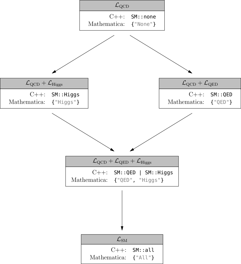
  Figure 2: Possible settings for the beyond_QCD option and the associated Lagrangians defining the perturbative corrections that are included. See eq. (33) for a definition of $\mathcal{L}_{\text{QED}}$ and $\mathcal{L}_{\text{Higgs}}$.

• mass_scheme: Specifies the renormalisation scheme and scale of the quark mass. Note that in the C++ library it is mandatory to specify a scale:

  ⬇

  options opt;

  opt.mass_scheme = {PSshift, 20.};

  opt.mass_scheme = {Pole, 0.};

  For schemes without intrinsic scale (e.g. the pole scheme) the second value can be set arbitrarily. In the Mathematica package, it can also be omitted completely:

  ⬇

  MassScheme -> {"PSshift", 20.}

  MassScheme -> "Pole"

  A list of the available schemes is given in table 3.

  C++ name	Mathematica name	Description
  PS	"PS"	The potential-subtracted insertion scheme
  PSshift	"PSshift"	The potential-subtracted shift scheme
  OneS	"1S"	The 1S insertion scheme
  OneSshift	"1Sshift"	The 1S shift scheme
  Pole	"Pole"	The pole scheme
  MSshift	"MSshift"	The $\overline{\text{MS}}$ scheme

  Table 3: List of available schemes. For details, see section 4.10

• production: Specifies which production channels are taken into account. The possible settings are:

  • photon_only: Production only via a virtual photon. This effectively discards the P-wave contribution from eq. (7), the second term in the vector production operator, and the axialvector production operator defined in eqs. (11) and (12). In addition, box corrections and corrections to the production via a virtual Z boson are discarded in the electroweak contribution to the cross section (eq. (20)).

  • S_wave_only: Production only via an S-wave photon or Z, i.e. the P-wave contribution in eq. (7) is discarded.

  • all: All possible production channels.

  The corresponding Mathematica settings are "PhotonOnly", "SWaveOnly", and "All" (or All).

• expand_s: Specifies the treatment of the overall factor $1/s$ in the polarisation functions defined in eqs. (15), (16) and the electroweak correction (eq. (20)). If set to true, $s=(2\*m_{Q}+E)^{2}$ is expanded in $E/m_{Q}\sim v^{2}\ll 1$ to the appropriate order. This also affects the prefactor $1/s_{N}$ in the residue $Z_{N}$ (eq. (27)).

• double_light_insertion: Specifies whether double insertions (second line of eq. (23)) of the light-quark potential correction $\delta_{C,m_{l}}V$ defined in eq. (25) are taken into account. This option only affects the calculation of the energy levels and residues; in the continuum cross section double insertions are always neglected.

  The impact on observables that can be computed reliably within perturbation theory is typically small. For example, in the determination of the bottom quark mass from the 10th moment of the cross section the end result is changed by about $0.1$ per mille, compared to an overall change of around $0.5$ per mille when combined with the dominant single insertions [38]. In infrared-sensitive quantities like binding energies and residues of bound states with principal quantum number $N>5$ the effects can become significant.

  The calculation of the double insertions is computationally very expensive, requiring the evaluation of an infinite sum over integrals (cf. [38]). Therefore, setting this option to true leads to a considerable slowdown by a factor between $100$ and $1000$. In order to avoid an even more severe slowdown as well as numerical instabilities, the current implementation only computes the first few terms of the sum, so that the result is not very precise. Furthermore, the implementation is not thread safe (cf. section 6.2).

Finally, the default values for version 1.0 of QQbar_threshold are shown in table 4. Since default settings may change in later versions, it is recommended to also consult the online documentation under https://qqbarthreshold.hepforge.org/.

Option	Default for top	Default for bottom
contributions	All set to 1	All set to 1
alpha_s_mZ	alpha_s_mZ = 0.1184	alpha_s_mZ = 0.1184
alpha_s_mu0	(not set)	(not set)
m_Higgs	m_Higgs = 125.	m_Higgs = 125.
Yukawa_factor	1	0
resonant_only	false	true
invariant_mass_cut	$m_{t}-{}$mW	N/A
ml	0	0
r4	824.12 for nl_top = 5	1220.3 for nl_bottom = 4
alpha	alpha_mZ = 1/128.944	alpha_Y = 1/132.274
mu_alpha	mZ = 91.1876	mu_alpha_Y = 10.2
resum_poles	6	6
beyond_QCD	SM::all	SM::QED
mass_scheme	{PSshift, mu_f_top}	{PSshift, mu_f_bottom}
	with mu_f_top = 20.	with mu_f_bottom = 2.
production	production_channel::all	production_channel::all
expand_s	true	false
double_light_insertion	false	false

Table 4: Default option settings in version 1.0 for top and bottom related functions. Variables in the second and third column are defined in the header constants.hpp and can be adjusted during or before installation. The default value for r4 is adjusted automatically if the number of light flavours is changed in constants.hpp.

6 Advanced usage

In the following we discuss several more complicated examples that require some knowledge of the options discussed in section 5 and the structure of the cross section outlined in section 4.

6.1 Wave function at the origin

While the quarkonium wave function at the origin is not a physical observable, it serves as a good example to illustrate some of the more advanced options. Our starting point is eq. (27), the definition of the residue $Z_{N}$. The following assumes that we wish to determine the wave function at the origin in the PS-shift scheme and that the expand_s option is set to false (which is the default for bottom quarks). In a first step, we eliminate $d_{v}$ and the higher-order corrections to $c_{v}$ with the contributions option. We then cancel the remaining prefactor by multiplying with $s_{N}/(4m_{Q}^{2})$, where $m_{Q}$ is the (order-dependent) pole mass computed from $m_{Q}^{\text{PS}}$ according to the shift scheme prescription. To this end, we need to calculate the binding energy $E_{N}^{\text{PS}}$ and convert the input mass from the PS scheme to the pole scheme with the bottom_pole_mass function presented in section 3.5. The following code computes $|\psi_{1}(0)|^{2}=0.721131\,\text{GeV}^{3}$ for the $\Upsilon(1S)$ resonance:

examples/C++/wave_function.cpp

⬇

#include <iostream>

#include "QQbar_threshold/scheme_conversion.hpp"

#include "QQbar_threshold/energy_levels.hpp"

#include "QQbar_threshold/residues.hpp"

int main(){

namespace QQt = QQbar_threshold;

const double mb_PS = 4.5;

const double mu = 4.5;

QQt::options opt = QQt::bottom_options();

opt.contributions.cv = {0., 0., 0.};

opt.contributions.dv = {0., 0.};

const double E_1_PS = QQt::bbbar_energy_level(

1, mu, mb_PS, QQt::N3LO, opt

);

const double s_1 = (2*mb_PS + E_1_PS)*(2*mb_PS + E_1_PS);

const double mb_pole = QQt::bottom_pole_mass(

mu, mb_PS, QQt::N3LO, opt

);

std::cout

<< s_1/(4*mb_pole*mb_pole)*QQt::bbbar_residue(

1, mu, mb_PS, QQt::N3LO, opt

)

<< ’\n’;

}

examples/Mathematica/wave_function.m

⬇

Needs["QQbarThreshold‘"];

With[

{

mbPS = 4.5,

mu = 4.5,

opt = Contributions -> ExceptContributions[

cv -> {0, 0, 0},

dv -> {0, 0}

]

},

E1PS = BBbarEnergyLevel[1, mu, mbPS, "N3LO", opt];

s1 = (2*mbPS + E1PS)^2;

mbPole = BottomPoleMass[mu, mbPS, "N3LO", opt];

Print[s1/(4*mbPole^2)*BBbarResidue[1, mu, mbPS, "N3LO", opt]];

];

Since $s_{N}=(2\*m_{Q}+E_{N})^{2}=(2\*m_{Q}^{\text{PS}}+E_{N}^{\text{PS}})^{2}$ is a scheme-independent quantity we could also have computed the binding energy in the pole scheme and combined it with the pole mass. This method works analogously in the other shift schemes. In an insertion scheme, we proceed the same way. However, in this case one needs to multiply by $s_{N}/(4\*(m_{Q}^{\text{RS}})^{2})$.

6.2 Parallelisation

While the observables for a single given set of parameters can be calculated rather quickly, computing e.g. the cross section over a range of centre-of-mass energies and parameter settings can become somewhat time consuming. In such a situation parallelisation can lead to significant speed-ups.

As an example, we show how to perform a threshold scan similar to the one discussed in section 3.3, but including scale variation. Our strategy is to generate a list containing the centre-of-mass energy, the cross section obtained with a default scale of $80\,$GeV, the minimum and the maximum cross section obtained through scale variation for each point in parallel. Since the mechanisms typically used in C++ vs. Mathematica programs are rather different, we discuss these languages separately in the following sections.

6.2.1 C++

Since we use threads for parallelisation it may be necessary to add additional flags for compilation. The g++ compiler for instance requires the -pthread option:

⬇

g++ -o parallel -std=c++11 parallel.cpp -pthread -lQQbar_threshold

As in the previous examples we use an abbreviation for the somewhat unwieldy QQbar_threshold namespace:

⬇

namespace QQt = QQbar_threshold;

First, we set up a struct comprising the minimum, maximum, and default cross sections obtained for a given centre-of-mass energy:

⬇

struct xs_point{

double sqrt_s;

double xs_default;

double xs_min;

double xs_max;

};

Since we call the cross section function many times with mostly the same arguments, it is also useful to define an auxiliary function that has only the energy and the scale as remaining arguments:

⬇

double xsection(double sqrt_s, double mu){

static constexpr double mu_width = 350.;

static constexpr double mt = 171.5;

static constexpr double width = 1.33;

return QQt::ttbar_xsection(

sqrt_s,

{mu, mu_width},

{mt, width},

QQt::N3LO

);

}

Using this function, we can then define the scale variation for a single centre-of-mass energy. For the sake of simplicity, we use a rather crude sampling of the cross section to estimate the extrema.

⬇

xs_point xsection_scale_variation(double sqrt_s){

static constexpr double mu_default = 80.;

static constexpr double mu_min = 50.;

static constexpr double mu_max = 350.;

static constexpr double mu_step = 5.;

xs_point result;

result.sqrt_s = sqrt_s;

result.xs_default = xsection(sqrt_s, mu_default);

result.xs_min = result.xs_default;

result.xs_max = result.xs_default;

for(double mu = mu_min; mu < mu_max; mu += mu_step){

double current_xsection = xsection(sqrt_s, mu);

if(current_xsection < result.xs_min){

result.xs_min = current_xsection;

}

else if(current_xsection > result.xs_max){

result.xs_max = current_xsection;

}

}

return result;

}

The code to actually calculate the scale variation for various energies in parallel is then rather short:

⬇

std::vector<std::future<xs_point>> results;

for(double sqrt_s = 340.; sqrt_s < 349.; sqrt_s += 0.2){

results.emplace_back(

std::async(

std::launch::async,

xsection_scale_variation, sqrt_s

)

);

}

For each energy, a new thread is launched for computing the scale variation. While this can be rather inefficient in practice, it still ilustrates how parallelisation can be achieved in principle.

To complete the example, we should also include the appropriate headers, load a grid, and produce some output. While all these steps are straightforward, some care should be taken when loading the grid. As already stated in section 3.3, the load_grid function must not be called concurrently from more than one thread. All other functions provided by QQbar_threshold can, however, be safely used in a multithreaded environment. There is one additional exception: if the option double_light_insertion is set to true, the functions for energy levels and residues must not be invoked explicitly from different threads at the same time.

Finally, here is the full code for the parallelised threshold scan with scale variation:

examples/C++/parallel.cpp

⬇

#include <iostream>

#include <iomanip>

#include <vector>

#include <thread>

#include <future>

#include "QQbar_threshold/load_grid.hpp"

#include "QQbar_threshold/xsection.hpp"

namespace QQt = QQbar_threshold;

struct xs_point{

double sqrt_s;

double xs_default;

double xs_min;

double xs_max;

};

double xsection(double sqrt_s, double mu){

static constexpr double mu_width = 350.;

static constexpr double mt = 171.5;

static constexpr double width = 1.33;

return QQt::ttbar_xsection(

sqrt_s,

{mu, mu_width},

{mt, width},

QQt::N3LO

);

}

xs_point xsection_scale_variation(double sqrt_s){

static constexpr double mu_default = 80.;

static constexpr double mu_min = 50.;

static constexpr double mu_max = 350.;

static constexpr double mu_step = 5.;

xs_point result;

result.sqrt_s = sqrt_s;

result.xs_default = xsection(sqrt_s, mu_default);

result.xs_min = result.xs_default;

result.xs_max = result.xs_default;

for(double mu = mu_min; mu < mu_max; mu += mu_step){

double current_xsection = xsection(sqrt_s, mu);

if(current_xsection < result.xs_min){

result.xs_min = current_xsection;

}

else if(current_xsection > result.xs_max){

result.xs_max = current_xsection;

}

}

return result;

}

int main(){

QQt::load_grid(QQt::grid_directory() + "ttbar_grid.tsv");

std::vector<std::future<xs_point>> results;

for(double sqrt_s = 340.; sqrt_s < 349.; sqrt_s += 0.2){

results.emplace_back(

std::async(

std::launch::async,

xsection_scale_variation, sqrt_s

)

);

}

std::cout << std::fixed;

std::cout << "sqrt_s \tcentral \tmin \tmax\n";

for(auto & res: results){

xs_point current_point = res.get();

std::cout << current_point.sqrt_s << ’\t’

<< current_point.xs_default << ’\t’

<< current_point.xs_min << ’\t’

<< current_point.xs_max << ’\n’;

}

}

6.2.2 Mathematica

For parallelisation in Mathematica, we have to ensure that each kernel knows all relevant definitions and has its own precomputed grid:

⬇

Needs["QQbarThreshold‘"];

LaunchKernels[];

ParallelEvaluate[Needs["QQbarThreshold‘"]];

ParallelEvaluate[LoadGrid[GridDirectory <> "ttbar_grid.tsv"]];

This is very different from the parallelisation at thread level we used in the C++ case. In the present example, the kernels are independent processes and therefore unable to share a common grid. It is not only safe, but even necessary to load multiple copies of a grid at the same time.

For the actual threshold scan, we first define an auxiliary function for the cross section with fixed top quark properties and width scale:

⬇

XSection[sqrts_, mu_] := With[

{muWidth = 350, mt = 171.5, width = 1.33},

TTbarXSection[sqrts, {mu, muWidth}, {mt, width}, "N3LO"]

];

To perform the scale variation, we use Mathematica’s built-in NMinValue and NMaxValue functions:

⬇

XSectionScaleVariation[sqrts_] := Module[

{

muDefault = 80, muMin = 50, muMax = 350,

xsDefault, xsMin, xsMax, mu

},

xsDefault = XSection[sqrts, muDefault];

xsMin = NMinValue[

{XSection[sqrts, mu], muMin <= mu <= muMax},

mu,

Method -> "SimulatedAnnealing"

];

xsMax = NMaxValue[

{XSection[sqrts, mu], muMin <= mu <= muMax},

mu,

Method -> "SimulatedAnnealing"

];

Return[{sqrts, xsDefault, xsMin, xsMax}];

];

After this, the code for the actual parallelised scan is again rather compact:

⬇

results = ParallelTable[

XSectionScaleVariation[sqrts],

{sqrts, 340, 349, 0.2}

];

We complete the example by adding some code for the output:

examples/Mathematica/parallel.m

⬇

LaunchKernels[];

Needs["QQbarThreshold‘"];

ParallelEvaluate[Needs["QQbarThreshold‘"]];

ParallelEvaluate[LoadGrid[GridDirectory <> "ttbar_grid.tsv"]];

XSection[sqrts_, mu_] := With[

{muWidth = 350, mt = 171.5, width = 1.33},

TTbarXSection[sqrts, {mu, muWidth}, {mt, width}, "N3LO"]

];

XSectionScaleVariation[sqrts_] := Module[

{

muDefault = 80, muMin = 50, muMax = 350,

xsDefault, xsMin, xsMax, mu

},

xsDefault = XSection[sqrts, muDefault];

xsMin = NMinValue[

{XSection[sqrts, mu], muMin <= mu <= muMax},

mu,

Method -> "SimulatedAnnealing"

];

xsMax = NMaxValue[

{XSection[sqrts, mu], muMin <= mu <= muMax},

mu,

Method -> "SimulatedAnnealing"

];

Return[{sqrts, xsDefault, xsMin, xsMax}];

];

results = ParallelTable[

XSectionScaleVariation[sqrts],

{sqrts, 340, 349, 0.2}

];

PrependTo[results, {"sqrt_s", "central", "min", "max"}];

Print[TableForm[results]];

6.3 Moments for nonrelativistic sum rules

Next to threshold scans for $t\bar{t}$ production, the calculation of moments for $\Upsilon$ sum rules is one of the key applications for QQbar_threshold. It is conventional to consider the normalised cross section (cf. eq. (5)) $R_{b}=\sigma_{b}/\sigma_{pt}$ with $\sigma_{pt}=4\*\pi\*\alpha(\mu_{\alpha})^{2}/(3\*s)$, which can be calculated with the bbbar_R_ratio function. The moments of $R_{b}$ are then defined as

$${\cal M}_{n}=\int_{0}^{\infty}\frac{R_{b}(s)}{s^{n+1}}\,.$$ (35)

Splitting the moments into the contribution from the narrow $\Upsilon$ resonances and the remaining continuum contribution we obtain

$${\cal M}_{n}=\frac{12\pi^{2}N_{c}e_{b}^{2}}{m_{b}^{2}}\sum_{N=1}^{\infty}\frac{Z_{N}}{s_{N}^{2\*n+1}}+\int_{4\*m_{b}^{2}}^{\infty}ds\,\frac{R_{b}(s)}{s^{n+1}}\,.$$ (36)

We now show how this formula can be evaluated with QQbar_threshold. Since discussing numerical integration is clearly outside the scope of this work, we assume the existence of a C++ header integral.hpp that provides a suitable integral function. The example code moments.cpp distributed together with QQbar_threshold in fact includes such a header. Since this header uses the GSL library, the code example has to be compiled with additional linker flags, e.g.

⬇

g++ -o moments -std=c++11 moments.cpp -lQQbar_threshold -lgsl -lgslcblas

For the sake of simplicity, we use the standard bottom options and only keep the bottom quark mass and $n$ as free parameters in our example. We can then define auxiliary functions for the energy levels, residues, and the continuum cross section:

⬇

static constexpr double pi = 3.14159265358979323846264338328;

double Z(int N, double mb_PS){

return QQt::bbbar_residue(N, mb_PS, mb_PS, QQt::N3LO);

}

double E(int N, double mb_PS){

return QQt::bbbar_energy_level(N, mb_PS, mb_PS, QQt::N3LO);

}

double Rb(double s, double mb_PS){

try{

return QQt::bbbar_R_ratio(std::sqrt(s), mb_PS, mb_PS, QQt::N3LO);

}

catch(std::out_of_range){

return std::numeric_limits<double>::quiet_NaN();

}

}

Note that for the bottom cross section we have to handle the case that the centre-of-mass energy is outside the region covered by the precomputed grid. In fact, we assume that the value obtained for the continuum integral in eq. (36) is reliable in spite of the limited grid size. For a more careful analysis, this assumption should of course be checked, for example by varying the upper bound of the integral.

Let us first consider the resonance contribution. For the prefactor, we have to convert the input mass from the PS scheme to the pole scheme, which can be done with the function bottom_pole_mass (see section 3.5). The remaining code is then rather straightforward:

⬇

double M_resonances(int n, double mb_PS){

static constexpr int N_c = 3;

static constexpr double e_b = QQt::e_d;

double sum_N = 0.0;

for(int N = 1; N <= 6; ++ N){

sum_N += Z(N, mb_PS)*std::pow(2*mb_PS + E(N, mb_PS), -2*n-1);

}

const double mb_pole = QQt::bottom_pole_mass(mb_PS, mb_PS, QQt::N3LO);

return 12*pi*pi*N_c*e_b*e_b/(mb_pole*mb_pole)*sum_N;

}

Since at N³LO, only the first six resonances can be computed with QQbar_threshold, we have cut off the sum at $N=6$.

For the continuum contribution, we encounter the problem that typical C++ integration routines can only evaluate integrals over a finite interval. To deal with this we perform a substitution, e.g. $s=s(x)=4\*m_{b}^{2}+\frac{x}{1-x}$, so we have

$$\int_{4\*m_{b}^{2}}^{\infty}ds\,\frac{R_{b}(s)}{s^{n+1}}=\int_{0}^{1}\frac{dx}{(1-x)^{2}}\frac{R_{b}\big{(}s(x)\big{)}}{s(x)^{n+1}}\,.$$ (37)

The continuum moments can then be computed with the following code:

⬇

double M_continuum(int n, double mb_PS){

double const s0 =

pow(QQt::bbbar_threshold(mb_PS, mb_PS, QQt::N3LO), 2);

auto s = [=](double x){

return s0 + x/(1-x);

};

auto integrand = [=](double x){

return Rb(s(x), mb_PS)*std::pow(s(x), -n-1)*std::pow(1 - x, -2);

};

return integral(0, 1, integrand);

}

All that remains is then to add up both contributions and add the standard boilerplate code for including headers, loading the grid, etc. It is also convenient to rescale the moments to be of order one. For this, we multiply them by a factor of $(10\,\text{GeV})^{2\*n}$. Finally, here is the complete code for our example:

examples/C++/moments.cpp

⬇

#include <cmath>

#include <limits>

#include <iostream>

#include "QQbar_threshold/load_grid.hpp"

#include "QQbar_threshold/xsection.hpp"

#include "QQbar_threshold/threshold.hpp"

#include "QQbar_threshold/residues.hpp"

#include "QQbar_threshold/energy_levels.hpp"

#include "QQbar_threshold/scheme_conversion.hpp"

#include "integral.hpp"

namespace QQt = QQbar_threshold;

static constexpr double pi = 3.14159265358979323846264338328;

double Z(int N, double mb_PS){

return QQt::bbbar_residue(N, mb_PS, mb_PS, QQt::N3LO);

}

double E(int N, double mb_PS){

return QQt::bbbar_energy_level(N, mb_PS, mb_PS, QQt::N3LO);

}

double Rb(double s, double mb_PS){

try{

return QQt::bbbar_R_ratio(std::sqrt(s), mb_PS, mb_PS, QQt::N3LO);

}

catch(std::out_of_range){

return std::numeric_limits<double>::quiet_NaN();

}

}

double M_resonances(int n, double mb_PS){

static constexpr int N_c = 3;

static constexpr double e_b = QQt::e_d;

double sum_N = 0.0;

for(int N = 1; N <= 6; ++ N){

sum_N += Z(N, mb_PS)*std::pow(2*mb_PS + E(N, mb_PS), -2*n-1);

}

const double mb_pole = QQt::bottom_pole_mass(mb_PS, mb_PS, QQt::N3LO);

return 12*pi*pi*N_c*e_b*e_b/(mb_pole*mb_pole)*sum_N;

}

double M_continuum(int n, double mb_PS){

double const s0 =

pow(QQt::bbbar_threshold(mb_PS, mb_PS, QQt::N3LO), 2);

auto s = [=](double x){

return s0 + x/(1-x);

};

auto integrand = [=](double x){

return Rb(s(x), mb_PS)*std::pow(s(x), -n-1)*std::pow(1 - x, -2);

};

return integral(0, 1, integrand);

}

double M(int n, double mb_PS){

return pow(10, 2*n)*(M_resonances(n, mb_PS) + M_continuum(n, mb_PS));

}

int main(){

QQt::load_grid(QQt::grid_directory() + "bbbar_grid_large.tsv");

std::cout << M(10, 4.5322) << ’\n’;

}

In units of $(10\,\text{GeV})^{-20}$, we find ${\cal M}_{10}=0.264758$, which is in good agreement with the experimental value ${\cal M}_{10}=0.2648(36)$. In other words, our determination of the PS mass agrees very well with the central value $m_{b}^{\text{PS}}=4.532\,$GeV found in [38].

For Mathematica, the structure is quite similar. To avoid clashes with built-in functions, we have renamed some of the variables.

examples/Mathematica/moments.m

⬇

Needs["QQbarThreshold‘"];

ZN[i_, mbPS_] := BBbarResidue[i, mbPS, mbPS, "N3LO"];

EN[i_, mbPS_] := BBbarEnergyLevel[i, mbPS, mbPS, "N3LO"];

Rb[s_, mbPS_] := BBbarRRatio[Sqrt[s], mbPS, mbPS, "N3LO"];

Mresonances[n_, mbPS_] := With[

{

Nc = 3, eb = eD,

mbPole = BottomPoleMass[mbPS, mbPS, "N3LO"]

},

12*Pi^2*Nc*eb^2/mbPole^2*Sum[

ZN[i, mbPS]/(2*mbPS + EN[i, mbPS])^(2*n+1),

{i, 1, 6}

]

];

Mcontinuum[n_, mbPS_] := Module[

{s0, s, x},

s0 = BBbarThreshold[mbPS, mbPS, "N3LO"]^2;

s[x_] := s0 + x/(1 - x);

Return[

NIntegrate[

Rb[s[x], mbPS]/(s[x]^(n+1)*(1 - x)^2),

{x, 0, 1},

AccuracyGoal -> 5

]

];

];

M[n_, mbPS_] := 10^(2*n)*(Mresonances[n, mbPS] + Mcontinuum[n, mbPS]);

LoadGrid[GridDirectory <> "bbbar_grid_large.tsv"];

Print[M[10, 4.5322]];

Here, we obtain a slightly different value of ${\cal M}_{10}=0.264857$, which stems from a different integration algorithm. Since this change can be offset by changing the input mass by a small amount of about $0.1\,$MeV, we can conclude that integration errors are under control.

7 Grid generation

Depending on the chosen input parameters, the precomputed grids distributed with QQbar_threshold may not be sufficient. In these cases custom grids can be generated with the QQbarGridCalc package, which can be downloaded separately from https://www.hepforge.org/downloads/qqbarthreshold/ and needs no special installation aside from unpacking the archive with tar xzf QQbarGridCalc.tar.gz. Grid generation requires Wolfram Mathematica. The Mathematica working directory should be set to the QQbarGridCalc directory (e.g. with the SetDirectory command), so that all included files are found.

7.1 Top and bottom grids

The main function provided by this package is QQbarCalcGrid, which generates a grid for the bottom or top cross section. It can be used in the following way:

⬇

QQbarCalcGrid[

Energy -> {MinEnergy, MaxEnergy, EnergyStep},

Width -> {MinWidth, MaxWidth, WidthStep},

"GridFileName"

];

MinEnergy and MaxEnergy refer to the naïve threshold at $\sqrt{s}=2m_{Q}$, where $m_{Q}$ is the heavy-quark pole mass. The generated grid thus covers the centre-of-mass energies $2m_{Q}+\mathtt{MinEnergy}\leq\sqrt{s}\leq 2m_{Q}+\mathtt{MaxEnergy}$ and the widths $\mathtt{MinWidth}\leq\Gamma\leq\mathtt{MaxWidth}$. EnergyStep and WidthStep specify the distance between adjacent grid points. The resulting grid is saved in the file GridFileName. For example, the following program creates a small top grid and exports it to the file top_grid_example.tsv:

examples/Mathematica/top_grid_simple.m

⬇

<<QQbarGridCalc.m;

LaunchKernels[];

QQbarCalcGrid[

Energy -> {-1, 1, 1},

Width -> {1.5, 1.6, 0.1},

"top_grid_example.tsv"

];

Note that loading the package typically takes several minutes. The calculation of the grids themselves is even more time-consuming, so we restrict the examples to very small and coarse grids and suggest to rely on parallelisation as much as possible.

The energy and width ranges always refer to reference values for the quark mass and the strong coupling, specified with the QuarkMass and AlphaS options (defaulting to 175 and 0.14, respectively). In fact, internally all energies and widths are rescaled by a factor of $-m_{Q}\*\alpha_{s}^{2}\*C_{F}^{2}/4$. In practice, this implies that the range covered in the actual calculation of the cross section will in general be slightly different. Furthermore, the default values for QuarkMass and AlphaS are chosen with top grids in mind, so one should change these settings when calculating bottom grids.

In some cases it is desirable to have grids that are relatively coarse in one region, e.g. at high energies, and much finer in another region. To this end it is possible to directly specify the energy and width points when calling QQbarCalcGrid as

⬇

QQbarCalcGrid[

Energy -> {{EnergiesPts … }},

Width -> {{WidthPts … }},

"GridFileName"

];

The following example shows how a bottom grid with a higher resolution close to the threshold can be generated:

examples/Mathematica/bottom_grid.m

⬇

<<QQbarGridCalc.m;

LaunchKernels[];

emin = 10^-6;

emax = 10;

n = 3;

epoints = Module[

{stepfact},

stepfact = (emax/emin)^(1/(n - 1));

Table[N[emin*stepfact^i], {i, 0, n - 1}]

];

QQbarCalcGrid[

Energy -> {epoints},

Width -> {{10^-10, 10^-8}},

"bottom_grid_example.tsv",

QuarkMass -> 5,

AlphaS -> 0.25

];

Note that the numerical evaluation requires at least a small non-vanishing width, which is internally set to $10^{-9}$ for bottom quarks. For such a small width it is not possible (and not very useful) to calculate grid points with negative energies.

Finally, QQbarCalcGrid offers the Comments option to prepend custom comments to the generated grid file:

⬇

QQbarCalcGrid[

Energy -> {…},

Width -> {…},

"GridFileName",

Comments -> {

"Comment in the first line of the grid file",

"Comment in the second line of the grid file"

}

];

The default setting Comment -> Automatic adds the version of QQbarCalcGrid, a shortened version of the command used for the creation, and the creation date.

7.2 Nonresonant grids

The second function in QQbarGridCalc, QQbarCalcNonresonantGrid, allows the generation of grids for the nonresonant cross section (see section 4.3). Its syntax is similar to QQbarCalcGrid:

⬇

QQbarCalcNonresonantGrid[

MassRatio -> {…},

Cut -> {…},

"GridFileName"

];

As with QQbarCalcGrid both regular and irregular grids can be generated and also the Comment option is supported. The first argument specifies the mass ratios $x=m_{W}/m_{Q}$, whereas the second argument determines the invariant mass cut. The coordinates entered here correspond to $y_{w}=(1-y)/(1-x)$, where $y=(1-\Delta_{m}/m_{Q})^{2}$ and $\Delta_{m}$ is the cut specified by the invariant_mass_cut option (see section 5). Thus, for physical cuts $0\leq y_{w}\leq 1$. The default built-in nonresonant grid can be reproduced with the following program:

examples/Mathematica/nonresonant_grid.m

⬇

<<QQbarGridCalc.m;

LaunchKernels[];

QQbarCalcNonresonantGrid[

MassRatio -> {0.15, 0.30, 0.01},

Cut -> {0, 1, 0.01},

"non-resonant_grid.tsv"

];

Appendix A Predefined constants

Table 5 lists all predefined constants and their values. The values can be adjusted prior to or during the installation of the QQbar_threshold library.

C++ name	Mathematica name	Value	Description
$\dagger$ alpha_s_mZ	alphaSmZDefault	$0.1184$	Default value for strong coupling at the scale mZ.
$\dagger$ alpha_mZ	alphamZ	$1/128.944$	QED coupling at the scale mZ.
$\dagger$ alpha_Y	alphaY	$1/132.274$	QED coupling at the scale mu_alpha_Y.
$\dagger$ mu_alpha_Y	muAlphaY	$10.2$	Typical scale for $\Upsilon$ resonances.
mZ	mZ	$91.1876$	Mass of the Z boson.
mW	mW	$80.385$	Mass of the W boson.
G_F	GF	$1.1663787\times 10^{-5}$	Fermi constant. Only used for calculating the top width.
$\dagger$ m_Higgs	mHiggsDefault	$125$	Default value for mass of the Higgs boson.
alpha_QED	alphaQED	$1/137.035999074$	Fine structure constant.
e_u	eU	$2/3$	Electric charge of the top quark in units of the positron charge.
e_d	eD	$-1/3$	Electric charge of the bottom quark.
e	eE	$-1$	Electric charge of the electron.
cw2	cw2	mW^2/mZ^2	Cosine of the weak mixing angle squared.
sw2	sw2	1 - cw2	Sine of the weak mixing angle squared.
T3_nu	T3Nu	$1/2$	Weak isospin of neutrino.
T3_e	T3E	$-1/2$	Weak isospin of electron.
T3_u	T3U	$1/2$	Weak isospin of top.
T3_d	T3D	$-1/2$	Weak isospin of bottom.
mb_SI	mbSI	$4.203$	Reference scale-invariant mass for bottom quarks.
mu_thr	muThr	2*mb_SI	Decoupling threshold for bottom quarks.
nl_bottom	nlBottom	$4$	Number of light flavours for bottom-related functions.
nl_top	nlTop	$5$	Number of light flavours for top-related functions.
$\dagger$ mu_f_bottom	mufBottom	$2$	Default PS scale for bottom.
$\dagger$ mu_f_top	mufTop	$20$	Default PS scale for top.
invGeV2_to_pb	InvGeV2ToPb	$389379300$	Conversion factor from GeV-2 to picobarn.

Table 5: Constants predefined in the constants.hpp header. Entries marked with a $\dagger$ only serve as default values and can be overridden through option settings (cf. section 5).

References

- [1] K. Seidel, F. Simon, M. Tesar, S. Poss, Top quark mass measurements at and above threshold at CLIC, Eur. Phys. J. C73 (8) (2013) 2530. arXiv:1303.3758.
- [2] F. Simon, A First Look at the Impact of NNNLO Theory Uncertainties on Top Mass Measurements at the ILC, in: International Workshop on Future Linear Colliders (LCWS15) Whistler, B.C., Canada, November 2-6, 2015, 2016. arXiv:1603.04764.
- [3] V. Novikov, L. Okun, M. A. Shifman, A. Vainshtein, M. Voloshin, V. I. Zakharov, Sum rules for charmonium and charmed mesons decay rates in quantum chromodynamics, Phys. Rev. Lett. 38 (1977) 626.
- [4] V. Novikov, L. Okun, M. A. Shifman, A. Vainshtein, M. Voloshin, V. I. Zakharov, Charmonium and gluons: Basic experimental facts and theoretical introduction, Phys. Rept. 41 (1978) 1–133.
- [5] M. B. Voloshin, Yu. M. Zaitsev, Physics of resonances: Ten years later, Sov. Phys. Usp. 30 (1987) 553–574, [Usp. Fiz. Nauk 152 (1987) 361].
- [6] A. Pineda, J. Soto, Effective field theory for ultrasoft momenta in NRQCD and NRQED, Nucl. Phys. Proc. Suppl. 64 (1998) 428–432. arXiv:hep-ph/9707481.
- [7] M. E. Luke, A. V. Manohar, I. Z. Rothstein, Renormalization group scaling in nonrelativistic QCD, Phys. Rev. D61 (2000) 074025. arXiv:hep-ph/9910209.
- [8] A. H. Hoang, et al., Top - anti-top pair production close to threshold: Synopsis of recent NNLO results, Eur. Phys. J.direct C3 (2000) 1–22. arXiv:hep-ph/0001286.
- [9] M. Beneke, Y. Kiyo, P. Marquard, A. Penin, J. Piclum, M. Steinhauser, Next-to-Next-to-Next-to-Leading Order QCD Prediction for the Top Antitop -Wave Pair Production Cross Section Near Threshold in Annihilation, Phys. Rev. Lett. 115 (19) (2015) 192001. arXiv:1506.06864.
- [10] M. Beneke, J. Piclum, T. Rauh, P-wave contribution to third-order top-quark pair production near threshold, Nucl. Phys. B880 (2014) 414–434. arXiv:1312.4792.
- [11] M. Beneke, B. Jantzen, P. Ruiz-Femenía, Electroweak non-resonant NLO corrections to in the resonance region, Nucl. Phys. B840 (2010) 186–213. arXiv:1004.2188.
- [12] A. A. Penin, J. H. Piclum, Threshold production of unstable top, JHEP 01 (2012) 034. arXiv:1110.1970.
- [13] B. Jantzen, P. Ruiz-Femenía, Next-to-next-to-leading order nonresonant corrections to threshold top-pair production from collisions: Endpoint-singular terms, Phys.Rev. D88 (5) (2013) 054011. arXiv:1307.4337.
- [14] P. Ruiz-Femenía, First estimate of the NNLO nonresonant corrections to top-antitop threshold production at lepton colliders, Phys. Rev. D89 (9) (2014) 097501. arXiv:1402.1123.
- [15] M. J. Strassler, M. E. Peskin, The Heavy top quark threshold: QCD and the Higgs, Phys. Rev. D43 (1991) 1500–1514.
- [16] R. J. Guth, J. H. Kühn, Top quark threshold and radiative corrections, Nucl. Phys. B368 (1992) 38–56.
- [17] R. Harlander, M. Jeżabek, J. H. Kühn, Higgs effects in top quark pair production, Acta Phys. Polon. B27 (1996) 1781–1788. arXiv:hep-ph/9506292.
- [18] D. Eiras, M. Steinhauser, Complete Higgs mass dependence of top quark pair threshold production to order , Nucl. Phys. B757 (2006) 197–210. arXiv:hep-ph/0605227.
- [19] M. Beneke, A. Maier, J. Piclum, T. Rauh, Higgs effects in top anti-top production near threshold in annihilation, Nucl. Phys. B899 (2015) 180–193. arXiv:1506.06865.
- [20] B. Grza̧dkowski, J. H. Kühn, P. Krawczyk, R. G. Stuart, Electroweak Corrections on the Toponium Resonance, Nucl. Phys. B281 (1987) 18.
- [21] A. H. Hoang, C. J. Reißer, Electroweak absorptive parts in NRQCD matching conditions, Phys. Rev. D71 (2005) 074022. arXiv:hep-ph/0412258.
- [22] A. H. Hoang, C. J. Reißer, On electroweak matching conditions for top pair production at threshold, Phys. Rev. D74 (2006) 034002. arXiv:hep-ph/0604104.
- [23] A. Denner, T. Sack, The Top width, Nucl. Phys. B358 (1991) 46–58.
- [24] G. Eilam, R. R. Mendel, R. Migneron, A. Soni, Radiative corrections to top quark decay, Phys. Rev. Lett. 66 (1991) 3105–3108.
- [25] M. Jeżabek, J. H. Kühn, The Top width: Theoretical update, Phys. Rev. D48 (1993) 1910–1913, [Erratum: Phys. Rev. D49 (1994) 4970]. arXiv:hep-ph/9302295.
- [26] M. Fischer, S. Groote, J. G. Körner, M. C. Mauser, Longitudinal, transverse plus and transverse minus bosons in unpolarized top quark decays at , Phys. Rev. D63 (2001) 031501. arXiv:hep-ph/0011075.
- [27] I. R. Blokland, A. Czarnecki, M. Slusarczyk, F. Tkachov, Next-to-next-to-leading order calculations for heavy-to-light decays, Phys. Rev. D71 (2005) 054004, [Erratum: Phys. Rev. D79 (2009) 019901]. arXiv:hep-ph/0503039.
- [28] M. Beneke, Y. Kiyo, K. Schuller, Third-order correction to top-quark pair production near threshold I. Effective theory set-up and matching coefficients. arXiv:1312.4791.
- [29] M. Beneke, Y. Kiyo, K. Schuller, Third-order correction to top-quark pair production near threshold II. Potential contributions, In preparation.
- [30] M. Beneke, A. P. Chapovsky, A. Signer, G. Zanderighi, Effective theory approach to unstable particle production, Phys. Rev. Lett. 93 (2004) 011602. arXiv:hep-ph/0312331.
- [31] M. Beneke, A. P. Chapovsky, A. Signer, G. Zanderighi, Effective theory calculation of resonant high-energy scattering, Nucl. Phys. B686 (2004) 205–247. arXiv:hep-ph/0401002.
- [32] M. Beneke, A. Signer, V. A. Smirnov, Top quark production near threshold and the top quark mass, Phys. Lett. B454 (1999) 137–146. arXiv:hep-ph/9903260.
- [33] P. Marquard, J. H. Piclum, D. Seidel, M. Steinhauser, Three-loop matching of the vector current, Phys. Rev. D89 (3) (2014) 034027. arXiv:1401.3004.
- [34] M. Beneke, Y. Kiyo, K. Schuller, Third-order Coulomb corrections to the S-wave Green function, energy levels and wave functions at the origin, Nucl. Phys. B714 (2005) 67–90. arXiv:hep-ph/0501289.
- [35] M. Melles, Massive fermionic corrections to the heavy quark potential through two loops, Phys. Rev. D58 (1998) 114004. arXiv:hep-ph/9805216.
- [36] M. Melles, The static QCD potential in coordinate space with quark masses through two loops, Phys. Rev. D62 (2000) 074019. arXiv:hep-ph/0001295.
- [37] A. Hoang, Bottom quark mass from mesons: Charm mass effects, arXiv:hep-ph/0008102.
- [38] M. Beneke, A. Maier, J. Piclum, T. Rauh, The bottom-quark mass from non-relativistic sum rules at NNNLO, Nucl. Phys. B891 (2015) 42–72. arXiv:1411.3132.
- [39] M. Beneke, A quark mass definition adequate for threshold problems, Phys. Lett. B434 (1998) 115–125. arXiv:hep-ph/9804241.
- [40] A. H. Hoang, Z. Ligeti, A. V. Manohar, decay and the mass, Phys. Rev. Lett. 82 (1999) 277–280. arXiv:hep-ph/9809423.
- [41] P. Marquard, A. V. Smirnov, V. A. Smirnov, M. Steinhauser, Quark Mass Relations to Four-Loop Order in Perturbative QCD, Phys. Rev. Lett. 114 (14) (2015) 142002. arXiv:1502.01030.
- [42] S. Bekavac, A. Grozin, D. Seidel, M. Steinhauser, Light quark mass effects in the on-shell renormalization constants, JHEP 0710 (2007) 006. arXiv:0708.1729.