Joint transverse momentum and threshold resummation beyond NLL

Abstract

To describe the transverse momentum spectrum of heavy color-singlet production, the joint resummation of threshold and transverse momentum logarithms is investigated. We obtain factorization theorems for various kinematic regimes valid to all orders in the strong coupling, using Soft-Collinear Effective Theory. We discuss how these enable resummation and how to combine regimes. The new ingredients in the factorization theorems are calculated at next-to-leading order, and a range of consistency checks is performed. Our framework goes beyond the current next-to-leading logarithmic accuracy (NLL).

I Introduction

In heavy particle production the additional radiation tends to be soft, due to the steeply falling parton distribution functions (PDFs). This implies that threshold logarithms of $1-z\equiv 1-Q^{2}/\hat{s}$ in the partonic cross section are large, where $Q$ is the heavy particle invariant mass and $\hat{s}$ the partonic center-of-mass energy. The corresponding threshold resummation can significantly modify the cross section. Well-known examples are top-quark pair production or the production of supersymmetric particles. When the $p_{T}$ of the heavy particle(s) is parametrically smaller than $Q$, the transverse momentum resummation of the logarithms of $p_{T}/Q$ is important as well.

In this letter we study the joint resummation of threshold and transverse momentum logarithms. A formalism that achieves this at next-to-leading logarithmic (NLL) order has been developed some time ago Laenen et al. (2001) (see also Ref. Li (1999)). Here resummation is simultaneously performed in Mellin moment (of $z$) and impact parameter (Fourier conjugate to $p_{T}$), accounting for the recoil of soft gluons using non-Abelian exponentiation and including the recoil in the kinematics of the hard scattering. This framework has been applied to prompt-photon Laenen et al. (2000), electroweak Kulesza et al. (2002), Higgs boson Kulesza et al. (2004), heavy-quark Banfi and Laenen (2005), slepton pair Bozzi et al. (2008) and gaugino pair Debove et al. (2011) production.

We introduce a framework for joint resummation using Soft-Collinear Effective Theory (SCET) Bauer et al. (2000, 2001); Bauer and Stewart (2001); Bauer et al. (2002a, b); Beneke et al. (2002), which enables us to go beyond NLL. We need to assume a relative power counting between the threshold parameter $1\!-\!z$ and transverse momentum $p_{T}\gg\Lambda_{\mathrm{QCD}}$ to derive factorization theorems, and identify the following three regimes

1. $1\sim 1-z\gg p_{T}/Q$: transverse mom. factorization

2. $1\gg 1-z\gg p_{T}/Q$: ​intermediate regime

3. $1\gg 1-z\sim p_{T}/Q$: threshold factorization

The factorization theorems for regimes 1 and 3 are simply a more differential version of the standard transverse momentum and threshold resummation. The intermediate regime 2 requires us to extend SCET with additional collinear-soft (csoft) degrees of freedom. Such theories, typically referred to as ${\rm SCET}_{+}$, have recently been used to describe a range of joint resummations Bauer et al. (2012); Procura et al. (2015); Larkoski et al. (2015a, b); Becher et al. (2015); Chien et al. (2016); Pietrulewicz et al. (2016). We will elaborate on how the factorization in SCET leads to resummation using the renormalization group (RG) evolution. As a byproduct, this implies an all-order relation between the anomalous dimension of the thrust soft function and threshold soft function. We discuss how to combine the different factorization theorems describing the three regimes, finding that regime 2 can be obtained from regime 1 by a proper modification of renormalization scales, but that regime 3 contains additional corrections beyond NLL. By using SCET, gauge invariance is manifest, and the ingredients in factorization theorems have matrix element definitions. We will focus on the production of a color neutral state $pp\to V+X$ with $V=Z,W,h,\dots$, working in momentum space. All ingredients will be collected for joint resummation at next-to-next-to-leading logarithmic order (NNLL).

This letter is organized as follows. In Sec. II we present the factorization theorem for joint resummation in each regime, and derive consistency relations between them. All ingredients entering the factorization formula are collected at next-to-leading order (NLO) in Sec. III, and the consistency between regimes is verified. The renormalization group equations are given in Sec. IV, providing an internal consistency check on each individual regime. In Sec. V we discuss how to perform the resummation and combine the cross section in the three regimes. We conclude in Sec. VI.

II Factorization

In this section we present the factorization theorems that enable the joint resummation of threshold and transverse momentum logarithms, address a subtlety that arises at partonic threshold, and derive consistency relations between the regimes.

II.1 Factorization theorems

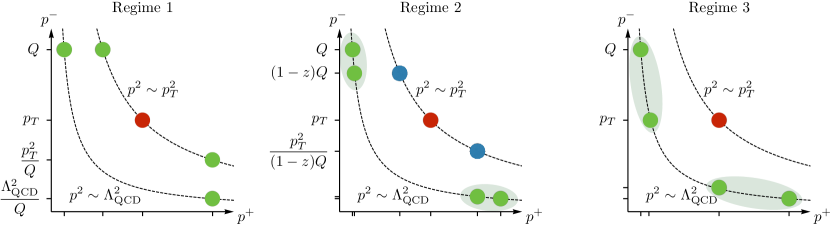
Figure 1: The power counting of collinear (green), collinear-soft (blue) and soft (red) modes for the three regimes. The dashed lines show invariant mass hyperbolas, and the nonperturbative modes that we do not factorize are grouped together.

Regime:	1: $Q\sim(1-z)Q\gg p_{T}\gg\Lambda_{\mathrm{QCD}}$	2: $Q\gg(1-z)Q\gg p_{T}\gg\Lambda_{\mathrm{QCD}}$	3: $Q\sim(1-z)Q\sim p_{T}\gg\Lambda_{\mathrm{QCD}}$
$n$-collinear	$(\Lambda_{\mathrm{QCD}}^{2}/Q,Q,\Lambda_{\mathrm{QCD}})$	$(\Lambda_{\mathrm{QCD}}^{2}/Q,Q,\Lambda_{\mathrm{QCD}})$	$(\Lambda_{\mathrm{QCD}}^{2}/Q,Q,\Lambda_{\mathrm{QCD}})$
	$(p_{T}^{2}/Q,Q,p_{T})$	$\bigl{(}\Lambda_{\mathrm{QCD}}^{2}/[(1-z)Q],(1-z)Q,\Lambda_{\mathrm{QCD}}\bigr{)}$	$\bigl{(}\Lambda_{\mathrm{QCD}}^{2}/[(1-z)Q],(1-z)Q,\Lambda_{\mathrm{QCD}}\bigr{)}$
${\bar{n}}$-collinear	$(Q,\Lambda_{\mathrm{QCD}}^{2}/Q,\Lambda_{\mathrm{QCD}})$	$(Q,\Lambda_{\mathrm{QCD}}^{2}/Q,\Lambda_{\mathrm{QCD}})$	$(Q,\Lambda_{\mathrm{QCD}}^{2}/Q,\Lambda_{\mathrm{QCD}})$
	$(Q,p_{T}^{2}/Q,p_{T})$	$\quad\bigl{(}(1-z)Q,\Lambda_{\mathrm{QCD}}^{2}/[(1-z)Q],\Lambda_{\mathrm{QCD}}\bigr{)}\quad$	$\bigl{(}(1-z)Q,\Lambda_{\mathrm{QCD}}^{2}/[(1-z)Q],\Lambda_{\mathrm{QCD}}\bigr{)}$
$n$-csoft		$\bigl{(}p_{T}^{2}/[(1-z)Q],(1-z)Q,p_{T}\bigr{)}$
${\bar{n}}$-csoft		$\bigl{(}(1-z)Q,p_{T}^{2}/[(1-z)Q],p_{T}\bigr{)}$
soft	$(p_{T},p_{T},p_{T})$	$(p_{T},p_{T},p_{T})$	$(p_{T},p_{T},p_{T})$

Table 1: The modes (rows) and power counting of momenta in light-cone coordinates Eq. (1), for the three regimes (columns).

In the introduction we identified three kinematic regimes, depending on the relative power counting of the transverse momentum and threshold parameter. The corresponding modes are shown in Fig. 1 and are summarized in Table 1, using light-cone coordinates

$$p^{\mu}=(p^{+},p^{-},p_{\perp}^{\mu})=(p^{0}-p^{3},p^{0}+p^{3},p_{\perp}^{\mu})\,.$$ (1)

We illustrate the origin of these degrees of freedom for regime 2. The incoming proton in the $n^{\mu}=(1,0,0,1)$ direction is described by a mode whose momentum components have the parametric size $(p^{+},p^{-},p_{\perp}^{\mu})\sim(\Lambda_{\mathrm{QCD}}^{2}/Q,Q,\Lambda_{\mathrm{QCD}})$. This scaling is fixed by its energy $\sim Q$ and virtuality $\sim\Lambda_{\mathrm{QCD}}$. Since we are in the threshold limit, the energy of the real radiation is $\lesssim(1-z)Q$. Collinear splittings within the proton therefore require an additional mode $(\Lambda_{\mathrm{QCD}}^{2}/[(1-z)Q],(1-z)Q,\Lambda_{\mathrm{QCD}})$. It is natural to combine these nonperturbative modes into the (threshold) PDF, as they are both required for the PDF evolution. The (isotropic) soft radiation that contributes to the $p_{T}$ measurement has the parametric scaling $(p_{T},p_{T},p_{T})$. In addition there are collinear-soft (csoft) modes with scaling $(p_{T}^{2}/[(1-z)Q],(1-z)Q,p_{T})$, which are uniquely fixed by their sensitivity to the transverse momentum measurement and threshold restriction Procura et al. (2015). Similarly there are collinear and csoft modes in the $\bar{n}^{\mu}=(1,0,0,-1)$ direction.

This leads to the following factorization theorems that hold to all orders in the strong coupling,

$$\text{Regime 1:}\quad\frac{\mathrm{d}\sigma_{1}}{\mathrm{d}Q^{2}\,\mathrm{d}p_{T}} =\sigma_{0}\sum_{i,j}H_{ij}(Q^{2},\mu)\int\!\mathrm{d}^{2}\vec{p}_{a\perp}\,\mathrm{d}^{2}\vec{p}_{b\perp}\,\mathrm{d}^{2}\vec{p}_{s\perp}\,\delta\bigl{(}p_{T}-|\vec{p}_{a\perp}+\vec{p}_{b\perp}+\vec{p}_{s\perp}|\bigr{)}$$

$$\quad\times\int\!\mathrm{d}x_{a}\,\mathrm{d}x_{b}\,\delta(\tau-x_{a}x_{b})\,B_{i}(x_{a},\vec{p}_{a\perp},\mu,\nu)\,B_{j}(x_{b},\vec{p}_{b\perp},\mu,\nu)\,S_{ij}(\vec{p}_{s\perp},\mu,\nu)\,,$$ (2)

$$\text{Regime 2:}\quad\frac{\mathrm{d}\sigma_{2}}{\mathrm{d}Q^{2}\,\mathrm{d}p_{T}} =\sigma_{0}\sum_{i,j}H_{ij}(Q^{2},\mu)\int\!\mathrm{d}^{2}\vec{p}^{\rm\,\,cs}_{a\perp}\,\mathrm{d}^{2}\vec{p}^{\rm\,\,cs}_{b\perp}\,\mathrm{d}^{2}\vec{p}_{s\perp}\,\delta\bigl{(}p_{T}-|\vec{p}^{\rm\,\,cs}_{a\perp}+\vec{p}^{\rm\,\,cs}_{b\perp}+\vec{p}_{s\perp}|\bigr{)}$$

$$\quad\times\int\!\frac{\mathrm{d}\xi_{a}}{\xi_{a}}\,\frac{\mathrm{d}\xi_{b}}{\xi_{b}}\,\mathrm{d}p^{\rm cs\,-}_{a}\,\mathrm{d}p^{\rm cs\,+}_{b}\,\delta\Bigl{[}1-\frac{\tau}{\xi_{a}\xi_{b}}-\Bigl{(}\frac{p_{a}^{\rm cs\,-}}{Q}+\frac{p_{b}^{\rm cs\,+}}{Q}\Bigr{)}\Bigr{]}\,f_{i}(\xi_{a},\mu)\,f_{j}(\xi_{b},\mu)\,$$

$$\quad\times{\mathscr{S}}_{i}\bigl{(}p_{a}^{\rm cs\,-},\vec{p}^{\rm\,\,cs}_{a\perp},\mu,\nu\bigr{)}\,{\mathscr{S}}_{j}\bigl{(}p_{b}^{\rm cs\,+},\vec{p}^{\rm\,\,cs}_{b\perp},\mu,\nu\bigr{)}\,S_{ij}(\vec{p}_{s\perp},\mu,\nu)\,\,,$$ (3)

$$\text{Regime 3:}\quad\frac{\mathrm{d}\sigma_{3}}{\mathrm{d}Q^{2}\,\mathrm{d}p_{T}} =\sigma_{0}\sum_{i,j}H_{ij}(Q^{2},\mu)\int\!\mathrm{d}^{2}\vec{p}_{s\perp}\,\delta\bigl{(}p_{T}-|\vec{p}_{s\perp}|\bigr{)}\int\!\frac{\mathrm{d}\xi_{a}}{\xi_{a}}\,\frac{\mathrm{d}\xi_{b}}{\xi_{b}}\,\mathrm{d}(2p^{0}_{s})\,\delta\Bigl{[}1-\frac{\tau}{\xi_{a}\xi_{b}}-\frac{2p^{0}_{s}}{Q}\Bigr{]}$$

$$\quad\times f_{i}(\xi_{a},\mu)\,f_{j}(\xi_{b},\mu)\,S_{ij}(2p^{0}_{s},\vec{p}_{s\perp},\mu)\,,$$ (4)

which we discuss in turn below. Here $\tau\equiv Q^{2}/s$, where $s$ is the hadronic center-of-mass energy. The predictions from these factorization theorems give the full cross section up to power corrections,

$$\frac{\mathrm{d}\sigma}{\mathrm{d}Q^{2}\mathrm{d}p_{T}} =\frac{\mathrm{d}\sigma_{1}}{\mathrm{d}Q^{2}\mathrm{d}p_{T}}\Bigl{[}1+{\mathcal{O}}\Bigl{(}\frac{p_{T}^{2}}{Q^{2}}\Bigr{)}\Bigr{]}\,,$$

$$\frac{\mathrm{d}\sigma}{\mathrm{d}Q^{2}\mathrm{d}p_{T}} =\frac{\mathrm{d}\sigma_{2}}{\mathrm{d}Q^{2}\mathrm{d}p_{T}}\Bigl{[}1+{\mathcal{O}}\Bigl{(}1-z,\frac{p_{T}^{2}}{(1-z)^{2}Q^{2}}\Bigr{)}\Bigr{]}\,,$$

$$\frac{\mathrm{d}\sigma}{\mathrm{d}Q^{2}\mathrm{d}p_{T}} =\frac{\mathrm{d}\sigma_{3}}{\mathrm{d}Q^{2}\mathrm{d}p_{T}}\bigl{[}1+{\mathcal{O}}(1-z)\bigr{]}\,.$$ (5)

The intermediate regime involves the most expansions but allows for the independent resummation of logarithms, whereas in regime 1 and 3 the threshold parameter is constrained to be of a specific size. We discuss how to combine predictions from these regimes in Sec. V.2.

Regime 1 is described by the standard transverse momentum factorization. The hard function $H_{ij}$ characterizes the short-distance scattering of partons $i$ and $j$, where the sum over channels is restricted to $\{i,j\}=\{q,\bar{q}\},\{\bar{q},q\},\{g,g\}$, since we consider color-singlet production. The transverse momentum dependent (TMD) soft function $S_{ij}$ encodes the contribution $\vec{p}_{s\perp}$ to the transverse momentum from soft radiation. The TMD beam function $B_{i}(x,\vec{p}_{\perp},\mu,\nu)$ describes the extraction of the parton $i$ out of the proton with momentum fraction $x$ and transverse momentum $\vec{p}_{\perp}$. The transverse momentum due to perturbative initial-state radiation is described by matching the TMD beam function onto PDFs Collins and Soper (1981); Collins et al. (1985a); Stewart et al. (2010); Becher and Neubert (2011); Collins (2013); Echevarria et al. (2012); Chiu et al. (2012a)

$$B_{i}(x,\vec{p}_{\perp},\mu,\nu) =\sum_{i^{\prime}}\int\!\frac{\mathrm{d}\xi}{\xi}\,I_{ii^{\prime}}\Bigl{(}\frac{x}{\xi},\vec{p}_{\perp},\mu,\nu\Bigr{)}f_{i^{\prime}}(\xi,\mu)$$

$$\quad\times\Big{[}1+{\mathcal{O}}\Bigl{(}\frac{\Lambda_{\mathrm{QCD}}^{2}}{\vec{p}_{\perp}^{\,2}}\Bigr{)}\Big{]}\,,$$ (6)

corresponding to the factorization of the two collinear modes in Table 1. The diagonal matching coefficients $I_{ii}$ contain threshold logarithms of $1-x/\xi$, which will be resummed in regime 2. The beam and soft functions have rapidity divergences, which we treat using the rapidity regulator of Refs. Chiu et al. (2012b, a). The resulting dependence on the rapidity renormalization scale $\nu$ will be used to sum the associated rapidity logarithms.

Regime 3 is described by threshold factorization. The nonperturbative collinear modes combine into the (threshold) PDF. The $p_{T}$ measurement only probes the soft radiation, leading to a more differential soft function $S_{ij}(2p_{s}^{0},\vec{p}_{s\perp},\mu)$. Here $p_{s}^{0}$ is the energy of the soft radiation, that arises from the threshold restriction,

$$Q^{2} =(\xi_{a}E_{\mathrm{cm}}-p_{s}^{-})(\xi_{b}E_{\mathrm{cm}}-p_{s}^{+})$$

$$=\hat{s}-Q\,(p_{s}^{-}\,e^{-Y}+p_{s}^{+}\,e^{Y})+\mathcal{O}[(1-z)^{2}Q^{2}]$$

$$=Q^{2}\Bigl{(}\frac{\tau}{\xi_{a}\xi_{b}}+\frac{p_{s}^{-}\,e^{-Y}}{Q}+\frac{p_{s}^{+}\,e^{Y}}{Q}+\mathcal{O}[(1-z)^{2}]\Bigr{)}\,.$$ (7)

At hadronic threshold, where $1-\tau=1-Q^{2}/s\ll 1$, $Y={\mathcal{O}}(1-z)$ and can be dropped. This implies that only the energy of the soft radiation is probed, $p_{s}^{-}+p_{s}^{+}=2p_{s}^{0}$. In the next section, we will show that $Y$ can also be eliminated at partonic threshold. Note that the factorization theorem in this regime does not involve any rapidity divergences.

Regime 2 sits between 1 and 3. The collinear-soft functions ${\mathscr{S}}_{i}$ encodes the contribution from csoft radiation to the measurement. The $n$-collinear-soft function is defined as the following matrix element in ${\rm SCET}_{+}$

$${\mathscr{S}}_{i}(p^{-},\vec{p}_{\perp}) =\frac{1}{N_{c}}\,\langle 0|{\rm Tr}\big{[}{\bf{\overline{T}}}(X_{n}^{\dagger}(0)V_{n}(0))\,\delta(p^{-}-{\bf P}^{-})$$

$$\quad\times\delta^{2}(\vec{p}_{\perp}-\vec{\bf P}_{\perp}){\bf{T}}(V_{n}^{\dagger}(0)X_{n}(0))\big{]}|0\rangle\,.$$ (8)

Here $X_{n}$ and $V_{n}$ are eikonal Wilson lines oriented along the $n$ and ${\bar{n}}$ direction Bauer et al. (2012), in the fundamental (adjoint) representation for $i=q,\bar{q}$ ($i=g)$. The operator $\bf P^{\mu}$ picks out the momentum of the collinear-soft radiation in the intermediate state, and $({\bf{\overline{T}}})$ ${\bf T}$ denotes (anti-)time ordering. The matching onto the effective theory and decoupling of the modes follows from Refs. Bauer et al. (2012); Procura et al. (2015). An essential step in proving factorization involves the cancellation of Glauber gluons, which was shown in Ref. Laenen et al. (2001) using the methods developed in Refs. Bodwin (1985); Collins et al. (1985b, 1988). The convolution structure of the factorization theorem arises due to momentum conservation

$$Q^{2} =(\xi_{a}E_{\mathrm{cm}}-p^{\rm\,cs\,-}_{a})(\xi_{b}E_{\mathrm{cm}}-p^{\rm\,cs\,+}_{b})$$

$$=\hat{s}-Q\,(p^{\rm\,cs\,-}_{a}\,e^{-Y}+p^{\rm\,cs\,+}_{b}\,e^{Y})+\mathcal{O}[(1-z)^{2}Q^{2}]\,,$$

$$=Q^{2}\Bigl{(}\frac{\tau}{\xi_{a}\xi_{b}}+\frac{p^{\rm\,cs\,-}_{a}\,e^{-Y}}{Q}+\frac{p^{\rm\,cs\,+}_{b}\,e^{Y}}{Q}+\mathcal{O}[(1-z)^{2}]\Bigr{)}\,,$$

$$p_{T} =|\vec{p}^{\rm\,cs}_{a\perp}+\vec{p}^{\rm\,cs}_{b\perp}+\vec{p}_{s\perp}|.$$ (9)

At hadronic threshold, $Y$ is again power suppressed and drops out. We will argue below why the same is true at partonic threshold.

II.2 Partonic threshold

If we can’t eliminate $Y$ from Eq. (II.1), we would need a soft function that is differential in $p_{s}^{-}$, $p_{s}^{+}$ and $\vec{p}_{s\perp}$. However, boosting such a soft function leaves the Wilson lines invariant and changes the measurement to

$$S_{ij}(p_{s}^{-}e^{Y},p_{s}^{+}e^{-Y},\vec{p}_{s\perp},\mu)=S_{ij}(p_{s}^{-},p_{s}^{+},\vec{p}_{s\perp},\mu)\,.$$ (10)

This implies that $Y$ can be eliminated form Eq. (II.1) and the soft function only depends on the combination $2p_{s}^{0}=p_{s}^{-}+p_{s}^{+}$ and $\vec{p}_{s\perp}$.

This argument does not immediately carry over to regime 2, since there the rapidity regulator breaks boost invariance,

$${\mathscr{S}}_{i}\bigl{(}p_{a}^{\rm cs\,-}e^{Y},\ \vec{p}^{\rm\,\,cs}_{a\perp},\mu,\nu\bigr{)} =e^{-Y}{\mathscr{S}}_{i}\bigl{[}p_{a}^{\rm cs\,-},\vec{p}^{\rm\,\,cs}_{a\perp},\mu,\nu/(e^{-Y})\bigr{]}\,,$$

$${\mathscr{S}}_{j}\bigl{(}p_{b}^{\rm cs\,+}e^{-Y},\vec{p}^{\rm\,\,cs}_{b\perp},\mu,\nu\bigr{)} =e^{Y}{\mathscr{S}}_{j}\bigl{[}p_{b}^{\rm cs\,+},\vec{p}^{\rm\,\,cs}_{b\perp},\mu,\nu/(e^{Y})\bigr{]}\,.$$ (11)

We can eliminate $Y$ using the rapidity evolution discussed in Sec. IV.2,

$${\mathscr{S}}_{i}\bigl{[}p_{a}^{\rm cs\,-},\vec{p}^{\rm\,\,cs}_{a\perp},\mu,\nu/(e^{-Y})\bigr{]} =\int\!\mathrm{d}^{2}\vec{p}_{a\perp}^{\rm\,\,cs\,^{\prime}}U^{i}_{\nu}(\vec{p}^{\rm\,\,cs\,^{\prime}}_{a\perp},\mu,\nu e^{Y},\nu)$$

$$\quad\times{\mathscr{S}}_{i}\bigl{[}p_{a}^{\rm cs\,-},\vec{p}^{\rm\,\,cs}_{a\perp}\!-\!\vec{p}^{\rm\,\,cs\,^{\prime}}_{a\perp},\mu,\nu\bigr{]}\,,$$

$${\mathscr{S}}_{j}\bigl{[}p_{b}^{\rm cs\,+},\vec{p}^{\rm\,\,cs}_{b\perp},\mu,\nu/(e^{Y})\bigr{]} =\int\!\mathrm{d}^{2}\vec{p}_{b\perp}^{\rm\,\,cs\,^{\prime}}\,U^{j}_{\nu}(\vec{p}^{\rm\,\,cs\,^{\prime}}_{b\perp},\mu,\nu e^{-Y},\nu)$$

$$\quad\times{\mathscr{S}}_{j}\bigl{[}p_{b}^{\rm cs\,+},\vec{p}^{\rm\,\,cs}_{b\perp}\!-\!\vec{p}^{\rm\,\,cs\,^{\prime}}_{b\perp},\mu,\nu\bigr{]}\,.$$ (12)

The evolution kernels cancel against each other in the final result

$$\int\!\mathrm{d}^{2}\vec{p}^{\rm\,\,cs}_{a\perp}\,\mathrm{d}^{2}\vec{p}^{\rm\,\,cs}_{b\perp}\,\delta\bigl{(}p_{T}-|\vec{p}^{\rm\,\,cs}_{a\perp}+\vec{p}^{\rm\,\,cs}_{b\perp}+\vec{p}_{s\perp}|\bigr{)}$$

$$\quad\times U^{i}_{\nu}(\vec{p}^{\rm\,\,cs}_{a\perp}-\vec{p}^{\rm\,\,cs\,^{\prime}}_{a\perp},\mu,\nu e^{Y},\nu)\,U^{i}_{\nu}(\vec{p}^{\rm\,\,cs}_{b\perp}-\vec{p}^{\rm\,\,cs\,^{\prime}}_{b\perp},\mu,\nu e^{-Y},\nu)\,$$

$$\quad=\delta\bigl{(}p_{T}-|\vec{p}^{\rm\,\,cs\,^{\prime}}_{a\perp}+\vec{p}^{\rm\,\,cs\,^{\prime}}_{b\perp}+\vec{p}_{s\perp}|\bigr{)}\,,$$ (13)

so $Y$ may also be dropped from Eq. (II.1) at partonic threshold.

II.3 Consistency relations

In the threshold limit, the factorization theorem for regime 1 should match onto regime 2. This leads to the following consistency relation for the fixed-order content

$$I_{ij}(y,\vec{p}_{\perp},\mu,\nu) =\delta_{ij}\,Q\,{\mathscr{S}}_{i}[(1-y)Q,\vec{p}_{\perp},\mu,\nu]$$

$$\quad\times[1+{\mathcal{O}}(1-y)]\,,$$ (14)

where $y=x/\xi$. Similarly, consistency of the factorization theorems in regimes 3 and 2 implies that

$$S_{ij}(2p^{0},\vec{p}_{\perp},\mu)$$ (15)

$$\quad=\int\!\mathrm{d}^{2}\vec{p}^{\rm\,\,cs}_{a\perp}\,\mathrm{d}^{2}\vec{p}^{\rm\,\,cs}_{b\perp}\,\mathrm{d}^{2}\vec{p}_{s\perp}\,\delta\bigl{[}\vec{p}_{\perp}-(\vec{p}^{\rm\,\,cs}_{a\perp}+\vec{p}^{\rm\,\,cs}_{b\perp}+\vec{p}_{s\perp})\bigr{]}$$

$$\qquad\times\int\!\mathrm{d}p_{a}^{\rm cs\,-}\,\mathrm{d}p_{b}^{\rm cs\,+}\,\delta\bigl{[}2p^{0}-\bigl{(}p_{a}^{\rm cs\,-}+p_{b}^{\rm cs\,+}\bigr{)}\bigr{]}\,$$

$$\qquad\times{\mathscr{S}}_{i}\bigl{(}p_{a}^{\rm cs\,-},\vec{p}^{\rm\,\,cs}_{a\perp},\mu,\nu\bigr{)}\,{\mathscr{S}}_{j}\bigl{(}p_{b}^{\rm cs\,+},\vec{p}^{\rm\,\,cs}_{b\perp},\mu,\nu\bigr{)}\,$$

$$\qquad\times S_{ij}(\vec{p}_{s\perp},\mu,\nu)\,\Bigl{[}1+{\cal O}\Bigl{(}{\frac{p_{T}^{2}}{p_{0}^{2}}}\Bigr{)}\Bigr{]}\,.$$

where $2p^{0}=(1-z)Q$. Note that the rapidity divergences must cancel between the csoft functions and the TMD soft function on the right-hand side, since the double differential soft function does not have them. We verify these consistency equations at NLO in Sec. III.

III One-loop ingredients

In this section we give the one-loop soft and csoft functions. We verify the consistency relations in Eqs. (II.3) and (15) between the different regimes, using these expressions.

III.1 Soft function

For completeness, we start by giving the one-loop TMD soft function Chiu et al. (2012a)

$$S^{(1)}_{ij}(\vec{p}_{\perp},\mu,\nu) =\frac{\alpha_{s}C_{i}}{\pi^{2}}\biggl{[}-\frac{1}{\mu^{2}}{\mathcal{L}}_{1}\Big{(}\frac{p_{T}^{\,2}}{\mu^{2}}\Big{)}+\frac{2}{\mu^{2}}{\mathcal{L}}_{0}\Big{(}\frac{p_{T}^{\,2}}{\mu^{2}}\Big{)}\ln\frac{\nu}{\mu}$$

$$\quad-\frac{\pi^{2}}{12}\,\delta(p_{T}^{\,2})\biggr{]}\,.$$ (16)

Here $p_{T}^{2}=-p_{\perp}^{\,2}$, the color factor $C_{i}$ is $C_{F}$ for quarks and $C_{A}$ for gluons, and the plus distributions are defined as

$${\mathcal{L}}_{n}(x) \equiv\biggl{[}\frac{\theta(x)\ln^{n}x}{x}\biggr{]}_{+}$$

$$=\lim_{\beta\to 0}\biggl{[}\frac{\theta(x-\beta)\ln^{n}x}{x}+\delta(x-\beta)\,\frac{\ln^{n+1}\!\beta}{n+1}\biggr{]}\,.$$ (17)

Using the approach in Ref. Kasemets et al. (2016), we obtain the double differential soft function at one-loop order

$$S_{ij}^{(1)}(2p^{0},\vec{p}_{\perp},\mu) =\frac{\alpha_{s}C_{i}}{\pi^{2}}\frac{\mathrm{d}}{\mathrm{d}(2p^{0})}\frac{\mathrm{d}}{\mathrm{d}(p_{T}^{2})}\bigg{\{}\theta(p^{0})\theta(p_{T})$$ (18)

$$\quad\times\bigg{[}2\ln^{2}\frac{2p^{0}}{\mu}-\frac{\pi^{2}}{12}+\theta(p^{0}-p_{T})$$

$$\quad\times\Big{(}2a^{2}-4a\ln\frac{2p^{0}}{p_{T}}+2{\rm Li}_{2}\big{(}-e^{-2a}\big{)}\Big{)}\bigg{]}\bigg{\}}\,,$$

where $a={\rm arccosh}(p_{0}/p_{T})$. This is directly related to the fully-differential soft function of Ref. Mantry and Petriello (2010). The projection from $p^{+}$ and $p^{-}$ onto $2p^{0}$ does not affect the renormalization but is responsible for the complicated finite terms above.

III.2 Collinear-soft function

At first sight, the csoft functions in Eq. (II.1) appear identical to those for the joint resummation of transverse momentum and the beam thrust event shape in Ref. Procura et al. (2015). They involve the other light-cone component, but the calculation is symmetric under $p^{-}\leftrightarrow p^{+}$. However, the zero-bin Manohar and Stewart (2007) that accounts for the overlap with other modes differs. In Ref. Procura et al. (2015) the zero-bin vanished in pure dimensional regularization, converting all IR divergences into UV divergences. Here, the zero-bin that accounts for the overlap with collinear radiation with energy $(1-z)Q$ plays a similar role, but there is also a non-trivial zero-bin from the overlap with soft radiation. This leads to

$${\mathscr{S}}_{i}\bigl{(}p^{-},\vec{p}_{\perp},\mu,\nu\bigr{)} =\int\mathrm{d}^{2}\vec{p}^{\,{}^{\prime}}_{\perp}\,{\mathscr{S}}_{i}^{\text{Ref.\cite[cite]{\@@bibref{Authors Phrase1YearPhrase2}{Procura:2014cba}{\@@citephrase{(}}{\@@citephrase{)}}}}}\bigl{(}p^{-},\vec{p}_{\perp}-\vec{p}^{\,{}^{\prime}}_{\perp},\mu,\nu\bigr{)}$$

$$\quad\times S_{i\bar{i}}^{-1}\bigl{(}\vec{p}^{\,{}^{\prime}}_{\perp},\mu,\nu\bigr{)}\,.$$ (19)

Here the collinear-soft function of Ref. Procura et al. (2015) is taken, which is a function of $p^{+}$ and $p_{\perp}$, and $p^{+}$ is evaluated at $p^{-}$. $S_{i\bar{i}}^{-1}$ is the inverse of the TMD soft function. (The relation between zero-bins and inverse soft functions has been discussed in e.g. Refs. Lee and Sterman (2007); Idilbi and Mehen (2007).)

From the expression in Ref. Procura et al. (2015) and the TMD soft function in Eq. (III.1), we obtain the one-loop csoft function

$${\mathscr{S}}^{(1)}(p^{-},\vec{p}_{\perp},\mu,\nu) =\frac{\alpha_{s}C_{i}}{\pi^{2}}\biggl{[}\frac{1}{\mu}{\mathcal{L}}_{0}\Big{(}\frac{p^{-}}{\mu}\Big{)}\frac{1}{\mu^{2}}{\mathcal{L}}_{0}\Big{(}\frac{p_{T}^{2}}{\mu^{2}}\Big{)}$$

$$\quad-\frac{1}{\mu^{2}}{\mathcal{L}}_{0}\Big{(}\frac{p_{T}^{2}}{\mu^{2}}\Big{)}\ln\frac{\nu}{\mu}\delta(p^{-})\biggr{]}\,.$$ (20)

III.3 Consistency of the NLO ingredients

We have verified the consistency of regimes 1 and 2, as expressed in Eq. (II.3). The expressions for the TMD beam functions with the $\nu$ rapidity regulator are given at one-loop order in Refs. Chiu et al. (2012a); Ritzmann and Waalewijn (2014). They can directly be compared to the one-loop csoft function in Eq. (III.2).

At one-loop order the consistency relation between regime 2 and 3 in Eq. (15) reads

$$S^{(1)}_{ij}\bigl{(}2p^{0},\vec{p}_{\perp},\mu\bigr{)} =\bigl{[}2{\mathscr{S}}^{(1)}_{i}\bigl{(}2p^{0},\vec{p}_{\perp},\mu,\nu\bigr{)}$$ (21)

$$\quad+\delta(2p^{0})\,S^{(1)}_{ij}(\vec{p}_{\perp},\mu,\nu)\bigr{]}\Big{[}1+{\cal O}\Big{(}{\frac{p_{T}^{2}}{p_{0}^{2}}}\Big{)}\Big{]}\,.$$

Expanding the double-differential soft function in Eq. (18),

$$S^{(1)}_{ij}(2p^{0},\vec{p}_{\perp},\mu) =\frac{\alpha_{s}C_{i}}{\pi^{2}}\bigg{[}-\frac{1}{\mu^{2}}{\mathcal{L}}_{1}\Big{(}\frac{p_{T}^{\,2}}{\mu^{2}}\Big{)}\delta(2p^{0})$$ (22)

$$\quad+\frac{2}{\mu}{\mathcal{L}}_{0}\Big{(}\frac{2p_{0}}{\mu}\Big{)}\,\frac{1}{\mu^{2}}{\mathcal{L}}_{0}\Big{(}\frac{p_{T}^{\,2}}{\mu^{2}}\Big{)}$$

$$\quad-\frac{\pi^{2}}{12}\delta(2p^{0})\delta(p_{T}^{2})\bigg{]}\,\Big{[}1+{\cal O}\Big{(}{\frac{p_{T}^{2}}{p_{0}^{2}}}\Big{)}\Big{]}\,,$$

it is straightforward to verify this using the expression for the TMD soft function in Eq. (III.1) and the csoft function in Eq. (III.2).

IV Anomalous dimensions and consistency

In this section we collect the renormalization group (RG) equations for the ingredients of the factorization theorems, which are needed for resummation. We also verify the consistency of the anomalous dimensions.

IV.1 Regime 1

We start by considering the ingredients that enter the factorization theorem for regime 1. The anomalous dimension of the hard function is

$$\mu\frac{\text{d}}{\text{d}\mu}H_{ij}(Q^{2},\mu)=\gamma_{H}^{i}(Q^{2},\mu)H_{ij}(Q^{2},\mu)\,,$$

$$\gamma_{H}^{i}(Q^{2},\mu)=2\Gamma_{\text{cusp}}^{i}(\alpha_{s})\ln\Bigl{(}\frac{Q^{2}}{\mu^{2}}\Bigr{)}+\gamma_{H}^{i}(\alpha_{s})\,.$$ (23)

Here $\Gamma_{\text{cusp}}^{i}(\alpha_{s})$ is the cusp anomalous dimension Korchemsky and Radyushkin (1987); Moch et al. (2004) and $\gamma_{H}^{i}(\alpha_{s})$ the non-cusp term Kramer and Lampe (1987); Matsuura et al. (1989); Harlander (2000); Moch et al. (2005a); Idilbi et al. (2006a); Moch et al. (2005b); Idilbi et al. (2006b).

The renormalization of the TMD beam functions has the following structure

$$\mu\frac{\text{d}}{\text{d}\mu}\,B_{i}(x,\vec{p}_{\perp},\mu,\nu)=\gamma^{i}_{B}\Bigl{(}\mu,\frac{\nu}{\omega}\Bigr{)}\,B_{i}(x,\vec{p}_{\perp},\mu,\nu)\,,$$ (24)

$$\,\nu\frac{\text{d}}{\text{d}\nu}\,B_{i}(x,\vec{p}_{\perp},\mu,\nu)=\int\mathrm{d}^{2}\vec{p}_{\perp}^{\,{}^{\prime}}\gamma_{\nu}^{i}(\vec{p}\,_{\perp}-\vec{p}_{\perp}^{\,{}^{\prime}},\mu)$$

$$\phantom{\nu\frac{\text{d}}{\text{d}\nu}B_{i}(x,\vec{p}_{\perp},\mu,\nu)=}\times B_{i}(x,\vec{p}_{\perp}^{\,{}^{\prime}},\mu,\nu)\,,$$

$$\gamma_{B}^{i}\Bigl{(}\mu,\frac{\nu}{\omega}\Bigr{)}=2\Gamma_{\text{cusp}}^{i}(\alpha_{s})\ln\Big{(}\frac{\nu}{\omega}\Big{)}+\gamma_{B}^{i}(\alpha_{s})\,,$$

$$\hskip 3.44444pt\gamma_{\nu}^{i}(\vec{p}_{\perp},\mu)=-\Gamma_{\text{cusp}}^{i}(\alpha_{s})\,\frac{1}{\pi}\,\frac{1}{\mu^{2}}\,{\mathcal{L}}_{0}\Bigl{(}\frac{p_{T}^{2}}{\mu^{2}}\Bigr{)}+\gamma_{\nu}^{i}(\alpha_{s})\delta^{(2)}(\vec{p}_{\perp})\,,$$

where $\omega=x\sqrt{s}$ characterizes its rapidity. The non-cusp anomalous dimension $\gamma_{B}^{i}(\alpha_{s})$ has been calculated to two-loop order Lübbert et al. (2016), and the rapidity anomalous dimension $\gamma_{\nu}$ was recently determined at three loops Li and Zhu (2016).

The TMD soft function has the anomalous dimension

$$\mu\frac{\text{d}}{\text{d}\mu}\,S_{ij}(\vec{p}_{\perp},\mu,\nu)=\gamma_{S}^{i}(\mu,\nu)S_{ij}(\vec{p}_{s\perp},\mu,\nu)\,,$$

$$\nu\frac{\text{d}}{\text{d}\nu}\,S_{ij}(\vec{p}_{\perp},\mu,\nu)=-2\!\int\mathrm{d}^{2}\vec{p}\,^{\prime}_{\perp}\gamma_{\nu}^{i}(\vec{p}\,_{\perp}\!-\!\vec{p}\,^{\prime}_{\perp},\mu)S_{ij}(\vec{p}\,^{\prime}_{\perp},\mu,\nu)\,,$$

$$\,\,\,\gamma_{S}^{i}(\mu,\nu)=4\Gamma_{\text{cusp}}^{i}(\alpha_{s})\ln\Bigl{(}\frac{\mu}{\nu}\Bigr{)}+\gamma_{S}^{i}(\alpha_{s})\,,$$ (25)

where the non-cusp anomalous dimension $\gamma_{S}^{i}(\alpha_{s})$ is known to two-loop order Lübbert et al. (2016). We wrote its $\nu$-anomalous dimension in terms of that of the TMD beam function, exploiting consistency of the factorization theorem in regime 1. The $\mu$-independence of the cross section implies the following consistency relation

$$\gamma_{H}^{i}(Q^{2},\mu)+\gamma_{B}^{i}\Bigl{(}\mu,\frac{\nu}{\omega_{a}}\Bigr{)}+\gamma_{B}^{j}\Bigl{(}\mu,\frac{\nu}{\omega_{b}}\Bigr{)}+\gamma_{S}^{i}(\mu,\nu)=0\,,$$ (26)

which is straightforward to verify using $Q^{2}=\omega_{a}\omega_{b}$.

IV.2 Regime 2

We have two new ingredients in regime 2, the PDF and the collinear-soft function. In the threshold limit, the mixing between PDFs of different flavors is suppressed and the anomalous dimension simplifies to Korchemsky and Marchesini (1993)

$$\mu\frac{\text{d}}{\text{d}\mu}\,f_{i}(\xi,\mu)=\int_{\xi}^{1}\!\mathrm{d}\xi^{\prime}\,\gamma_{f}^{i}(\xi^{\prime}-\xi,\mu)\,f_{i}(\xi^{\prime},\mu)$$ (27)

$$\gamma_{f}^{i}(y,\mu)=2\Gamma_{\text{cusp}}^{i}(\alpha_{s})\,{\mathcal{L}}_{0}(y)+\gamma_{f}^{i}(\alpha_{s})\,\delta(y)\,.$$

The anomalous dimensions of the PDF have been calculated up to three loops Vogt et al. (2004); Moch et al. (2004).

The collinear-soft function has the following anomalous dimension

$$\mu\frac{\text{d}}{\text{d}\mu}\mathscr{S}_{i}(p^{-},\vec{p}_{\perp},\mu,\nu)=\int\text{d}p^{\prime-}\,\gamma_{\mathscr{S}}^{i}\Bigl{(}\frac{p^{-}-p^{\prime-}}{\nu},\mu\Bigr{)}$$

$$\phantom{\mu\frac{\text{d}}{\text{d}\mu}\mathscr{S}_{i}(p^{-},\vec{p}_{\perp},\mu,\nu)=}\times\mathscr{S}_{i}(p^{\prime-},\vec{p}_{\perp},\mu,\nu)\,,$$

$$\nu\frac{\text{d}}{\text{d}\nu}\mathscr{S}_{i}(p^{-},\vec{p}_{\perp},\mu,\nu)=\int\mathrm{d}^{2}\vec{p}\,^{\prime}_{\perp}\,\gamma_{\nu}^{i}(\vec{p}\,_{\perp}-\vec{p}\,^{\prime}_{\perp},\mu)$$

$$\phantom{\nu\frac{\text{d}}{\text{d}\nu}\mathscr{S}_{i}(p^{-},\vec{p}_{\perp},\mu,\nu)=}\times\mathscr{S}_{i}(p^{-},\vec{p}\,^{\prime}_{\perp},\mu,\nu)\,,$$ (28)

$$\gamma_{\mathscr{S}}^{i}\Bigl{(}\frac{p^{-}}{\nu},\mu\Bigr{)}=-2\Gamma_{\text{cusp}}^{i}(\alpha_{s})\,\frac{1}{\nu}\,{\mathcal{L}}_{0}\Bigl{(}\frac{p^{-}}{\nu}\Bigr{)}+\gamma_{\mathscr{S}}^{i}(\alpha_{s})\delta(p^{-})\,.$$

We exploited consistency to write the rapidity anomalous dimension in terms of $\gamma_{\nu}$ in Eq. (24), which agrees with our one-loop calculation in Eq. (III.2). The consistency relation between the $\mu$-anomalous dimensions reads

$$\big{[}\gamma_{H}^{i}(Q^{2},\mu)+\gamma_{S}^{i}(\mu,\nu)\big{]}\delta(1-\xi)+2\gamma_{f}^{i}(\xi,\mu)$$

$$+2Q\,\gamma_{\mathscr{S}}^{i}\Bigl{[}\frac{(1-\xi)Q}{\nu},\mu\Bigr{]} =0\,.$$ (29)

Eq. (IV.2) implies for the non-cusp anomalous dimension

$$\gamma_{\mathscr{S}}^{i}(\alpha_{s})=-\frac{1}{2}\bigl{[}\gamma_{H}^{i}(\alpha_{s})+2\gamma_{f}^{i}(\alpha_{s})+\gamma_{S}^{i}(\alpha_{s})\bigr{]}\,,$$ (30)

which vanishes up to two-loop order. Alternatively, the zero-bin in Eq. (III.2) and consistency of the ${\rm SCET}_{+}$ factorization in Ref. Procura et al. (2015) imply that

$$\gamma_{\mathscr{S}}^{i}(\alpha_{s}) =-\frac{1}{2}\bigl{[}\gamma_{H}^{i}(\alpha_{s})+2\gamma_{B}^{i}(\alpha_{s})+\bar{\gamma}_{S}^{i}(\alpha_{s})\bigr{]}-\gamma_{S}^{i}(\alpha_{s})$$

$$=-\frac{1}{2}\bigl{[}\gamma_{S}^{i}(\alpha_{s})+\bar{\gamma}_{S}^{i}(\alpha_{s})\bigr{]}\,,$$ (31)

where $\bar{\gamma}_{S}^{i}(\alpha_{s})$ is the non-cusp anomalous dimension for the (beam)thrust soft function. We have verified this at two-loop order.

IV.3 Regime 3

For regime 3 we need the anomalous dimension of the double differential soft function,

$$\mu\frac{\text{d}}{\text{d}\mu}S_{ij}(2p^{0},\vec{p}_{\perp},\mu)=\int\text{d}(2p^{\prime 0})\,\tilde{\gamma}_{S}^{i}(2p^{0}-2p^{\prime 0},\mu)$$ (32)

$$\phantom{\mu\frac{\text{d}}{\text{d}\mu}S_{ij}(2p^{0},\vec{p}_{\perp},\mu)=}\times S_{ij}(2p^{\prime 0},\vec{p}_{\perp},\mu)\,,$$

$$\tilde{\gamma}_{S}^{i}(2p^{0},\mu)=-4\Gamma_{\text{cusp}}^{i}(\alpha_{s})\,\frac{1}{\mu}\,{\mathcal{L}}_{0}\Bigl{(}\frac{2p^{0}}{\mu}\Bigr{)}+\tilde{\gamma}_{S}^{i}(\alpha_{s})\,\delta(2p_{0})\,.$$

Here we included a tilde on $\gamma_{S}$ to distinguish it from the anomalous dimension of the TMD soft function. Consistency of the factorization theorem in regime 3 implies that the anomalous dimensions satisfy

$$\gamma_{H}^{i}(Q^{2},\mu)\delta(2p^{0})+\frac{2}{Q}\gamma_{f}^{i}\Bigl{(}\frac{Q-2p^{0}}{Q},\mu\Bigr{)}$$ (33)

$$+\tilde{\gamma}_{S}^{i}(2p^{0},\mu) =0\,.$$

This implies that the anomalous dimension $\tilde{\gamma}_{S}$ is equal to that of the threshold soft function in Ref. Becher et al. (2008). It also implies the following all-orders relationship between the threshold and (beam)thrust soft function

$$\tilde{\gamma}_{S}^{i}(\alpha_{s})=-\bar{\gamma}_{S}^{i}(\alpha_{s})\,.$$ (34)

This result also follows from the consistency relation for DIS in the threshold limit Becher et al. (2007)

$$\gamma_{H}^{i}+\gamma_{J}^{i}+\gamma_{f}^{i}=0\,,$$ (35)

where $\gamma_{J}^{i}$ is the non-cusp anomalous dimension of the jet function, together with the consistency of threshold (Eq. (33)) and beam thrust factorization for Drell-Yan Stewart et al. (2010).

V Resummation

We now discuss how to achieve the resummation using the RG evolution. We identify the natural scales, and explicitly show how to include the RG evolution in the factorization theorem for regime 1. A procedure to combine the resummed predictions from the different regimes is also described.

V.1 Scales and evolution

From the anomalous dimensions in Sec. IV, we can immediately read off the natural scales for the perturbative ingredients

$$\mu_{H} \sim Q\,,$$

$$\mu_{B} \sim p_{T}\,,\quad\nu_{B}\sim\omega\sim Q\,,$$

$$\mu_{\mathscr{S}} \sim p_{T}\,,\quad\nu_{\mathscr{S}}\sim(1-z)Q\,,$$

$$\mu_{S} \sim p_{T}\,,\quad\nu_{S}\sim p_{T}\,.$$ (36)

The resummation of logarithms of $p_{T}/Q$ and $1-z$ is achieved by evaluating each ingredient at its natural scale, where it contains no large logarithms, and evolving them to a common $\mu$ and $\nu$. The ingredients needed at various orders in resummed perturbation theory are summarized in Table 2.

Order	$H,B,S,{\mathscr{S}},f$	$\gamma_{X}^{i}$	$\Gamma_{\text{cusp}}^{i}$	$\beta$
LL	LO		1-loop	1-loop
NLL	LO	1-loop	2-loop	2-loop
NNLL	NLO	2-loop	3-loop	3-loop
NNNLL	NNLO	3-loop	4-loop	4-loop

Table 2: Ingredients required at each order in resummed perturbation theory. The columns correspond to the fixed-order content, non-cusp ($X=H,B,S,{\mathscr{S}},f,\nu$) and cusp anomalous dimension, and the QCD beta function.

To illustrate how to achieve this resummation in the cross section, we show explicitly how to include the evolution kernels for regime 1,

$$\frac{\mathrm{d}\sigma_{1}}{\mathrm{d}Q^{2}\,\mathrm{d}p_{T}} =\sigma_{0}\sum_{i,j}H_{ij}(Q^{2},\mu_{H})\int\!\mathrm{d}^{2}\vec{p}_{a\perp}\,\mathrm{d}^{2}\vec{p}_{b\perp}\,\mathrm{d}^{2}\vec{p}_{s\perp}\,\delta\bigl{(}p_{T}-|\vec{p}_{a\perp}+\vec{p}_{b\perp}+\vec{p}_{s\perp}|\bigr{)}\int\!\mathrm{d}x_{a}\,\mathrm{d}x_{b}\,\delta(\tau-x_{a}x_{b})\,$$

$$\quad\times\int\!\mathrm{d}^{2}\vec{p}_{a\perp}^{\,{}^{\prime}}\,\mathrm{d}^{2}\vec{p}_{b\perp}^{\,{}^{\prime}}\,\mathrm{d}^{2}\vec{p}_{s\perp}^{\,{}^{\prime}}\,B_{i}(x_{a},\vec{p}_{a\perp}-\vec{p}_{a\perp}^{\,{}^{\prime}},\mu_{B},\nu_{B})\,B_{j}(x_{b},\vec{p}_{b\perp}-\vec{p}_{b\perp}^{\,{}^{\prime}},\mu_{B},\nu_{B})\,S_{ij}(\vec{p}_{s\perp}-\vec{p}_{s\perp}^{\,{}^{\prime}},\mu_{S},\nu_{S})$$

$$\quad\times U_{\nu}^{i}(\vec{p}_{a\perp}^{\,{}^{\prime}},\mu_{B},\nu,\nu_{B})\,U_{\nu}^{j}(\vec{p}_{b\perp}^{\,{}^{\prime}},\mu_{B},\nu,\nu_{B})\int\!\mathrm{d}^{2}\vec{k}_{\perp}\,U_{\nu}^{i}(\vec{p}_{s\perp}^{\,{}^{\prime}}-\vec{k}_{\perp},\mu_{S},\nu_{S},\nu)U_{\nu}^{j}(\vec{k}_{\perp},\mu_{S},\nu_{S},\nu)$$

$$\quad\times\exp\bigg{[}\int_{\mu_{H}}^{\mu}\frac{\text{d}\mu^{\prime}}{\mu^{\prime}}\gamma_{H}^{i}(Q^{2},\mu^{\prime})+\int_{\mu_{B}}^{\mu}\frac{\text{d}\mu^{\prime}}{\mu^{\prime}}2\gamma_{B}^{i}(\mu^{\prime},\nu)+\int_{\mu_{S}}^{\mu}\frac{\text{d}\mu^{\prime}}{\mu^{\prime}}\gamma_{S}^{i}(\mu^{\prime},\nu)\bigg{]}\,.$$ (37)

The rapidity evolution kernel $U_{\nu}$ of the beam function is defined through

$$\nu\frac{\text{d}}{\text{d}\nu}\,U_{\nu}^{i}(\vec{p}_{\perp},\mu,\nu,\nu_{0})=\int\mathrm{d}^{2}\vec{p}_{\perp}^{\,{}^{\prime}}\gamma_{\nu}^{i}(\vec{p}\,_{\perp}-\vec{p}_{\perp}^{\,{}^{\prime}},\mu)$$

$$\phantom{\nu\frac{\text{d}}{\text{d}\nu}\,U_{\nu}^{i}(\vec{p}_{\perp},\mu,\nu,\nu_{0})=}\times U_{\nu}^{i}(\vec{p}_{\perp}^{\,{}^{\prime}},\mu,\nu,\nu_{0})\,,$$

$$U_{\nu}^{i}(\vec{p}_{\perp},\mu,\nu_{0},\nu_{0})=\delta^{(2)}(\vec{p}_{\perp})\,.$$ (38)

We write the rapidity evolution of the soft function in terms of this, exploiting that its rapidity anomalous dimension differs by a factor of -2. In the next section we will argue that we can obtain the cross section in regime 2 from the one in regime 1 by adjusting the scale choice. The resummation in regime 3 has a different structure.

V.2 Combining regimes

The matching relation in Eq. (II.3) and the scales in Eq. (V.1) imply that simply choosing

$$\nu_{B}\sim(1-z)Q\,,$$ (39)

smoothly interpolates between regime 1 and 2,

$$\frac{\mathrm{d}\sigma_{1+2}}{\mathrm{d}Q^{2}\,\mathrm{d}p_{T}}=\frac{\mathrm{d}\sigma_{1}}{\mathrm{d}Q^{2}\,\mathrm{d}p_{T}}\biggr{|}_{\nu_{B}\sim(1-z)Q}\,.$$ (40)

Ref. Procura and Waalewijn (2012) noted that such a scale choice removes the large logarithms in the anomalous dimension of the beam function coefficient $I_{ii}$, since

$$\gamma_{I_{ii}}\Bigl{(}y,\mu,\frac{\nu}{\omega}\Bigr{)} =\gamma_{B}^{i}\Bigl{(}\mu,\frac{\nu}{\omega}\Bigr{)}\,\delta(1-y)-\gamma_{f}^{i}(y,\mu)$$

$$=\biggl{[}2\,\Gamma^{i}_{\text{cusp}}(\alpha_{s})\Bigl{(}\ln\frac{\nu}{\omega}\,\delta(1-y)-{\mathcal{L}}_{0}(1-y)\Bigr{)}$$

$$\quad+\bigl{(}\gamma_{B}^{i}(\alpha_{s})-\gamma_{f}^{i}(\alpha_{s})\bigr{)}\delta(1-y)\biggr{]}$$

$$\quad\times[1+{\mathcal{O}}(1-y)]\,,$$ (41)

in the threshold limit. The factorization analysis we perform here establishes that this indeed sums all threshold logarithms in regime 2.

As an aside, we note that this implies that the conjecture of Ref. Echevarria et al. (2016a) is correct. There it was stated that for the beam function in the threshold limit the coefficient of the ${\mathcal{L}}_{0}(1-y)$ term in the matching coefficient ${\mathcal{I}}_{ii}(y,\vec{p}_{\perp},\mu,\nu)$ is the rapidity anomalous dimension $-\gamma_{\nu}^{i}$. The conjecture was formulated in impact parameter space $b_{\perp}$ (and requires modification for $p_{\perp}$). Its validity follows from our framework, since Eq. (II.3) relates it to the corresponding term in the csoft function, whose nontrivial $\nu_{\mathscr{S}}\sim(1-y)Q$ and $\mu_{\mathscr{S}}\sim p_{\perp}$ dependence is fully generated by the $\nu$ and $\mu$ RGE, respectively.

We now discuss how to combine regimes 1 and 2 with 3, which involves a nontrivial matching. Implementing this additively,

$$\frac{\mathrm{d}\sigma_{1+2+3}}{\mathrm{d}Q^{2}\,\mathrm{d}p_{T}} =\frac{\mathrm{d}\sigma_{2}}{\mathrm{d}Q^{2}\,\mathrm{d}p_{T}}+\biggl{(}\frac{\mathrm{d}\sigma_{1}}{\mathrm{d}Q^{2}\,\mathrm{d}p_{T}}-\frac{\mathrm{d}\sigma_{2}}{\mathrm{d}Q^{2}\,\mathrm{d}p_{T}}\biggr{|}_{\nu_{\mathscr{S}}=\nu_{B}}\biggr{)}$$

$$\quad+\biggl{(}\frac{\mathrm{d}\sigma_{3}}{\mathrm{d}Q^{2}\,\mathrm{d}p_{T}}-\frac{\mathrm{d}\sigma_{2}}{\mathrm{d}Q^{2}\,\mathrm{d}p_{T}}\biggr{|}_{\nu_{\mathscr{S}}=\nu_{S}}\biggr{)}\,,$$ (42)

where for example the subscript $\nu_{\mathscr{S}}=\nu_{B}$ indicates that the additional threshold resummation of regime 2 has been turned off in this term. Note that regime 2 plays a crucial role to account for the overlap between regimes 1 and 3. To smoothly turn off the resummation as one approaches regimes 1 and 3, requires the use of profile functions Ligeti et al. (2008); Abbate et al. (2011).

The fixed-order QCD cross section $\sigma_{\rm FO}$ contains additional non-logarithmic corrections not contained in $\sigma_{1+2+3}$. They can be included in a similar manner,

$$\frac{\mathrm{d}\sigma}{\mathrm{d}Q^{2}\,\mathrm{d}p_{T}} =\frac{\mathrm{d}\sigma_{1+2+3}}{\mathrm{d}Q^{2}\,\mathrm{d}p_{T}}+\biggl{(}\frac{\mathrm{d}\sigma_{\rm FO}}{\mathrm{d}Q^{2}\,\mathrm{d}p_{T}}-\frac{\mathrm{d}\sigma_{1+2+3}}{\mathrm{d}Q^{2}\,\mathrm{d}p_{T}}\biggr{|}_{\mu_{i}=\nu_{i}=Q}\biggr{)}$$

$$=\frac{\mathrm{d}\sigma_{1+2+3}}{\mathrm{d}Q^{2}\,\mathrm{d}p_{T}}+\biggl{(}\frac{\mathrm{d}\sigma_{\rm FO}}{\mathrm{d}Q^{2}\,\mathrm{d}p_{T}}-\frac{\mathrm{d}\sigma_{1}}{\mathrm{d}Q^{2}\,\mathrm{d}p_{T}}\biggr{|}_{\mu_{i}=\nu_{i}=Q}$$

$$\quad-\frac{\mathrm{d}\sigma_{3}}{\mathrm{d}Q^{2}\,\mathrm{d}p_{T}}\biggr{|}_{\mu_{i}=Q}+\frac{\mathrm{d}\sigma_{2}}{\mathrm{d}Q^{2}\,\mathrm{d}p_{T}}\biggr{|}_{\mu_{i}=\nu_{i}=Q}\biggr{)}\,.$$ (43)

VI Conclusions

In this letter, we developed a framework for the joint resummation of threshold and transverse momentum logarithms using SCET. There are three kinematic regimes, each with their own modes and all-orders factorization theorems. We discussed how these can be used to obtain resummed predictions, and how to combine the descriptions of the different regimes. Regime 2 is directly related to regime 1 through a change of scale choice, but regime 3 provides nontrivial corrections starting at NNLL. We checked the consistency of the individual factorization theorems from anomalous dimensions, as well as the consistency between different regimes. We also provided all ingredients necessary for NNLL resummation. In fact, all ingredients for NNNLL resummation can now be obtained from the literature, apart from the four-loop cusp anomalous dimension. The two-loop TMD beam and soft function were calculated in Ref. Catani and Grazzini (2012); Catani et al. (2012); Gehrmann et al. (2012, 2014); Echevarria et al. (2016b); Lübbert et al. (2016); Echevarria et al. (2016a) and the two-loop double differential soft function can be extracted from Ref. Li et al. (2011). We note that this same approach can be used to describe heavy particle production in the presence of a veto on jets with $p_{T}^{\text{jet}}>p_{T}^{\text{cut}}$, where instead of transverse momentum logarithms the cross section contains logarithms of $p_{T}^{\text{cut}}/Q$. The convolutions in $p_{T}$ are replaced by multiplications where each ingredient depends on $p_{T}^{\text{cut}}$, but the framework is otherwise the same.

References

- Laenen et al. (2001) E. Laenen, G. F. Sterman, and W. Vogelsang, Phys. Rev. D63, 114018 (2001), arXiv:hep-ph/0010080 .
- Li (1999) H.-n. Li, Phys. Lett. B454, 328 (1999), arXiv:hep-ph/9812363 .
- Laenen et al. (2000) E. Laenen, G. F. Sterman, and W. Vogelsang, Phys. Rev. Lett. 84, 4296 (2000), arXiv:hep-ph/0002078 .
- Kulesza et al. (2002) A. Kulesza, G. F. Sterman, and W. Vogelsang, Phys. Rev. D66, 014011 (2002), arXiv:hep-ph/0202251 .
- Kulesza et al. (2004) A. Kulesza, G. F. Sterman, and W. Vogelsang, Phys. Rev. D69, 014012 (2004), arXiv:hep-ph/0309264 .
- Banfi and Laenen (2005) A. Banfi and E. Laenen, Phys. Rev. D71, 034003 (2005), arXiv:hep-ph/0411241 [hep-ph] .
- Bozzi et al. (2008) G. Bozzi, B. Fuks, and M. Klasen, Nucl. Phys. B794, 46 (2008), arXiv:0709.3057 [hep-ph] .
- Debove et al. (2011) J. Debove, B. Fuks, and M. Klasen, Nucl. Phys. B849, 64 (2011), arXiv:1102.4422 [hep-ph] .
- Bauer et al. (2000) C. W. Bauer, S. Fleming, and M. E. Luke, Phys. Rev. D 63, 014006 (2000), arXiv:hep-ph/0005275 .
- Bauer et al. (2001) C. W. Bauer, S. Fleming, D. Pirjol, and I. W. Stewart, Phys. Rev. D63, 114020 (2001), arXiv:hep-ph/0011336 .
- Bauer and Stewart (2001) C. W. Bauer and I. W. Stewart, Phys. Lett. B 516, 134 (2001), arXiv:hep-ph/0107001 .
- Bauer et al. (2002a) C. W. Bauer, D. Pirjol, and I. W. Stewart, Phys. Rev. D 65, 054022 (2002a), arXiv:hep-ph/0109045 .
- Bauer et al. (2002b) C. W. Bauer, S. Fleming, D. Pirjol, I. Z. Rothstein, and I. W. Stewart, Phys. Rev. D66, 014017 (2002b), arXiv:hep-ph/0202088 .
- Beneke et al. (2002) M. Beneke, A. P. Chapovsky, M. Diehl, and T. Feldmann, Nucl. Phys. B643, 431 (2002), arXiv:hep-ph/0206152 .
- Bauer et al. (2012) C. W. Bauer, F. J. Tackmann, J. R. Walsh, and S. Zuberi, Phys. Rev. D85, 074006 (2012), arXiv:1106.6047 [hep-ph] .
- Procura et al. (2015) M. Procura, W. J. Waalewijn, and L. Zeune, JHEP 02, 117 (2015), arXiv:1410.6483 [hep-ph] .
- Larkoski et al. (2015a) A. J. Larkoski, I. Moult, and D. Neill, JHEP 09, 143 (2015a), arXiv:1501.04596 [hep-ph] .
- Larkoski et al. (2015b) A. J. Larkoski, I. Moult, and D. Neill, (2015b), arXiv:1507.03018 [hep-ph] .
- Becher et al. (2015) T. Becher, M. Neubert, L. Rothen, and D. Y. Shao, (2015), arXiv:1508.06645 [hep-ph] .
- Chien et al. (2016) Y.-T. Chien, A. Hornig, and C. Lee, Phys. Rev. D93, 014033 (2016), arXiv:1509.04287 [hep-ph] .
- Pietrulewicz et al. (2016) P. Pietrulewicz, F. J. Tackmann, and W. J. Waalewijn, (2016), arXiv:1601.05088 [hep-ph] .
- Collins and Soper (1981) J. C. Collins and D. E. Soper, Nucl. Phys. B193, 381 (1981), [Erratum: Nucl. Phys. B213, 545(1983)].
- Collins et al. (1985a) J. C. Collins, D. E. Soper, and G. F. Sterman, Nucl. Phys. B250, 199 (1985a).
- Stewart et al. (2010) I. W. Stewart, F. J. Tackmann, and W. J. Waalewijn, Phys. Rev. D81, 094035 (2010), arXiv:0910.0467 [hep-ph] .
- Becher and Neubert (2011) T. Becher and M. Neubert, Eur. Phys. J. C71, 1665 (2011), arXiv:1007.4005 [hep-ph] .
- Collins (2013) J. Collins, Foundations of perturbative QCD (Cambridge University Press, 2013).
- Echevarria et al. (2012) M. G. Echevarria, A. Idilbi, and I. Scimemi, JHEP 07, 002 (2012), arXiv:1111.4996 [hep-ph] .
- Chiu et al. (2012a) J.-Y. Chiu, A. Jain, D. Neill, and I. Z. Rothstein, JHEP 05, 084 (2012a), arXiv:1202.0814 [hep-ph] .
- Chiu et al. (2012b) J.-y. Chiu, A. Jain, D. Neill, and I. Z. Rothstein, Phys. Rev. Lett. 108, 151601 (2012b), arXiv:1104.0881 [hep-ph] .
- de Florian and Grazzini (2001) D. de Florian and M. Grazzini, Nucl. Phys. B616, 247 (2001), arXiv:hep-ph/0108273 [hep-ph] .
- Collins (2011) J. Collins, Int. J. Mod. Phys. Conf. Ser. 4, 85 (2011), arXiv:1107.4123 [hep-ph] .
- Chiu et al. (2008) J.-y. Chiu, F. Golf, R. Kelley, and A. V. Manohar, Phys. Rev. D77, 053004 (2008), arXiv:0712.0396 [hep-ph] .
- Bodwin (1985) G. T. Bodwin, Phys. Rev. D31, 2616 (1985), [Erratum: Phys. Rev.D34,3932(1986)].
- Collins et al. (1985b) J. C. Collins, D. E. Soper, and G. F. Sterman, Nucl. Phys. B261, 104 (1985b).
- Collins et al. (1988) J. C. Collins, D. E. Soper, and G. F. Sterman, Nucl. Phys. B308, 833 (1988).
- Kasemets et al. (2016) T. Kasemets, W. J. Waalewijn, and L. Zeune, JHEP 03, 153 (2016), arXiv:1512.00857 [hep-ph] .
- Mantry and Petriello (2010) S. Mantry and F. Petriello, Phys. Rev. D81, 093007 (2010), arXiv:0911.4135 [hep-ph] .
- Manohar and Stewart (2007) A. V. Manohar and I. W. Stewart, Phys. Rev. D76, 074002 (2007), arXiv:hep-ph/0605001 .
- Lee and Sterman (2007) C. Lee and G. F. Sterman, Phys. Rev. D75, 014022 (2007), arXiv:hep-ph/0611061 [hep-ph] .
- Idilbi and Mehen (2007) A. Idilbi and T. Mehen, Phys. Rev. D75, 114017 (2007), arXiv:hep-ph/0702022 [HEP-PH] .
- Ritzmann and Waalewijn (2014) M. Ritzmann and W. J. Waalewijn, Phys. Rev. D90, 054029 (2014), arXiv:1407.3272 [hep-ph] .
- Korchemsky and Radyushkin (1987) G. P. Korchemsky and A. V. Radyushkin, Nucl. Phys. B283, 342 (1987).
- Moch et al. (2004) S. Moch, J. A. M. Vermaseren, and A. Vogt, Nucl. Phys. B688, 101 (2004), arXiv:hep-ph/0403192 .
- Kramer and Lampe (1987) G. Kramer and B. Lampe, Z. Phys. C34, 497 (1987), [Erratum: Z. Phys.C42,504(1989)].
- Matsuura et al. (1989) T. Matsuura, S. C. van der Marck, and W. L. van Neerven, Nucl. Phys. B319, 570 (1989).
- Harlander (2000) R. V. Harlander, Phys. Lett. B492, 74 (2000), arXiv:hep-ph/0007289 .
- Moch et al. (2005a) S. Moch, J. A. M. Vermaseren, and A. Vogt, JHEP 08, 049 (2005a), arXiv:hep-ph/0507039 .
- Idilbi et al. (2006a) A. Idilbi, X.-d. Ji, J.-P. Ma, and F. Yuan, Phys. Rev. D73, 077501 (2006a), arXiv:hep-ph/0509294 .
- Moch et al. (2005b) S. Moch, J. A. M. Vermaseren, and A. Vogt, Phys. Lett. B625, 245 (2005b), arXiv:hep-ph/0508055 .
- Idilbi et al. (2006b) A. Idilbi, X.-d. Ji, and F. Yuan, Nucl. Phys. B753, 42 (2006b), arXiv:hep-ph/0605068 .
- Lübbert et al. (2016) T. Lübbert, J. Oredsson, and M. Stahlhofen, JHEP 03, 168 (2016), arXiv:1602.01829 [hep-ph] .
- Li and Zhu (2016) Y. Li and H. X. Zhu, (2016), arXiv:1604.01404 [hep-ph] .
- Korchemsky and Marchesini (1993) G. P. Korchemsky and G. Marchesini, Nucl. Phys. B406, 225 (1993), arXiv:hep-ph/9210281 [hep-ph] .
- Vogt et al. (2004) A. Vogt, S. Moch, and J. A. M. Vermaseren, Nucl. Phys. B691, 129 (2004), arXiv:hep-ph/0404111 .
- Becher et al. (2008) T. Becher, M. Neubert, and G. Xu, JHEP 07, 030 (2008), arXiv:0710.0680 [hep-ph] .
- Becher et al. (2007) T. Becher, M. Neubert, and B. D. Pecjak, JHEP 01, 076 (2007), arXiv:hep-ph/0607228 [hep-ph] .
- Procura and Waalewijn (2012) M. Procura and W. J. Waalewijn, Phys. Rev. D85, 114041 (2012), arXiv:1111.6605 [hep-ph] .
- Echevarria et al. (2016a) M. G. Echevarria, I. Scimemi, and A. Vladimirov, (2016a), arXiv:1604.07869 [hep-ph] .
- Ligeti et al. (2008) Z. Ligeti, I. W. Stewart, and F. J. Tackmann, Phys. Rev. D78, 114014 (2008), arXiv:0807.1926 [hep-ph] .
- Abbate et al. (2011) R. Abbate, M. Fickinger, A. H. Hoang, V. Mateu, and I. W. Stewart, Phys. Rev. D83, 074021 (2011), arXiv:1006.3080 [hep-ph] .
- Catani and Grazzini (2012) S. Catani and M. Grazzini, Eur. Phys. J. C72, 2013 (2012), [Erratum: Eur. Phys. J.C72,2132(2012)], arXiv:1106.4652 [hep-ph] .
- Catani et al. (2012) S. Catani, L. Cieri, D. de Florian, G. Ferrera, and M. Grazzini, Eur. Phys. J. C72, 2195 (2012), arXiv:1209.0158 [hep-ph] .
- Gehrmann et al. (2012) T. Gehrmann, T. Lübbert, and L. L. Yang, Phys. Rev. Lett. 109, 242003 (2012), arXiv:1209.0682 [hep-ph] .
- Gehrmann et al. (2014) T. Gehrmann, T. Lübbert, and L. L. Yang, JHEP 06, 155 (2014), arXiv:1403.6451 [hep-ph] .
- Echevarria et al. (2016b) M. G. Echevarria, I. Scimemi, and A. Vladimirov, Phys. Rev. D93, 054004 (2016b), arXiv:1511.05590 [hep-ph] .
- Li et al. (2011) Y. Li, S. Mantry, and F. Petriello, Phys. Rev. D84, 094014 (2011), arXiv:1105.5171 [hep-ph] .
- Li et al. (2016) Y. Li, D. Neill, and H. X. Zhu, (2016), arXiv:1604.00392 [hep-ph] .