$\cos(4\phi)$ azimuthal anisotropy in small-$x$ DIS dijet production beyond the leading power TMD limit

Abstract

We determine the first correction to the quadrupole operator in high-energy QCD beyond the TMD limit of Weizsäcker-Williams and linearly polarized gluon distributions. These functions give rise to isotropic resp. $\sim\cos 2\phi$ angular distributions in DIS dijet production. On the other hand, the correction produces a $\sim\cos 4\phi$ angular dependence which is suppressed by one additional power of the dijet transverse momentum scale (squared) $P^{2}$.

I Introduction

We consider (inclusive) production of a $q\bar{q}$ dijet at leading order in high-energy (small-$x$) Deep Inelastic Scattering (DIS) of an electron off a proton or nucleus. The average transverse momentum of the jets is denoted as $P$ and the transverse momentum imbalance is $q$. In the “correlation limit” of roughly back to back jets Dominguez:2011wm one has $P^{2}\gg q^{2}$. In this limit the leading contribution (in terms of powers of $1/P^{2}$) to the cross section can be obtained from Transverse Momentum Dependent (TMD) factorization. For a recent review of TMD factorization see Ref. Angeles-Martinez:2015sea . It predicts a distribution for linearly polarized gluons in an unpolarized target Mulders:2000sh ; Meissner:2007rx which gives rise to $\sim\cos 2\phi$ asymmetries in dijet production Boer:2009nc ; Metz:2011wb ; DQXY and in other processes Boer:2010zf ; Qiu:2011ai . The azimuthal angle $\phi$ is the angle between the transverse momentum vectors $P$ and $q$. At small $x$ the distribution of linearly polarized gluons $xh^{(1)}(x,q^{2})$ is expected to be comparable in magnitude to the conventional Weizsäcker-Williams gluon distribution $xG^{(1)}(x,q^{2})$ for $q^{2}$ of order the saturation momentum scale $Q_{s}^{2}$ of the target Dumitru:2015gaa . These could be measured at a future electron-ion collider (EIC) Boer:2011fh . However, the experimental collaborations have requested an estimate exp_cos4phi of $\langle\cos 4\phi\rangle$ since this may constitute a background for $\langle\cos 2\phi\rangle$ which is generated by $xh^{(1)}(x,q^{2})$.

Corrections to TMD factorization appear beyond the leading order in $1/P^{2}$. In what follows we derive the operator form of the correction in Eqs. (9,10,11), and explicit expressions for the expectation values in a large-$N_{c}$ Gaussian theory in Eq. (35), and we show that it leads to a new $\sim\cos 4\phi$ azimuthal harmonic.

The remainder of the paper is organized as follows. In section II we derive the operator corresponding to the correction to the (leading power) TMD approximation of the quadrupole. In sec. III we use a Gaussian (and large-$N_{c}$) approximation to obtain explicit expressions of this correction in terms of the two-point function of the Gaussian theory. The correction to the dijet cross section is worked out in sec. IV where we also provide a first qualitative estimate of the magnitude of $\langle\cos 4\phi\rangle$ relative to $\langle\cos 2\phi\rangle$. We close with a brief summary in sec. V.

II Extracting the azimuthal angular components of the quadrupole operator

The production of a quark anti-quark dijet at small $x$ in DIS involves the following expectation value of Wilson lines Dominguez:2011wm :

$${\cal Q}_{x}(x_{1},x_{2};x_{2}^{\prime},x_{1}^{\prime})=1+S^{(4)}_{x}(x_{1},x_{2};x_{2}^{\prime},x_{1}^{\prime})-S^{(2)}_{x}(x_{1},x_{2})-S^{(2)}_{x}(x_{2}^{\prime},x_{1}^{\prime}),$$ (1)

where

$$S^{(2)}_{x}(x_{1},x_{2})=S^{(2)}_{x}((x_{1}-x_{2})^{2})\equiv\frac{1}{N_{c}}\left<{\rm Tr}\,V^{\dagger}(x_{2})V(x_{1})\right>_{x}$$ (2)

is the dipole S-matrix evolved to light-cone momentum fraction $x$; we omit this subscript on the $\langle\cdot\rangle$ field configuration averages from now on. The field of the target is taken in covariant gauge. Also, $x_{1}$ and $x_{2}$ denote the 2d transverse coordinates of the fundamental Wilson lines corresponding to the quark and the anti-quark, respectively. The saturation momentum scale where the fields of the target become non-linear is conventionally defined implicitly through $S^{(2)}(2/Q_{s}^{2})=1/\sqrt{e}$.

The quadrupole operator is given by a single trace over four Wilson lines,

$$S^{(4)}(x_{1},x_{2};x_{2}^{\prime},x_{1}^{\prime})\equiv\frac{1}{N_{c}}\left<{\rm Tr}\,V^{\dagger}(x_{2})V(x_{1})V^{\dagger}(x_{1}^{\prime})V(x_{2}^{\prime})\right>~{}.$$ (3)

${\cal Q}_{x}(x_{1},x_{2};x_{2}^{\prime},x_{1}^{\prime})$ vanishes in the coincidence limits $x_{1}\to x_{2}$ or $x_{1}^{\prime}\to x_{2}^{\prime}$.

In the so-called “correlation limit” Dominguez:2011wm ; DQXY of roughly back to back jets it is useful to introduce

$${u}={x}_{1}-{x}_{2};\quad{v}=\frac{1}{2}\left({x}_{1}+{x}_{2}\right)~{},$$ (4)

and similar for the primed coordinates. In this limit one expands ${\cal Q}$ in powers of $u$ and $u^{\prime}$,

$${\cal Q}=u_{i}u_{j}^{\prime}{\cal G}^{i,j}({v},{v}^{\prime})+u_{i}u_{j}^{\prime}u_{k}^{\prime}u_{l}^{\prime}{\cal G}^{i,jkl}({v},{v}^{\prime})+u_{i}u_{j}u_{k}u_{l}^{\prime}{\cal G}^{ijk,l}({v},{v}^{\prime})+u_{i}u_{j}u_{k}^{\prime}u_{l}^{\prime}{\cal G}^{ij,kl}({v},{v}^{\prime})+\cdots~{}.$$ (5)

Ref. DQXY performed the expansion to order ${\cal O}(uu^{\prime})$ from where one obtains the Weizsäcker-Williams (WW) gluon distribution. It is proportional to

$${\cal G}^{i,j}({v},{v}^{\prime})=-\frac{1}{N_{c}}\langle{\rm Tr}\,V^{\dagger}({v})\partial_{i}V({v})V^{\dagger}({v}^{\prime})\partial_{j}V({v}^{\prime})\rangle~{}.$$ (6)

This is a two-point correlator of the target field transformed to light-cone gauge and so defines a gluon distribution. Its Fourier transform,

$$xG^{ij}_{\rm WW}(x,{q})\equiv\frac{2N_{c}}{\alpha_{s}}{\cal G}^{i,j}({q})=-\frac{2}{\alpha_{s}}\int\frac{\text{d}^{2}v}{(2\pi)^{2}}\frac{\text{d}^{2}v^{\prime}}{(2\pi)^{2}}e^{-i{q}\cdot({v}-{v}^{\prime})}\langle{\rm Tr}\,V^{\dagger}({v})\partial_{i}V({v})V^{\dagger}({v}^{\prime})\partial_{j}V({v}^{\prime})\rangle$$ (7)

can be projected onto its diagonal and traceless parts

$$xG^{ij}_{\rm WW}(x,{q})=\frac{1}{2}\delta_{ij}\,xG^{(1)}(x,q^{2})-\frac{1}{2}\left(\delta_{ij}-2\frac{q_{i}q_{j}}{q^{2}}\right)xh^{(1)}(x,q^{2})~{}.$$ (8)

The conventional WW gluon distribution $xG^{(1)}(x,q^{2})$ leads to a dijet cross section which is isotropic in $\phi$, i.e. in the angle between the dijet transverse momentum imbalance $q$ and the average transverse momentum $P$.

In Eq. (8) the distribution of linearly polarized gluons is denoted as $xh^{(1)}(x,q^{2})$. This function has been computed within the McLerran-Venugopalan (MV) model of semi-classical gluon fields McLerran:1993ni in Refs. DQXY ; Metz:2011wb , and its QCD quantum evolution to small-$x$ has been determined in Ref. Dumitru:2015gaa . A non-vanishing $xh^{(1)}(x,q^{2})$ gives rise to a $\sim\cos(2\phi)$ azimuthal anisotropy of the dijet cross section which is long range in the rapidity asymmetry of the dijet Dumitru:2015gaa .

In this paper we extend the expansion to fourth order in $u$ and/or $u^{\prime}$ as indicated in Eq. (5). At quartic order,

$${\cal G}^{ij,mn}(v,v^{\prime}) = \frac{1}{16N_{c}}\langle{\rm Tr}\,\left[V^{\dagger}({v})\partial_{i}\partial_{j}V({v})+(\partial_{i}\partial_{j}V^{\dagger}({v}))V({v})\right]\left[(\partial_{m}\partial_{n}V^{\dagger}({v}^{\prime}))V({v}^{\prime})+V^{\dagger}({v}^{\prime})\partial_{m}\partial_{n}V({v}^{\prime})\right]\rangle~{},$$ (9)

$${\cal G}^{ijm,n}(v,v^{\prime}) = -\frac{1}{24N_{c}}\langle{\rm Tr}\,\left[V^{\dagger}({v})\partial_{i}\partial_{j}\partial_{m}V({v})+3(\partial_{i}\partial_{j}V^{\dagger}({v}))\partial_{m}V({v})\right]V^{\dagger}({v}^{\prime})\partial_{n}V({v}^{\prime})\rangle~{},$$ (10)

$${\cal G}^{n,ijm}(v,v^{\prime}) = -\frac{1}{24N_{c}}\langle{\rm Tr}\,\left[V^{\dagger}({v})\partial_{n}V({v})\right]\left[V^{\dagger}({v}^{\prime})\partial_{i}\partial_{j}\partial_{m}V({v}^{\prime})+3(\partial_{i}\partial_{j}V^{\dagger}({v}^{\prime}))\partial_{m}V({v}^{\prime})\right]\rangle~{}.$$ (11)

These expressions have been simplified by taking advantage of the symmetries in Eq. (5). Their Fourier transforms are performed as for the WW distribution in Eq. (7) above and the resulting tensors can be decomposed as follows:

$$\frac{2N_{c}}{\alpha_{s}}{\cal G}^{ijmn}(x,{q}^{2})=\mathfrak{P}_{1}^{ijkm}\Phi_{0}(x,{q}^{2})+\mathfrak{P}_{2}^{ijkm}\Phi_{1}(x,{q}^{2})-\mathfrak{P}_{3}^{ijkm}\Phi_{2}(x,{q}^{2})~{},$$ (12)

where

$${\cal G}^{ijmn}(x,{q}^{2}) = {\cal G}^{i,jmn}(x,{q}^{2})+{\cal G}^{ijm,n}(x,{q}^{2})-\frac{2}{3}{\cal G}^{ij,mn}(x,{q}^{2})~{},$$ (13)

$$\mathfrak{P}_{1}^{ijmn} = \frac{1}{2\sqrt{6}}\left(\delta_{ij}\delta_{mn}+\delta_{im}\delta_{jn}+\delta_{jm}\delta_{in}\right)~{},$$ (14)

$$\mathfrak{P}_{2}^{ijmn} = -\frac{1}{6\sqrt{2}}\left(\delta_{ij}\Pi_{mn}+\delta_{mn}\Pi_{ij}+\delta_{im}\Pi_{jn}+\delta_{jn}\Pi_{im}+\delta_{jm}\Pi_{in}+\delta_{in}\Pi_{jm}\right)~{},$$ (15)

$$\mathfrak{P}_{3}^{ijmn} = -\frac{1}{6\sqrt{2}}\left(\delta_{ij}\delta_{mn}+\delta_{im}\delta_{jn}+\delta_{jm}\delta_{in}-2(\Pi_{ij}\Pi_{mn}+\Pi_{im}\Pi_{jn}+\Pi_{jm}\Pi_{in})\right)~{},$$ (16)

$$\Pi_{ij} = \delta_{ij}-\frac{2q_{i}q_{j}}{q^{2}}~{}.$$ (17)

The function ${\cal G}^{ijmn}(x,{q}^{2})$ as introduced in Eq. (13) appears in the dijet cross section, see section IV below.

The projectors are normalized so that $\mathfrak{P}_{i}^{2}=1$ for $i=1,2,3$ and they satisfy

$$P_{i}P_{j}P_{m}P_{n}\mathfrak{P}_{1}^{ijmn} = \frac{1}{2}\sqrt{\frac{3}{2}}P^{4}~{},$$ (18)

$$P_{i}P_{j}P_{m}P_{n}\mathfrak{P}_{2}^{ijmn} = \frac{1}{\sqrt{2}}P^{4}\cos 2\phi~{},$$ (19)

$$P_{i}P_{j}P_{m}P_{n}\mathfrak{P}_{3}^{ijmn} = \frac{1}{2\sqrt{2}}P^{4}\cos 4\phi~{}.$$ (20)

Hence, the parity of $\mathfrak{P}_{i}$ under $\phi\to\phi+\pi/2$ is $(-)^{i-1}$.

In what follows we shall focus on $\Phi_{2}(x,{q}^{2})$ which determines the amplitude of the $\sim\cos\,4\phi$ contribution to dijet production,

$$\Phi_{2}(x,{q}^{2})=-\frac{2N_{c}}{\alpha_{s}}\mathfrak{P}_{3}^{ijmn}{\cal G}^{ijmn}(x,q^{2})~{}.$$ (21)

The first two terms from Eq. (12) only contribute corrections (suppressed by $\sim 1/P^{2}$) to the isotropic and “elliptic” ($\sim\cos\,2\phi$) contributions.

Equation (21) is the final result of this section. It expresses the correlation function $\Phi_{2}(x,{q}^{2})$ which determines the $\sim\cos\,4\phi$ asymmetry in terms of a combination of correlation functions of Wilson lines written in Eqs. (9,10,11).

III Gaussian approximation

In this section we compute the correlator $\Phi_{2}(x,{q}^{2})$ analytically in the Gaussian and large-$N_{c}$ approximations. The Gaussian theory is believed to be a good approximation at small $x$ smallx_Gauss unless, perhaps, the contribution from so-called “pomeron loops” is large KL_pomloops . This has been confirmed explicitly by a numerical analysis Dumitru:2011vk . Note, however, that Ref. Dumitru:2011vk did not test configurations corresponding to large $v-v^{\prime}$ and small $u$, $u^{\prime}$ as required for the present analysis.

At a Gaussian fixed point the theory is defined in terms of the two-point function

$$g^{2}\langle A^{-a}(z_{1}^{+},z_{1})\,A^{-b}(z_{2}^{+},z_{2})\rangle = \delta^{ab}\,\delta(z_{1}^{+}-z_{2}^{+})\,\mu^{2}(z^{+})\,L_{z_{1}z_{2}}~{},$$ (22)

$$L_{z_{1}z_{2}} = g^{4}\int d^{2}z\,G_{0}(z_{1}-z)G_{0}(z_{2}-z)~{},$$ (23)

$$G_{0}(z) = \int\frac{d^{2}k}{(2\pi)^{2}}\frac{1}{k^{2}+\Lambda^{2}_{\rm IR}}e^{ik\cdot z}=\frac{1}{4\pi}\ln\frac{1}{z^{2}\Lambda^{2}_{\rm IR}}~{}.$$ (24)

$\Lambda_{\rm IR}$ regularizes the long-distance 2d Coulomb singularity and we restrict to $z^{2}\Lambda^{2}_{\rm IR}\ll 1$. This leads to the dipole S-matrix

$$S^{(2)}(x_{1},x_{2})=\exp\left(-\frac{1}{2}C_{F}\Gamma((x_{1}-x_{2})^{2})\right)~{},$$ (25)

where

$$\Gamma(r^{2})=2\left(L(0)-L(r^{2})\right)~{}.$$ (26)

In the large-$N_{c}$ limit ${\cal Q}$ as defined in (5) can be written in the Gaussian theory as Blaizot:2004wv ; Dominguez:2011wm

$${\cal Q}^{G} = 1+e^{-\frac{C_{F}}{2}\left[\Gamma({x}_{1}-{x}_{2})+\Gamma({x}^{\prime}_{2}-{x}^{\prime}_{1})\right]}-e^{-\frac{C_{F}}{2}\left[\Gamma({x}_{1}-{x}_{2})\right]}-e^{-\frac{C_{F}}{2}\left[\Gamma({x}^{\prime}_{2}-{x}^{\prime}_{1})\right]}$$

$$-\frac{\Gamma({x}_{1}-{x}^{\prime}_{1})-\Gamma({x}_{1}-{x}^{\prime}_{2})+\Gamma({x}_{2}-{x}^{\prime}_{2})-\Gamma({x}_{2}-{x}^{\prime}_{1})}{\Gamma({x}_{1}-{x}^{\prime}_{1})-\Gamma({x}_{1}-{x}_{2})+\Gamma({x}_{2}-{x}^{\prime}_{2})-\Gamma({x}^{\prime}_{2}-{x}^{\prime}_{1})}\left(e^{-\frac{C_{F}}{2}\left[\Gamma({x}_{1}-{x}_{2})+\Gamma({x}^{\prime}_{2}-{x}^{\prime}_{1})\right]}-e^{-\frac{C_{F}}{2}\left[\Gamma({x}_{1}-{x}^{\prime}_{1})+\Gamma({x}^{\prime}_{2}-{x}_{2})\right]}\right)~{}.$$

We now express $x_{1}$, $x_{2}$, $x_{1}^{\prime}$, $x_{2}^{\prime}$ in terms of $u$, $u^{\prime}$, $v$, $v^{\prime}$ and expand in powers of $u$ and $u^{\prime}$. The leading contribution at quadratic order is

$${\cal G}^{i,j}(r^{2})=\left(1-[S^{(2)}(r^{2})]^{2}\right)\left(\delta_{ij}\frac{\Gamma^{(1)}(r^{2})}{\Gamma(r^{2})}+2r_{i}r_{j}\frac{\Gamma^{(2)}(r^{2})}{\Gamma(r^{2})}\right)~{},$$ (28)

where

$$\Gamma^{(n)}(r^{2})=\frac{d^{n}\Gamma(r^{2})}{d(r^{2})^{n}}~{}~{}~{},~{}~{}~{}r\equiv v-v^{\prime}~{}.$$ (29)

From this one obtains the gluon distributions

$$xh^{(1)}(x,q^{2})=\frac{2N_{c}}{\alpha_{s}}\Pi_{ij}{\cal G}^{i,j}(x,q^{2})=\frac{4N_{c}}{\alpha_{s}}\frac{S_{\perp}}{(2\pi)^{3}}\int d|r|\,|r|^{3}J_{2}(|q|\,|r|)\left(1-[S^{(2)}(r^{2})]^{2}\right)\frac{\Gamma^{(2)}(r^{2})}{\Gamma(r^{2})}$$ (30)

and

$$xG^{(1)}(x,q^{2})=\frac{2N_{c}}{\alpha_{s}}\delta_{ij}{\cal G}^{i,j}(x,q^{2})=\frac{4N_{c}}{\alpha_{s}}\frac{S_{\perp}}{(2\pi)^{3}}\int d|r|\,|r|J_{0}(|q|\,|r|)\left(1-[S^{(2)}(r^{2})]^{2}\right)\left(\frac{\Gamma^{(1)}(r^{2})}{\Gamma(r^{2})}+r^{2}\frac{\Gamma^{(2)}(r^{2})}{\Gamma(r^{2})}\right)~{}.$$ (31)

$S_{\perp}$ denotes a transverse area.

In the MV model, in leading $\log 1/r^{2}\Lambda^{2}_{\rm IR}\gg 1$ approximation,

$$\Gamma(r^{2})=\frac{Q_{s}^{2}}{4C_{F}}r^{2}\,\log\frac{1}{r^{2}\Lambda^{2}_{\rm IR}}~{},$$ (32)

where $Q_{s}$ denotes the saturation momentum. Note that the logarithmic factor in $\Gamma(r^{2})$ ensures that the Fourier transform of the dipole S-matrix is a power-law at high momentum, rather than a Gaussian; it also leads to a non-vanishing second derivative of $\Gamma(r^{2})$ w.r.t. $r^{2}$ to generate the distribution of linearly polarized gluons, $xh^{(1)}(x,q^{2})$:

$$xh^{(1)}(x,q^{2}) = \frac{N_{c}S_{\perp}}{2\pi^{3}\alpha_{s}}\int d|r|\,|r|J_{2}(|r|\,|q|)\left[1-\exp\left(-\frac{Q_{s}^{2}r^{2}}{4}\log\frac{1}{r^{2}\Lambda_{\rm IR}^{2}}\right)\right]\frac{1}{r^{2}\log\frac{1}{r^{2}\Lambda^{2}_{\rm IR}}}~{},$$ (33)

$$xG^{(1)}(x,q^{2}) = \frac{N_{c}S_{\perp}}{2\pi^{3}\alpha_{s}}\int d|r|\,|r|J_{0}(|r|\,|q|)\left[1-\exp\left(-\frac{Q_{s}^{2}r^{2}}{4}\log\frac{1}{r^{2}\Lambda_{\rm IR}^{2}}\right)\right]\frac{1}{r^{2}}$$ (34)

which has been obtained previously in Refs. DQXY ; Metz:2011wb .

At fourth order in $u$ and/or $u^{\prime}$ we find the following additional contribution to ${\cal Q}^{G}$:

$$\frac{1}{4}C_{F}^{2}\Gamma(u^{2})\Gamma(u^{\prime 2})+\left[1-\left[S^{(2)}(r^{2})\right]^{2}\right]\left[u\cdot u^{\prime}\left[\frac{1}{4}(u^{2}+u^{\prime 2})\frac{\Gamma^{(2)}(r^{2})}{\Gamma(r^{2})}+\frac{1}{2}\left((u\cdot r)^{2}+(u^{\prime}\cdot r)^{2}\right)\frac{\Gamma^{(3)}(r^{2})}{\Gamma(r^{2})}\right]\right.$$

$$\left.\hskip 142.26378pt+u\cdot r\;u^{\prime}\cdot r\,\left[\frac{1}{2}\left(u^{2}+u^{\prime 2}\right)\frac{\Gamma^{(3)}(r^{2})}{\Gamma(r^{2})}+\frac{1}{3}\left((u\cdot r)^{2}+(u^{\prime}\cdot r)^{2}\right)\frac{\Gamma^{(4)}(r^{2})}{\Gamma(r^{2})}\right]\right]$$

$$+\frac{u\cdot u^{\prime}\,\Gamma^{(1)}(r^{2})+2u\cdot r\,u^{\prime}\cdot r\,\Gamma^{(2)}(r^{2})}{2\Gamma^{2}(r^{2})}\left[-\left(\Gamma(u^{2})+\Gamma(u^{\prime 2})\right)\left(\left[S^{(2)}(r^{2})\right]^{2}-1+C_{F}\Gamma(r^{2})\right)\right.$$

$$\left.~{}~{}~{}~{}~{}~{}~{}~{}~{}~{}~{}~{}+\left(\left[S^{(2)}(r^{2})\right]^{2}\left(1+C_{F}\Gamma(r^{2})\right)-1\right)\left(\frac{1}{2}\left(u-u^{\prime}\right)^{2}\Gamma^{(1)}(r^{2})+(u\cdot r-u^{\prime}\cdot r)^{2}\Gamma^{(2)}(r^{2})\right)\right]~{}.$$ (35)

This is the complete power-suppressed correction to ${\cal Q}^{G}$. The terms proportional to $r_{i}r_{j}r_{m}r_{n}$ which project onto $\sim\cos 4\phi$ are

$${\cal G}^{ij,mn} = r_{i}r_{j}r_{m}r_{n}\;2\left(\frac{\Gamma^{(2)}(r^{2})}{\Gamma(r^{2})}\right)^{2}\left[1-\left[S^{(2)}(r^{2})\right]^{2}(1+C_{F}\Gamma(r^{2}))\right]~{},$$ (36)

$${\cal G}^{ijm,n} = {\cal G}^{i,jmn}=r_{i}r_{j}r_{m}r_{n}\;\frac{1}{3}\frac{\Gamma^{(4)}(r^{2})}{\Gamma(r^{2})}\left(1-\left[S^{(2)}(r^{2})\right]^{2}\right)-\frac{1}{2}{\cal G}^{ij,mn}$$ (37)

and so

$${\cal G}^{ijmn}(r) = {\cal G}^{i,jmn}+{\cal G}^{ijm,n}-\frac{2}{3}{\cal G}^{ij,mn}$$ (38)

$$= r_{i}r_{j}r_{m}r_{n}\;\frac{2}{3}\left[\frac{\Gamma^{(4)}(r^{2})}{\Gamma(r^{2})}\left(1-\left[S^{(2)}(r^{2})\right]^{2}\right)-5\left(\frac{\Gamma^{(2)}(r^{2})}{\Gamma(r^{2})}\right)^{2}\left[1-\left[S^{(2)}(r^{2})\right]^{2}(1+C_{F}\Gamma(r^{2}))\right]\right]~{}.$$ (39)

Performing a Fourier transform like in Eq. (7) and projecting with $\mathfrak{P}_{3}$ we extract

$$\Phi_{2}(x,q^{2}) = -\frac{2N_{c}}{\alpha_{s}}\mathfrak{P}_{3}^{ijmn}{\cal G}^{ijmn}(x,q^{2})$$ (40)

$$= -\frac{N_{c}}{\sqrt{2}\,3\pi\alpha_{s}}\frac{S_{\perp}}{(2\pi)^{2}}\int d|r|\,J_{4}(|r|\,|q|)\,|r|^{5}$$

$$\times\left[\frac{\Gamma^{(4)}(r^{2})}{\Gamma(r^{2})}\left(1-\left[S^{(2)}(r^{2})\right]^{2}\right)-5\left(\frac{\Gamma^{(2)}(r^{2})}{\Gamma(r^{2})}\right)^{2}\left[1-\left[S^{(2)}(r^{2})\right]^{2}(1+C_{F}\Gamma(r^{2}))\right]\right]~{}.$$

For the MV model, specifically,

$$\Phi_{2}(q^{2}) = \frac{N_{c}}{\sqrt{2}\,3\pi\alpha_{s}}\frac{S_{\perp}}{(2\pi)^{2}}\int\frac{d|r|}{|r|^{3}}J_{4}(|r|\,|q|)\left[\frac{2}{\ln\frac{1}{r^{2}\Lambda^{2}_{\rm IR}}}\left\{1-\exp\left(-\frac{Q_{s}^{2}r^{2}}{4}\log\frac{1}{r^{2}\Lambda^{2}_{\rm IR}}\right)\right\}\right.$$ (41)

$$+\left.\frac{5}{\ln^{2}\frac{1}{r^{2}\Lambda^{2}_{\rm IR}}}\left\{1-\exp\left(-\frac{Q_{s}^{2}r^{2}}{4}\log\frac{1}{r^{2}\Lambda^{2}_{\rm IR}}\right)\left[1+\frac{Q_{s}^{2}r^{2}}{4}\log\frac{1}{r^{2}\Lambda^{2}_{\rm IR}}\right]\right\}\right]$$

For large $q\gg Q_{s}$ we have $\Phi_{2}(q^{2})\to(N_{c}/\sqrt{2}\,24\pi\alpha_{s})\,(S_{\perp}/4\pi^{2})\,Q_{s}^{2}$. For small $\Lambda_{\rm IR}\ll q\ll Q_{s}$ we have $\Phi_{2}(q^{2})\sim(N_{c}/\alpha_{s}\log Q_{s}^{2}/\Lambda^{2}_{\rm IR})\,S_{\perp}q^{2}$ with a coefficient that can be determined numerically.

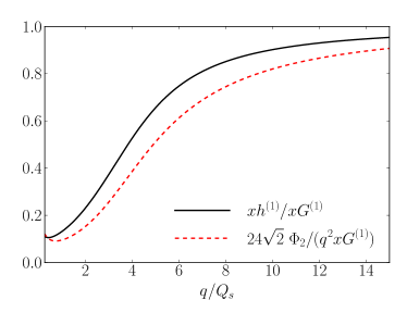
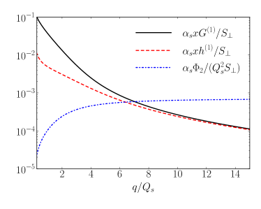
Figure 1: The functions $xG^{(1)}(q^{2})$, $xh^{(1)}(q^{2})$ and $\Phi_{2}(q^{2})$ in the MV model. These functions determine the amplitudes of the $\cos 2n\phi$ contributions to the dijet angular distributions for $n=0$, 1, 2, respectively. See text for details.

Figure 1 shows the functions $xG^{(1)}(q^{2})$, $xh^{(1)}(q^{2})$ and $\Phi_{2}(q^{2})$ in the MV model as written in Eqs. (33,34,41). In the numerical computations we have replaced $1/r^{2}\Lambda^{2}_{\rm IR}\to e+1/r^{2}\Lambda^{2}_{\rm IR}$ in the arguments of the logarithms to ensure that they are $\geq 1$ for all $r^{2}$. Also, we have used $Q_{s}/\Lambda_{\rm IR}=20$.

IV Dijet cross section in DIS

At leading order the cross section for production of a $q\bar{q}$ dijet in DIS is given by Dominguez:2011wm

$$\frac{d\sigma^{\gamma_{T,L}^{\ast}A\rightarrow q\bar{q}X}}{d^{2}k_{1}dz_{1}d^{2}k_{2}dz_{2}} = N_{c}\alpha_{\rm em}e_{q}^{2}\,\delta(p^{+}-k_{1}^{+}-k_{2}^{+})\int\frac{\text{d}^{2}u}{(2\pi)^{2}}\frac{\text{d}^{2}u^{\prime}}{(2\pi)^{2}}\frac{\text{d}^{2}v}{(2\pi)^{2}}\frac{\text{d}^{2}v^{\prime}}{(2\pi)^{2}}$$ (42)

$$\times e^{-iP\cdot(u-u^{\prime})-iq\cdot(v-v^{\prime})}{\cal Q}(u,u^{\prime},v,v^{\prime})\sum_{\lambda\alpha\beta}\psi_{\alpha\beta}^{T,L\lambda}(u)\,\psi_{\alpha\beta}^{T,L\lambda*}(u^{\prime})~{}.$$

$k_{1}$ and $k_{2}$ denote the 2d transverse momenta of the quark and anti-quark, respectively, and $P=(k_{1}-k_{2})/2$, $q=k_{1}+k_{2}$. We assume here that only the dijet is being detected while the azimuthal angle of the electron is integrated over. If the azimuthal angle of the electron can be measured then the dijet cross section could exhibit a more involved angular dependence Pisano:2013cya .

In the “correlation limit” of roughly back to back jets $P^{2}\gg q^{2}$. Using the $\gamma^{*}\to q\bar{q}$ splitting functions from the literature, e.g. Ref. Dominguez:2011wm , and expanding ${\cal Q}$ to fourth order in $u$ or $u^{\prime}$ we obtain

$$\frac{d\sigma^{\gamma_{T}^{\ast}A\rightarrow q\bar{q}X}}{d^{2}k_{1}dz_{1}d^{2}k_{2}dz_{2}}$$

$$~{}~{}~{}~{}~{}=2N_{c}\alpha_{em}e_{q}^{2}\,(2\pi)^{2}\delta(x_{\gamma}-z_{1}-z_{2})\left(z_{2}^{2}+z_{1}^{2}\right)\int\frac{\text{d}^{2}u}{(2\pi)^{2}}\frac{\text{d}^{2}u^{\prime}}{(2\pi)^{2}}\;e^{-iP\cdot(u-u^{\prime})}\nabla K_{0}(\epsilon_{f}u)\cdot\nabla K_{0}(\epsilon_{f}u^{\prime})$$

$$~{}~{}~{}~{}~{}~{}~{}~{}~{}\times\left[u_{i}u_{j}^{\prime}{\cal G}^{i,j}(q)+u_{i}u_{j}^{\prime}u_{k}^{\prime}u_{l}^{\prime}{\cal G}^{i,jkl}(q)+u_{i}u_{j}u_{k}u_{l}^{\prime}{\cal G}^{ijk,l}(q)+u_{i}u_{j}u_{k}^{\prime}u_{l}^{\prime}{\cal G}^{ij,kl}(q)\right]\ ,$$ (43)

$$\frac{d\sigma^{\gamma_{L}^{\ast}A\rightarrow q\bar{q}X}}{d^{2}k_{1}dz_{1}d^{2}k_{2}dz_{2}}=8N_{c}\alpha_{em}e_{q}^{2}\,(2\pi)^{2}\delta(x_{\gamma}-z_{1}-z_{2})z_{1}z_{2}\epsilon_{f}^{2}\int\frac{\text{d}^{2}u}{(2\pi)^{2}}\frac{\text{d}^{2}u^{\prime}}{(2\pi)^{2}}\;e^{-iP\cdot(u-u^{\prime})}K_{0}(\epsilon_{f}u)K_{0}(\epsilon_{f}u^{\prime})$$

$$~{}~{}~{}~{}~{}~{}~{}~{}~{}\times\left[u_{i}u_{j}^{\prime}{\cal G}^{i,j}(q)+u_{i}u_{j}^{\prime}u_{k}^{\prime}u_{l}^{\prime}{\cal G}^{i,jkl}(q)+u_{i}u_{j}u_{k}u_{l}^{\prime}{\cal G}^{ijk,l}(q)+u_{i}u_{j}u_{k}^{\prime}u_{l}^{\prime}{\cal G}^{ij,kl}(q)\right]~{}.$$ (44)

Here, $\epsilon_{f}^{2}=z_{1}z_{2}Q^{2}$ with $Q^{2}$ the virtuality of the photon which is on the order of $P^{2}$.

The integrals over $u$ and $u^{\prime}$ can be performed using the formulas collected in appendix A. The leading (in powers of $1/P^{2}$) contributions proportional to $\cos 2n\phi$, for $n=0$, 1, 2, can be summarized as

$$\frac{d\sigma^{\gamma_{T}^{\ast}A\rightarrow q\bar{q}X}}{d^{2}k_{1}dz_{1}d^{2}k_{2}dz_{2}}$$

$$~{}~{}~{}~{}~{}=\alpha_{s}\alpha_{em}e_{q}^{2}\delta(x_{\gamma}-z_{1}-z_{2})\left(z_{1}^{2}+z_{2}^{2}\right)\left[\frac{P^{4}+\epsilon_{f}^{4}}{(P^{2}+\epsilon_{f}^{2})^{4}}\left(xG^{(1)}(x,q^{2})-\frac{2\epsilon_{f}^{2}P^{2}}{P^{4}+\epsilon_{f}^{4}}xh^{(1)}(x,q^{2})\cos 2\phi+{\cal O}\left(\frac{1}{P^{2}}\right)\right)\right.$$

$$\left.\hskip 199.16928pt-\frac{48\epsilon_{f}^{2}P^{4}}{\sqrt{2}\,(P^{2}+\epsilon_{f}^{2})^{6}}\Phi_{2}(x,q^{2})\cos 4\phi\right]$$ (45)

$$\frac{d\sigma^{\gamma_{L}^{\ast}A\rightarrow q\bar{q}X}}{d^{2}k_{1}dz_{1}d^{2}k_{2}dz_{2}}$$

$$~{}~{}~{}~{}~{}=8\alpha_{s}\alpha_{em}e_{q}^{2}\delta(x_{\gamma}-z_{1}-z_{2})z_{1}z_{2}\epsilon_{f}^{2}\left[\frac{P^{2}}{(P^{2}+\epsilon_{f}^{2})^{4}}\left(xG^{(1)}(x,q^{2})+xh^{(1)}(x,q^{2})\cos 2\phi+{\cal O}\left(\frac{1}{P^{2}}\right)\right)\right.$$

$$\left.\hskip 199.16928pt+\frac{48P^{4}}{\sqrt{2}\,(P^{2}+\epsilon_{f}^{2})^{6}}\Phi_{2}(x,q^{2})\cos 4\phi\right]~{}.$$ (46)

Here, $\cos\phi=\hat{q}\cdot\hat{P}$. Note that the contribution $\sim\cos 4\phi$ is suppressed by $1/P^{2}$ relative to the isotropic and $\sim\cos 2\phi$ pieces which are due to the $xG^{(1)}(x,q^{2})$ and $xh^{(1)}(x,q^{2})$ TMDs.

Figure 2: $\left<\cos 2\phi\right>$ and $\left<\cos 4\phi\right>$ in $\gamma_{L}^{*}+A\to q+\bar{q}$ dijet production from the MV model. See text for details.

Finally, we evaluate numerically the following angular averages for a longitudinally polarized photon:

$$\left<\cos 2\phi\right>=\frac{1}{2}\frac{xh^{(1)}(q^{2})}{xG^{(1)}(q^{2})}~{}~{}~{},~{}~{}~{}\left<\cos 4\phi\right>=\frac{24}{\sqrt{2}\,P^{2}}\left(\frac{P^{2}}{P^{2}+\epsilon_{f}^{2}}\right)^{2}\frac{\Phi_{2}(q^{2})}{xG^{(1)}(q^{2})}~{}.$$ (47)

We employ the MV model expressions for $xG^{(1)}(q^{2})$, $xh^{(1)}(q^{2})$, and $\Phi_{2}(q^{2})$ derived in the previous section. The results are shown in Fig. 2 assuming $\surd P^{2}=4.5\,Q_{s}$, $z=0.5$ and $Q^{2}=P^{2}$. They confirm that for $q^{2}\ll P^{2}$ the average $\cos 4\phi$ is substantially less than the average $\cos 2\phi$ although it may be measurable at a future high-energy electron-ion collider. For more quantitative estimates it is required, however, to account for small-$x$ QCD evolution of these functions. This has been done in Ref. Dumitru:2015gaa for $xG^{(1)}(x,q^{2})$ and $xh^{(1)}(x,q^{2})$ and needs to be extended to $\Phi_{2}(x,q^{2})$.

V Summary

In this paper we have considered the expansion of the quadrupole operator

$$S^{(4)}(x_{1},x_{2};x_{2}^{\prime},x_{1}^{\prime})\equiv\frac{1}{N_{c}}\left<{\rm Tr}\,V^{\dagger}(x_{2})V(x_{1})V^{\dagger}(x_{1}^{\prime})V(x_{2}^{\prime})\right>$$ (48)

about the coincidence limits $u\equiv x_{1}-x_{2}\to 0$, $u^{\prime}\equiv x_{1}^{\prime}-x_{2}^{\prime}\to 0$. At quadratic order it becomes a two-point correlator of light-cone gauge fields DQXY ,

$$u_{i}u^{\prime}_{j}\,\left<{\rm Tr}\,\left[V^{\dagger}({v})\,\frac{i}{g}\partial^{i}V({v})\right]\;\left[V^{\dagger}({v}^{\prime})\,\frac{i}{g}\partial^{j}V({v}^{\prime})\right]\right>$$ (49)

which defines the Weizsäcker-Williams and linearly polarized gluon distributions. We have extended the expansion to fourth order in $u/u^{\prime}$ which leads to more involved correlators of Wilson lines and their derivatives, c.f. Eqs. (9,10,11). Furthermore, we have obtained explicit analytic expressions in a Gaussian, large $N_{c}$ approximation for the specific correlation function denoted as $\Phi_{2}(x,q^{2})$. This function gives rise to a $\sim\cos 4\phi$ azimuthal harmonic in dijet production. First qualitative estimates obtained within a specific Gaussian model (McLerran-Venugopalan model McLerran:1993ni ) indicate that $\langle\cos 4\phi\rangle$ is much smaller than $\langle\cos 2\phi\rangle$ generated by the distribution of linearly polarized gluons $xh^{(1)}(x,q^{2})$, at least in the nearly back to back “correlation limit” $P^{2}\gg q^{2}$.

Appendix A Useful Integrals

We start from the well known integral

$$\int\frac{d^{2}u}{(2\pi)^{2}}\exp(-iu\cdot P)K_{0}(\epsilon_{f}u)=\frac{1}{2\pi}\frac{1}{P^{2}+\epsilon_{f}^{2}}~{}.$$ (50)

Taking a derivative with respect to $P_{i}$ gives

$$\int\frac{d^{2}u}{(2\pi)^{2}}\exp(-iu\cdot P)u_{i}K_{0}(\epsilon_{f}u)=\frac{1}{2\pi i}\frac{2P_{i}}{(P^{2}+\epsilon_{f}^{2})^{2}}~{}.$$ (51)

Repeating this procedure one finds

$$\int\frac{d^{2}u}{(2\pi)^{2}}\exp(-iu\cdot P)u_{i}u_{j}K_{0}(\epsilon_{f}u)=\frac{1}{2\pi}\frac{2}{(P^{2}+\epsilon_{f}^{2})^{2}}\left[\delta_{ij}-\frac{4P_{i}P_{j}}{P^{2}+\epsilon_{f}^{2}}\right]$$ (52)

and

$$\int\frac{d^{2}u}{(2\pi)^{2}}\exp(-iu\cdot P)u_{i}u_{j}u_{k}K_{0}(\epsilon_{f}u)=\frac{1}{2\pi i}\frac{8}{(P^{2}+\epsilon_{f}^{2})^{3}}\left[P_{i}{\delta}_{jk}+P_{j}{\delta}_{ik}+P_{k}{\delta}_{ij}-\frac{6P_{i}P_{j}P_{k}}{P^{2}+\epsilon_{f}^{2}}\right]~{}.$$ (53)

For transverse photon polarization we need

$$\int\frac{d^{2}u}{(2\pi)^{2}}\exp(-iu\cdot P)\frac{\partial}{\partial u_{l}}K_{0}(\epsilon_{f}u) = -\int\frac{d^{2}u}{(2\pi)^{2}}\left(\frac{\partial}{\partial u_{l}}\exp(-iu\cdot P)\right)K_{0}(\epsilon_{f}u)=-\frac{1}{2\pi i}\frac{P_{l}}{P^{2}+\epsilon_{f}^{2}}~{},$$ (54)

$$\int\frac{d^{2}u}{(2\pi)^{2}}\exp(-iu\cdot P)u_{i}\frac{\partial}{\partial u_{l}}K_{0}(\epsilon_{f}u) = -\frac{1}{2\pi}\frac{1}{P^{2}+\epsilon_{f}^{2}}\left({\delta}_{il}-\frac{2P_{i}P_{l}}{P^{2}+\epsilon_{f}^{2}}\right)~{},$$ (55)

$$\int\frac{d^{2}u}{(2\pi)^{2}}\exp(-iu\cdot P)u_{i}u_{j}\frac{\partial}{\partial u_{l}}K_{0}(\epsilon_{f}u) = -\frac{1}{2\pi i}\frac{2}{(P^{2}+\epsilon_{f}^{2})^{2}}\left(\delta_{ij}P_{l}+{\delta}_{il}P_{j}+{\delta}_{jl}P_{i}-\frac{4P_{l}P_{i}P_{j}}{P^{2}+\epsilon_{f}^{2}}\right)~{},$$ (56)

$$\int\frac{d^{2}u}{(2\pi)^{2}}\exp(-iu\cdot P)u_{i}u_{j}u_{k}\frac{\partial}{\partial u_{l}}K_{0}(\epsilon_{f}u) = -\frac{1}{2\pi}\frac{2}{(P^{2}+\epsilon_{f}^{2})^{2}}$$ (57)

$$\times\left(\delta_{il}\delta_{jk}+\delta_{ij}\delta_{kl}+\delta_{ik}\delta_{jl}-4\frac{P_{j}P_{k}\delta_{il}+P_{l}P_{k}\delta_{ij}+P_{i}P_{k}\delta_{jl}+P_{j}P_{l}\delta_{ik}+P_{i}P_{j}\delta_{lk}+P_{i}P_{l}\delta_{jk}}{P^{2}+\epsilon_{f}^{2}}+24\frac{P_{i}P_{j}P_{l}P_{k}}{(P^{2}+\epsilon_{f}^{2})^{2}}\right)$$

Appendix B Power corrections to the isotropic and $\cos 2\phi$ contributions

In this appendix we derive the leading power corrections to the isotropic and $\sim\cos 2\phi$ contributions in Eqs. (45, 46). These are suppressed by one power of $P^{2}$ but logarithmically enhanced by a factor of $\log P^{2}/\Lambda^{2}$, and arise from the terms in the expansion of the quadrupole ${\cal Q}^{G}$ in (35) which involve $\Gamma(u^{2})$ or $\Gamma(u^{\prime 2})$.

First we write

$$\Gamma(u^{2})=u^{2}\hat{\Gamma}(u^{2})~{}~{}~{}~{},~{}~{}~{}~{}\hat{\Gamma}(u^{2})=\frac{Q_{s}^{2}}{4C_{F}}\log\frac{1}{u^{2}\Lambda^{2}}~{}.$$ (58)

The prefactor of the logarithm in $\hat{\Gamma}(u^{2})$ is specific to the MV model but $\hat{\Gamma}(u^{2})\sim\log{1}/{u^{2}\Lambda^{2}}$ applies at small $u$ even when the gluon distribution acquires an anomalous dimension.

Now we extend the expansion about small $u$, $u^{\prime}$ from Eqs. (5, 45, 46) as follows:

$$u_{i}u_{j}^{\prime}{\cal G}^{i,j}(q)$$

$$+u_{i}u_{j}^{\prime}u_{k}^{\prime}u_{l}^{\prime}\log\frac{1}{u^{\prime 2}\Lambda^{2}}{\cal G}^{i,jkl}_{\text{log}}(q)+u_{i}u_{j}u_{k}u_{l}^{\prime}\log\frac{1}{u^{2}\Lambda^{2}}{\cal G}^{ijk,l}_{\text{log}}(q)+u_{i}u_{j}u_{k}^{\prime}u_{l}^{\prime}\log\frac{1}{u^{\prime 2}\Lambda^{2}}\log\frac{1}{u^{2}\Lambda^{2}}{\cal G}^{ij,kl}_{\text{log}}(q)~{}.$$ (59)

Here, we have only listed the leading power and the log-enhanced power corrections. From Eq. (35) one can read off

$${\cal G}^{i,jkl}_{\text{log}}(r) = \frac{Q_{s}^{2}}{4C_{F}}\left(1-\left[S^{(2)}(r^{2})\right]^{2}-C_{F}\Gamma(r^{2})\right)\delta^{kl}\frac{\delta^{ij}\Gamma^{(1)}(r^{2})+2r^{i}r^{j}\Gamma^{(2)}(r^{2})}{2\Gamma^{2}(r^{2})}~{},$$ (60)

$${\cal G}^{ijk,l}_{\text{log}}(r) = \frac{Q_{s}^{2}}{4C_{F}}\left(1-\left[S^{(2)}(r^{2})\right]^{2}-C_{F}\Gamma(r^{2})\right)\delta^{jk}\frac{\delta^{il}\Gamma^{(1)}(r^{2})+2r^{i}r^{l}\Gamma^{(2)}(r^{2})}{2\Gamma^{2}(r^{2})}~{},$$ (61)

$${\cal G}^{ij,kl}_{\text{log}}(r) = \frac{1}{4}\delta^{ij}\delta^{kl}C_{F}^{2}\left(\frac{Q_{s}^{2}}{4C_{F}}\right)^{2}~{}.$$ (62)

We now perform the integrals over $u$ and $u^{\prime}$ written in Eqs. (45, 46) using the formulas given in appendix A. For the terms involving logarithms those expressions have to be multiplied by $\log 1/u^{2}\Lambda^{2}$ with $1/u$ replaced by $(P^{2}+\epsilon_{f}^{2})/\epsilon_{f}$ (in the leading $\log P/\Lambda$ approximation). The final step is to perform a Fourier transform w.r.t. $r=v-v^{\prime}$, which is conjugate to $q$, and an integration over $(v+v^{\prime})/2$, which gives a factor of transverse area. We then find that in Eq. (45) we have to replace

$$xG^{(1)}(x,q^{2}) \to xG^{(1)}(x,q^{2})-Q_{s}^{2}\frac{\epsilon_{f}^{2}\left((P^{2}-\epsilon_{f}^{2})^{2}+2P^{4}\right)}{\left(P^{2}+\epsilon_{f}^{2}\right)^{2}(P^{4}+\epsilon_{f}^{4})}\log\left(\frac{P^{2}+\epsilon_{f}^{2}}{\Lambda\epsilon_{f}}\right)x\tilde{G}^{(1)}(x,q^{2})~{},$$ (63)

$$xh^{(1)}(x,q^{2}) \to xh^{(1)}(x,q^{2})-Q_{s}^{2}\frac{2\epsilon_{f}^{2}-P^{2}}{\left(P^{2}+\epsilon_{f}^{2}\right)^{2}}\log\left(\frac{P^{2}+\epsilon_{f}^{2}}{\Lambda\epsilon_{f}}\right)x\tilde{h}^{(1)}(x,q^{2})~{}.$$ (64)

Similarly, in Eq. (46),

$$xG^{(1)}(x,q^{2}) \to xG^{(1)}(x,q^{2})-2Q_{s}^{2}\frac{2\epsilon_{f}^{2}-P^{2}}{\left(P^{2}+\epsilon_{f}^{2}\right)^{2}}\log\left(\frac{P^{2}+\epsilon_{f}^{2}}{\Lambda\epsilon_{f}}\right)x\tilde{G}^{(1)}(x,q^{2})~{},$$ (65)

$$xh^{(1)}(x,q^{2}) \to xh^{(1)}(x,q^{2})-2Q_{s}^{2}\frac{2\epsilon_{f}^{2}-P^{2}}{\left(P^{2}+\epsilon_{f}^{2}\right)^{2}}\log\left(\frac{P^{2}+\epsilon_{f}^{2}}{\Lambda\epsilon_{f}}\right)x\tilde{h}^{(1)}(x,q^{2})~{},$$ (66)

with

$$x\tilde{G}^{(1)}(x,q^{2}) = \frac{8N_{c}}{\alpha_{s}}\frac{S_{\perp}}{(2\pi)^{2}}\int\frac{d^{2}r}{(2\pi)^{2}}e^{-iq\cdot r}\left(C_{F}\Gamma(r^{2})+\left[S^{(2)}(r^{2})\right]^{2}-1\right)\frac{\Gamma^{(1)}(r^{2})+r^{2}\Gamma^{(2)}(r^{2})}{C_{F}\Gamma^{2}(r^{2})}$$ (67)

$$x\tilde{h}^{(1)}(x,q^{2}) = \frac{8N_{c}}{\alpha_{s}}\frac{S_{\perp}}{(2\pi)^{2}}\int\frac{d^{2}r}{(2\pi)^{2}}e^{-iq\cdot r}\cos(2\phi_{r})\left(C_{F}\Gamma(r^{2})+\left[S^{(2)}(r^{2})\right]^{2}-1\right)\frac{r^{2}\Gamma^{(2)}(r^{2})}{C_{F}\Gamma^{2}(r^{2})}~{}.$$ (68)

At high transverse momentum, $q^{2}\gg Q_{s}^{2}$, the functions $x\tilde{G}^{(1)}(x,q^{2})$ and $x\tilde{h}^{(1)}(x,q^{2})$ approach $xG^{(1)}(x,q^{2})$ and $xh^{(1)}(x,q^{2})$, respectively. In that limit, the corrections in Eqs. (63, 64, 65, 66) are of order $(Q_{s}^{2}/P^{2})\,\log P^{2}/\Lambda^{2}$. Assuming, for example, $P^{2}/10=\epsilon_{f}^{2}/10=20\Lambda^{2}=q^{2}=Q_{s}^{2}$ leads to corrections of about 8% for transverse polarization, and twice that for a longitudinal photon.

For comparison, the power correction that generates the $\sim\cos 4\phi$ contribution in Eqs. (45, 46) is of order $q^{2}/P^{2}$. To see this, write $\tilde{\Phi}_{2}(x,q^{2})=\Phi_{2}(x,q^{2})/q^{2}$; this function has the same dimension and the same $\sim 1/q^{2}$ fall off at high transverse momentum as $xG^{(1)}(x,q^{2})$ and $xh^{(1)}(x,q^{2})$. Its prefactor in Eqs. (45, 46) is then suppressed by one power of $q^{2}/P^{2}$ as compared to the prefactors of $xG^{(1)}(x,q^{2})$ and $xh^{(1)}(x,q^{2})$.

References

(1)
F. Dominguez, C. Marquet, B. W. Xiao and F. Yuan,
Phys. Rev. D 83, 105005 (2011)
[arXiv:1101.0715 [hep-ph]].
(2)
R. Angeles-Martinez et al.,
Acta Phys. Polon. B 46, no. 12, 2501 (2015)
[arXiv:1507.05267 [hep-ph]].
(3)
P. J. Mulders and J. Rodrigues,
Phys. Rev. D 63, 094021 (2001)
[hep-ph/0009343].
(4)
S. Meissner, A. Metz and K. Goeke,
Phys. Rev. D 76, 034002 (2007)
[hep-ph/0703176 [HEP-PH]].
(5)
D. Boer, P. J. Mulders and C. Pisano,
Phys. Rev. D 80, 094017 (2009)
[arXiv:0909.4652 [hep-ph]].
(6)
A. Metz and J. Zhou,
Phys. Rev. D 84, 051503 (2011)
[arXiv:1105.1991 [hep-ph]].
(7)
F. Dominguez, J. W. Qiu, B. W. Xiao and F. Yuan,
Phys. Rev. D 85, 045003 (2012)
[arXiv:1109.6293 [hep-ph]].
(8)
D. Boer, S. J. Brodsky, P. J. Mulders and C. Pisano,
Phys. Rev. Lett. 106, 132001 (2011)
[arXiv:1011.4225 [hep-ph]].
(9)
J. W. Qiu, M. Schlegel and W. Vogelsang,
Phys. Rev. Lett. 107, 062001 (2011)
[arXiv:1103.3861 [hep-ph]].
(10)
A. Dumitru, T. Lappi and V. Skokov,
Phys. Rev. Lett. 115, no. 25, 252301 (2015)
[arXiv:1508.04438 [hep-ph]].
(11)
D. Boer et al.,
arXiv:1108.1713 [nucl-th];
A. Accardi et al.,
arXiv:1212.1701 [nucl-ex].
(12)
J. Huang and T. Ullrich, priv. communication
(13)
L. D. McLerran and R. Venugopalan,
Phys. Rev. D 49, 2233 (1994)
[hep-ph/9309289];
Phys. Rev. D 49, 3352 (1994)
[hep-ph/9311205].
(14)
E. Iancu, K. Itakura and L. McLerran,
Nucl. Phys. A 724, 181 (2003)
[hep-ph/0212123];
H. Fujii, F. Gelis and R. Venugopalan,
Nucl. Phys. A 780, 146 (2006)
[hep-ph/0603099];
C. Marquet and H. Weigert,
Nucl. Phys. A 843, 68 (2010)
[arXiv:1003.0813 [hep-ph]];
E. Iancu and D. N. Triantafyllopoulos,
JHEP 1111, 105 (2011)
[arXiv:1109.0302 [hep-ph]];
JHEP 1204, 025 (2012)
[arXiv:1112.1104 [hep-ph]];
T. Lappi, B. Schenke, S. Schlichting and R. Venugopalan,
JHEP 1601, 061 (2016)
[arXiv:1509.03499 [hep-ph]].
(15)
A. Kovner and M. Lublinsky,
Phys. Rev. D 84, 094011 (2011)
[arXiv:1109.0347 [hep-ph]].
(16)
A. Dumitru, J. Jalilian-Marian, T. Lappi, B. Schenke and R. Venugopalan,
Phys. Lett. B 706, 219 (2011)
[arXiv:1108.4764 [hep-ph]].
(17)
J. P. Blaizot, F. Gelis and R. Venugopalan,
Nucl. Phys. A 743, 57 (2004)
[hep-ph/0402257].
(18)
C. Pisano, D. Boer, S. J. Brodsky, M. G. A. Buffing and P. J. Mulders,
JHEP 1310, 024 (2013)
[arXiv:1307.3417 [hep-ph]].