Calabi-Yau structures on topological Fukaya categories

Abstract.

We develop a local-to-global formalism for constructing Calabi-Yau structures for global sections of constructible sheaves or cosheaves of categories. The required data — a morphism between the sheafified Hochschild homology with the topological dualizing sheaf, satisfying a nondegeneracy condition — specializes to the classical notion of orientation when applied to the category of local systems on a manifold. We apply this construction to the cosheaves on arboreal skeleta arising in the microlocal approach to the A-model.

1. Introduction

A compact complex manifold with trivial canonical bundle is said to be Calabi-Yau. On such a manifold, Serre duality takes the simple form $\operatorname{Hom}(E,F)\cong\operatorname{Hom}(F,E)^{*}[d]$. This is a categorical analogue of nondegenerate trace on an algebra, and there is an associated notion of Calabi-Yau category, generalizing the notion of Frobenius algebra.

Such categories are precisely the categories of boundary conditions in two dimensional topological field theories, from which these theories may be reconstructed [18, 60]. In particular, much of the relationship between the topological A-model and B-model is captured by an equivalence between the Fukaya category of Lagrangians on a symplectic manifold, and the category of coherent sheaves on the mirror algebraic variety, these being the categories of boundary conditions of open strings in the respective theories [51]. Moreover, other invariants associated to these theories should in principle be computable from the Calabi-Yau categories, in particular the partition function, i.e. Gromov-Witten type invariants [19], and also BPS counts, i.e. Donaldson-Thomas type invariants [53, 54]. Related considerations show that moduli of objects in CY categories carry shifted symplectic structures and admit quantizations [76, 14, 12].

Our purpose here is to establish a local-to-global formalism for constructing certain Calabi-Yau categories which arise in the topological A-model. That such a local-to-global procedure should exist is strongly suggested by the fact that, on the one hand, certain Fukaya categories should carry Calabi-Yau structures, and on the other, they are known to be equivalent to categories of microlocal sheaves in certain exact situations [73, 67, 34, 35, 83, 72, 36]. This equivalence underlies one approach to homological mirror symmetry [28, 70, 71, 57, 32]. If one wants to e.g. use the ideas of [19] to extract enumerative mirror symmetry from this microlocal sheaf description, it will be necessary to construct Calabi-Yau structures in the microlocal sheaf setting, prove a comparison with [33], and and show that the aforementioned mirror symmetry results respect Calabi-Yau structures. Here we take the first step.

Another motivation is that moduli of microlocal sheaves naturally describe many spaces of interest, for instance: moduli spaces of (possibly irregular) local systems, positroid varieties, multiplicative Nakajima varieties, the A-polynomial of a knot, etc. Many of these spaces are known or expected to carry symplectic structures and quantizations; in light of [76, 14, 12], our work provides a uniform construction of these structures.

The setting for our local-to-global formalism is:

Definition 1.1.

A constructibly cosheaved in categories (ccc) space is a pair $(X,\mathcal{F})$ where $X$ is a topological space and $\mathcal{F}$ is a cosheaf on $X$ valued in the $\infty$-category of small dg categories, constructible with respect to some finite stratification of $X$.

We define analogously the notion of constructibly sheaved in categories (csc) space $(X,\mathcal{F})$.

Given a ccc or csc space as above, we say that a map $X\to Y$ or $Y\to X$ is constructible if it is stratifiable by a finite stratification with respect to which $\mathcal{F}$ is constructible. In particular we say $U\subset X$ is constructible if it is a union of strata for some finite stratification of $X$ with respect to which $\mathcal{F}$ is constructible.

Example.

Let $M$ be a manifold (or sufficiently reasonable topological space) and $k$ a field. Let $Loc(M)$ be the category of (unbounded, possibly infinite rank) local systems on $M$, valued in the category of perfect $k$-modules. Then $U\mapsto Loc(U)$, together the evident restriction maps, determines a sheaf $\mathcal{L}oc$ on $M$ valued in the category of presentable dg categories with limit-preserving morphisms. Taking adjoints gives a cosheaf, also denoted $\mathcal{L}oc$, on $M$, valued in the category of presentable dg categories with colimit-preserving morphisms.

Let $Loc^{b}(U)\subset Loc(U)$ be the full subcategory of local systems of perfect $k$-modules, and $\mathcal{L}oc^{b}\subset\mathcal{L}oc$ the corresponding full subsheaf. Then $(M,\mathcal{L}oc^{b})$ is a csc space.

Let $Loc^{c}(U)\subset Loc(U)$ be the full subcategory of compact objects, and $\mathcal{L}oc^{c}\subset\mathcal{L}oc$ the corresponding full subcosheaf. Then $(M,\mathcal{L}oc^{c})$ is a ccc space.

The cospecialization maps of the cosheaf $\mathcal{L}oc^{c}$ are nontrivial to describe, being the analogue in sheaf theory of wrapping in the Fukaya category [70, 36].

Example.

There are evident isomorphisms $Loc(S^{1})=\operatorname{Mod}\,k[t,t^{-1}]$ and $Loc^{c}(S^{1})=\operatorname{Perf}\,k[t,t^{-1}]$. The category $Loc^{b}(S^{1})$ is the finite $k$-rank modules for $k[t,t^{-1}]$. Note that it is possible to recover $Loc^{b}$ from $Loc^{c}$ but not vice versa. This phenomenon is what forces us to consider the cosheaves.

More generally, microlocal sheaf theory provides the structure of a csc [55] and ccc [70] space to any (singular) subanalytic Legendrian in a cosphere bundle, $X\subset S^{*}M$. More generally, one can do with only the germ of an embedding into some contact manifold, plus some topological ‘Maslov’ data [83, 72]. We briefly recall this in Section 6.

For Legendrians $X$ with a certain prescribed set of ‘arboreal’ singularities, Nadler showed in [68] that the local categories can be described combinatorially; in Section 4 we turn this into a definition to give a construction of some ccc spaces which should be intelligible to a reader innocent of microlocal sheaf theory and symplectic geometry.

Given a ccc or csc space $(X,\mathcal{F})$, we are interested in how to construct Calabi-Yau structures on $\mathcal{F}(X)$ from local data on $X$. In fact the situation is rather different for sheaves and cosheaves, for the following reason. There are two notions of Calabi-Yau structure, one appropriate to proper (i.e. hom-finite) categories, and another appropriate to smooth (i.e. perfect diagonal) categories, which coincide for smooth and proper (aka saturated) categories. Since hom-finiteness is preserved under homotopy finite limits, it is natural to consider constructible sheaves of proper categories; similarly, smoothness is preserved under homotopy finite colimits and so it is natural to consider constructible cosheaves of smooth categories.

Example.

For any manifold $M$, the category $Loc^{b}(M)$ is proper and the category $Loc^{c}(M)$ is smooth. For $S^{1}$, the category $Loc^{b}(S^{1})$ is not smooth, and the category $Loc^{c}(S^{1})$ is not proper.

The situation for sheaves of proper categories is simpler, so we consider it first. Recall that a proper Calabi-Yau structure of degree $d$ on a category $\mathcal{C}$ is roughly a system of isomorphisms $\mathcal{C}(x,y)\simeq\mathcal{C}(y,x)^{*}[-d]$. Because the Hochschild complex presents the (derived) tensor product of the diagonal bimodule of $\mathcal{C}$ with itself, such a structure can be specified by a function on the Hochschild complex, $\mathrm{HH}(\mathcal{C})\to k[-d]$. In fact one demands this factor through the map to homotopy $S^{1}$-coinvariants (orbits) $\mathrm{HH}(\mathcal{C})\to\mathrm{HH}(\mathcal{C})_{S^{1}}$. This is because the Hochschild complex is the state space associated to the circle, from the point of view of topological field theory, and one must work equivariantly with respect to this circle action.

Hochschild homology is functorial, so $U\mapsto\mathrm{HH}(\mathcal{F}(U))$ determines a presheaf. We understand this presheaf as taking values in the dg category of chain complexes localized along quasi-isomorphisms. The presheaf $U\mapsto\mathrm{HH}(\mathcal{F}(U))$ is not generally a sheaf.

Example.

$\mathrm{HH}(\mathcal{L}oc^{b}(U))$ can be identified with $k$-valued cochains on the free loop space of $U$. (For further discussion see Sec. 3.1.1)

We form the sheafification $\mathcal{H}\mathcal{H}(\mathcal{F})$ of this presheaf; the resulting sheaf carries a suitable $S^{1}$ action inherited from the local $S^{1}$ actions.

Example.

$\mathcal{H}\mathcal{H}(\mathcal{L}oc^{b})$ is the constant sheaf with stalk $k$, and the $S^{1}$ action is trivial.

We then seek a local construction of a morphism $\mathcal{H}\mathcal{H}(\mathcal{F})(X)_{S^{1}}\to k[-d]$. By composition with the natural morphism $\mathrm{HH}(\mathcal{F}(X))\to\mathcal{H}\mathcal{H}(\mathcal{F})(X)_{S^{1}}$, such a morphism would determine a function on the Hochschild complex.

For any sheaf $\mathcal{G}$, the local data which would produce a map $\mathcal{G}(X)\to k[-d]$ is nothing other than a morphism $\mathcal{G}\to\omega_{X}[-d]$, the latter being the Verdier dualizing sheaf. When $\mathcal{G}=\mathcal{H}\mathcal{H}(\mathcal{F})$, it is possible to formulate a local version of the condition that the resulting trace induces a perfect pairing. This is because for an open subset $U\subset X$, and objects $x,y\in\mathcal{F}(U)$, there is a constructible sheaf $\mathcal{F}|_{U}^{x,y}$ of morphisms on $U$. That is, for $V\subset U$ we have $\mathcal{F}|_{U}^{x,y}(V)=\mathcal{H}om_{\mathcal{F}(V)}(x|_{V},y|_{V})$.

Definition 1.2.

Let $(X,\mathcal{F})$ be a csc space. A morphism $\Omega:\mathcal{H}\mathcal{H}(\mathcal{F})_{S^{1}}\to\omega_{X}[-d]$ is an orientation (of degree $d$) if for any $U$ and pair $x,y\in\mathcal{F}(U)$, the induced morphism

$$\tilde{\Omega}:\mathcal{F}|_{U}^{x,y}\to\operatorname{\mathcal{H}\kern-1.2pt\mathit{om}}_{U}(\mathcal{F}|_{U}^{y,x},\omega_{U})[-d]$$

is an isomorphism.

If $(X,\mathcal{F})$ admits an orientation, we say it is orientable; in this case it follows from the nondegeneracy condition that $\mathcal{F}(U)$ is proper for any constructible $U$.

Example.

We have $\mathcal{H}\mathcal{H}(\mathcal{L}oc^{b})=k_{M}$, with the trivial $S^{1}$-action. If $M$ is a manifold, an orientation of $(M,\mathcal{L}oc^{b})$ is thus a choice of isomorphism $k_{M}\simeq\omega_{M}[-\dim M]$, i.e., an orientation of $M$ in the sense of classical topology.

Example.

(Prop 3.5) A csc space over $(\mathrm{point},\mathcal{F})$ amounts to just a single category $\mathcal{F}(\mathrm{point})$. An orientation of $(\mathrm{point},\mathcal{F})$ in the sense of Definition 1.6 is just a proper Calabi-Yau structure on $\mathcal{F}(\mathrm{point})$.

Example.

(Prop 3.6) Consider a csc space $([0,1),\mathcal{F})$, where $\mathcal{F}$ is constructible with respect to the stratification $[0,1)=\{0\}\cup(0,1)$. Then an orientation of $([0,1),\mathcal{F})$ is equivalent to a right (aka proper) Calabi-Yau structure on the morphism $\mathcal{F}([0,1))\to\mathcal{F}((0,1))$ in the sense of Brav and Dyckherhoff [12].

Given a continuous map $f:X\to Y$ we may pushforward sheaves of categories by the usual formula $f_{*}\mathcal{F}(U)=\mathcal{F}(f^{-1}(U))$. There is a natural morphism $\mathcal{H}\mathcal{H}(f_{*}\mathcal{F})\to f_{*}\mathcal{H}\mathcal{H}(\mathcal{F})$. There is also a natural morphism $f_{!}\omega_{X}=f_{!}f^{!}\omega_{Y}\to\omega_{Y}$. Thus if $f$ is proper (so $f_{*}=f_{!}$), an orientation on $X$ determines the composition

$$\mathcal{H}\mathcal{H}(f_{*}\mathcal{F})\to f_{*}\mathcal{H}\mathcal{H}(\mathcal{F})\xrightarrow{\Omega}f_{*}\omega_{X}\to\omega_{Y},$$

which we denote as $f_{*}\Omega$.

Theorem 1.3.

(Thm. 3.7) Let $(X,\mathcal{F})$ be a csc space, and $f:X\to Y$ be proper and constructible. If $\Omega$ orients $(X,\mathcal{F})$, then $f_{*}\Omega$ orients $(Y,f_{*}\mathcal{F})$.

The proof of Theorem 1.3, along with some further discussion of the above examples, can be found in Section 3.2.

Corollary 1.4.

If $(X,\mathcal{F})$ is a csc space and $X$ is compact, then an orientation of $(X,\mathcal{F})$ induces a proper Calabi-Yau structure on $\mathcal{F}(X)$.

Corollary 1.5.

Suppose $X=X_{0}\cup_{\partial X_{0}}(\partial X_{0}\times[0,1))$ where $X_{0}$ is compact. Suppose $(X,\mathcal{F})$ is a csc space and $\mathcal{F}$ is stratifiable with respect to some stratification which, on $\partial X_{0}\times[0,1)$, is the product of a stratification on $\partial X_{0}$ and the stratification $[0,1)=\{0\}\cup(0,1)$.

Then an orientation of $(X,\mathcal{F})$ induces a right (aka proper) Calabi-Yau structure on the map $\mathcal{F}(X)\to\mathcal{F}(\partial X_{0}\times(0,1))$.

Proof.

Push forward along the map $X\to[0,1)$ carrying $X_{0}\to 0$ and $\partial X_{0}\times[0,1)\to[0,1)$. ∎

We turn to the setting of ccc spaces. The data of an orientation will be entirely analogous: it is a map of cosheaves $\Omega:\omega_{X}^{\vee}\to\mathcal{H}\mathcal{H}(\mathcal{F})^{S^{1}}[-d]$ from the linear dual of the dualizing sheaf to the cosheafified negative cyclic homology. However, phrasing the nondegeneracy condition is more difficult, essentially because there is no useful analogue of the evaluated-at-objects Hom sheaf $\mathcal{F}^{x,y}$ and instead we must directly with cosheaves of endomorphisms.

In general, categories of endomorphisms of $(\infty,1)$-categories are most naturally viewed and manipulated as $(\infty,2)$-categories; we will use the tools developed in [45, 44].

Starting from a cosheaf of smooth categories $\mathcal{F}$ on some $X$, we produce its associated diagonal cosheaf $\Delta\mathcal{F}$ (Definition 8.22), valued in the category $\operatorname{End}(\operatorname{DGCat})$ of bimodules over dg categories. For any open $U\subset X$, there is an related cosheaf of $\mathcal{F}(U)$-bimodules that we denote $\Delta\!\!\!\!\Delta(\mathcal{F}|_{U})$. We show that a map $\Omega$ as above determines, for each $U$, a morphism of sheaves of bimodules $\Delta\!\!\!\!\Delta(\mathcal{F}|_{U})^{!}\to\mathbb{D}\Delta\!\!\!\!\Delta(\mathcal{F}|_{U})[-d]$ from the left dual to the covariant (Lurie) Verdier dual of $\Delta\!\!\!\!\Delta(\mathcal{F}|_{U})$.

Definition 1.6.

Let $(X,\mathcal{F})$ be a ccc space. A map $\Omega:\omega_{X}^{\vee}\to\mathcal{H}\mathcal{H}(\mathcal{F})^{S^{1}}[-d]$ determines an orientation (of degree $d$) if, for every $U$, the induced morphism $\Delta\!\!\!\!\Delta(\mathcal{F}|_{U})^{!}\to\mathbb{D}\Delta\!\!\!\!\Delta(\mathcal{F}|_{U})[-d]$ is an isomorphism.

In fact, it is enough to check for any collection of $U$ which cover $X$, e.g. the stars of all strata. The nondegeneracy condition implies that $\mathcal{F}(U)$ is smooth for any constructible $U$.

Remark.

Definition 1.2 is equivalent to a formulation in terms of bimodule sheaves parallel to Definition 1.6. The point of Definition 1.2 is that it is much easier than Definition 1.6 to formulate and check.

The properties of orientations on ccc spaces are entirely analogous to orientations on csc spaces.

Example.

We have $\mathcal{H}\mathcal{H}(\mathcal{L}oc^{c})=k_{M}$, the constant cosheaf with the trivial $S^{1}$-action. By contrast $\mathrm{HH}(\mathcal{L}oc^{c}(U))$ is chains on the free loop space of $U$. If $M$ is a manifold, an orientation of $(M,\mathcal{L}oc^{c})$ is an orientation of $M$. This is nontrivial to check directly, but we will shortly give an argument reducing it to the case of $(M,\mathcal{L}oc^{b})$.

Example.

(Prop. 9.6) A ccc space $(\mathrm{point},\mathcal{F})$ amounts to just a single category $\mathcal{F}(\mathrm{point})$. An orientation on $(\mathrm{point},\mathcal{F})$ is just a smooth Calabi-Yau structure on $\mathcal{F}(\mathrm{point})$ in the usual sense.

Example.

(Prop. 9.7) Consider a ccc space $([0,1),\mathcal{F})$, where $\mathcal{F}$ is constructible for $[0,1)=\{0\}\cup(0,1)$. Then an orientation of $([0,1),\mathcal{F})$ is equivalent to a left (aka smooth) Calabi-Yau structure on the morphism $\mathcal{F}((0,1))\to\mathcal{F}([0,1))$ in the sense of Brav and Dyckherhoff [12].

Given a continuous map $f:X\to Y$ we may pushforward cosheaves of categories by the usual formula $f_{*}\mathcal{F}(U)=\mathcal{F}(f^{-1}(U))$. There is a natural morphism $f_{*}\mathcal{H}\mathcal{H}(\mathcal{F})\to\mathcal{H}\mathcal{H}(f_{*}\mathcal{F})$. Thus if $f$ is proper (so $f_{*}=f_{!}$), an orientation of $(X,\mathcal{F})$ determines the composition

$$\omega_{Y}^{\vee}\to f_{*}\omega_{X}^{\vee}\xrightarrow{\Omega}f_{*}\mathcal{H}\mathcal{H}(\mathcal{F})\to\mathcal{H}\mathcal{H}(f_{*}\mathcal{F}),$$

which we denote as $f_{*}\Omega$.

Theorem 1.7.

(Thm. 9.8) Let $(X,\mathcal{F})$ be a ccc space, and $f:X\to Y$ be proper and constructible. If $\Omega$ orients $(X,\mathcal{F})$, then $f_{*}\Omega$ orients $(Y,f_{*}\mathcal{F})$.

Further exposition of the above examples and the proof of Theorem 1.7 can be found in Section 9.2.

Corollary 1.8.

If $(X,\mathcal{F})$ is a ccc space and $X$ is compact, then an orientation of $(X,\mathcal{F})$ induces a smooth Calabi-Yau structure on $\mathcal{F}(X)$.

Corollary 1.9.

Suppose $X=X_{0}\cup_{\partial X_{0}}(\partial X_{0}\times[0,1))$ where $X_{0}$ is compact. Suppose $(X,\mathcal{F})$ is a ccc space and $\mathcal{F}$ is stratifiable with respect to some stratification which, on $\partial X_{0}\times[0,1)$, is the product of a stratification on $\partial X_{0}$ and the stratification $[0,1)=\{0\}\cup(0,1)$.

Then an orientation of $(X,\mathcal{F})$ induces a left (aka smooth) Calabi-Yau structure on the map $\mathcal{F}(X)\to\mathcal{F}(\partial X_{0}\times(0,1))$.

Example.

Suppose $([0,1],\mathcal{F})$ is a ccc space and $\mathcal{F}$ is constructible for $[0,1]=\{0\}\cup(0,1)\cup\{1\}$. Then $\mathcal{F}([0,1))\leftarrow\mathcal{F}((0,1))\rightarrow\mathcal{F}((0,1])$ are both left Calabi-Yau morphisms. Applying Corollary 1.8, we find a Calabi-Yau structure on the pushout, recovering a result of [12].

As we have mentioned, it is difficult to verify directly that a given $\Omega$ in fact determines a smooth Calabi-Yau structure (indeed, it was even difficult to say what this should mean). To deal with this we use a duality between ccc and csc spaces. For a given category $\mathcal{C}$, we write $\mathcal{C}^{pp}=\operatorname{Hom}(\mathcal{C},\operatorname{Perf}(k))$ for its pseudoperfect modules. If $(X,\mathcal{F})$ is a ccc space with a cosheaf of smooth categories, then $(X,\mathcal{F}^{pp})$ is a csc space with a sheaf of proper categories.

In general, smooth CY structures give proper CY structures on the pseudoperfect modules [12]; this sheafifies as:

Proposition 1.10.

(Prop. 9.11) An orientation on a ccc space $(X,\mathcal{F})$ induces an orientation on the csc space $(X,\mathcal{F}^{pp})$.

We would like to have a result in the other direction. In the case where $X$ is a point, one knows what condition to impose: if $\mathcal{C}$ is a smooth and proper category, then there is an equivalence $\mathcal{C}\simeq\mathcal{C}^{pp}$; moreover there is an isomorphism $\mathrm{HH}(\mathcal{C})^{S^{1}}\simeq\operatorname{Hom}_{k}(\mathrm{HH}(\mathcal{C})_{S^{1}},k)$ which gives a bijection between smooth and proper CY structures on $\mathcal{C}$ [12].

The basic problem we encounter when $X$ has nontrivial topology is that the natural morphism $\mathcal{C}\to\operatorname{Hom}(\mathcal{C}^{pp},\operatorname{Perf}(k))$ is not generally an isomorphism. Nevertheless, we have:

Lemma 1.11.

(Lem. 9.14) If $(X,\mathcal{F})$ is a ccc space such that the stalks of $\mathcal{F}$ are smooth and proper, then the cosheaf $\mathcal{H}\mathcal{H}(\mathcal{F})^{S^{1}}$ is the linear dual to the sheaf $\mathcal{H}\mathcal{H}(\mathcal{F}^{pp})_{S^{1}}$.

Theorem 1.12.

(Thm. 9.15) If $(X,\mathcal{F})$ is a ccc space such that the stalks of $\mathcal{F}$ are smooth and proper, then a morphism $\omega_{X}^{\vee}\to\mathcal{H}\mathcal{H}(\mathcal{F})^{S^{1}}[-d]$ determines a smooth Calabi-Yau structure on $(X,\mathcal{F})$ if and only if the dual morphism $\mathcal{H}\mathcal{H}(\mathcal{F}^{pp})_{S^{1}}\to\omega_{X}[-d]$ determines a proper Calabi-Yau structure on $(X,\mathcal{F}^{pp})$.

Example.

The stalk of $\mathcal{L}oc^{c}$ at any point is $\mathrm{Perf}(k)$, so in particular smooth and proper. Note that nevertheless $\mathcal{L}oc^{c}(S^{1})$ is not proper; yet, if the base space $M$ is a manifold, then a choice of orientation gives an orientation of the proper sheaf $\mathcal{L}oc^{b}$, and by the result above, an orientation of the smooth cosheaf $\mathcal{L}oc^{c}$.

We turn to constructions of ccc spaces and orientations. Our main examples are Nadler’s arboreal spaces, which originate in the microlocal sheaf theory, but as ccc spaces are essentially combinatorial in nature: they can be built directly from the representation theory of tree quivers [68]. We systematically adopt here this combinatorial point of view, making explicit in Section 4 the construction of the ccc structure on the arboreal singularities without reference to microlocal sheaf theory. In brief, to a rooted tree $T$ with some marked leaves is attached a certain stratified topological space $\mathbb{T}$ such that each stratum is labelled by a tree and each attaching map is labelled by a correspondence of trees. There is a constructible cosheaf of smooth categories $\mathcal{A}$ on $\mathbb{T}$, whose stalks are quiver representation categories. By construction, the cosheaf $\mathcal{A}_{\mathbb{T}}$ has smooth and proper stalks.

Our main new result regarding the arboreal spaces is:

Theorem 1.13.

(Thm. 5.7) Let $\vv{T}$ be a rooted tree with marked leaves, and $\mathbb{T}$ the corresponding arboreal singularity. The canonical $S^{1}$-action on $\mathcal{H}\mathcal{H}(\mathcal{A})$ is trivial, and there is an isomorphism, unique up to a scalar, $\mathcal{H}\mathcal{H}(\mathcal{A})\cong\omega_{\mathbb{T}}[-\dim\mathbb{T}]$, giving an orientation on the ccc space $(\mathbb{T},\mathcal{A})$.

We define an arboreal space to be a ccc space locally modeled on some $(\mathbb{T},\mathcal{A})$. For such a space $(\mathbb{X},\mathcal{W})$, the obstruction to its global orientability is the nontriviality of the rank one local system $\operatorname{\mathcal{H}\kern-1.2pt\mathit{om}}(\mathcal{H}\mathcal{H}(\mathcal{W}^{pp}),\omega_{\mathbb{X}}[-\dim\mathbb{X}])$; this is classified by the corresponding element of $H^{1}(\mathbb{X},k^{*})$. We will show that this is in fact an element of $H^{1}(\mathbb{X},\pm 1)$, which we term the first Stiefel-Whitney class of the locally arboreal space $(\mathbb{X},\mathcal{W})$. When $\mathbb{X}$ is smooth, it is the usual first Stiefel-Whitney class.

As we will recall in Section 6, microlocal sheaf theory provides a general construction of csc and ccc spaces from subanalytic Legendrian varieties (carrying certain topological ‘Maslov data’) [55, 70, 83, 72]. In fact the arboreal singularities were introduced to give ‘resolutions’ of these more general singular Legendrians compatible with the ccc structure [69]. Using this technology and our Theorems 1.7 and 1.13, we deduce:

Theorem 1.14.

(Thm. 6.3) If $M$ is orientable, then for any subanalytic Legendrian $\Lambda\subset S^{*}M$ (or conic Lagrangian $\Lambda\subset T^{*}M$), the ccc space $(\Lambda,\mu\operatorname{Sh}_{\Lambda}^{c})$ is orientable.

More generally, for any germ of Legendrian $\Lambda$ and any Maslov datum $\tau$, if $w_{1}(\Lambda,\tau)$ vanishes, then $(\Lambda,\mu\operatorname{Sh}_{\Lambda;\tau}^{c})$ is orientable.

We also give a more hands-on construction of orientations in the case when $M$ is orientable, and $\Lambda\subset T^{*}M$ is the union of the zero section and the cone over a Legendrian with immersed front projection. Already this simple case is enough to give rise to many moduli spaces of interest in geometry, e.g. spaces appearing in group-valued Hamiltonian reduction, tame and wild character varieties and the augmentation variety of knot contact homology; we survey these in Section 7. Our results, together with the general work on Calabi-Yau categories and shifted symplectic structures [76, 14, 13], give uniform constructions of the symplectic structures and quantizations of these spaces.

Acknowledgements. We thank Ilyas Bayramov, Dori Bejleri, Philip Boalch, Christopher Brav, Tobias Dyckerhoff, Sheel Ganatra, Tatsuki Kuwagaki, Aaron Mazel-Gee, David Nadler, Tony Pantev, John Pardon, Theo Johnson-Freyd, Ryan Thorngren, Bertrand Toën and Gjergji Zaimi for helpful conversations. This project was supported in part by NSF DMS-1406871.

2. Review

This section is a review of definitions and previously known results.

2.1. DG categories

We will work in the setting of dg (differential graded) categories over some fixed field $k$. While one can find foundational accounts specific to dg categories in e.g. [49, 50, 22, 91, 94, 7], we will often wish to appeal to the works [59, 60, 31] and so it is most convenient to regard dg categories as being by definition ‘k-linear stable $\infty$ categories’.

We will use many results from [44, Section 4], where the authors work in the more general setting of $\mathcal{E}$-linear categories, where $\mathcal{E}$ is a symmetric monoidal $\infty$-category which is small, stable, idempotent-complete and rigid. By a well-known comparison result, when $\mathcal{E}=\operatorname{Perf}$ is the symmetric monoidal $\infty$-category of perfect modules over $k$, this is equivalent to working with dg categories over $k$ (for a detailed proof see [16]). Since we will not need to work with any other cases, we will paraphrase the results in the literature, restricting to dg categories.

Remark.

To be precise: all of the following results of this Section, Sections 3, 8 and 9, up to the end of 9.3.1, containing results about dg categories, apply equally to any choice of $\mathcal{E}$ with the following substitutions, in the notation of [44]: $\mathrm{Cat^{perf}}(\mathcal{E})$ for $\operatorname{dgcat}$, $\mathrm{Cat^{Mor}}(\mathcal{E})$ for $\operatorname{DGCat}$, $\mathbf{Cat}^{\mathrm{Mor}}(\mathcal{E})$ for $\operatorname{DGCat}^{2}$ and $\operatorname{Tr}$ for $\mathrm{HH}$. On the other hand, we do not know whether the results of Section 9.3.2 also generalize; the reason is that we could not find in the literature an appropriate finiteness statement about $S^{1}$-(co)invariants on the trace that applies to general $\mathcal{E}$-linear categories, corresponding to the one-sided boundedness of (negative) cyclic homology of a saturated dg category. The results of Section 9.3.2 will go through for any choice of $\mathcal{E}$ where this finiteness condition holds.

2.1.1. Categories of dg categories

We will denote by $\operatorname{DGCat}$ the symmetric monoidal $\infty$-category whose objects are compactly-generated $k$-linear dg categories, and whose morphisms are continuous (colimit-preserving) $k$-linear functors. Note that a morphism $f:\mathcal{A}\to\mathcal{B}$ in $\operatorname{DGCat}$ always has a right adjoint by adjoint functor theorems, but this right adjoint is not generally colimit preserving, i.e. not generally a morphism in $\operatorname{DGCat}$.

The tensor product of two dg categories $\mathcal{A},\mathcal{B}$ is given by the dg category $\mathcal{A}\otimes\mathcal{B}$ whose objects are given by pairs $(a,b)$ of objects $a$ of $\mathcal{A}$ and $b$ of $\mathcal{B}$, with morphisms by

$$(\mathcal{A}\otimes\mathcal{B})((a,b),(a^{\prime},b^{\prime}))=\mathcal{A}(a,a^{\prime})\otimes_{k}\mathcal{B}(b,b^{\prime}).$$

This category is a full subcategory of the symmetric monoidal $\infty$-category $\operatorname{Pres}^{L}$ whose objects are presentable (not necessarily compactly-generated) $k$-linear dg categories, with continuous $k$-linear functors. There are symmetric monoidal $(\infty,2)$-categories $\operatorname{DGCat}^{2},\operatorname{Pres}^{L,2}$ which give enhancements of $\operatorname{DGCat}$ and $\operatorname{Pres}^{L}$, respectively. Their construction can be found in [44, Sec.4.4], following similar constructions in [31, Ch.1.I].

One can describe the categories of morphisms in $\operatorname{DGCat}^{2}$ in terms of bimodules: by [44, Cor.4.11], for any pair $\mathcal{A},\mathcal{B}$ of objects of $\operatorname{DGCat}$, there is an equivalence of $(\infty,1)$-categories

$$\operatorname{Hom}_{\operatorname{DGCat}}(\mathcal{A},\mathcal{B})\simeq\mathcal{A}\mathchar 45\relax\operatorname{Mod}\mathchar 45\relax\mathcal{B}$$

to the category of $(\mathcal{A},\mathcal{B})$-bimodules, i.e., the $\infty$-category of $k$-linear functors $\mathcal{B}^{op}\otimes\mathcal{A}\to\operatorname{Vect}$.

We will denote by lowercase $\operatorname{dgcat}$ the symmetric monoidal $\infty$-category whose objects are small, idempotent-complete $k$-linear dg categories, and whose morphisms are $k$-linear exact functors. There are functors

$$\operatorname{Ind}:\operatorname{dgcat}\to\operatorname{Pres}^{L},\qquad(-)^{c}:\operatorname{Pres}^{L}\to\operatorname{dgcat},$$

given respectively by ind-completion and taking subcategories of compact objects.

The category $\operatorname{DGCat}$ (of compactly generated dg categories) is the essential image of $\operatorname{Ind}$; and for every $C\in\operatorname{DGCat}$ there is a canonical equivalence $C\cong\operatorname{Ind}(C^{c})$. For this purpose of this paper, we will not use any non-compactly generated categories; therefore we can forget about the larger category $\operatorname{Pres}^{L}$. The functor $\operatorname{Ind}$ then exhibits $\operatorname{dgcat}$ as a wide, but not full, subcategory of $\operatorname{DGCat}$: its essential image contains all the isomorphism classes of objects, but not all the morphisms. The morphisms in the image are those which carry compact objects to compact objects, or equivalently those morphisms whose right adjoints are again morphisms in $\operatorname{DGCat}$.

2.1.2. Dualizability of dg categories

Recall that an object $X\in\mathcal{C}$ is dualizable in a symmetric monoidal category $\mathcal{C}$ (or in a symmetric monoidal 2-category) if there is another object $X^{\vee}$ and evaluation/coevaluation maps $\operatorname{ev}_{X}:X^{\vee}\otimes X\to 1_{\mathcal{C}}$ and $\operatorname{coev}_{X}:1_{\mathcal{C}}\to X\otimes X^{\vee}$, where $1_{\mathcal{C}}$ denotes the monoidal unit, such that the compositions

$$X \xrightarrow{\operatorname{coev}_{X}\otimes\operatorname{id}_{X}}X\otimes X^{\vee}\otimes X\xrightarrow{\operatorname{id}_{X}\otimes\operatorname{ev}_{X}}X$$

$$X^{\vee} \xrightarrow{\operatorname{id}_{X^{\vee}}\otimes\operatorname{coev}_{X}}X^{\vee}\otimes X\otimes X^{\vee}\xrightarrow{\operatorname{ev}_{X}\otimes\operatorname{id}_{X^{\vee}}}X$$

are equivalent to the identity functors on $X$ and $X^{\vee}$. As for morphisms, a 1-morphism $\phi$ in a symmetric monoidal 2-category is left/right dualizable if it has a left/right adjoint, with unit and counit maps satisfying the usual relations.

We now recall the classification of dualizable objects and morphisms in categories of dg categories, see e.g. [44, Prop. 4.23].

Proposition 2.1.

Every object of $\mathcal{A}\in\operatorname{DGCat}$ is dualizable, with the dual $\mathcal{A}^{\vee}=\operatorname{Ind}((\mathcal{A}^{c})^{op})$. The right-dualizable 1-morphisms of $\operatorname{DGCat}$ are exactly the morphisms in the image of ind-completion $\operatorname{Ind}:\operatorname{dgcat}\to\operatorname{DGCat}$.

The statement regarding morphisms is equivalent to the statement that admitting a continuous right adjoint is equivalent to preserving compact objects.

Dualizability is more complicated in the category $\operatorname{dgcat}$ of small dg categories. A small category $\mathcal{A}$ is smooth if it is perfect as an $(\mathcal{A},\mathcal{A})$-bimodule. More precisely, the Yoneda embedding $\mathcal{A}\hookrightarrow\operatorname{Ind}(\mathcal{A})$ corresponds to a bimodule $\operatorname{Id}_{\mathcal{A}}\in\operatorname{Ind}(\mathcal{A}^{op}\otimes_{k}\mathcal{A})$, and $\mathcal{A}$ is smooth if $\operatorname{Id}_{\mathcal{A}}$ is compact. The category $\mathcal{A}$ is proper if for any two objects $a,a^{\prime}$ the mapping object $\operatorname{Hom}_{\mathcal{A}}(a,a^{\prime})\in\operatorname{Vect}$ is compact, i.e., is in $\operatorname{Perf}$. We will also call the category saturated if it is both smooth and proper.

Let us rephrase these definitions of smooth and proper. Consider the category $\operatorname{Ind}(\mathcal{A})$ as an object of $\operatorname{DGCat}$. There are co/evaluation morphisms

$$\operatorname{ev}_{\operatorname{Ind}(\mathcal{A})}: \operatorname{Ind}(\mathcal{A}^{op})\otimes\operatorname{Ind}(\mathcal{A})\to\operatorname{Vect}$$

$$\operatorname{coev}_{\operatorname{Ind}(\mathcal{A})}: \operatorname{Vect}\to\operatorname{Ind}(\mathcal{A})\otimes\operatorname{Ind}(\mathcal{A}^{op}),$$

satisfying the usual relations. Then $\mathcal{A}$ is smooth if and only $\operatorname{coev}_{\operatorname{Ind}(\mathcal{A})}$ preserves compact objects, and proper if and only if $\operatorname{ev}_{\operatorname{Ind}(\mathcal{A})}$ preserves compact objects. From this, one concludes:

Proposition 2.2 ([44, Lemma 4.14]).

A category $\mathcal{A}\in\operatorname{dgcat}$ is dualizable if and only if it is saturated, in which case its dual is given by the opposite category $\mathcal{A}^{op}$.

2.1.3. Modules

Let us provide a model for ind-completion of dg categories. Consider the category $\operatorname{Vect}$ — the category of chain complexes of $k$ vector spaces, localized along quasi-isomorphisms. $\operatorname{Vect}$ is the unit of the monoidal structure on $\operatorname{DGCat}$. For any $\mathcal{A}\in\operatorname{dgcat}$, there is an equivalence [44, Corollary 4.11]

$$\operatorname{Ind}(\mathcal{A})\cong\operatorname{Fun}^{ex}(\mathcal{A}^{op},\operatorname{Vect})$$

in $\operatorname{DGCat}$, where $\operatorname{Fun}^{ex}$ denotes the category of $k$-linear exact functors. This gives a concrete model for the ind-completion functor.

Consider now the category $\operatorname{Perf}\in\operatorname{dgcat}$ of perfect complexes, which is the unit of the monoidal structure. Again, let $\mathcal{A}$ be any object of $\operatorname{dgcat}$.

Definition 2.3.

The category of pseudo-perfect modules over $\mathcal{A}$ is the object of $\operatorname{dgcat}$ given by

$$\mathcal{A}^{pp}:=\operatorname{Fun}^{ex}(\mathcal{A}^{op},\operatorname{Perf}),$$

i.e., it is the category whose objects are $k$-linear exact functors $\mathcal{A}\to\operatorname{Perf}$.

Comparing with the model for the ind-completion, we see that the embedding $\operatorname{Perf}\hookrightarrow\operatorname{Vect}$ induces an embedding $\mathcal{A}^{pp}\hookrightarrow\operatorname{Ind}(\mathcal{A})$. The category $\mathcal{A}$ itself also embeds into $\operatorname{Ind}(\mathcal{A})$ by the $k$-linear Yoneda embedding; this allows one to compare these two categories as subcategories of $\operatorname{Ind}(\mathcal{A})$. The following result just follows directly from the definitions of smooth and proper.

Lemma 2.4.

[94, Lemma 2.8] If $\mathcal{A}$ is smooth, then $\mathcal{A}^{pp}\subset\mathcal{A}$; if $\mathcal{A}$ is proper, then $\mathcal{A}\subset\mathcal{A}^{pp}$. Therefore if $\mathcal{A}$ is saturated, there is an equivalence $\mathcal{A}\simeq\mathcal{A}^{pp}$.

We have then the following easy corollary for smooth categories, which follows from restricting the canonical map $\mathcal{A}^{op}\otimes\mathcal{A}^{pp}\to\operatorname{Perf}$ along the inclusion $\mathcal{A}^{pp}\subset\mathcal{A}$.

Corollary 2.5.

If $\mathcal{A}$ is smooth, then $\mathcal{A}^{pp}$ is proper.

2.2. Dualizability of bimodules, Hochschild homology, and Calabi-Yau structures

In this section we largely follow the exposition in Section 2 of [12].

Remark.

From now on, we will implicitly always use the embedding $\operatorname{Ind}:\operatorname{dgcat}\hookrightarrow\operatorname{DGCat}$ to regard $\operatorname{dgcat}$ as a subcategory of $\operatorname{DGCat}$. That is, we will omit writing $\operatorname{Ind}(-)$ unless strictly necessary for clarity.

2.2.1. Dualizability of bimodules

Consider the ‘linear dual’ functor $\operatorname{Hom}_{k}(-,k)$ on the dg category $\operatorname{Vect}$. Note that this is an antiautomorphism when restricted to the subcategory $\operatorname{Perf}$. For any $\mathcal{M}$ in $\mathcal{A}\mathchar 45\relax\operatorname{Mod}\mathchar 45\relax\mathcal{B}$, we define its linear dual

$$\mathcal{M}^{*}=\operatorname{Hom}_{k}(\mathcal{M},k).$$

which is an object of $\mathcal{B}\mathchar 45\relax\operatorname{Mod}\mathchar 45\relax\mathcal{A}$. Explicitly, as a functor $\mathcal{M}^{*}:\mathcal{B}\otimes\mathcal{A}^{op}\to\operatorname{Vect}$, it is given by

$$(b,a)\mapsto\operatorname{Hom}_{k}(\mathcal{M}(a,b),k).$$

For any bimodule $\mathcal{M}$ there is an adjunction

$$-\otimes_{\mathcal{A}\otimes\mathcal{B}^{op}}\mathcal{M}:\mathcal{B}\mathchar 45\relax\operatorname{Mod}\mathchar 45\relax\mathcal{A}\rightleftarrows\operatorname{Vect}:\operatorname{Hom}_{k}(\mathcal{M},-).$$

$\mathcal{M}$ is called linear-dualizable (or right-dualizable) if the natural transformation $-\otimes_{k}\mathcal{M}^{*}\to\operatorname{Hom}_{k}(\mathcal{M},-)$ is an equivalence of functors. Equivalently, $\mathcal{M}$ is linear-dualizable if it always evaluates to a perfect $k$-complex, i.e. $\mathcal{M}(a,b)\in\operatorname{Perf}$ for every $(a,b)\in\mathcal{A}\otimes\mathcal{B}^{op}$. In that case, there is a canonical isomorphism of bimodules $\mathcal{M}\overset{\simeq}{\to}(\mathcal{M}^{*})^{*}$, so we also get another adjunction

$$\mathcal{M}^{*}\otimes_{\mathcal{A}\otimes\mathcal{B}^{op}}-:\mathcal{A}\mathchar 45\relax\operatorname{Mod}\mathchar 45\relax\mathcal{B}\rightleftarrows\operatorname{Vect}:\mathcal{M}\otimes_{k}-.$$

There is also the bimodule dual of $\mathcal{M}$ defined using the internal Hom of bimodules

$$\mathcal{M}^{!}=\operatorname{Hom}_{\mathcal{A}\otimes\mathcal{B}^{op}}(\mathcal{M},\mathcal{A}\otimes_{k}\mathcal{B}^{op}),$$

where we regard $\mathcal{A}\otimes_{k}\mathcal{B}^{op}$ as a $\mathcal{A}^{e}\otimes\mathcal{B}^{e}$-module (i.e., with two actions of $\mathcal{A}$ and two of $\mathcal{B}$). This gives an object of $\mathcal{B}\mathchar 45\relax\operatorname{Mod}\mathchar 45\relax\mathcal{A}$, which maps a pair of objects $(b,a)\in\mathcal{B}\times\mathcal{A}^{op}$ to

$$\mathcal{M}^{!}(b,a)=\operatorname{Hom}_{\mathcal{A}\mathchar 45\relax\operatorname{Mod}\mathchar 45\relax\mathcal{B}}(\mathcal{M}(-,-^{\prime}),\mathcal{A}(a,-)\otimes_{k}\mathcal{B}(-^{\prime},b)).$$

For any bimodule $\mathcal{M}$ there is an adjunction

$$\mathcal{M}\otimes_{k}-:\operatorname{Vect}\rightleftarrows\mathcal{A}\mathchar 45\relax\operatorname{Mod}\mathchar 45\relax\mathcal{B}:\operatorname{Hom}_{\mathcal{A}\mathchar 45\relax\operatorname{Mod}\mathchar 45\relax\mathcal{B}}(\mathcal{M},-).$$

$\mathcal{M}$ is called bimodule-dualizable (or left-dualizable) if the natural transformation $\mathcal{M}^{!}\otimes_{\mathcal{A}\otimes\mathcal{B}^{op}}-\to\operatorname{Hom}_{\mathcal{A}\mathchar 45\relax\operatorname{Mod}\mathchar 45\relax\mathcal{B}}(\mathcal{M},-)$ is an equivalence. Equivalently $\mathcal{M}$ is bimodule-dualizable if it is perfect as a bimodule (i.e., is a compact object in the category of bimodules). In that case we get a canonical isomorphism of bimodules $\mathcal{M}\overset{\simeq}{\to}(\mathcal{M}^{!})^{!}$, and we also have another adjunction

$$-\otimes_{k}\mathcal{M}^{!}:\operatorname{Vect}\rightleftarrows\mathcal{A}\mathchar 45\relax\operatorname{Mod}\mathchar 45\relax\mathcal{B}:-\otimes_{\mathcal{A}\otimes\mathcal{B}^{op}}\mathcal{M}.$$

Remark.

These duals are also called in the literature respectively right dual and left dual, or respectively proper dual and smooth dual; the handedness from looking at $\mathcal{M}$ as an object of $\mathcal{A}\otimes\mathcal{B}^{op}\mathchar 45\relax\operatorname{Mod}\mathchar 45\relax k$.

2.2.2. Hochschild homology

Given a pair $(\mathcal{A},\mathcal{M})$ of a dg category $\mathcal{A}$ and an $(\mathcal{A},\mathcal{A})$-bimodule $\mathcal{M}$, the Hochschild complex $\mathrm{HH}(\mathcal{A},\mathcal{M})$ of $\mathcal{A}$ with coefficients in $\mathcal{M}$ is defined as a (derived) tensor product

$$\mathrm{HH}(\mathcal{A},\mathcal{M})=\operatorname{Id}_{\mathcal{A}}\otimes_{\mathcal{A}^{e}}\mathcal{M}$$

of right and left modules over $\mathcal{A}^{e}=\mathcal{A}^{op}\otimes\mathcal{A}$. When $\mathcal{M}=\operatorname{Id}_{\mathcal{A}}$ is the identity (or diagonal) bimodule itself, we will denote

$$\mathrm{HH}(\mathcal{A}):=\mathrm{HH}(\mathcal{A},\operatorname{Id}_{\mathcal{A}})=\operatorname{Id}_{\mathcal{A}}\otimes_{\mathcal{A}^{e}}\operatorname{Id}_{\mathcal{A}}.$$

We will also use the notation $\mathrm{HH}_{n}(\mathcal{A})=H^{n}(\mathrm{HH}(\mathcal{A}))$ to denote the Hochschild homology groups.

The tensor product above can be computed by taking any appropriate resolution; in particular one can take the bar resolution [58]. Tensoring over $\mathcal{A}^{e}$ with the diagonal bimodule gives then the reduced bar complex $\overline{C}^{\mathrm{bar}}(\mathcal{A})$ [58, 96] representing $\mathrm{HH}(\mathcal{A})$. This complex carries a canonical homotopy $S^{1}$ action, whose homotopy orbits $\mathrm{HH}(\mathcal{A})_{S^{1}}$ and fixed points $\mathrm{HH}(\mathcal{A})^{S^{1}}$ were classically termed the cyclic and negative cyclic complexes, [43, 47] with homology groups denoted by

$$\operatorname{HC}_{n}(\mathcal{A})=H^{*}(\mathrm{HH}(\mathcal{A})_{S^{1}}),\quad\operatorname{HC}^{-}_{n}(\mathcal{A})=H^{*}(\mathrm{HH}(\mathcal{A})^{S^{1}}).$$

Explicit representatives for these complexes can be given by using the formalism of mixed complexes [58]; we refer the reader to [96, Sec. 2.4] for an explicit application of this formalism to the context of dg categories.

This construction is functorial in $\mathcal{A}$: using the formalism of trace functors [13, Sec.4], one sees that taking Hochschild complexes gives a functor $\mathrm{HH}(-):\operatorname{dgcat}\to\operatorname{Vect}$. Moreover, the $S^{1}$-actions are also compatible, so we also have functors $\mathrm{HH}(-)^{S^{1}}$ and $\mathrm{HH}(-)_{S^{1}}$ computing the negative cyclic and cyclic complexes.

2.2.3. Properness and smoothness

Recall that a category $\mathcal{A}$ is said to be proper if all the Hom spaces are perfect as $k$-complexes, which is equivalent to the identity bimodule $\operatorname{Id}_{\mathcal{A}}$ being linear-dualizable. In this case the dual of Hochschild homology can be computed in terms of the linear dual $\operatorname{Id}_{\mathcal{A}}^{*}$ (by adjunction):

$$\operatorname{Hom}_{k}(\mathrm{HH}(\mathcal{A}),k)=\operatorname{Hom}_{k}(\operatorname{Id}_{\mathcal{A}}\otimes_{\mathcal{A}^{e}}\operatorname{Id}_{\mathcal{A}},k)\simeq\operatorname{Hom}_{\mathcal{A}^{e}}(\operatorname{Id}_{\mathcal{A}},\operatorname{Id}_{\mathcal{A}}^{*}).$$

Recall also that a category $\mathcal{A}$ is said to be smooth if the diagonal bimodule is compact as a module over $\mathcal{A}^{e}$, or equivalently bimodule-dualizable. In this case the Hochschild homology of $\mathcal{A}$ can be calculated in terms of $\operatorname{Id}_{\mathcal{A}}^{!}$:

$$\mathrm{HH}(\mathcal{A})=\operatorname{Hom}_{k}(k,\operatorname{Id}_{\mathcal{A}}\otimes^{L}_{\mathcal{A}^{e}}\operatorname{Id}_{\mathcal{A}})\simeq\operatorname{Hom}_{\mathcal{A}^{e}}(\operatorname{Id}_{\mathcal{A}}^{!},\operatorname{Id}_{\mathcal{A}}).$$

In the case where $\mathcal{A}$ is both smooth and proper (i.e., dualizable as an object of $\operatorname{dgcat}$), tensoring over $\mathcal{A}$ with the bimodules $\operatorname{Id}_{\mathcal{A}}^{*}$ and $\operatorname{Id}_{\mathcal{A}}^{!}$ give inverse autoequivalences of the category $\operatorname{Perf}\mathchar 45\relax\mathcal{A}=(\operatorname{Mod}\mathchar 45\relax\mathcal{A})^{c}$ of compact $\mathcal{A}$-modules; these are respectively a Serre functor and its inverse for this category [12].

More generally, fix an arbitrary $(\mathcal{A},\mathcal{A})$-bimodule $\mathcal{M}$. If $\mathcal{A}$ is proper there is a canonical isomorphism

$$\operatorname{Hom}_{k}(\mathrm{HH}(\mathcal{A},\mathcal{M}),k)\simeq\operatorname{Hom}_{\mathcal{A}^{e}}(\mathcal{M},\operatorname{Id}_{\mathcal{A}}^{*}),$$

and if $\mathcal{A}$ is smooth there is a canonical isomorphism

$$\mathrm{HH}(\mathcal{A},\mathcal{M})\simeq\operatorname{Hom}_{\mathcal{A}^{e}}(\operatorname{Id}_{\mathcal{A}}^{!},\mathcal{M}).$$

allowing one to describe Hochschild homology with coefficients in an arbitrary bimodule.

2.2.4. Calabi-Yau structures

[52, 40]

Definition 2.6.

A $d$-dimensional proper (or right) Calabi-Yau structure on a proper category $\mathcal{A}$ is a morphism in $\operatorname{Vect}$

$$\mathrm{HH}(\mathcal{A})_{S^{1}}\to k[-d]$$

so that the induced morphism in $\operatorname{Hom}_{\mathcal{A}^{e}}(\operatorname{Id}_{\mathcal{A}},\operatorname{Id}_{\mathcal{A}}^{*}[-d])$ is an isomorphism in $\operatorname{End}(\mathcal{A})=\mathcal{A}\mathchar 45\relax\operatorname{Mod}\mathchar 45\relax\mathcal{A}$.

A $d$-dimensional smooth (or left) Calabi-Yau structure on a smooth category $\mathcal{A}$ is a morphism in $\operatorname{Vect}$

$$k[d]\to\mathrm{HH}(\mathcal{A})^{S^{1}}$$

so that the induced morphism in $\operatorname{Hom}_{\mathcal{A}^{e}}(\operatorname{Id}_{\mathcal{A}}^{!}[d],\operatorname{Id}_{\mathcal{A}})$ is an isomorphism.

Remark.

Note that we require these maps to be compatible with the $S^{1}$ action; the data of a proper CY structure is a dual cyclic homology class $[\xi^{*}]\in\operatorname{Hom}_{k}(\operatorname{HC}_{d}(\mathcal{A}),k)$, and the data of a smooth CY structure is a negative cyclic homology class $[\xi]\in\operatorname{HC}^{-}_{d}(\mathcal{A})$.

There are also relative versions of the definitions above [92, 12]. A functor $f:\mathcal{A}\to\mathcal{B}$ induces a map of Hochschild complexes $\mathrm{HH}(f):\mathrm{HH}(\mathcal{A})\to\mathrm{HH}(\mathcal{B})$, compatible with the $S^{1}$ action. We define the relative Hochschild complex

$$\mathrm{HH}(\mathcal{B}|\mathcal{A}):=\operatorname{Cone}(\mathrm{HH}(\mathcal{A})\to\mathrm{HH}(\mathcal{B}))$$

and denote similarly by $\mathrm{HH}(\mathcal{B}|\mathcal{A})^{S^{1}}$ and $\mathrm{HH}(\mathcal{B}|\mathcal{A})_{S^{1}}$ the relative negative cyclic and cyclic complexes.

Definition 2.7.

[12] A $d$-dimensional proper (or right) relative Calabi-Yau structure on a functor $f:\mathcal{A}\to\mathcal{B}$ between proper categories is a dual class in cyclic homology

$$\phi\in\operatorname{Hom}_{k}(\mathrm{HH}(\mathcal{B}|\mathcal{A})_{S^{1}},k[-d+1])$$

satisfying an appropriate nondegeneracy condition.

A $d$-dimensional proper (or right) relative Calabi-Yau structure on a functor $f:\mathcal{A}\to\mathcal{B}$ between smooth categories is a negative cyclic class

$$\theta\in\operatorname{Hom}_{k}(k[d],\mathrm{HH}(\mathcal{B}|\mathcal{A})^{S^{1}})$$

satisfying a nondegeneracy condition.

We refer to [12, Sec.4] for the more detailed description of these definitions.

3. Orientations on proper csc spaces

3.1. Constructible sheaves and cosheaves of $\infty$-categories

Let us denote by $X$ a topological space, and by $\operatorname{\mathfrak{U}}(X)$ the category of open sets of $X$; from this one can produce the $\infty$-category $\operatorname{N}(\operatorname{\mathfrak{U}}(X))$ called the nerve of $X$ [62, Ch.1]. Given some $\infty$-category $\mathcal{C}$, a $\mathcal{C}$-valued presheaf is an $\infty$-functor $\mathcal{F}:\operatorname{N}(\operatorname{\mathfrak{U}}(X))^{op}\to\mathcal{C}$.

A presheaf is a sheaf if it carries covers to limits. A precise definition in rather greater generality than we need here is given in [62, Def. 6.2.2.6].

Now let us consider a finite partially ordered set $A$, regarded as a topological space where a subset is open if it is closed upwards. Following [61, Def.A.5.1], we define an $A$-stratification of $X$ to be a continuous map $X\to A$; we will moreover assume that this stratification satisfies the three conditions of [61, Prop.A.5.9] (note that condition (iii) is automatically satisfied since we assumed $A$ is finite). We follow [61, Def.A.5.2] and define a full subcategory $\operatorname{Sh}^{A}(X,\mathcal{C})$ of $A$-constructible sheaves, spanned by sheaves that are locally constant when restricted to the stratum $X_{a}$ for all $a\in A$.

Cosheaves are the opposite category of sheaves valued in the opposite category:

$$\operatorname{PreCosh}(X,\mathcal{C}):=\operatorname{PreSh}(X,\mathcal{C}^{op})^{op},\qquad\operatorname{Cosh}(X,\mathcal{C}):=\operatorname{Sh}(X,\mathcal{C}^{op})^{op}$$

Unraveling this definition, a precosheaf is a functor $\mathcal{F}:\operatorname{N}(\operatorname{\mathfrak{U}}(X))\to\mathcal{C}$. This is a cosheaf if it carries covers to colimits. We will likewise denote the $\infty$-categories of $A$-constructible cosheaves and precosheaves by $\operatorname{Cosh}^{A}(X,\mathcal{C})$ and $\operatorname{PreCosh}^{A}(X,\mathcal{C})$, respectively.

We now restrict out attention to sheaves and cosheaves valued in $\mathcal{C}=\operatorname{dgcat}$. Recall Definition 1.1 from the introduction: a ccc space is $(X,\mathcal{F})$ where $X$ is an $A$-stratified space and $\mathcal{F}\in\operatorname{PreCosh}^{A}(X,\operatorname{dgcat})$, and similarly a csc space is $(X,\mathcal{F})$ where now $\mathcal{F}\in\operatorname{Sh}^{A}(X,\operatorname{dgcat})$. Since we will be dealing exclusively with constructible sheaves for fixed stratifications, we will drop the superscript $A$.

3.1.1. Sheafified and cosheafified Hochschild homology

Given a ccc or csc space, we apply Hochschild homology ; since this is a covariant functor we get a precosheaf or a presheaf valued in $\operatorname{Vect}$. However, $\mathrm{HH}(\mathcal{F})$ is not generally a cosheaf or sheaf, since $\mathrm{HH}$ does not preserve arbitrary colimits or limits.

Recall that by [44, Thm.2.14] the trace functor admits an $S^{1}$-equivariant lift so we also get precosheaves or presheaves $\mathrm{HH}(\mathcal{F})^{S^{1}},\mathrm{HH}(\mathcal{F})_{S^{1}}$ whose sections are respectively the negative cyclic and cyclic complexes.

Definition 3.1.

If $(X,\mathcal{F})$ is a ccc space (resp. csc space), we denote by

$$\mathcal{H}\mathcal{H}(\mathcal{F}),\quad\mathcal{H}\mathcal{H}(\mathcal{F})^{S^{1}},\quad\mathcal{H}\mathcal{H}(\mathcal{F})_{S^{1}}\in\operatorname{Cosh}(X,\operatorname{Vect})\ (\text{resp.\ }\in\operatorname{Sh}(X,\operatorname{Vect}))$$

the respective cosheafifications (resp. sheafifications) of the precosheaves (resp. presheaves) $\mathrm{HH}(\mathcal{F}),\mathrm{HH}(\mathcal{F})^{S^{1}},\mathrm{HH}(\mathcal{F})_{S^{1}}$.

By functoriality we get natural morphisms

$$\mathcal{H}\mathcal{H}(\mathcal{F})^{S^{1}}\to\mathcal{H}\mathcal{H}(\mathcal{F})\to\mathcal{H}\mathcal{H}(\mathcal{F})_{S^{1}}$$

between these objects. When $\mathcal{F}$ is a sheaf, from the canonical natural transformation to the sheafification functor, we get natural morphisms

$$\mathrm{HH}(\mathcal{F})\to\mathcal{H}\mathcal{H}(\mathcal{F}),\quad\mathrm{HH}(\mathcal{F})^{S^{1}}\to\mathcal{H}\mathcal{H}(\mathcal{F})^{S^{1}},\quad\mathrm{HH}_{S^{1}}(\mathcal{F})_{S^{1}}\to\mathcal{H}\mathcal{H}(\mathcal{F})_{S^{1}}$$

in $\operatorname{PreSh}(X,\operatorname{Vect})$.

For the case where $\mathcal{F}$ is a cosheaf, the cosheafification functor $\operatorname{PreCosh}(X,\operatorname{Vect})\to\operatorname{Cosh}(X,\operatorname{Vect})$ is the right adjoint of the inclusion functor $\operatorname{Cosh}(X,\operatorname{Vect})\hookrightarrow\operatorname{PreCosh}(X,\operatorname{Vect})$, which exists by [62, Cor.5.5.2.9]. The counit for this adjunction gives a canonical morphism of precosheaves from the cosheafification to the original precosheaf; therefore we get canonical maps

$$\mathcal{H}\mathcal{H}(\mathcal{F})\to\mathrm{HH}(\mathcal{F}),\quad\mathcal{H}\mathcal{H}(\mathcal{F})^{S^{1}}\to\mathrm{HH}(\mathcal{F})^{S^{1}},\quad\mathcal{H}\mathcal{H}(\mathcal{F})_{S^{1}}\to\mathrm{HH}(\mathcal{F})_{S^{1}}$$

in $\operatorname{PreCosh}(X,\operatorname{Vect})$.

Let us recall the example given in the introduction. If $M$ is a stratifiable topological space (for example, a manifold), there is a cosheaf $\mathcal{L}oc^{c}$ (‘compact local systems’) and a sheaf $\mathcal{L}oc^{b}$ (‘bounded local systems’), giving both a ccc space and a csc space with underlying topological space $M$. This sheaf and this cosheaf both have the category $\operatorname{Perf}_{k}$ as stalks everywhere; the difference is that over larger open sets, the sections of $\mathcal{L}oc^{b}$ are still perfect as $k$-modules, whereas the cosections of $\mathcal{L}oc^{c}$ may not be.

Let us discuss the sheaf more explicitly. The Hochschild complex presheaf is given by cochains on the free loop space; this is obtained by dualizing the statement of [58, Thm 7.3.14]. That is, this presheaf assigns

$$\mathrm{HH}(\mathcal{L}oc^{b})(U)=\mathrm{HH}(\mathcal{L}oc^{b}(U))\simeq C^{*}(\mathcal{L}U;k),$$

where $\mathcal{L}U$ denotes the free loop space of $U$, i.e., the space of unbased continuous maps $S^{1}\to U$, with the $S^{1}$-action given by loop rotation. Note that the presheaf is locally constant, since for contractible $U$ we have $C^{*}(\mathcal{L}U;k)\simeq k$. Therefore, its sheafification $\mathcal{H}\mathcal{H}(\mathcal{L}oc^{b})$ is a rank one local system on $X$, and the local identification above gives a local trivialization of the $S^{1}$-action.

Proposition 3.2.

The sheaf $\mathcal{H}\mathcal{H}(\mathcal{L}oc^{b})\in\operatorname{Sh}(X,\operatorname{Vect})$ is constant and the $S^{1}$-action on it is trivial.

Proof.

Recall that the (derived) sections of the rank one constant sheaf $k_{X}$ on $X$ are given by $k$-valued cochains $k_{X}(U)=C^{*}(U;k)$. By the universal property of the sheafification, and the fact that $\mathcal{H}\mathcal{H}(\mathcal{L}oc^{b})$ and $k_{X}$ are both rank one local systems, it is enough to give a nonzero morphism of presheaves $\mathrm{HH}(\mathcal{L}oc^{b})\to k_{X}$. For any open set $U$, consider the inclusion $U\hookrightarrow\mathcal{L}U$ as the constant maps from the circle; by naturality this gives a map of $\infty$-nerves $\operatorname{N}(\mathfrak{U}(X))\to\operatorname{N}(\mathfrak{U}(\mathcal{L}X))$. Pullback along this map induces the desired morphism of presheaves. The second part of the claim follows from the fact that the $S^{1}$-action is locally trivial and the map of nerves above is equivariant with respect to the trivial $S^{1}$ action on $X$. ∎

Note from the example above that the presheaf $\mathrm{HH}(\mathcal{L}oc^{b})$ and the sheaf $\mathcal{H}\mathcal{H}(\mathcal{L}oc)$ are very different; for instance, $\mathcal{H}\mathcal{H}(\mathcal{L}oc^{b})$ forgets all the information about the large loops in $\mathcal{L}X$ and the $S^{1}$-action on them.

3.1.2. The sheaf of pseudo-perfect modules

Recall that the functor $(-)^{pp}$ which takes pseudo-perfect modules is given by the internal Hom $\underline{\operatorname{Fun}}^{ex}(-,\operatorname{Perf})$ in $\operatorname{dgcat}$. By continuity in the first factor of internal Hom, this functor maps colimits to limits and thus defines a functor

$$(-)^{pp}:\operatorname{Cosh}(X,\operatorname{dgcat})\to\operatorname{Sh}(X,\operatorname{dgcat})^{op}.$$

Given a cosheaf $\mathcal{F}$, we say $\mathcal{F}^{pp}$ is its sheaf of pseudo-perfect modules.

Definition 3.3.

The cosheaf $\mathcal{F}$ is locally saturated if all of its stalks are saturated (i.e., smooth and proper)

Let $\mathcal{F}$ be locally saturated constructible cosheaf. By constructibility, $\mathcal{F}(U)$ is saturated for any small contractible open $U$, and by Lemma 2.4 we also know that $\mathcal{F}^{pp}(U)\simeq\mathcal{F}(U)$ is saturated. Due to the finiteness of the stratification, the value of the co/sheaf $\mathcal{F}$/$\mathcal{F}^{pp}$ on any open set can be expressed as a finite co/limit of stalks. From the fact that a finite colimit of smooth categories is smooth, and a finite limit of proper categories is proper , we conclude:

Lemma 3.4.

If $\mathcal{F}\in\operatorname{Cosh}(X,\operatorname{dgcat})$ is a locally saturated cosheaf, then $\mathcal{F}(U)$ is smooth and $\mathcal{F}^{pp}(U)$ is proper for any open set $U\subset X$.

In other words, if $(X,\mathcal{F})$ is a locally saturated ccc space, it is a smooth ccc space and $(X,\mathcal{F}^{pp})$ is a proper csc space.

3.2. Orientations on csc spaces

Here we recall the definitions and statements presented in the introduction.

If $X$ is a stratifiable space, we write $\omega_{X}$ for the Verdier dualizing sheaf; this is a $\operatorname{Perf}$-valued sheaf given by $\omega_{X}=\mathrm{pt}^{!}k$, where $\mathrm{pt}$ is the canonical map from $X$ to the point and $\mathrm{pt}^{!}$ is the right adjoint to the pushforward with compact supports. For any point $x\in X$ with open neighborhood $U$, we can calculate the stalks of $\omega_{X}$ by chains on $U$ relative to the boundary:

$$\omega_{X}(U)[-d]=C_{*}(U,\partial U)\simeq C_{*}(U,U\setminus x).$$

We denote by $\mathbb{D}^{\prime}=\operatorname{\mathcal{H}\kern-1.2pt\mathit{om}}(-,\omega_{X})$ the classical Verdier duality functor

$$\mathbb{D}^{\prime}:\operatorname{Sh}(X,\operatorname{Perf})\to\operatorname{Sh}(X,\operatorname{Perf})^{op}.$$

We use the notation $\mathbb{D}^{\prime}$ for this (classical) Verdier duality to differentiate it from Lurie’s covariant description of Verdier duality for sheaves valued in general stable $\infty$-categories which, will be discussed later in Section 9.1.

Let $(X,\mathcal{P})$ be a csc space, such that all the sections of $\mathcal{P}$ are proper categories. Recall from Definition 1.2 that the data of an orientation is given by a morphism of sheaves

$$\Omega:\mathcal{H}\mathcal{H}(\mathcal{P})_{S^{1}}\to\omega_{X}[-d],$$

or equivalently a global section of $\mathbb{D}^{\prime}(\mathcal{H}\mathcal{H}(\mathcal{P})_{S^{1}})$.

For any open $V\subset X$ and pair of objects $x,y\in\mathcal{P}(V)$, we denote by $\mathcal{P}|^{x,y}_{V}$ the sheaf on $V$ given by taking the morphisms between the images of $x,y$. That is, for any open $U\subseteq V$ we have

$$\mathcal{P}|_{V}^{x,y}(U)=\mathcal{P}(U)(\rho x,\rho y),$$

where $\rho:\mathcal{P}(V)\to\mathcal{P}(U)$ is the restriction map of the $\mathcal{P}$. $\mathcal{P}|_{V}^{x,y}$ is a $\operatorname{Perf}$-valued sheaf; this follows from the fact that taking morphism spaces is given by a limit construction, and from the assumption that every $\mathcal{P}(U)$ is a proper category.

By the universal property of the trace map, for any category $\mathcal{A}\in\operatorname{dgcat}$ and objects $x,y$ of $\mathcal{A}$ there is a canonical map in $\operatorname{Vect}$

$$\mathcal{A}(x,y)\otimes\mathcal{A}(y,x)\to\mathrm{HH}(\mathcal{A}).$$

By naturality, this functor applied to $\mathcal{P}$ this gives a map of presheaves, which can be composed with sheafification

$$\mathcal{P}|_{V}^{x,y}\otimes\mathcal{P}|_{V}^{y,x}\to\mathrm{HH}(\mathcal{P})|_{V}\to\mathcal{H}\mathcal{H}(\mathcal{P})|_{V}$$

to give a morphism in $\operatorname{Sh}(X,\operatorname{Vect})$.

Given $\Omega$ as above we then get a morphism of sheaves

$$\mathcal{P}|_{V}^{x,y}\otimes\mathcal{P}|_{V}^{y,x}\to\mathrm{HH}(\mathcal{P})|_{V}\to\omega_{X}[-d]|_{V}\simeq\omega_{V}[-d],$$

which by adjunction gives a morphism

$$\tilde{\Omega}:\mathcal{P}|_{V}^{x,y}\to\operatorname{\mathcal{H}\kern-1.2pt\mathit{om}}(\mathcal{P}|_{V}^{y,x},\omega_{V})[-d]$$

in $\operatorname{Sh}(X,\operatorname{Perf})$, with target given by a shift of the Verdier dual of $\mathcal{P}|_{V}^{y,x}$.

Recalling Definition 1.2, we say that the morphism $\Omega$ is an orientation on $(X,\mathcal{P})$ if for any $V,x,y$ as above the map

$$\tilde{\Omega}:\mathcal{P}|_{V}^{x,y}\to\operatorname{\mathcal{H}\kern-1.2pt\mathit{om}}(\mathcal{P}|_{V}^{y,x},\omega_{V})[-d]$$

is an isomorphism in $\operatorname{Sh}(V,\operatorname{Perf})$.

We now discuss the relation between this concept and previously existing notions of Calabi-Yau structures on proper categories.

Proposition 3.5.

If $X$ is a point, then an orientation on the csc space $(X,\mathcal{P})$ is a proper Calabi-Yau structure on the category $\mathcal{P}$, in the sense of Definition 2.6.

Proof.

This follows from the fact that for any $x,y\in\mathcal{P}$, the induced morphism of hom spaces $\mathcal{P}(x,y)\to\operatorname{Hom}(\mathcal{P}(y,x),k)[-d]$ is naturally equivalent to the morphism obtained from the induced map of bimodules in $\operatorname{Id}_{\mathcal{P}}\to\operatorname{Id}_{\mathcal{P}}^{*}$ at the pair $(x,y)$; moreover such a morphisms can be checked to be an isomorphism locally, i.e., by evaluation at each such pair. ∎

Proposition 3.6.

If $X=[0,1)$ with stratification $\{0\}\cup(0,1)$, then an orientation on $(X,\mathcal{P})$ is a relative proper Calabi-Yau structure on the restriction functor $f:\mathcal{P}([0,1))\to\mathcal{P}((0,1))$, in the sense of Definition 2.7.

Proof.

The data of $\mathcal{P}$ is given just by the morphism $f$ between two proper categories $\mathcal{P}([0,1))$ and $\mathcal{P}((0,1))$. Note that in this case, as it was for the point, there is no difference between $\mathrm{HH}(\mathcal{P})$ and $\mathcal{H}\mathcal{H}(\mathcal{P})$, since $\mathrm{HH}(\mathcal{P})$ is already a sheaf. We now calculate the sections of Verdier dualizing sheaf $\omega_{X}$ to be

$$\omega_{X}([0,1))=0,\quad\omega_{X}((0,1))=k[1]$$

Therefore, the data of a morphism $\mathrm{HH}(\mathcal{P})_{S^{1}}\to\omega_{X}[-d]$ is equivalent to the data of a map $\mathrm{HH}(\mathrm{fib})\to k[-d]$, where $\mathrm{HH}(\mathrm{fib})$ denotes the fiber of the induced morphism $\mathrm{HH}(\mathcal{P}([0,1)))\to\mathrm{HH}(\mathcal{P}((0,1)))$. It remains to check that the nondegeneracy condition coincides with the one given in [12, Def.4.7]; this again follows from the fact that isomorphisms of bimodules can be checked by evaluation at each pair $(x,y)$ of objects of $\mathcal{F}(U)$ for each $U$. ∎

We now recall and prove the pushforward result stated in Theorem 1.3. Consider $f:X\to Y$ a proper and constructible map from a csc space $(X,\mathcal{P})$. There is a proper sheaf of categories $f_{*}\mathcal{F}$ making $Y$ a csc space; moreover by the universal property of sheafification there is a canonical morphism of sheaves $\mathcal{H}\mathcal{H}(f_{*}\mathcal{F})\to f_{*}\mathcal{H}\mathcal{H}(\mathcal{F})$. Since $f$ is proper (so $f_{*}=f_{!}$), we consider the composition

$$\mathcal{H}\mathcal{H}(f_{*}\mathcal{F})\to f_{*}\mathcal{H}\mathcal{H}(\mathcal{F})\xrightarrow{\Omega}f_{*}\omega_{X}\to\omega_{Y},$$

which we denote as $f_{*}\Omega$.

Theorem 3.7.

If $\Omega$ is an orientation on $(X,\mathcal{P})$ then $f_{*}\Omega$ is an orientation on $(Y,f_{*}\mathcal{P})$.

Proof.

For any open $U\subset Y$ consider the morphism

$$\mathcal{F}|_{f^{-1}(U)}^{x,y}\to\mathbb{D}^{\prime}(\mathcal{F}|_{f^{-1}(U)}^{x,y})[-d]$$

determined by the orientation $\Omega$; this is an isomorphism by assumption. We apply the pushforward $f_{*}$ to obtain a morphism

$$\mathcal{F}|_{f^{-1}(U)}^{x,y}\to f_{*}\mathbb{D}^{\prime}(\mathcal{F}|_{f^{-1}(U)}^{x,y})[-d]\simeq\mathbb{D}^{\prime}(f_{*}\mathcal{F}|_{f^{-1}(U)}^{x,y})[-d],$$

where we used the fact that there is a canonical equivalence $f_{!}\simeq f_{*}$ since $f$ was proper. By construction, this is equivalent to the morphism determined by the pushforward orientation $f_{*}\Omega$. ∎

3.3. Quotients of cosheaves

In this section we describe a construction whose purpose is to construct Calabi-Yau structures on the sort of quotients which arise from the sheaf theoretic version of “stop removal” [35, 36].

Let $(X,\mathcal{F})$ be a ccc space and let $Y\subseteq X$ be an open subset given by a union of strata. Let us denote by $j:Y\hookrightarrow X$ the inclusion map. Using the equivalence $\operatorname{Cosh}(X,\operatorname{dgcat})^{op}\cong\operatorname{Sh}(X,\operatorname{dgcat}^{op})$, we regard $\mathcal{F}$ as a $\operatorname{dgcat}^{op}$-valued sheaf on $X$. There are pullback and pushforward functors $j^{*}\dashv j_{*}$ for sheaves valued in any $\infty$-category [62, Sec.7.3], in particular for the $\infty$-category $\operatorname{dgcat}^{op}$.

Now let $\mathcal{G}\to\mathcal{F}\to j_{*}j^{*}\mathcal{F}$ be a fiber sequence in $\operatorname{Sh}(X,\operatorname{dgcat}^{op})$, where $\mathcal{F}\to j_{*}j^{*}\mathcal{F}$ is the unit map of the adjunction. Using the anti-equivalence above this is equivalent to a cofiber sequence $j_{*}j^{*}\mathcal{F}\to\mathcal{F}\to\mathcal{G}$ in $\operatorname{Cosh}(X,\operatorname{dgcat})$. Let us denote $\mathcal{F}_{X/Y}=\mathcal{G}$ to be the cofiber cosheaf; this is a $\operatorname{dgcat}$-valued constructible sheaf.

Remark.

This construction is best explained as an example of recollement of $\infty$-categories of constructible sheaves, as described in [61, Sec.A.8 and Sec.A.9]. If we set $Z=X\setminus Y$ to be the complement with a closed inclusion $i:Z\hookrightarrow X$, then the situation above describes a recollement of $\operatorname{Sh}(X,\mathcal{C})$ from the pair $\operatorname{Sh}(Z,\mathcal{C}),\operatorname{Sh}(Y,\mathcal{C})$. Assuming that the pushforward $i_{*}$ has a further right adjoint $i^{!}$, then from the recollement we get a fiber sequence

$$i_{*}i^{!}\mathcal{F}\to\mathcal{F}\to j_{*}j^{*}\mathcal{F}$$

and therefore can construct the fiber $\mathcal{F}_{X/Y}$ as $i_{*}i^{!}\mathcal{F}$. This is the case when, for instance, the coefficient category $\mathcal{C}$ is a stable $\infty$-category [61, Rem.A.8.19]. However, note that in our case $\mathcal{C}=\operatorname{dgcat}^{op}$ is not a stable category. We do not know if the adjoint $i^{!}$ exists in this context; if it does then we can use it to set $\mathcal{G}=i_{*}i^{!}\mathcal{F}$. But the existence of this adjoint does not ultimately matter for us; we just set $\mathcal{G}$ to be the fiber of the unit map, and will not need anything more from the general theory of recollements.

Let us now discuss the cofiber of a fully faithful functor between saturated categories.

Lemma 3.8.

Let $\mathcal{A}\xrightarrow{f}\mathcal{B}\xrightarrow{g}\mathcal{C}$ be a cofiber sequence in $\operatorname{dgcat}$, where $\mathcal{A}$ and $\mathcal{B}$ are saturated and $f$ is fully faithful. Then $\mathcal{C}$ is also saturated.

Proof.

This seems to be well-known, but let us include the proof for completeness. The conditions of this lemma mean that we have an exact sequence as defined in [44, Def.5.1], following [7]. By [7, Prop.5.15], this implies that, at the level of homotopy categories, the cofiber $\mathcal{C}$ is (the idempotent completion of) the Verdier quotient $\mathcal{B}/\mathcal{A}$. As smoothness is inherited by quotients [23], we know that $\mathcal{C}$ is automatically smooth. Consider now the ind-completion of this sequence

$$\operatorname{Ind}(\mathcal{A})\xrightarrow{F}\operatorname{Ind}(\mathcal{B})\xrightarrow{G}\operatorname{Ind}(\mathcal{C}),$$

which is an exact sequence in $\operatorname{DGCat}$. Since $F$ and $G$ preserve compact objects, they have continuous right-adjoints $F^{r},G^{r}$. By the argument in the proof of [44, Prop.5.4], we know that $G^{r}$ is fully faithful and the null sequence

$$FF^{r}\to\operatorname{Id}_{\mathcal{B}}\to G^{r}G$$

is a cofiber sequence. Now, since $\mathcal{A}$ and $\mathcal{B}$ are saturated, $F^{r}$ restricted to $\mathcal{B}\cong\mathcal{B}^{pp}$ lands in $\mathcal{A}\cong\mathcal{A}^{pp}$ and therefore preserves compact objects. Since compact objects are preserved by colimits, the have that $G^{r}G$ preserves compact objects as well, and since $G$ is essentially surjective the same goes for $G^{r}$. Therefore $g$ has a fully faithful right adjoint $g^{r}$ exhibiting $\mathcal{C}$ as a full subcategory of the proper category $\mathcal{B}$, proving properness. ∎

Now as above take the cofiber sequence $j_{*}j^{*}\mathcal{F}\to\mathcal{F}\to\mathcal{F}_{X/Y}$ in $\operatorname{Cosh}(X,\operatorname{dgcat})$.

Lemma 3.9.

Suppose that $\mathcal{F}$ is locally saturated, and that for any small enough open $U$ such that $\mathcal{F}(U)$ is saturated, $\mathcal{F}(U\ \cap Y)$ is also locally saturated, and the corestriction map

$$\mathcal{F}(U\ \cap Y)\to\mathcal{F}(U)$$

is fully faithful. Then $\mathcal{F}_{X/Y}$ is locally saturated.

Proof.

Follows from the lemma above, together with the observation that there is an equivalence $j_{*}j^{*}\mathcal{F}(U)\cong\mathcal{F}(U\cap Y)$. ∎

Let us now pass to the proper csc spaces obtained by taking pseudo-perfect modules. By the lemma above we know that $(X,\mathcal{F}_{X/Y}^{pp})$ is also a proper csc space. Moreover, we have a morphism of sheaves

$$\mathcal{H}\mathcal{H}(\mathcal{F}_{X/Y}^{pp})_{S^{1}}\to\mathcal{H}\mathcal{H}(\mathcal{F}^{pp})_{S^{1}}.$$

Given a map $\Omega:\mathcal{H}\mathcal{H}(\mathcal{F}^{pp})_{S^{1}}\to\omega_{X}[-d]$ we can pull it back along the morphism above to a map $\Omega^{\prime}$ from $\mathcal{H}\mathcal{H}(\mathcal{F}_{X/Y}^{pp})_{S^{1}}$.

Lemma 3.10.

If $\Omega$ is an orientation on the csc space $(X,\mathcal{F}^{pp})$, then $\Omega^{\prime}$ is an orientation on the csc space $(X,\mathcal{F}_{X/Y}^{pp})$

Proof.

Let $U\subset X$ be any open, and $a,b$ a pair of objects in $\mathcal{F}_{X/Y}^{pp}(U)$. Consider the maps

$$\tilde{\Omega}: (\mathcal{F}^{pp})|^{a,b}_{U}\to\operatorname{\mathcal{H}\kern-1.2pt\mathit{om}}((\mathcal{F}^{pp})|^{b,a}_{U},\omega_{X}[-d])$$

$$\tilde{\Omega}^{\prime}: (\mathcal{F}^{pp}_{X/Y})|^{a,b}_{U}\to\operatorname{\mathcal{H}\kern-1.2pt\mathit{om}}((\mathcal{F}^{pp}_{X/Y})|^{b,a}_{U},\omega_{X}[-d])$$

induced by these two orientations. The fully faithful morphism $f:\mathcal{F}_{X/Y}^{pp}\to\mathcal{F}^{pp}$ in $\operatorname{Sh}(X,\operatorname{dgcat})$ induces isomorphisms $(\mathcal{F}_{X/Y}^{pp})|^{a,b}_{U}\xrightarrow{\simeq}(\mathcal{F}^{pp})|^{a,b}_{U}$ in $\operatorname{Sh}(X,\operatorname{Perf})$. By functoriality these morphisms intertwine $\tilde{\Omega}$ and $\tilde{\Omega}^{\prime}$ above, so nondegeneracy of $\Omega$ implies nondegeneracy of $\Omega^{\prime}$. ∎

4. Arboreal spaces

In [68, 69], Nadler introduced a class of Legendrian singularities, termed ‘arboreal’ because they were indexed by trees. Microlocal sheaf theory equips these with the structure of ccc spaces, and Nadler showed that (1) the cosheaf of categories is is explicitly computable [68] and (2) every Legendrian singularity admits a deformation to a space with only arboreal singularities, ‘noncharacteristic’ in the sense of preserving global sections of the Kashiwara-Schapira sheaf.

In this section we recall Nadler’s ‘combinatorial’ construction of these spaces (we rewrite [68, Sec. 2.2] with more pictures), and give a corresponding combinatorial / representation-theoretic construction of their (co)sheaves of categories (roughly speaking, turning the right hand side of [68, Prop. 4.6] into a definition).

The main purpose is to fix notation and formulate the Definitions 5.1 and 5.2: an arboreal space is a pair $(\mathbb{X},W)$ of a space $\mathbb{X}$ and a cosheaf of categories $\mathcal{W}$, locally modelled on Nadler’s arboreal singularities.

4.1. Trees and arboreal singularities

4.1.1. Trees and correspondences

A tree is a connected acyclic graph. A correspondence of trees $\mathfrak{p}$ is a diagram

$$R\overset{q}{\twoheadleftarrow}P\overset{i}{\hookrightarrow}T$$

where $R,P,T$ are trees, and the maps $q$, $i$ are respectively surjective and injective maps of graphs. An isomorphism of correspondences $R\overset{q}{\twoheadleftarrow}P\overset{i}{\hookrightarrow}T$ and $R^{\prime}\overset{q^{\prime}}{\twoheadleftarrow}P^{\prime}\overset{i^{\prime}}{\hookrightarrow}T^{\prime}$ is the data of isomorphisms $R\simeq R^{\prime},P\simeq P^{\prime},T\simeq T^{\prime}$ which intertwine the maps.

Given trees and maps $Q\hookrightarrow R\twoheadleftarrow S$, the fiber product graph $Q\times_{R}S$ is the subtree of $S$ whose vertices map to the image of $Q$. Thus correspondences can be composed:

$$(P\twoheadleftarrow Q\hookrightarrow R)\circ(R\twoheadleftarrow S\hookrightarrow T)=(P\twoheadleftarrow Q\times_{R}S\hookrightarrow T).$$

Definition 4.1.

The category $\operatorname{Arb}$ has objects given by trees, and morphisms given by correspondences of trees:

$$\operatorname{Hom}_{\operatorname{Arb}}(T,R):=\{\mathfrak{p}\ |\ \mathfrak{p}=(R\overset{q}{\twoheadleftarrow}P\overset{i}{\hookrightarrow}T)\}$$

with composition of morphisms given by composition of correspondences.

Definition 4.2.

Let $T$ be a tree. We write $\operatorname{Arb}_{T}$ for the undercategory of $T$ in $\operatorname{Arb}$. That is, its objects are given by correspondences $\mathfrak{p}=(R\overset{q}{\twoheadleftarrow}P\overset{i}{\hookrightarrow}T)$ (where the rightmost tree is fixed to be $T$) and its morphisms are given by correspondences

$$\operatorname{Hom}_{\operatorname{Arb}_{T}}(\mathfrak{p},\mathfrak{p}^{\prime})=\{\mathfrak{q}\ |\ \mathfrak{p}^{\prime}=\mathfrak{q}\circ\mathfrak{p}\}.$$

Lemma 4.3.

For any tree $T$, $\operatorname{Arb}_{T}$ is a poset.

Proof.

The reflexivity axiom is satisfied by the trivial correspondence; we also have transitivity by composition of correspondences. As for the anti-symmetry axiom, suppose that we have $\mathfrak{p}^{\prime}=\mathfrak{q}\circ\mathfrak{p}$ and $\mathfrak{p}^{\prime}=\mathfrak{q}^{\prime}\circ\mathfrak{p}$. Then $\mathfrak{q}\circ\mathfrak{p}$ is a correspondence of the form $(T\twoheadleftarrow-\hookrightarrow T)$ which is necessarily the trivial correspondence, implying that $\mathfrak{q}$ and $\mathfrak{q}^{\prime}$ are also trivial. It remains to check that for any $\mathfrak{p},\mathfrak{p}^{\prime}$, there is at most one element in $\operatorname{Hom}(\mathfrak{p},\mathfrak{p}^{\prime})$. Suppose $(P\twoheadleftarrow Q\hookrightarrow R)\circ(R\twoheadleftarrow S\hookrightarrow T)=(P\twoheadleftarrow N\hookrightarrow T)$. We want to reconstruct $(P\twoheadleftarrow Q\hookrightarrow R)$ from just $(R\twoheadleftarrow S\hookrightarrow T)$ and $(P\twoheadleftarrow N\hookrightarrow T)$.

The map $N=Q\times_{R}S\to S$ determined by taking the (necessarily unique) factorization of $N\hookrightarrow T$ as $N\hookrightarrow S\hookrightarrow T$. From this we can characterize $Q$ as the image of $N$ under the map $S\twoheadrightarrow R$. The map $Q\twoheadrightarrow P$ is determined by the (necessarily unique) factorization of $N\twoheadrightarrow P$ into $N\twoheadrightarrow Q\twoheadrightarrow P$. ∎

We will also be interested in rooted trees, i.e. trees with a distinguished vertex. We regard a rooted tree as a directed graph by directing all edges towards the root, and denote it by $\vv T$. A correspondence $\vv R\twoheadleftarrow\vv S\hookrightarrow\vv T$ of rooted trees is a correspondence of the underlying trees such that the image of the root of $S$ is the root of $R$, and the image of the root of $S$ is the closest vertex in (the image of) $S$ to the root of $T$. We write $\vv{\operatorname{Arb}}$ for the category of rooted trees with morphisms given by correspondences of rooted trees, and $\vv{\operatorname{Arb}}_{\vv T}$ for the undercategory of $\vv T$.

The following lemma follows from an elementary consideration of compatible rootings.

Lemma 4.4.

The forgetful map ${\vv{\operatorname{Arb}}}_{\vv T}\to\operatorname{Arb}_{T}$ is an isomorphism.

Proof.

Given a correspondence $R\twoheadleftarrow S\hookrightarrow T$ and a rooting $\vv T$ of $T$, there is a unique choice of rootings $\vv{R},\vv{S}$ so that the same maps define a rooted correspondence $\vv R\twoheadleftarrow\vv S\hookrightarrow\vv T$. ∎

4.1.2. Arboreal singularities

Recall that the nerve $\operatorname{N}(\mathcal{C})$ of a category $\mathcal{C}$ is the simplicial complex whose vertices are the objects of $C$, morphisms are the edges, triangles are commuting triangles giving compositions, etc. We will denote $|\operatorname{N}(\mathcal{C})|$ for its geometric realization. When $\mathcal{C}$ is a poset, this is also called the order complex; if moreover $\mathcal{C}$ is finite this is a complex with cells of bounded dimension.

Definition 4.5.

Let $T$ be a tree. We write $\overline{\mathbb{T}}=|\operatorname{N}(\operatorname{Arb}_{T})|$ for the order complex of the arboreal category. We write $\mathbb{T}$ for the union of simplices containing $\mathfrak{p}_{T}$, and $\mathbb{T}^{\text{link}}=\overline{\mathbb{T}}\setminus\mathbb{T}$ for the complement of this union.

The space $\mathbb{T}$ is conical; the initial object $\mathfrak{p}_{T}\in\operatorname{Arb}_{T}$ gives the cone point and $\mathbb{T}^{\mathrm{link}}$ gives the link.

Example.

We write $A_{2}$ for the tree $\bullet-\bullet$. We label the vertices $\alpha$ and $\beta$. There are four correspondences: the trivial correspondence $\mathfrak{p}_{0}=(\alpha-\beta)\twoheadleftarrow(\alpha-\beta)\hookrightarrow(\alpha-\beta)$, the correspondence $\bullet\twoheadleftarrow(\alpha-\beta)\hookrightarrow(\alpha-\beta)$, and two correspondences $\bullet\twoheadleftarrow\bullet\hookrightarrow(\alpha-\beta)$ for inclusions of $\alpha$ or $\beta$.

We abbreviate these by enclosing in parenthesis those vertices of $A_{2}$ which get identified in the quotient $R\twoheadleftarrow S$. So, for example, we will denote the three nontrivial correspondences by $\alpha,\beta,(\alpha\beta)$ and the trivial correspondence simply by $\alpha\beta$.

In the poset structure, the three nontrivial correspondences are incomparable, and the correspondence $\mathfrak{p}_{0}$ is smaller than all of them. Thus there are 7 strata in the order complex $\overline{\mathbb{A}_{2}}$: the four 0-simplices $[\alpha\beta],[\alpha],[\beta],[(\alpha\beta)]$, and three 1-simplices $[\alpha\beta\to\alpha],[\alpha\beta\to\beta],[\alpha\beta\to(\alpha\beta)]$. This can be realized as the following stratified space of dimension one (Figure 1). Note that $\mathbb{A}_{2}^{link}$ is the disjoint union of 3 points, each labeled by a 0-simplex $[\mathfrak{q}]\neq[\mathfrak{p}_{0}]$.

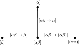
Figure 1. Arboreal singularity $\overline{\mathbb{A}_{2}}$. For simplicity we use the notation described above for each correspondence.

Example.

We write $A_{3}$ for the tree $\bullet-\bullet-\bullet$, whose vertices we label $\alpha-\beta-\gamma$. There are eleven correspondences: the trivial one, four correspondences of the form $[\bullet\to\bullet]\twoheadleftarrow\dots$ and six of the form $[\bullet]\twoheadleftarrow\dots$. There are 45 strata in the order complex $\overline{\mathbb{A}_{3}}$: 11 zero-dimensional, 22 one-dimensional and 12 two-dimensional strata, assembled as in Figure 2. The link $\mathbb{A}_{3}^{link}$ can be glued out of copies of $\overline{\mathbb{A}_{2}}$.

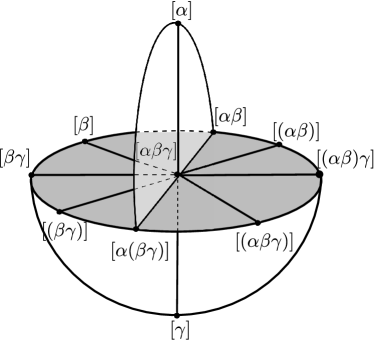
Figure 2. Arboreal singularity $\overline{\mathbb{A}_{3}}$. This singularity is homeomorphic to a union of three 2-discs, along half-discs; in the figure above the grey disc is horizontal and the two white half-discs discs are glued to it along two perpendicular diametersk, one to the top and another to the bottom. We only labelled the 0-simplices; the labels on all other simplices can be deduced from their vertices. The link $\mathbb{A}_{3}^{\mathrm{{link}}}$ can be seen to be homeomorphic to the 1-skeleton of a tetrahedron.

4.1.3. Tree quiver representations

We recall some standard facts about representations of tree quivers. These facts can be found in many sources, e.g. [42, 77]. Let $\vv T$ be a finite quiver, i.e., a finite directed graph. We write $k[\vv T]$ for the path algebra of the quiver, whose generators are the vertices and arrows, subject to the relations that the vertex generators are idempotent, and $fg=0$ unless the head of $f$ is the tail of $g$ (and the head and tail of a vertex are itself). That is, we read paths from left to right. Quiver representations correspond to right modules over this algebra; we write $\operatorname{mod}(\vv T)$ for the (underived!) abelian category of such modules, $\operatorname{Mod}(\vv T)$ for the dg modules, and $\operatorname{Perf}(\vv T)$ for the perfect dg modules. Note $\operatorname{Mod}(\vv T)\in\operatorname{DGCat}$, $\operatorname{Perf}(\vv T)\in\operatorname{dgcat}$, and indeed $\operatorname{Mod}(\vv T)=\operatorname{Ind}\operatorname{Perf}(\vv T)$.

Henceforth we restrict attention to the case when the underlying graph of $\vv T$ is a tree. In this case the path algebra $k[\vv T]$ is smooth and proper, so the perfect and pseudoperfect modules coincide.

For vertices $\alpha,\beta\in\vv{T}$, we write $\alpha\geq\beta$ when there is a path from $\alpha$ to $\beta$, and we denote this unique path by $|\alpha\rangle\langle\beta|$. These compose in the usual way, $|\alpha\rangle\langle\beta||\beta\rangle\langle\gamma|=|\alpha\rangle\langle\gamma|$, and all other compositions vanish. We are particularly interested in the case when the edge directions arise from the choice of a fixed root vertex of $T$, by directing all the edges toward the root. We pronounce $\alpha\geq\beta$ as “alpha is above beta” or “beta is below alpha”, so that everything is above the root. For any vertex $\alpha$, we denote $\hat{\alpha}$ to be the unique vertex such that there is an arrow of length one from $\alpha\to\hat{\alpha}$, i.e., the unique vertex directly below $\alpha$.

We write $P_{\alpha}:=|\alpha\rangle\langle\alpha|k[\vv T]$ for the right module of “paths from $\alpha$”. All paths must have a beginning, and so:

Lemma 4.6.

There is an isomorphism of right $\vv T$ modules $k[\vv T]=\bigoplus_{\alpha}P_{\alpha}$, and $\operatorname{Hom}_{\operatorname{mod}(\vv T)}(P_{\alpha},P_{\beta})$ vanishes unless $\alpha\leq\beta$, in which case it is one dimensional, generated by composition on the left with the unique path $|\beta\rangle\langle\alpha|$.

In particular, the $P_{\alpha}$ are the indecomposable projectives of $\operatorname{mod}(\vv T)$, and in particular their Homs are calculated by the same formula in $\operatorname{Mod}(\vv T)$.

Example.

For the quiver $1\to 2\to 3\to\cdots\to n$, the path algebra can be identified with an algebra of triangular $n\times n$ matrices. The matrix $|i\rangle\langle j|$ corresponds to the unique path from the $i$th vertex to the $j$th vertex. The composition $|i\rangle\langle j||j\rangle\langle k|=|i\rangle\langle k|$ corresponds to the left-to-right composition rule $(i\to j)(j\to k)=(i\to k)$.

Let us now discuss maps of path algebras induced by correspondences of trees. We write $\operatorname{Alg}_{\mathrm{fdsm}}$ for the (ordinary) category of smooth finite dimensional algebras with morphisms given by algebra morphisms; recall that $k[\vv T]$ is always such an algebra.

Lemma 4.7.

To an inclusion $\vv S\overset{i}{\hookrightarrow}\vv T$ we associate an injective map of algebras $i_{\flat}:k[\vv S]\to k[\vv T]$, covariant with respect to compositions of inclusions, and to a quotient $\vv S\overset{q}{\twoheadrightarrow}\vv R$, we associate another injective map of algebras $q^{\sharp}:k[\vv R]\to k[\vv S]$, contravariant with respect to compositions of surjections.

Proof.

We construct both of these maps explicitly by giving the map on the set of paths, and then checking that they respect composition. Let us start with $i_{\flat}$: consider $|\alpha\rangle\langle\beta|$ a path in $\vv S$. We define the following set of vertices in $\vv T$:

$$\ell(\alpha):=\{\gamma\in V(T)\setminus V(S)\ |\ \gamma>\alpha\text{\ and\ }\hat{\alpha}\in V(S)\}$$

In other words, $\ell(\alpha)$ is the set of vertices that are one edge away from $\vv S$ and above $\alpha$. We then define

$$i_{\flat}(|\alpha\rangle\langle\beta|):=|\alpha\rangle\langle\beta|-\sum_{\gamma\in\ell(\alpha)}|\gamma\rangle\langle\beta|.$$

One can directly check that this map respect path compositions and that it is functorial for compositions of inclusions.

Let us now construct $q$, by first defining a section $s$ of the map induced by $q$ on vertex sets: for a vertex $\alpha$ of $\vv R$, we define $s(\alpha)$ to be the lowest vertex in the preimage $q^{-1}(\alpha)$. The map $q^{\sharp}$ is then define on paths by sending $|\alpha\rangle\langle\beta|$ to $|s(\alpha)\rangle\langle s(\beta)|$. One can readily check that this map behaves well under path composition, and is functorial for compositions of quotients. ∎

We then put together the maps above into a functor from the arboreal category $\operatorname{Arb}$.

Lemma 4.8.

There is a functor $\mathcal{I}:\vv\operatorname{Arb}^{op}\to\operatorname{Alg}_{\mathrm{fdsm}}$ which maps a rooted tree $\vv T$ to the algebra $k[\vv T]$ and the morphism $\vv R\to\vv T$ defined by the correspondence $(R\overset{q}{\twoheadleftarrow}S\overset{i}{\hookrightarrow}T)$ to the map of algebras given by $i_{\flat}\circ q^{\sharp}$.

Proof.

Note we are defining a functor between ordinary (not $\infty$) categories. We check that the compositions of correspondences get mapped to compositions of algebra maps. Consider a composition of correspondences given by the diagram

Functoriality of $\mathcal{I}$ is equivalent to the equality $q^{\sharp}\circ(i^{\prime})_{\flat}=(i^{\prime\prime})_{\flat}\circ(q^{\prime\prime})^{\sharp}$. This can be checked from the definitions of the maps of path algebras, recalling that the pullback $Q\times_{R}S$ can be identified with a subtree of $S$ (therefore also a subtree of $T$) on all the vertices that map to the image of $Q$ in $R$. ∎

Finally we recall that quivers corresponding to the same underlying tree but with different arrow orientations have representation categories related by reflection functors, defined in [5]. A source (sink) is a vertex that only has outgoing (ingoing) arrows. Given a source $\alpha$, let $s_{\alpha}\vv T$ be the quiver obtained by reversing all the arrows at $\alpha$. There is a reflection functor $R^{+}_{\alpha}:\operatorname{mod}(\vv T)\to\operatorname{mod}(s_{\alpha}\vv T)$, which in fact preserves compact objects and so induces a dg derived equivalence $\operatorname{Perf}(\vv T)\to\operatorname{Perf}(s_{\alpha}\vv T)$. Likewise, at sinks there are similar reflection functors $R^{-}_{\alpha}$. The quiver structure for a rooted tree has all arrows pointing to the root. Because the underlying graph is acyclic, two such structures corresponding to different roots $\rho_{1},\rho_{2}$ can be related by a sequence of moves $s_{\alpha}$. Thus the derived categories $\operatorname{Mod}(\vv T)$ and $\operatorname{Perf}(\vv T)$ depends only on the underlying tree (up to non-canonical equivalence). Choosing a root determines a $t$-structure, and thus the distinguished set of projective generators $\{P_{\alpha}\}$.

4.1.4. A representation of Arb in categories of quiver representations

If $f:A\to B$ is a morphism of algebras, then we denote the restriction of scalars

$$f^{*}:\operatorname{Mod}(B) \to \operatorname{Mod}(A)$$

$$N \mapsto N|_{A}.$$

Its left adjoint is the extension of scalars

$$f_{!}:\operatorname{Mod}(A) \to \operatorname{Mod}(B)$$

$$M \mapsto M\otimes_{A}B.$$

These functors can be organized into $\infty$-functors to $\infty$-categories of dg categories. The following is a restatement of description of the functor in [61, Cor.4.8.5.13], for the case where the ambient monoidal category is $\operatorname{Vect}$.

Lemma 4.9.

There is an $\infty$-functor

$$\operatorname{Mod}_{!}:\operatorname{N}(\operatorname{Alg})\to\operatorname{DGCat},$$

which maps an algebra $A$ to the dg category $\operatorname{Mod}(A)$ of right A-modules, and a morphism of algebras $f:A\to B$ to the extension of scalars $f_{!}$.

Evidently restriction of scalars always preserves pseudo-perfectness (i.e., perfectness over $k$). Meanwhile if $f:A\to B$ presents $B$ as a perfect module over $A$, then the extension of scalars restricts to a morphism $f_{!}:\operatorname{Perf}(A)\to\operatorname{Perf}(B)$. In that case, denoting by $\operatorname{Alg}_{\mathrm{perf}}$ the subcategory of $\operatorname{Alg}$ on such maps, the functor of the lemma above restricts to a functor

$$\operatorname{Perf}_{!}:\operatorname{N}(\operatorname{Alg}_{\mathrm{perf}})\to\operatorname{dgcat}$$

In particular, if $A$ and $B$ are both smooth and finite dimensional, $B$ is pseudoperfect over $A$ hence perfect hence $f_{!}$ preserves perfect modules, and since pseudoperfect and perfect modules agree, also $f^{*}$ preserves perfect modules. In this case we have an adjunction $(f_{!},f^{*})$ of functors on perfect modules, and by composing the functor above with taking right adjoints we get another functor

$$\operatorname{Perf}^{*}:\operatorname{N}(\operatorname{Alg}_{\mathrm{fdsm}})\to\operatorname{dgcat}^{op},$$

which maps a morphism of algebras $f:A\to B$ to the pullback $f^{*}$.

By the discussion above, once we restrict $\operatorname{Perf}_{!}$ to finite-dimensional smooth algebras, there is a natural equivalence $(\operatorname{Perf}^{*})^{op}\simeq(-)^{pp}\circ\operatorname{Perf}_{!}$, i.e. the image of $\operatorname{Perf}^{*}$ can be obtained by taking pseudo-perfect modules.

Let us use these functors in the context of correspondences between rooted trees. Recall that the algebras $k[\vv T]$ are always smooth and finite dimensional.

Definition 4.10.

The arboreal functors are given by the compositions

$$\mathcal{A}_{!} :\vv\operatorname{Arb}\xrightarrow{\mathcal{I}}(\operatorname{Alg}_{\mathrm{fdsm}})^{op}\xrightarrow{\operatorname{Perf}_{!}}\operatorname{dgcat}^{op}$$

$$\mathcal{A}^{*} :\vv\operatorname{Arb}\xrightarrow{\mathcal{I}}(\operatorname{Alg}_{\mathrm{fdsm}})^{op}\xrightarrow{\operatorname{Perf}^{*}}\operatorname{dgcat}.$$

In other words, both functors map a rooted tree $\vv T$ to the category $\operatorname{Perf}(k[\vv T])$; and on morphisms, $\mathcal{A}_{!},\mathcal{A}^{*}$ maps a correspondence $\mathfrak{p}=\vv R\overset{q}{\twoheadleftarrow}\vv S\overset{i}{\hookrightarrow}\vv T$ to the functors

$$\mathfrak{p}_{!}=(q^{\sharp}\circ i_{\flat})_{!}:\operatorname{Perf}(k[\vv R])\to\operatorname{Perf}(k[\vv T]),\qquad\mathfrak{p}^{*}=(q^{\sharp}\circ i_{\flat})^{*}:\operatorname{Perf}(k[\vv T])\to\operatorname{Perf}(k[\vv R])$$

respectively.

Let us characterize ${\mathfrak{p}}^{*}$ explicitly.

Lemma 4.11.

Consider a correspondence $\mathfrak{p}:\vv R\overset{q}{\twoheadleftarrow}\vv S\overset{i}{\hookrightarrow}\vv T$, and any vertex $\alpha\in T$. Then there is an equivalence

$${\mathfrak{p}}^{*}(P_{\alpha})\cong\begin{cases}P_{q(i^{-1}(\alpha))}&\qquad\alpha\in i(S)\\ 0&\qquad\text{otherwise.}\end{cases}$$

The morphism $\operatorname{Hom}_{\vv T}(P_{\alpha},P_{\beta})\to\operatorname{Hom}_{\vv R}({\mathfrak{p}}^{*}(P_{\alpha}),{\mathfrak{p}}^{*}(P_{\beta}))$ sends $|\beta\rangle\langle\alpha|\to|q(i^{-1}(\beta))\rangle\langle q(i^{-1}(\alpha))|$ (and hence is an isomorphism) when these are defined; otherwise it is zero.

Proof.

Let us compute the maps induced by $i$ and $q$ separately. We compute $i_{\flat}^{*}(P_{\alpha})$ by studying the action of paths $|\beta\rangle\langle\beta^{\prime}|$ in $\vv S$; right-composition of some path in $P_{\alpha}$ with the image of this under $i_{\flat}$ is then given by calculating the composition

$$|\alpha\rangle\langle\alpha^{\prime}|\cdot\left(|\beta\rangle\langle\beta^{\prime}|-\sum_{\gamma\in\ell(\beta)}|\gamma\rangle\langle\beta^{\prime}|\right)$$

in $k[\vv T]$. There are four cases to analyze: $\alpha<\vv S,\in\vv S,>\vv S$ (where by the inequality we mean there is some vertex in $\vv S$ for which it holds) or $\alpha$ is incomparable with any vertex in $\vv S$; we check that this is zero in the first, third and fourth case, and only nonzero in the second case when $\alpha^{\prime}=\beta$, in which case it is one-dimensional. This identifies the module with $P_{i^{-1}(\alpha)}$.

Let us now compute $(q^{\sharp})^{*}$, by looking instead at the simple modules $S_{\alpha}=P_{\alpha}/P_{\hat{\alpha}}$, supported only on the vertex $\alpha$. The map $S\twoheadrightarrow R$ is given by successive contraction of connected subtrees $Q$; the only nontrivial case to check is when $\alpha\in V(Q)$; then a path $|\beta\rangle\langle\beta^{\prime}|$ in $k[\vv R]$ acts by zero unless $\alpha=\beta=\rho$ where $\rho$ is the root of $Q$; for $\alpha\notin V(Q)$ the path acts by zero unless $\alpha=\beta$. In other words, $(q^{\sharp})^{*}$ sends $S_{\alpha}$ to $S_{q(\alpha)}$ if $\alpha\notin V(Q)$ and kills all simples supported in $Q$ except for the root; it then identifies all the projectives corresponding to vertices in $Q$.

As for the morphisms, the only nontrivial morphism between the $P_{\alpha}$s is given by composition with a unique path; since we calculated the action of arbitrary paths above we can deduce the second part of the statement. ∎

Remark.

Comparing the functor Lemma 4.11 to the description in [68, Sec.4.2] shows that the (co)sheaf we have constructed here agrees with the Nadler’s calculation of the microlocal sheaf categories.

4.2. Sheaves and cosheaves on an arboreal singularity

4.2.1. Constructible sheaves on simplicial complexes

We briefly recall how to describe constructible sheaves on a simplicial complex. For a simplex $\sigma$ in a simplicial complex $X$, we write $\operatorname{Star}(\sigma)$ for the union of open simplices whose closure contains $\sigma$. To give a sheaf $\mathcal{F}$ on $X$, constructible with respect to the stratification by simplices, it suffices to give the values of $\mathcal{F}$ on the open sets $\operatorname{Star}(\sigma)$, and the corresponding restriction maps $\mathcal{F}(\operatorname{Star}(\sigma))\to\mathcal{F}(\operatorname{Star}(\tau))$ when $\operatorname{Star}(\tau)\subset\operatorname{Star}(\sigma)$, i.e., when $\sigma$ lies in the closure of $\tau$. The appropriate diagrams should commute. Our definition of simplicial complex demands that the closure of an open simplex is a closed simplex, so there are no non-trivial overlaps, hence no descent conditions.

The restriction $\mathcal{F}(\operatorname{Star}(\sigma))\to\mathcal{F}_{\sigma}$ is then necessarily an isomorphism, so one can instead discuss ‘generization maps’ $\mathcal{F}_{\sigma}\to\mathcal{F}_{\tau}$ when $\sigma$ lies in the closure of $\tau$; this is the so-called ‘exit path’ description of a constructible sheaf. A similar description works for any sufficiently fine stratification satisfying appropriate local contractibility conditions.

From a functor $F:\mathcal{X}\to\mathcal{Y}$ we may extract the generization maps for a $\mathcal{Y}$-valued constructible sheaf $\operatorname{N}(F)$ on the geometric realization of the nerve $|\operatorname{N}(\mathcal{X})|$, as follows. On objects, we set

$$\operatorname{N}(F)([x_{1}\to x_{2}\to\cdots\to x_{n}])=F(x_{n})$$

and the generization maps are given by

$$\operatorname{N}(F)([x_{m}\to\cdots\to x_{m^{\prime}}]\to[x_{1}\to x_{2}\to\ldots\to x_{n}])=F(x_{m}^{\prime}\to x_{n}),$$

where the map $x_{m}^{\prime}\to x_{n}$ comes from the fact that $x_{m}\to\cdots\to x_{m^{\prime}}$ was a subsequence of $x_{1}\to x_{1}\to\ldots\to x_{n}$. The fact that $F$ was a functor translates to the compatibility of the generization maps.

Note however that in order for this data to define a sheaf valued in $\mathcal{Y}$, we must be able to say what values it takes on unions of strata. These will be given by a limit. In the setting at hand, we will work with finite stratifications, so insist that $\mathcal{Y}$ be closed under finite limits.

Remark.

Though it is not necessary, one can rephrase the above in the language of exit-path categories, as developed in [61, Sec.A.6]. For any $A$-stratified space $X$, one can associate an $\infty$-category $\operatorname{Sing}^{A}(X)$, its exit-path category, such that there is an equivalence

$$\operatorname{Fun}(\operatorname{Sing}^{A}(X),\mathcal{C})\simeq\operatorname{Sh}^{A}(X,\mathcal{C})$$

for any $\infty$-category $\mathcal{C}$ with small limits. In the case where $X=|\operatorname{N}(\mathcal{X})|$ for some category $\mathcal{X}$, with its natural stratification $A$, there is an equivalence $\operatorname{Sing}^{A}(|\operatorname{N}(\mathcal{X})|)\simeq\operatorname{N}(\mathcal{X})$ so any functor out of $\mathcal{X}$ determines a constructible sheaf on the geometric realization of the nerve. If the nerve is finite, then we do not need to require $\mathcal{C}$ to have all small limits; it is enough to require existence of finite limits, which is satisfied e.g. by $\operatorname{dgcat}$.

4.2.2. The arboreal sheaf and cosheaf

Let $T$ be a tree. Recall that we have a category $\operatorname{Arb}_{T}$ and a space $\overline{\mathbb{T}}:=\operatorname{N}(\operatorname{Arb}_{T})$. Choosing a root determines a quiver $\vv T$, giving a category $\vv\operatorname{Arb}_{\vv T}$ which is equivalent to $\operatorname{Arb}_{T}$. Composing the functors of Definition 4.10 with the forgetful functor $\vv\operatorname{Arb}_{\vv T}\to\vv\operatorname{Arb}$, we have functors $\mathcal{A}^{*}:\operatorname{Arb}_{T}\to\operatorname{dgcat}^{op}$ and $\mathcal{A}_{!}:\operatorname{Arb}_{T}\to\operatorname{dgcat}$.

Definition 4.12.

The arboreal sheaf $\mathcal{A}_{\vv T}\in\operatorname{Sh}(\overline{\mathbb{T}},\operatorname{dgcat})$ is the sheaf associated to the functor $\mathcal{A}^{*}$, and the arboreal cosheaf $\mathcal{A}^{co}_{\vv T}\in\operatorname{Cosh}(\overline{\mathbb{T}},\operatorname{dgcat})$ is the cosheaf associated to the functor $\mathcal{A}_{!}$.

Note that by definition of the functors $\mathcal{A}^{*}$ and $\mathcal{A}_{!}$, the arboreal cosheaf and sheaf are both locally saturated; we then have a smooth ccc space $(\overline{\mathbb{T}},\mathcal{A}_{\vv T}^{co})$ and a proper csc space $(\overline{\mathbb{T}},\mathcal{A}_{\vv T})$, with the arboreal singularity as underlying topological space; also we have $\mathcal{A}_{\vv T}=(\mathcal{A}_{\vv T}^{pp})$.

Remark.

Here we understand the topology on $\overline{\mathbb{T}}$ as being the stratification topology: stars of strata are the basis of opens. The relevance of this is that $\operatorname{dgcat}$ has (only) homotopy finite limits and colimits.

Writing this topological space as $\overline{\mathbb{T}}^{str}$ and the usual topology as $\overline{\mathbb{T}}^{us}$, there is a continuous map $t:\overline{\mathbb{T}}^{us}\to\overline{\mathbb{T}}^{str}$. To pull back the sheaf or cosheaf, we would however have to change the target category from $\operatorname{dgcat}$ to $\operatorname{DGCat}$ so as to have all limits and colimits. Having done so we may consider the sheaf or cosheaf $t^{*}\operatorname{Ind}\mathcal{A}_{\vv T}$ in the usual topology.

For brevity we will usually drop the subscript $\vv T$ when it is unambiguous. Let us describe the arboreal sheaf explicitly. Let $\mathfrak{p}$ be a correspondence $R\twoheadleftarrow S\hookrightarrow T$. We write $\mathbb{T}(\mathfrak{p})$ for the union of all simplices $[\mathfrak{p}_{1}\to\mathfrak{p}_{2}\cdots\to\mathfrak{p}]$. Then $\overline{\mathbb{T}}=\coprod\mathbb{T}(\mathfrak{p})$, and, by definition, any sheaf associated to a functor from $\operatorname{Arb}_{T}$ is constant on the $\mathbb{T}(\mathfrak{p})$. In fact, each $\mathbb{T}(\mathfrak{p})$ with $\mathfrak{p}\neq\mathfrak{p}_{T}$ is topologically an open cell of dimension $|T|-|R|$ [68, Prop 2.14]. The cone point $\mathbb{T}(\mathfrak{p}_{T})$ is the unique zero dimensional cell. Moreover, $\overline{\mathbb{T}(\mathfrak{p})}=\coprod_{\mathfrak{p}^{\prime}\leq\mathfrak{p}}\mathbb{T}(\mathfrak{p}^{\prime})$ [68, Prop. 2.18].

Figure 3. Stratification of the arboreal singularity $\overline{\mathbb{A}}_{2}$, by the strata $\mathbb{A}_{2}(\mathfrak{p})$.

Fix $\vv T$ and denote $\mathcal{A}=\mathcal{A}_{\vv T}$. Because $\mathcal{A}$ is constructible with respect to a stratification by a union of cells which all adjoin $\mathfrak{p}_{T}$, the restriction map $\Gamma(\mathbb{T},\mathcal{A})\to\mathcal{A}_{\mathfrak{p}_{T}}$ is an isomorphism. In particular, $\Gamma(\mathbb{T},\mathcal{A})\simeq\operatorname{Perf}(\vv{T})$. Given an object $X\in\Gamma(\mathbb{T},\mathcal{A})=\operatorname{Perf}(\vv{T})$, the germ at a point in $\mathbb{T}(R\twoheadleftarrow S\hookrightarrow T)$ is an element of the category $\operatorname{Perf}(\vv{R})$. The desired object is produced by applying the correspondence functor $c_{\mathfrak{p}}$ obtained from $(R\twoheadleftarrow S\hookrightarrow T)$ to $X$.

4.2.3. Hom sheaves

Recall that given a sheaf of categories $\mathcal{F}$ and objects $x,y\in\mathcal{F}(X)$, there is a sheaf $\mathcal{F}|_{X}^{x,y}\in\operatorname{Sh}(X,\operatorname{Vect})$ which on $U$ evaluates to $\operatorname{Hom}_{\mathcal{F}(U)}(\rho x,\rho y)$. For ease of notation, we will denote

$$\mathcal{A}_{\alpha,\beta}:=\mathcal{A}|_{\mathbb{T}}^{P_{\alpha},P_{\beta}}$$

for the Hom sheaf between the generating projectives.

We will need explicit descriptions of the Hom sheaves between the generating projectives $P_{\alpha}$. Since we know what the functors $c_{\mathfrak{p}}$ do to the projective objects from Lemma 4.11, it is just a matter of assembling the sheaf of the morphisms between Hom spaces.

Definition 4.13.

For $\alpha$ a vertex of $T$, we write

$$\mathbb{T}(\alpha):=\coprod_{\alpha\in S}\mathbb{T}(R\twoheadleftarrow S\hookrightarrow T).$$

Remark.

In [68], Nadler gives an explicit construction of the arboreal singularities: for each vertex $\alpha$ of $T$, take a copy of $\mathbb{R}^{|T|-1}$ with coordinates $x^{\gamma}(\alpha),\gamma\neq\alpha$. The topological space $\mathbb{T}$ is recovered by gluing these spaces: for each edge $\{\alpha,\beta\}\in E(T)$, identify points with coordinates $x_{\gamma}(\alpha)$ and $x_{\gamma}(\beta)$ whenever $x_{\beta}(\alpha)=x_{\alpha}(\beta)\geq 0$ and $x_{\gamma}(\alpha)=x_{\gamma}(\beta)$ for $\gamma\neq\alpha,\beta$. Comparing this construction with the combinatorial definition [68, Sec. 2] it is proven that the strata $\mathbb{T}(R\twoheadleftarrow S\hookrightarrow T)$ sit in the closure of the Euclidean space corresponding to $\alpha$ exactly when $\alpha\in S$. Thus $\mathbb{T}(\alpha)$ is homeomorphic to a closed ball of dimension $|T|-1$.

Figure 4. Gluing of $\overline{\mathbb{A}}_{3}$ from the discs $\mathbb{A}_{3}(\bullet)$. $\mathbb{A}_{3}(\alpha)$ and $\mathbb{A}_{3}(\gamma)$ are shown creased, with half-disc flaps pointing up and down, respectively.

The following calculations are new.

Proposition 4.14.

The sheaf $\mathcal{A}_{\alpha,\alpha}\in\operatorname{Sh}(\mathbb{T},\operatorname{Vect})$ is the constant rank one (in degree zero) sheaf on $\mathbb{T}(\alpha)$.

Proof.

Let us describe the functor on $\operatorname{Arb}_{T}$ whose nerve is the sheaf $\mathcal{A}_{\alpha,\alpha}$. By Lemma 4.11, on objects this functor is:

$$(R\twoheadleftarrow S\hookrightarrow T)\mapsto\operatorname{Hom}_{\vv R}(P_{q(i^{-1}(\alpha))},P_{q(i^{-1}(\alpha))})=\begin{cases}k,\qquad\alpha\in i(S)\\ 0,\qquad\mathrm{otherwise.}\end{cases}$$

These Hom spaces have the identity as a basis element, which must be preserved by the functorial structure, hence gives a global section trivializing the sheaf hom. ∎

To describe other Hom sheaves we have to worry about the orientation of the arrows in the quiver. For any pair of vertices $\alpha,\beta$, consider the following subset of $\mathbb{T}$:

$$\mathbb{T}(\alpha,\beta):=\coprod_{\begin{subarray}{c}\alpha,\beta\in S\\ q(i^{-1}(\alpha))\leq q(i^{-1}(\beta))\end{subarray}}\mathbb{T}(R\twoheadleftarrow S\hookrightarrow T).$$

Figure 5. The subsets $\mathbb{A}_{3}(\bullet,\bullet)$ where $\mathbb{A}_{3}$ has the quiver structure $\alpha\rightarrow\beta\leftarrow\gamma$. The subsets $\mathbb{A}_{3}(\alpha),\mathbb{A}_{3}(\beta),\mathbb{A}_{3}(\gamma)$ are homeomorphic to closed discs, and the arboreal singularity is obtained by gluing them appropriately; on the left $\mathbb{A}_{3}(\alpha),\mathbb{A}_{3}(\gamma)$ are shown with folded flaps up and down, and are glued along the horizontal parts to $\mathbb{A}_{3}(\beta)$. Note that the subsets $\mathbb{T}(\lambda_{1},\lambda_{2})$ depend on the directions of the arrows in $T$, and moreover as in the proof above for any vertices $\lambda_{1},\lambda_{2}$, the difference between $\mathbb{T}(\lambda_{1},\lambda_{2})$ and $\mathbb{T}(\lambda_{1})\cap\mathbb{T}(\lambda_{2})$ is at most deletion of some boundary strata.

Proposition 4.15.

The sheaf $\mathcal{A}_{\alpha,\beta}$ is the constant rank one sheaf on $\mathbb{T}(\alpha,\beta)$.

Proof.

Again, let us write the functor on $\operatorname{Arb}$ giving rise to this sheaf. By Lemma 4.11, on objects it is

$$(R\twoheadleftarrow S\hookrightarrow T)\mapsto\operatorname{Hom}_{\vv R}(P_{q(i^{-1}(\alpha))},P_{q(i^{-1}(\beta))})=\begin{cases}k,\qquad\alpha,\beta\in S\,\,\&\,\,q(\alpha)\leq q(\beta)\\ 0,\qquad\mathrm{otherwise.}\end{cases}$$

Here, when $\alpha\notin S$, we interpret $P_{q(i^{-1}(\alpha))}$ as $0$; and similarly for $\beta$. This shows that the sheaf has the correct stalks. Lemma 4.11 also described how the functor acts on the natural basis for these spaces, showing that the sheaf is locally constant and in fact giving a global section, showing it is constant.

Another way to see that to see the sheaf is constant is to explicitly describe the locus $\mathbb{T}(\alpha,\beta)$ and show it is contractible. First, note that $\mathbb{T}(\alpha,\beta)\subseteq\mathbb{T}(\alpha)\cap\mathbb{T}(\beta)$, with equality if $\alpha\leq\beta$. Since $\mathbb{T}(\alpha)$ and $\mathbb{T}(\beta)$ are both homeomorphic to $\mathbb{R}^{|T|-1}$ and are glued together along a half-space, their intersection is homeomorphic to a closed ball. For the case where $\alpha\nleq\beta$, the inclusion is strict, so suppose that we have a simplex

$$[\mathfrak{p}_{1}\to\dots\to\mathfrak{p}_{m}]\subset(\mathbb{T}(\alpha)\cap\mathbb{T}(\beta))-\mathbb{T}(\alpha,\beta).$$

If we denote $\mathfrak{p}_{m}=(R_{m}\twoheadleftarrow S_{m}\hookrightarrow T)$, this is the same as having $\alpha,\beta\in S_{m}$ but $q(\alpha)\neq q(\alpha\vee\beta)$. Consider now the correspondence $\mathfrak{q}=(R\twoheadleftarrow Q\hookrightarrow R_{m})$, where $Q$ is some subtree of $R_{m}$ containing $q(\alpha)$ but not containing $q(\beta)$. Then $\beta\notin Q\times_{R_{m}}S_{m}$, which means the simplex $[\mathfrak{p}_{1}\to\dots\mathfrak{p}_{m}\to\mathfrak{p}_{m}\to\mathfrak{q}\circ\mathfrak{p}_{m}]$ is in $\mathbb{T}(\alpha)$ but not in $\mathbb{T}(\beta)$, so this simplex is contained in the boundary of $\mathbb{T}(\alpha)\cap\mathbb{T}(\beta)$. Thus $\Lambda(\alpha,\beta)$ is obtained by deleting parts of the boundary of the closed ball $\mathbb{T}(\alpha)\cap\mathbb{T}(\beta)$,so it is contractible. ∎

4.2.4. Generalized arboreal singularities

In the expansion of Legendrian singularities, certain additional ‘generalized arboreal singularities’ appear [69]. Such a space is obtained from an ordinary arboreal singularity by deleting some of the strata; its data is encoded by a rooted tree $\vv T$ together with a subset of marked leaves $\ell\subseteq V(T)$, such that every element of $\ell$ is maximal for the partial order induced by the rooting. Let us define $\vv T^{+}$ to be the rooted tree obtained from $\vv T$ by adjoining a new vertex $\alpha^{+}$ for each $\alpha\in\ell$, with a new edge $\alpha^{+}\to\alpha$.

Definition 4.16.

(following Prop. 4.29 in [69]) The generalized arboreal singularity $\overline{\mathbb{T}}^{*}$ corresponding to $(\vv T,\ell)$ is the stratified space obtained from the arboreal singularity $\overline{\mathbb{T}}^{+}$ by deleting the union $Y$ of subsets $\mathbb{T}^{+}(\mathfrak{p}_{\alpha})\cup\mathbb{T}^{+}(\mathfrak{p}_{(\alpha^{+}\alpha)})$ for every $\alpha\in\ell$. We denote $\mathbb{T}^{*}=\mathbb{T}^{+}\cap\overline{\mathbb{T}}^{*}$.

From the construction of Section 3.3, there is a locally saturated cosheaf on $\mathbb{T}^{*}$ given by

$$\mathcal{A}^{co}_{\vv T,\ell}:=(\mathcal{A}^{co}_{\vv T})_{\mathbb{T}^{+}/Y}|_{\mathbb{T}^{*}}$$

giving $\mathbb{T}^{*}$ the structure of a ccc space; and also of a csc space with the sheaf $\mathcal{A}_{\vv T,\ell}$ of pseudo-perfect modules.

Figure 6. The generalized arboreal singularity corresponding to the singleton quiver $\vec{T}=\alpha$ with the vertex also a marked leaf $\ell=\{\alpha\}$. We delete two open subsets to get $\overline{\mathbb{T}}^{*}$; also shown is $\mathbb{T}^{*}=\overline{\mathbb{T}}^{*}\cap\mathbb{T}^{+}$.

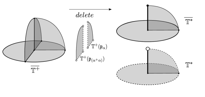
Figure 7. The generalized arboreal singularity corresponding to the $A_{2}$ quiver $\vec{T}=\alpha\to\beta$ with marked leaf $\ell=\{\alpha\}$. Here we obtain $\overline{\mathbb{T}}^{*}$ from deleting some of the strata in the arboreal singularity $\overline{\mathbb{T}}^{+}$ corresponding to the augmented quiver $\alpha^{+}\to\alpha\to\beta$. Bottom right corner shows $\mathbb{T}^{*}$; note that it contains part of its boundary.

5. Orientations on arboreal spaces

5.1. Arboreal spaces

Definition 5.1.

A ccc space $(\mathbb{X},\mathcal{W})$ is special arboreal if it is locally modelled on $(\mathbb{T},\mathcal{A}^{co}_{\vv T})$ for varying $\vv T$.

More precisely, for every $x\in\mathbb{X}$, there is some $\vv T=\vv T(x)$, some refinements of stratifications on $\mathbb{X}$ and $\mathbb{T}$, after which there is some stratified neighborhood $\mathbb{U}\ni x$ and a stratified embedding $m:\mathbb{U}\hookrightarrow\mathbb{T}$ and an isomorphism $\mathcal{W}|_{\mathbb{U}}\cong m^{*}\mathcal{A}^{co}_{\vv T}|_{\mathbb{U}}$.

Note that we ask $\mathbb{X}$ is locally modelled on the interiors $\mathbb{T}$ of the arboreal singularities $\overline{\mathbb{T}}$.

Remark.

Because the spaces $(\mathbb{T},\mathcal{A}_{\vv T})$ are themselves, away from the central point, locally modelled on other such spaces for smaller trees, in the above definition we could equivalently ask that $x$ maps to the central point of $\mathbb{T}$ if we allow $m$ to be a stratified submersion. This would have the virtue of making $T(x)$ a well defined function of $x$.

More generally,

Definition 5.2.

A ccc space $(\mathbb{X},\mathcal{W})$ is arboreal if it is locally modelled on the $(\mathbb{T}^{*},\mathcal{A}^{co}_{\vv T,\ell})$ of Def. 4.16, for varying choices of $(\vv T,\ell)$.

Note that a special arboreal space is an arboreal space in which we choose the set of marked leaves to be empty.

Lemma 5.3.

An arboreal space $(\mathbb{X},\mathcal{W})$ is smooth (i.e. $\mathcal{W}(U)$ is smooth for all $U$) and stalkwise proper. The dual csc space $(\mathbb{X},\mathcal{W}^{pp})$ is proper and stalkwise smooth.

Proof.

Follows from the fact that the cosheaves $\mathcal{A}^{co}_{\vv T,\ell}$ are locally saturated, together with the fact that finite colimits of smooth categories are smooth (see Lemma 8.21). ∎

5.2. An orientation on an arboreal space

Consider an arboreal space $(\mathbb{X},\mathcal{W})$ as above. By Theorem 1.12, which will be proved later in Section 9.3.2, orientations on the ccc space $(\mathbb{X},\mathcal{W})$ are equivalent to orientations on the csc space $(\mathbb{X},\mathcal{W}^{pp})$. Moreover, by Lemma 3.10, we only have to consider orientations on special arboreal spaces.

We will first show the local models $(\mathbb{T},\mathcal{A})$ admit orientations. More precisely, we will show that a rooting of $T$ induces a canonical isomorphism $\mathcal{H}\mathcal{H}(\mathcal{A})\simeq\omega_{\mathbb{T}}[1-|T|]$, which moreover gives an orientation on the csc space $(\mathbb{T},\mathcal{A})$.

5.2.1. The dualizing complex of an arboreal singularity

Verdier’s dualizing complex on a space $X$ is usually defined as $\omega_{X}=pt^{!}k$, where $pt$ is the map to a point. As mentioned in [41, p. 91], an explicit representative is given by the “sheaf of local singular chains”. That is, let ${C}^{-d}$ be the sheaf which on sufficiently small open sets is given by $\mathbf{C}^{-d}(U)=C_{d}(X,X\setminus U;k)$, where $C_{d}$ is the singular $d$-chains, and the sheaf structure is defined by the evident restriction maps. The singular chain differential collects these into a complex of sheaves, which is quasi-isomorphic to the dualizing complex.

Proposition 5.4.

With notation as above, the stalk of $\omega_{\mathbb{T}}$ at a stratum labelled by a correspondence $\mathfrak{p}=(R\twoheadleftarrow S\hookrightarrow T)$ is concentrated in degree $-(n-1)$, where it is given by a direct sum decomposition

$$\omega_{\mathbb{T}}^{-(n-1)}(\mathbb{T}(\mathfrak{p}))\simeq\bigoplus_{\alpha\in R}k_{\alpha}\simeq k^{|R|},$$

where each $k_{\alpha}\simeq k$. Now suppose we have correspondences $\mathfrak{p}^{\prime}=\mathfrak{q}\circ\mathfrak{p}$, where $\mathfrak{p}=(R^{\prime}\twoheadleftarrow S^{\prime}\hookrightarrow T)$ and $\mathfrak{q}=(R^{\prime}\overset{q}{\twoheadleftarrow}Q\overset{i}{\hookrightarrow}R)$. Then the simplex $[\mathfrak{p}]$ is in the closure of $[\mathfrak{p}\to\mathfrak{p}^{\prime}]$ and the generization map $\omega_{\mathbb{T}}(\mathbb{T}(\mathfrak{p}))\to\omega_{\mathbb{T}}(\mathfrak{p}^{\prime})$ is given, in the decomposition above, by

$$\bigoplus_{\alpha\in R}k_{\alpha}\to\bigoplus_{\beta\in R^{\prime}}k_{\beta},$$

where $1\in k_{\alpha}$ gets sent to $1\in k_{q(\alpha)}$ if $\alpha\in S$ and $0$ otherwise. In other words, the map adds all the factors corresponding to vertices that get identified by the quotient $q$. Moreover, if one picks an orientation of a top stratum of $\mathbb{T}$, there is a canonical choice of isomorphisms above.

Proof.

As mentioned above, on any space $X$, for sufficiently small $U$, there is a natural isomorphism $\omega_{X}(U)=C_{*}(X,X\setminus U)$, with the chain complex $C_{*}$ interpreted as a cochain complex just by negating all the degrees.

Let us first calculate the stalk at the center of $\mathbb{T}$, that is at the simplex $[\mathfrak{p}_{0}]$ given by the trivial correspondence. Consider the decomposition of $\mathbb{T}$ into the discs $\mathbb{T}(\alpha)$, and for each vertex $\alpha$ let $U_{\alpha}=U\cap\mathbb{T}(\alpha)$ and $Z_{\alpha}=\mathbb{T}(\alpha)\setminus U_{\alpha}$ where $U$ is a small neighborhood of $[\mathfrak{p}_{0}]$. Each $U_{\alpha}$ is an open disc inside of the disc $\mathbb{T}(\alpha)$, so the relative homology $H_{*}(\mathbb{T}(\alpha),Z_{\alpha})$ is $k$ in degree $n-1$ and zero in other degrees.

For an edge $\alpha-\beta$, the Mayer-Vietoris sequence for relative homology gives a distinguished triangle

$$C_{*}(\mathbb{T}(\alpha)\cap\mathbb{T}(\beta),Z_{\alpha}\cap Z_{\beta})\to C_{*}(\mathbb{T}(\alpha),Z_{\alpha})\oplus C_{*}(\mathbb{T}(\beta),Z_{\beta})\to C_{*}(\mathbb{T}(\alpha)\cup\mathbb{T}(\beta),Z_{\alpha}\cup Z_{\beta})$$

Note that since the discs $\mathbb{T}(\alpha),\mathbb{T}(\beta)$ are glued by their halves, the pair $(\mathbb{T}(\alpha)\cap\mathbb{T}(\beta),Z_{\alpha}\cap Z_{\beta})$ has zero relative homology

$$C_{*}(\mathbb{T}(\alpha)\cap\mathbb{T}(\beta),Z_{\alpha}\cap Z_{\beta})\simeq C_{*}(\text{half-ball},\text{half-sphere})\simeq 0$$

so we can identify

$$C_{*}(\mathbb{T}(\alpha)\cup\mathbb{T}(\beta),Z_{\alpha}\cup Z_{\beta})\simeq C_{*}(\mathbb{T}(\alpha),Z_{\alpha})\oplus C_{*}(\mathbb{T}(\beta),Z_{\beta})\simeq k^{2}[n-1].$$

We can iterate and glue the pairs $\mathbb{T}(\alpha),\mathbb{T}(\beta)$ according to the tree $T$. More specifically, take connected subtrees $Q\subset Q^{\prime}\subseteq T$ such that $|Q^{\prime}|=|Q|+1$, that is the subtree $Q^{\prime}$ is obtained from $Q$ by adding a new vertex $\gamma$ of $T$ with an edge $\beta-\gamma$ for some $\beta\in Q$. Now suppose by induction that we know a direct sum decomposition of the relative cohomology of the pair obtained by taking all $\mathbb{T}(\alpha)$ and $Z_{\alpha}$ with $\alpha\in Q$:

$$C_{*}(\bigcup_{\alpha\in Q}\mathbb{T}(\alpha),\bigcup_{\alpha\in Q}Z_{\alpha})\simeq\bigoplus_{\alpha\in Q}C_{*}(\mathbb{T}(\alpha),Z_{\alpha})\simeq k^{|Q|}[n-1].$$

Note that since we glued $\gamma$ only to one vertex $\beta$ in $Q$, the intersection $(\cup_{\alpha\in Q}\mathbb{T}(\alpha))\cap\mathbb{T}(\gamma)$ coincides with $\mathbb{T}(\beta)\cap\mathbb{T}(\gamma)$, and also $(\cup_{\alpha\in Q}Z_{\alpha})\cap Z_{\gamma}=Z_{\beta}\cap Z_{\gamma}$. So as noted above this pair has vanishing cohomology, and the Mayer Vietoris distinguished triangle

$$C_{*}((\bigcup_{\alpha\in Q}\mathbb{T}(\alpha))\cap\mathbb{T}(\gamma),(\bigcup_{\alpha\in Q}Z_{\alpha})\cap Z_{\gamma})\to C_{*}(\bigcup_{\alpha\in Q}\mathbb{T}(\alpha),\bigcup_{\alpha\in Q}Z_{\alpha})\oplus C_{*}(\mathbb{T}(\gamma),Z_{\gamma})\to C_{*}(\bigcup_{\alpha\in Q^{\prime}}\mathbb{T}(\alpha),\bigcup_{\alpha\in Q^{\prime}}Z_{\alpha})$$

gives us a direct sum decomposition $C_{*}(\bigcup_{\alpha\in Q^{\prime}}\mathbb{T}(\alpha),\bigcup_{\alpha\in Q^{\prime}}Z_{\alpha})\simeq k^{|Q^{\prime}|}[n-1]$ Iterating this until we reach all of $T$ gives the desired result.

Figure 8. The pairs $(\mathbb{T}(\alpha),Z_{\alpha})$ appearing in the Mayer-Vietoris decomposition. The complements $Z_{\alpha}=\mathbb{T}(\alpha)\setminus U_{\alpha}$ are in dark gray. The intersection pairs $(\mathbb{T}(\alpha)\cap\mathbb{T}(\beta),Z_{\alpha}\cap Z_{\beta})$ have vanishing relative homology.

To describe all the other stalks and generization maps, let’s first describe the map

$$(\omega_{\mathbb{T}})_{[\mathfrak{p}_{0}]}\to(\omega_{\mathbb{T}})_{[\mathfrak{p}_{0}\to\mathfrak{p}]}$$

from the central stalk calculated above to the stalk over a neighboring 1-simplex $[\mathfrak{p}_{0}\to\mathfrak{p}]$ where

$$\mathfrak{p}=(R\overset{q}{\twoheadleftarrow}S\hookrightarrow T),$$

with $q$ the contraction of a single edge $\mu-\lambda$. As above, let $U$ be a neighborhood of the origin, and take a point in the simplex $[\mathfrak{p}_{0}\to\mathfrak{p}]$ inside of $U_{0}$. Taking a neighborhood $V\subset U_{0}$ of this point, we see that the map between the two stalks of $\omega_{\mathbb{T}}$ is given by restriction of relative chains.

We use the same decomposition of $\mathbb{T}$ into discs that we have above. Let $V_{\alpha}=V\cap\mathbb{T}(\alpha)$ and $Y_{\alpha}=\mathbb{T}(\alpha)\setminus V_{\alpha}$. We see that $V_{\alpha}=\varnothing$ if $\alpha\notin S$, and if $\alpha\in S$ then the pair $(\mathbb{T}(\alpha),V_{\alpha})$ can be homotoped to $(\mathbb{T}(\alpha),U_{\alpha})$. Moreover, if we consider an edge that’s not being contracted, say $\alpha-\beta\neq\mu-\lambda$, $V_{\alpha}$ and $V_{\beta}$ intersect in an open half-ball inside the closed half-ball $\mathbb{T}(\alpha)\cap\mathbb{T}(\beta)$, so the pair $(\mathbb{T}(\alpha)\cap\mathbb{T}(\beta),Y_{\alpha}\cap Y_{\beta})$ is homotopic to $(\mathbb{T}(\alpha)\cap\mathbb{T}(\beta),Z_{\alpha}\cap Z_{\beta})$ and has vanishing relative homology.

A new feature only occurs for the edge $\mu-\lambda$ being contracted: every stratum adjoining the 1-simplex $[\mathfrak{p}\to\mathfrak{p}_{0}]$ must be labelled by correspondences where this edge is also contracted. So the neighborhood $V$ is entirely contained in the intersection $\mathbb{T}(\mu)\cap\mathbb{T}(\lambda)$, and so the pair $(\mathbb{T}(\mu)\cap\mathbb{T}(\lambda),Y_{\mu}\cap Y_{\lambda})$ is homotopic to $(\mathbb{T}(\mu),Y_{\mu})$ and has relative homology $H_{*}(\mathbb{T}(\mu)\cap\mathbb{T}(\lambda),Y_{\mu}\cap Y_{\lambda})\simeq k[n-1]$.

Now we can apply the same process as above and iterate over all edges of the original tree $T$. Suppose we start with a subtree $Q$ of $T$ such that $Q\subset R,Q\subset S$, meaning no edge of $Q$ gets contracted by $q$, and suppose by induction that we already know a direct sum decomposition

$$C_{*}(\bigcup_{Q}\mathbb{T}(\alpha),\bigcup_{Q}Y_{\alpha})\simeq\bigoplus_{Q}C_{*}(\mathbb{T}(\alpha),Y_{\alpha})\simeq k^{|Q|}[n-1].$$

Consider the Mayer-Vietoris triangle for adjoining an extra vertex $\gamma$ via an edge $\beta-\gamma$ as above. The relative chain restriction maps give a map between the distinguished triangles

Since this is a map of distinguished triangles it suffices to know two of the vertical maps. There are three cases to be checked. Suppose $\gamma\in S$ but $\beta-\gamma\neq\mu-\lambda$: the two terms on the left vanish, and the remaining maps are all isomorphisms. Now suppose $\gamma\notin S$: the two terms on the left vanish, but then since $V_{\gamma}=\varnothing$ the vertical map $C_{*}(\mathbb{T}(\gamma),Z_{\gamma})\to C_{*}(\mathbb{T}(\gamma),Y_{\gamma})$ is zero so the direct sum factor $C_{*}(\mathbb{T}(\gamma),Z_{\gamma})$ of $C_{*}(\cup_{Q^{\prime}}\mathbb{T}(\alpha),\cup_{Q^{\prime}}Z_{\alpha})$ gets killed by the restriction map. The last case to consider is when the vertex being added is $\lambda$ via the contracted edge $\mu-\lambda$. Then the intersection $(\mathbb{T}(\mu)\cap\mathbb{T}(\lambda),Y_{\mu}\cap Y_{\lambda})$ has relative homology $k$ in degree $n-1$ so the map above in degree $n-1$ becomes

Here the middle vertical map $C_{n-1}(\mathbb{T}(\lambda),Z_{\lambda})\to C_{n-1}(\mathbb{T}(\lambda),Y_{\lambda})$ is restriction of relative chains, so it is an isomorphism $k\overset{\sim}{\to}k$. Thus $C_{n-1}(\bigcup_{Q^{\prime}}\mathbb{T}(\alpha),\bigcup_{Q^{\prime}}Y_{\alpha})\simeq k^{|Q|}$, and does not gain an extra direct sum factor $k$ from $C_{n-1}(\mathbb{T}(\lambda),Y_{\lambda})$. A better way of phrasing this is that we have a decomposition

$$C_{*}(\bigcup_{Q^{\prime}}\mathbb{T}(\alpha),\bigcup_{Q^{\prime}}Y_{\alpha})\simeq\bigoplus_{\alpha\in q(Q^{\prime})}k_{\alpha},$$

with one factor $k_{\alpha}\simeq k$ for each vertex $\alpha$ in the image $q(Q^{\prime})\subset R$, since $\mu$ and $\lambda$ contribute only one factor $k_{(\mu\lambda)}$ of $k$. Using this decomposition, we can write down the vertical restriction map on the right as:

$$\bigoplus_{\alpha\in Q^{\prime}}k_{\alpha}\to\bigoplus_{\alpha\in q(Q^{\prime})}k_{\alpha},$$

which is an isomorphism on all factors except for $k_{\mu}\oplus k_{\lambda}\to k_{\mu\lambda}$ where it is addition of cochains.

We can calculate all the other stalks and maps by iterating this procedure, since every correspondence of trees can be decomposed into successive contraction of a single edge; this gives the calculation in the theorem. Note that in order to describe the maps as addition, we implicitly used the fact that we have a distinguished basis element $1\in H_{n-1}(\mathbb{T}(\alpha),Z_{\alpha})$. Picking this element uniquely requires picking a orientation of each disc $\mathbb{T}(\alpha)$; in fact since all discs are glued it is only necessary to pick an orientation of one of the discs, or equivalently an orientation of a top-dimensional stratum of $\mathbb{T}$. ∎

5.2.2. The Hochschild homology and the cyclic homology sheaf

Recall that the Hochschild homology of an algebra $A$ is calculated by the Hochschild chain complex

$$\mathrm{HH}(A):\dots\to A\otimes A\otimes A\to A\otimes A\to A,$$

where $A^{\otimes n}$ is placed in degree $-n$, and the differential $d_{-n}:C_{-n}(A)\to C_{-n+1}(A)$ given by

$$d(x_{n}\otimes\dots\otimes x_{0})=x_{n-1}\otimes\dots\otimes x_{0}x_{n}+\sum_{i=0}^{n-1}(-1)^{i}x_{n}\otimes\dots\otimes x_{i+1}x_{i}\otimes\dots\otimes x_{0}.$$

We are interested in the stalks of the Hochschild homology sheaf $\mathcal{H}\mathcal{H}(\mathcal{A})$ and of the cyclic homology sheaf $\mathcal{H}\mathcal{H}(\mathcal{A})_{S^{1}}$, which are the Hochschild/cyclic homology of the stalks of $\mathcal{A}$, i.e., of the categories $\operatorname{Perf}(\vv T)$. To calculate these, recall that Hochschild/cyclic homology is invariant under dg Morita equivalences, and for any dg-algebra $\mathcal{A}$, there is a quasi-isomorphism of Hochschild complexes $\mathrm{HH}(\mathcal{A})\simeq\mathrm{HH}(\operatorname{Perf}\mathchar 45\relax\mathcal{A})$ with the Hochschild homology of the category of perfect $\mathcal{A}$-modules [49], with compatible $S^{1}$-actions. We recall:

Proposition 5.5.

[15] Let $\vv Q$ be an acyclic quiver. Then $\mathrm{HH}_{0}(k[\vv Q])=k^{|Q|}$ and all higher Hochschild homologies vanish. Moreover the $S^{1}$-action on the Hochschild complex is trivial, i.e. the cyclic complex is given by

$$\mathrm{HH}(k[\vv Q])_{S^{1}}=H^{*}(BS^{1})\otimes\mathrm{HH}(k[\vv Q])=k[u]\otimes\mathrm{HH}(k[\vv Q]),$$

with $u$ denoting canonical generator of $H^{*}(BS^{1})$ in degree $2$, such that the natural map $\mathrm{HH}(k[\vv Q])\to\mathrm{HH}(k[\vv Q])_{S^{1}}$ sends $x\mapsto 1\otimes x$.

Proof.

For convenience of the reader, we indicate the proof. Since $\vv Q$ is a tree, $k[\vv Q]$ has a basis whose elements are the paths from vertex $\alpha$ to vertex $\beta$. These include the idempotents $|\alpha\rangle\langle\alpha|$. Consider the subspace $\Delta_{n}$ of $k[\vv Q]^{\otimes n}$ spanned by the powers of the idempotents $|\alpha\rangle\langle\alpha|^{\otimes n}$, and its complement $L_{n}$ spanned by all other tensor products of paths.

The Hochschild chain complex then splits as $C_{*}(k[\vv Q])=\Delta_{*}\oplus L_{*}$. The complex $L_{*}$ is acyclic, ultimately because $\vv Q$ has no cycles. The diagonal subcomplex $\Delta_{*}$ is $|Q|$ copies of the Hochschild chain complex for the base field $k$.

As for the cyclic homology, consider Connes’ long exact sequence connecting the Hochschild homology $\mathrm{HH}_{*}(k[\vv T])=H^{*}(\mathrm{HH}(k[\vv T]))$ and cyclic homology $\operatorname{HC}_{*}(k[\vv T])=H^{*}(\mathrm{HH}(k[\vv T])_{S^{1}})$:

$$\cdots\to\mathrm{HH}_{n}(k[\vv T])\to\operatorname{HC}_{n}(k[\vv T])\to\operatorname{HC}_{n-2}(k[\vv T])\to\mathrm{HH}_{n-1}(k[\vv T])\to\cdots$$

The result then follows immediately. ∎

Since all the $S^{1}$ actions we consider will be trivial, we will ignore it from now on; every map out of $\mathrm{HH}(k[\vv T])$ can be factored through the map $\mathrm{HH}(k[\vv T])\to\mathrm{HH}(k[\vv T])_{S^{1}}$ by sending $u\mapsto 0$, so for all our applications we can just construct maps out of/into the Hochschild homology $\mathrm{HH}$ itself.

There is a natural basis on $\mathrm{HH}_{0}(\operatorname{Perf}(\vv Q))=\mathrm{HH}_{0}(k[\vv Q])\simeq k^{|Q|}$, given by the images of the idempotents $|\alpha\rangle\langle\alpha|\in k[\vv Q]$, or equivalently, of the modules $P_{\alpha}\in\operatorname{Perf}(\vv Q)$. Note that this basis depends on $\vv{Q}$ and not just the underlying graph. In terms of these bases, Lemma 4.11 gives the generization functors of the Hochschild homology sheaf.

Proposition 5.6.

Let $\mathfrak{p}=(R\twoheadleftarrow S\hookrightarrow T)$ be a correspondence inducing a functor $\operatorname{Perf}(\vv T)\to\operatorname{Perf}(\vv R)$. The induced map between Hochschild homologies is given by

$$|\alpha\rangle\langle\alpha|\mapsto\begin{cases}|q(i^{-1}(\alpha))\rangle\langle q(i^{-1}(\alpha))|&\text{\ if\ }\alpha\in i(S)\\ 0&\text{\ otherwise.}\end{cases}$$

5.2.3. Comparison

Comparing Proposition 5.4 with Propositions 5.5 and 5.6 gives an abstract isomorphism $\mathcal{H}\mathcal{H}(\mathcal{A})\simeq\omega_{\mathbb{T}}[1-n]$.

The choice of this isomorphism is not unique, but as we saw above, upon fixing the decomposition of $\mathbb{T}$ as the union of discs $\mathbb{T}(\alpha)$ and an orientation of one of these discs, we get distinguished bases for the stalks of $\omega_{\mathbb{T}}[1-n]$. In addition if we pick a root in $T$ this induces choices of roots in all $R$, and we get sets of distinguished elements $|\alpha\rangle\langle\alpha|$ in all the stalks of $\mathcal{H}\mathcal{H}(\mathcal{A})$. We can then make a canonical choice of isomorphism $\mathcal{H}\mathcal{H}(\mathcal{A})\xrightarrow{\sim}\omega_{\mathbb{T}}[1-n]$, which on a stalk over the stratum $\mathbb{T}(R\twoheadleftarrow S\hookrightarrow T)$ gives the isomorphism

$$\mathrm{HH}_{0}(k[\vv R])\xrightarrow{\sim}\bigoplus_{\alpha\in V(R)}k_{\alpha},$$

sending $|\alpha\rangle\langle\alpha|$ to $1\in k_{\alpha}\simeq k$ in the direct sum decomposition of proposition 5.4.

Recall we have constructed an isomorphism $\mathcal{H}\mathcal{H}(\mathcal{A})\xrightarrow{\sim}\omega_{\mathbb{T}}[-d]$, with $d=|T|-1$; moreover since the $S^{1}$ action on $\mathcal{H}\mathcal{H}(\mathcal{A})$ is trivial, this naturally descends to an isomorphism $\mathcal{H}\mathcal{H}(\mathcal{A})_{S^{1}}\xrightarrow{\sim}\omega_{\mathbb{T}}[-d]$

Theorem 5.7.

The map $\mathcal{H}\mathcal{H}(\mathcal{A})_{S^{1}}\xrightarrow{\sim}\omega_{\mathbb{T}}[-d]$ constructed above is an orientation on the csc space $(\mathbb{T},\mathcal{A})$.

Proof.

We are trying to show that, for any objects $x,y$ of $\mathcal{A}(\mathbb{T})$, the map

$$\mathcal{A}_{\mathbb{T}}^{x,y}\to\operatorname{\mathcal{H}\kern-1.2pt\mathit{om}}_{\mathbb{T}}(\mathcal{A}_{\mathbb{T}}^{y,x},\omega_{X})[-d]$$

induced by the orientation is an isomorphism. It is enough to check the assertion on generators of the category, so we use the projective objects $P_{\alpha}$.

As calculated in Proposition 4.15, the sheaf $\mathcal{A}_{\alpha,\beta}$ is the constant sheaf on $\mathbb{T}(\alpha,\beta)$. Let us check that the sheaves $\mathcal{A}_{\alpha,\beta}$ and $\operatorname{\mathcal{H}\kern-1.2pt\mathit{om}}_{\mathbb{T}}(\mathcal{A}_{\beta,\alpha},\omega_{\mathbb{T}})[-d]$ are isomorphic by analyzing the topology of $\mathbb{T}(\alpha,\beta)$ and $\mathbb{T}(\beta,\alpha)$.

Let $\gamma=\alpha\vee\beta$ be the minimum point in the geodesic between $\alpha$ and $\beta$, so $\mathbb{T}(\beta,\alpha)=\mathbb{T}(\beta,\gamma)\cap\mathbb{T}(\alpha)$. We will describe the topology of the subset $\mathbb{T}(\beta,\gamma)$ for $\gamma\leq\beta$. The space $\mathbb{T}(\beta,\gamma)$ is a subset of the closed discs $\mathbb{T}(\beta)$ and $\mathbb{T}(\gamma)$, and only differs from the intersection on its boundary. In fact we have

$$(\mathbb{T}(\beta)\cap\mathbb{T}(\gamma))\setminus\mathbb{T}(\beta,\gamma)=\coprod_{\begin{subarray}{c}\beta,\gamma\in S\\ q(\beta)\neq q(\gamma)\end{subarray}}\mathbb{T}(\mathfrak{p})$$

If $q(\beta)\neq q(\gamma)$ then there is a correspondence $\mathfrak{q}$ that deletes $q(\beta)$ and keeps $q(\gamma)$, i.e. there’s a map of the form $[\mathfrak{p}_{1}\to\dots\to\mathfrak{p}]\to[\mathfrak{p}_{1}\to\dots\to\mathfrak{p}\to\mathfrak{q}\circ\mathfrak{p}]$. This last simplex is not in $\mathbb{T}(\beta)$, so $[\mathfrak{p}_{1}\to\dots\to\mathfrak{p}]$ must be on the boundary of $\mathbb{T}(\beta)\cap\mathbb{T}(\gamma)$. Conversely, this map only can exist if $q(\beta)\neq q(\gamma)$ in the correspondence $\mathfrak{p}$, so $(\mathbb{T}(\beta)\cap\mathbb{T}(\gamma))\setminus\mathbb{T}(\beta,\gamma)$ is exactly the boundary of $\mathbb{T}(\beta)\cap\mathbb{T}(\gamma)$ inside of $\mathbb{T}(\beta)\cup\mathbb{T}(\gamma)$. Thus

$$\mathbb{T}(\beta,\gamma)\hookrightarrow\mathbb{T}(\beta)\cup\mathbb{T}(\gamma)$$

is an open inclusion, with closure $\mathbb{T}(\gamma,\beta)=\mathbb{T}(\beta)\cap\mathbb{T}(\gamma)$. Obviously when $\beta=\gamma$ all these are the same.

For any vertices $\mu,\lambda$, let’s denote the open inclusion

$$i_{\mu\lambda}:\mathbb{T}(\mu,\lambda)\hookrightarrow\mathbb{T}(\mu)\cup\mathbb{T}(\lambda)$$

and the closed inclusions

$$j_{\mu\lambda}:\mathbb{T}(\mu)\cup\mathbb{T}(\lambda)\hookrightarrow\mathbb{T}$$

$$j_{\mu}:\mathbb{T}(\mu)\hookrightarrow\mathbb{T}$$

The sheaf $\mathcal{A}_{\alpha,\beta}$ is supported on the subset $\mathbb{T}(\alpha,\gamma)\cap\mathbb{T}(\beta)$, so it can be expressed in terms of the constant sheaf on $\mathbb{T}(\alpha,\gamma)$ by

$$\mathcal{A}_{\alpha,\beta}=j_{\beta,*}j^{*}_{\beta}j_{\alpha\gamma,!}i_{\alpha\gamma,!}\underline{k}_{\mathbb{T}(\alpha,\gamma)}.$$

Similarly we have $\mathcal{A}_{\beta,\alpha}=j_{\alpha,*}j^{*}_{\alpha}j_{\beta\gamma,!}i_{\beta\gamma,!}\underline{k}_{\mathbb{T}(\beta,\gamma)}.$

Let us denote by $\mathbb{D}^{\prime}:\mathcal{F}\mapsto\operatorname{\mathcal{H}\kern-1.2pt\mathit{om}}_{X}(\mathcal{F},\omega_{X})$ the contravariant Verdier duality operation. As preparation for the proof of nondegeneracy, let’s first check if there is at least an isomorphism between

$$\mathcal{A}_{\alpha,\beta}\qquad\mbox{and}\qquad\operatorname{\mathcal{H}\kern-1.2pt\mathit{om}}_{\mathbb{T}}(\mathcal{A}_{\beta,\alpha},\omega_{\mathbb{T}})[-d]=\mathbb{D}^{\prime}(\mathcal{A}_{\beta,\alpha})[-d].$$

Verdier duality intertwines the pairs of functors $f_{*},f_{!}$ and $f^{*},f^{!}$, so there are equivalences

$$\mathbb{D}^{\prime}(\mathcal{A}_{\beta,\alpha})[-d]\simeq\mathbb{D}^{\prime}j_{\alpha,*}j^{*}_{\alpha}j_{\beta\gamma,!}i_{\beta\gamma,!}\underline{k}_{\mathbb{T}(\beta,\gamma)}[-d]\simeq j_{\alpha,!}j^{!}_{\alpha}j_{\beta\gamma,*}i_{\beta\gamma,*}\mathbb{D}^{\prime}\underline{k}_{\mathbb{T}(\beta,\gamma)}[-d].$$

Since $\mathbb{T}(\beta,\gamma)$ is homeomorphic to an open ball (it is the intersection of two discs with the boundary removed), $D_{\mathbb{T}(\beta,\gamma)}\underline{k}_{\mathbb{T}(\beta,\gamma)}\simeq k_{\mathbb{T}(\beta,\gamma)}[d]$. Also, by proper base change, $j^{!}_{\alpha}j_{\beta\gamma,*}=j_{1,*}j^{!}_{2}$, where $j_{1},j_{2}$ are the closed inclusions

$$j_{1}:\mathbb{T}(\alpha)\cap\mathbb{T}(\beta)\cap\mathbb{T}(\gamma)\hookrightarrow\mathbb{T}(\alpha),\qquad j_{2}:\mathbb{T}(\alpha)\cap\mathbb{T}(\beta)\cap\mathbb{T}(\gamma)\hookrightarrow\mathbb{T}(\beta)\cap\mathbb{T}(\gamma)$$

Since $i_{\beta\gamma}$ is the inclusion of $\mathbb{T}(\beta,\gamma)$ into its closure $\mathbb{T}(\beta)\cap\mathbb{T}(\gamma)$, the sheaf $j^{!}_{2}i_{\beta\gamma,*}k_{\mathbb{T}(\beta,\gamma)}$ is isomorphic to $j^{*}_{3}i_{\alpha\gamma,!}\underline{k}_{\mathbb{T}(\alpha,\gamma)}$, for $j_{3}:\mathbb{T}(\alpha)\cap\mathbb{T}(\beta)\cap\mathbb{T}(\gamma)\hookrightarrow\mathbb{T}(\alpha)\cap\mathbb{T}(\gamma)$ so we have

$$\mathbb{D}^{\prime}(\mathcal{A}_{\beta,\alpha})[-d]\simeq j_{\alpha,!}j_{1,*}j^{*}_{3}i_{\alpha\gamma,!}\underline{k}_{\mathbb{T}(\alpha,\gamma)}.$$

But denoting $j_{4}:\mathbb{T}(\alpha)\cap\mathbb{T}(\beta)\cap\mathbb{T}(\gamma)\hookrightarrow\mathbb{T}(\beta)$ we have $j_{\alpha,!}j_{1,*}\simeq j_{\beta,*}j_{4,!}$ and then performing another base change we get

$$\mathbb{D}^{\prime}(\mathcal{A}_{\beta,\alpha})[-d]\simeq j_{\beta,*}j^{*}_{\beta}j_{\alpha\gamma,!}i_{\alpha\gamma,!}\underline{k}_{\mathbb{T}(\alpha,\gamma)}[-d]=\mathcal{A}_{\alpha,\beta}.$$

Verdier duality thus induces an isomorphism between these sheaves. It still remains to check that the orientation we defined indeed induces this isomorphism.

Since we have an isomorphism $\mathcal{H}\mathcal{H}(\mathcal{A})\simeq\omega_{\mathbb{T}}[-d]$, this gives an identification

$$\operatorname{\mathcal{H}\kern-1.2pt\mathit{om}}_{\mathbb{T}}(\mathcal{A}_{\beta,\alpha},\omega_{\mathbb{T}})[-d]\simeq\operatorname{\mathcal{H}\kern-1.2pt\mathit{om}}_{\mathbb{T}}(\mathcal{A}_{\beta,\alpha},\mathcal{H}\mathcal{H}(\mathcal{A})).$$

We have to prove that the sheaf morphism given by the trace

$$\mathcal{A}_{\alpha,\beta}\to\operatorname{\mathcal{H}\kern-1.2pt\mathit{om}}_{\mathbb{T}}(\mathcal{A}_{\beta,\alpha},\mathcal{H}\mathcal{H}(\mathcal{A}))$$

is an isomorphism, which can be checked on stalks. We will perform the calculation at the origin, so we will need a description of the sections of the sheaf Hom on a neighborhood around the origin:

$$\operatorname{\mathcal{H}\kern-1.2pt\mathit{om}}_{\mathbb{T}}(\mathcal{A}_{\beta,\alpha},\mathcal{H}\mathcal{H}(\mathcal{A}))(U)=\mathrm{Hom}((\mathcal{A}_{\beta,\alpha})|_{U},\mathcal{H}\mathcal{H}(\mathcal{A})|_{U}),$$

consisting of compatible collections of morphisms between $\mathcal{A}_{\beta,\alpha}$ and $\mathcal{H}\mathcal{H}(\mathcal{A})$ on all the strata. For every stratum $\mathbb{T}(\mathfrak{p})$, we have a map

$$\operatorname{Hom}((\mathcal{A}_{\beta,\alpha})|_{U},\mathcal{H}\mathcal{H}(\mathcal{A})|_{U})\to\operatorname{Hom}((\mathcal{A}_{\beta,\alpha})_{\mathbb{T}(\mathfrak{p})},\mathcal{H}\mathcal{H}(\mathcal{A}(\mathbb{T}(\mathfrak{p}))))$$

and a collection of such morphisms is a morphism of sheaves if and only if the diagram

commutes whenever $\mathbb{T}(\mathfrak{p})$ is in the closure of $\mathbb{T}(\mathfrak{p}^{\prime})$, i.e. whenever there’s a map of correspondences $\mathfrak{p}\to\mathfrak{p}^{\prime}$.

Let $\mathfrak{p}_{\text{max}}=(R_{\text{max}}\overset{q}{\twoheadleftarrow}T\xrightarrow{\sim}T)$ be the “maximal” correspondence defined by contracting the geodesic from $\beta$ to $\gamma=\alpha\vee\beta$. Then consider the composition of the trace morphism at the origin with taking sections on the stratum $\mathbb{T}(\mathfrak{p}_{\text{max}})$:

We know from the Verdier duality argument above that the top two are abstractly isomorphic and are either both zero or $k$. The only nontrivial case to check is when $\alpha\leq\beta$, where they are both isomorphic to $k$. So in that case it is enough to check the injectivity of

$$f:\operatorname{Hom}(P_{\alpha},P_{\beta})\to\operatorname{Hom}(\operatorname{Hom}(P_{q(\alpha)},P_{q(\beta)}),\mathrm{HH}(\operatorname{Perf}(\vv R_{\text{max}}))).$$

But by definition this map factors through the isomorphism $\operatorname{Hom}_{\vv T}(P_{\alpha},P_{\beta})\to\operatorname{Hom}_{\vv R_{\text{max}}}(P_{q(\alpha)},P_{q(\beta)})$. Moreover, the map

$$\operatorname{Hom}_{\vv R_{\text{max}}}(P_{q(\alpha)},P_{q(\beta)})\to\operatorname{Hom}(\operatorname{Hom}_{\vv R_{\text{max}}}(P_{q(\alpha)},P_{q(\beta)}),\mathrm{HH}(\operatorname{Perf}(\vv R_{\text{max}})))$$

is the adjoint map to the trace pairing, so the morphisms of sheaves induces an isomorphism at the origin. The calculation of the other stalks are analogous and can be obtained by a substitution of $\vv R$ for $\vv T$ and $\omega_{\mathbb{R}}[-d]$ for $\omega_{\mathbb{T}}[-d]$. ∎

Example.

Consider the arboreal space $\mathbb{T}$ for the quiver $T=\alpha\rightarrow\beta\leftarrow\gamma$. Here $\beta=\alpha\vee\gamma$, and the sheaves $\mathcal{A}_{\alpha,\gamma}$ and $\mathcal{A}_{\gamma,\alpha}$ are the constant sheaves respectively supported on the subsets $\mathbb{T}(\alpha,\gamma)$ and $\mathbb{T}(\gamma,\alpha)$ of Figure 5, which are switched by Verdier duality (up to a shift).

5.3. Global orientations

Consider an arboreal space $(\mathbb{X},\mathcal{W})$; by definition, around each point in $\mathbb{X}$ there is some local model for its neighborhood given by a generalized arboreal singularity.

Proposition 5.8.

There is a class $w_{1}(\mathbb{X},\mathcal{W})\in H^{1}(\mathbb{X},\pm 1)$, which we will call the (first) Stiefel-Whitney class of the arboreal space $(\mathbb{X},\mathcal{W})$. If the image of $w_{1}$ in $H^{1}(X,k^{*})$ vanishes, then $(\mathbb{X},\mathcal{W})$ is orientable.

Proof.

First, let us argue that it is sufficient to prove this result in the case where $(\mathbb{X},\mathcal{W})$ is special arboreal, i.e., when every local model is a (non-generalized) arboreal singularity. By definition, every generalized arboreal singularity $\mathbb{T}^{*}$ comes with a given embedding into some arboreal singularity $\mathbb{T}^{+}$, which can be seen from its explicit description to be a homotopy equivalence. Moreover, by Lemma 3.10, orientations on $\mathbb{T}^{*}$ are induced from orientations on $\mathbb{T}^{+}$.

Let us now assume that all our local models are special arboreal. From our calculation for the local models, we have learned that for any arboreal space $(\mathbb{X},\mathcal{W})$, the Hochschild homology sheaf $\mathcal{H}\mathcal{H}(\mathcal{W}^{pp})$ is locally isomorphic to the (shifted) dualizing complex, and has trivial $S^{1}$-action.

Note that the space of isomorphisms to the dualizing sheaf is a torsor for automorphisms of the dualizing sheaf; by Verdier duality $\operatorname{Hom}(\omega_{\mathbb{X}},\omega_{X})=k=H^{0}(\mathbb{X},k)$; so the only automorphism is scalar multiplication. It follows that any local isomorphism $\mathcal{H}\mathcal{H}(\mathcal{W}^{pp})\cong\omega_{X}[-d]$ is a locally a scalar multiple of the isomorphism we have already constructed. Nondegeneracy can be checked locally, so any such map is nondegenerate and gives an orientation.

Thus the question of global orientability is the question of constructing a global isomorphism $\mathcal{H}\mathcal{H}(\mathcal{W}^{pp})\xrightarrow{\sim}\omega_{\mathbb{X}}[-d]$. It follows from the existence of local (degree zero) isomorphisms that for some locally constant rank one sheaf $\mathcal{L}$, there is an isomorphism $\mathcal{H}\mathcal{H}(\mathcal{W}^{pp})\simeq\omega_{\mathbb{X}}[-d]\otimes\mathcal{L}$. In particular, sheaves locally isomorphic to $\omega_{X}[-d]$ are classified by $H^{1}(\mathbb{X},k^{*})$.

It remains to explain why the obstruction is the image of a class in $H^{1}(\mathbb{X},\pm 1)$. It will suffice to show that $\mathrm{HH}(\operatorname{Perf}(\vv T))$ is in fact the image of a sheaf with $\mathbb{Z}$ coefficients.

We write $K_{0}$ for the Grothendieck group of a category; given a sheaf of categories we may form the sheafified Grothedieck group similarly as we formed the sheafified Hochschild homology; we will be interested in $\mathcal{K}_{0}(\mathcal{W}^{pp})$. Recall that there is a natural transformation of functors $K_{0}\to\mathrm{HH}$ given by the Dennis trace map from $K$-theory to Hochschild homology. By naturality this induces a morphism $\mathcal{K}_{0}(\mathcal{W}^{pp})\to\mathcal{H}\mathcal{H}(\mathcal{W}^{pp})$.

Consider now this map on a local model given by an arboreal singularity. We have $K_{0}(\operatorname{Perf}(\vv T))=\mathbb{Z}^{|T|}$, and one can check that the induced map

$$K_{0}(\operatorname{Perf}(\vv T))\otimes_{\mathbb{Z}}k\to\mathrm{HH}(\operatorname{Perf}(\vv T))$$

is an isomorphism. ∎

Remark.

Given the underlying topological space $\mathbb{X}$, let us consider the space of possible choices of different cosheaves $\mathcal{W}^{\prime}$ on $\mathbb{X}$ that endow it with the structure of a locally arboreal space. The space of such choices is a torsor over

$$H^{1}(\mathbb{X},\mathcal{A}ut(\mathcal{W}))\times H^{2}(\mathbb{X},\mathcal{A}ut(1_{\mathcal{W}}))=H^{1}(\mathbb{X},\mathbb{Z})\times H^{2}(\mathbb{X},k^{*}).$$

There are no other terms because there is no higher local automorphisms of the cosheaf $\mathcal{W}$, since Hochschild cohomology of the tree quivers is just $k$ in degree zero and nothing else [91]. Here, the fact that the connected components of the local automorphisms of the cosheaf of categories $\mathcal{W}$ are just the shift functor can be seen by observing that, for an arboreal singularity $\mathbb{T}$, the restriction from $\mathbb{T}$ to the smooth locus of $\mathbb{T}$ remembers the subcategories generated by every indecomposable.

Our $w_{1}(\mathbb{X},\mathcal{W})$ is the reduction mod 2 of the above $H^{1}$ information; which takes values in a vector space rather than a torsor because we have now the basepoint given by comparison with the dualizing sheaf.

Example.

Let us return to the example given in the introduction, for local systems on a manifold $M$ of dimension $d$. The space $(M,\mathcal{L}oc^{c})$ is an arboreal space, whose dual csc space is $(M,\mathcal{L}oc^{b})$. The sheaf $\mathcal{H}\mathcal{H}(\mathcal{L}oc^{b})$ is evidently a locally constant rank one sheaf; one may see it is constant e.g. because the constant local system gives a distinguished object on each open, the endomorphisms of which give a section of $\mathcal{H}\mathcal{H}(\mathcal{L}oc^{b})$.

Thus an orientation in the categorical sense coincides with a nonzero section $k_{M}\to\omega_{M}[-d]$, i.e., an orientation in the classical sense. One can see similarly that the class $w_{1}(M,\mathcal{L}oc^{c})$ coincides with the usual Stiefel-Whitney class $w_{1}(M)\in H^{1}(M,\mathbb{Z}/2\mathbb{Z})$.

6. Arboreal spaces and microlocal sheaf theory

While we have given an entirely combinatorial study of arboreal spaces, their origins and applications lie in microlocal sheaf theory [68, 69]. Here we recall how microlocal sheaf theory gives rise to ccc spaces, and the role of arboreal singularities in the subject. We sketch a general theorem regarding the local existence of orientations, and give a detailed ad-hoc construction in a special case sufficient to treat the explicit examples of the following section.

6.1. Microlocalization of sheaves

Let $M$ be a manifold and $T^{*}M$ its cotangent bundle. We write $\operatorname{Sh}(M,k)$ for the dg category of sheaves on $M$ valued in dg $k$-modules. To any $\mathcal{F}\in Sh(M,k)$ can be associated its microsupport $ss(\mathcal{F})\subset T^{*}M$, a conic coisotropic subset [55]. Roughly speaking, $ss(\mathcal{F})$ measures the directions along which $\mathcal{F}$ fails to be locally constant. In particular, local constancy of $\mathcal{F}$ is equivalent to the condition that $ss(\mathcal{F})$ is contained in the zero section. More generally, the condition that $\mathcal{F}$ is constructible with respect to a subanalytic stratification is equivalent to the condition that $ss(\mathcal{F})$ is a subanalytic (singular) Lagrangian.

Given conical $\Lambda\subset T^{*}M$, it is natural to study the category $\operatorname{Sh}_{\Lambda}(M,k)$ of sheaves microsupported in $\Lambda$. Here we will be exclusively interested in $\Lambda$ subanalytic Lagrangian, hence in certain full subcategories of the category of constructible sheaves.

A fundamental result is that $\operatorname{Sh}_{\Lambda}(M,k)$ localizes, not only over $M$, but in fact over $\Lambda$. One constructs a sheaf of categories $\mu\operatorname{Sh}_{\Lambda}$ over $T^{*}M$ as follows: sheafify the presheaf

$$\mu\operatorname{Sh}^{pre}_{\Lambda}(U)=Sh_{\Lambda\cup(T^{*}M\setminus U)}(M,k)/Sh_{T^{*}M\setminus U}(M,k).$$

In [55], the authors study only $\mu\operatorname{Sh}^{pre}$, and especially its stalks. As stalks largely determine the behavior of the sheafification, the results there control $\mu\operatorname{Sh}$. In particular, the stalk of $\mu\operatorname{Sh}$ at a smooth Legendrian point of $\Lambda$ is noncanonically isomorphic to $\operatorname{Vect}$; a choice of isomorphism is termed a microstalk functor.

For $\Lambda$ subanalytic Lagrangian, it follows from the involutivity theorem [55, Thm. 6.5.4] that $\mu\operatorname{Sh}_{\Lambda}(U)$ is in fact compactly generated by the microstalks at smooth Lagrangian points of $\Lambda\cap U$. That is, the sheaf $\mu\operatorname{Sh}_{\Lambda}$ is in fact valued in $\operatorname{DGCat}$.

A key observation of [70] is that, because the restriction maps of $\mu\operatorname{Sh}_{\Lambda}$ are continuous and cocontinous, upon passing to left adjoints we obtain a cosheaf $\mu\operatorname{Sh}_{\Lambda}$ valued not just in $\operatorname{DGCat}$ but in fact in the image of $\operatorname{Ind}:\operatorname{dgcat}\to\operatorname{DGCat}$. Thus we may pass to the sub-cosheaf of compact objects, $\mu\operatorname{Sh}_{\Lambda}^{c}$.

In short we have explained that microlocal sheaf theory associates a ccc space $(\Lambda,\mu\operatorname{Sh}_{\Lambda}^{c})$ to a conical Lagrangian $\Lambda\subset T^{*}M$. Restricting to the cosphere bundle, we see similarly that Legendrians in $S^{*}M$ acquire naturally the structure of ccc space; henceforth we work with Legendrians. (Any exact Lagrangian $\Lambda\subset T^{*}M$, in particular conical Lagrangians, are naturally identified with Legendrians in $S^{*}(M\times\mathbb{R})$, compatibly with $\mu\operatorname{Sh}$, so this is no loss.)

The theory of contact transformations from [55, Sec. 7] implies that $\mu\operatorname{Sh}_{\Lambda}$ is locally independent of the embedding $\Lambda\subset S^{*}M$. More is true [83], [72, Sec. 10]: in fact a subanalytic space $\Lambda$ with the germ of a Legendrian embedding carries a stable symplectic normal bundle, giving rise to a ‘Maslov obstruction’ in $\operatorname{Hom}(\Lambda,B^{2}Pic(\mathbb{Z}))=H^{2}(\Lambda,\mathbb{Z})\times H^{3}(\Lambda,\mathbb{Z}/2\mathbb{Z})$. Trivializations are a torsor for $H^{1}(\Lambda,\mathbb{Z})\times H^{2}(\Lambda,\mathbb{Z}/2\mathbb{Z})$, and a choice of trivialization $\tau$ determines a ccc space $(\Lambda,\mu\operatorname{Sh}_{\Lambda;\tau})$.

Such a trivialization $\tau$, though an element of a torsor, has however a well defined image $w_{1}(\Lambda,\tau)\in H^{1}(\Lambda,\mathbb{Z}/2\mathbb{Z})$ having to do with whether the structure in question, a priori a trivialization of an obstruction factoring through the Lagrangian Grassmannian, in fact trivializes a more refined obstruction which factors through the oriented Lagrangian Grassmannian.

In case of a Legendrian embedding $\Lambda\subset S^{*}M$, there is a canonical trivialization $\tau_{0}$ coming from the cosphere foliation. For this trivialization $\tau_{0}$ the $(\Lambda,\mu\operatorname{Sh}_{\Lambda;\tau_{0}})$ agrees (essentially by definition) with the original $(\Lambda,\mu\operatorname{Sh}_{\Lambda})$. If $M$ is oriented, then the cospheres give an oriented Lagrangian foliation, so $w_{1}(\Lambda,\tau_{0})=0$.

6.2. Arboreal singularities, resolution, and the existence of orientations

While our previous discussion of arboreal spaces was purely topological, there is also a geometric notion [68] of a Legendrian arboreal singularity. An elegant formulation from [88] is that special arboreal singularities (corresponding to trees with no marked leaves) are the smallest class of Legendrian singularities containing smooth spaces, and such that if $\Lambda\subset S^{*}M$ is arboreal and transverse to the cosphere foliation, then $M\cup Cone(\Lambda^{\epsilon})$ is arboreal where $\Lambda^{\epsilon}$ is a generic contact perturbation of $\Lambda$.

The main results of [68, 69] are:

Theorem 6.1.

[68] Let $\vv T$ be a rooted tree. Then there is a map $\iota_{\vv T}:\mathbb{T}\hookrightarrow T^{\infty}\mathbb{R}^{T}$ with subanalytic legendrian image and an isomorphism of ccc spaces $(\iota_{\vv T}(\mathbb{T}),\mu\operatorname{Sh}_{\iota_{\vv T}(\mathbb{T})}^{c})\cong(\mathbb{T},\mathcal{A})$. The same holds in the setting of rooted trees with marked leaves [69].

Conversely, if $\Lambda\subset S^{*}M$ is geometrically arboreal, then $(\Lambda,\mu\operatorname{Sh}_{\Lambda})$ is an arboreal space.

Theorem 6.2.

[69] For any $\Lambda\subset S^{*}M$, there is an arboreal space $(\mathbb{X},\mathcal{W})$, a proper stratified map $\pi:\mathbb{X}\to\Lambda$, which is moreover a homotopy equivalence, and an isomorphism $\mu\operatorname{Sh}_{\Lambda}^{c}\cong\pi_{*}\mathcal{W}$.

Remark.

In [69], the theorem is stated locally at one point in $\Lambda$, but the construction (iteratively replacing strata of the front projection of $\Lambda$ by the boundaries of their tubular neighborhoods) is easily seen to make sense for any Legendrian which is finite over its (assumed Whitney stratifiable) front projection. It is standard that subanalyticity of $\Lambda$ implies Whitney stratifiability both of the Legendrian and the front projection, which therefore becomes finite after a generic perturbation. Then the considerations of [69] serve to construct the morphism of sheaves noted above (alternatively the general microlocal nearby cycle construction of [72] could be used) and the result stated in [69] checks that this morphism is an isomorphism at stalks, hence is an isomorphism.

We use these results to deduce the existence of orientations on general microlocal sheaf categories. Because Nadler’s construction of arborealization takes place in the cotangent bundle (where there is a canonical trivialization of the Maslov obstruction), it follows that the twisting of the arboreal space $(\mathbb{X},\mathcal{W})$ is classified (in the sense described in the discussion after Proposition 5.8) by the pullback to $\mathbb{X}$ of the element $\tau$ in the torsor of Maslov data $H^{1}(\Lambda,\mathbb{Z})\times H^{2}(\Lambda,\mathbb{Z}/2\mathbb{Z})$; similarly $w_{1}(\mathbb{X},\mathcal{W})$ and $w_{1}(\Lambda,\tau)$ are identified under $H^{1}(\mathbb{X},\mathbb{Z}/2\mathbb{Z})\cong H^{1}(\Lambda,\mathbb{Z}/2\mathbb{Z})$.

Theorem 6.3.

If $M$ is orientable, then for any subanalytic Legendrian $\Lambda\subset S^{*}M$ (or conic Lagrangian $\Lambda\subset T^{*}M$), the ccc space $(\Lambda,\mu\operatorname{Sh}_{\Lambda}^{c})$ is orientable.

More generally, for any germ of Legendrian $\Lambda$ and any Maslov datum $\tau$, If $w_{1}(\Lambda,\tau)$ vanishes, then $(\Lambda,\mu\operatorname{Sh}_{\Lambda;\tau}^{c})$ is orientable.

Proof.

Take an arboreal resolution; some arboreal space $(\mathbb{X},\mathcal{W})$ and $\pi:\mathbb{X}\to\Lambda$ with $\pi_{*}\mathcal{W}\cong\mu\operatorname{Sh}_{\Lambda;\tau}^{c}$. As noted above, $w_{1}(\Lambda,\tau)=w_{1}(\mathbb{X},\mathcal{W})$. If this vanishes (which it always does if $\tau=\tau_{0}$ is induced from the cosphere polarization of an orientable manifold) then $(\mathbb{X},\mathcal{W})$ has some orientation, $\Omega$. By Theorem 1.7, we have that $\pi_{*}\Omega$ orients $(\Lambda,\mu\operatorname{Sh}_{\Lambda;\tau}^{c})$. ∎

Remark.

It is presumably possible to give a proof of Theorem 6.3 without appeal to arborealization. A hint in this direction is the result [55, Prop. 8.4.14] that $\mathbb{D}^{\prime}_{T^{*}M}\mu hom(F,G)\cong\mu hom(G,F)\otimes\pi_{M}^{*}\omega_{M}$: if $M$ is orientable, this looks like a verification that some candidate orientation on a csc space is nondegenerate. Likely the orientation in question can be extracted from [56]: one would have to understand how the notion of microlocal Hochschild homology introduced there is related to the sheafified Hochschild homology of $\mu\operatorname{Sh}_{\Lambda}^{pp}$ (and how the cyclic structures behave).

Possibly similar ideas could also be used to construct the corresponding orientation on the ccc space, though note $\mu\operatorname{Sh}_{\Lambda}^{c}$ is not generally locally saturated, so one would have directly check the conditions of Definition 1.6; the approach via arborealization avoids this (ultimately by appeal to Thm. 1.12).

6.3. Immersed front projections

Here we give a more hands-on construction of orientations in a very special case, which nevertheless suffices to treat the examples we present in the following section. We say that a Legendrian $\Lambda\subset T^{\infty}M$ has an immersed front projection when the projection $\Lambda\to M$ is an immersion. In this case, there is a natural identification of the Kashiwara-Schapira sheaf with the category of local systems on $\Lambda$, i.e., $\mu\operatorname{Sh}_{\Lambda}=\mathcal{L}oc_{\Lambda}$. For this result in the embedded case, see [55, Chap. 4]; the immersed case is no different, an explicit discussion can be found in [84].

We say that the front projection has normal crossings when it is locally diffeomorphic to a union of coordinate hyperplanes.

Lemma 6.4.

Let $M$ be a manifold, $\Lambda\subset T^{\infty}M$ a smooth Legendrian with normal crossings projection Let $m\in M$ be a point where the front projection of $\Lambda$ is immersed with normal crossings image. Let $U$ be a conical neighborhood of $m$ in $\mathbb{X}=M\cup\mathbb{R}_{+}\Lambda$. Then there is a canonical isomorphism of $(U,\mu\operatorname{Sh}^{c})$ with (a trivial factor times) an arboreal singularity corresponding to a star quiver, given by a single root vertex with as many leaves as there points of $\Lambda$ over $m$.

Proof.

Let $\pi:T^{\infty}M\to M$, and $d=\dim M$. Around a smooth point of $\pi(\Lambda)$ on the base $M$, $U$ is homeomorphic to $\mathbb{R}^{d}$ with a $d$-dimensional half-space glued to a coordinate hyperplane, which is homeomorphic to the local model $\mathbb{A}_{2}\times\mathbb{R}^{d-1}$.

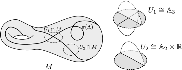
Figure 9. The case $d=2$. The neighborhood of a point in the front projection of the Legendrian $\Lambda$ is homeomorphic to either $\mathbb{A}_{2}\times\mathbb{R}=\mathbb{S}tar_{1}\times\mathbb{R}$ or $\mathbb{A}_{3}=\mathbb{S}tar_{2}$. Note that in general it is the star quivers $Star_{k}$ that appear, and not the $A_{k}$ series.

Similarly, around a singular point of $\pi(\Lambda)$ by the normal crossings condition, $U$ is homeomorphic to $\mathbb{R}^{d}$ with $k$ half-spaces glued along $k$ coordinate hyperplanes. Consider now the arboreal singularity $\mathbb{S}tar_{k}$ corresponding to the star quiver with $k$ leaves; this is homeomorphic to $\mathbb{R}^{k}$ with $k$ half-spaces glued along coordinate hyperplanes. By comparison we have a homeomorphism $U\simeq\mathbb{S}tar_{k}\times\mathbb{R}^{d-k}$. ∎

Thus $(\mathbb{X},\mu\operatorname{Sh}^{c}_{\mathbb{X}})$ is a locally arboreal space. We check that a sufficient criterion for its orientability is the orientability of the base manifold $M$.

Theorem 6.5.

The arboreal space $(\mathbb{X},\mu\operatorname{Sh}^{c}_{\mathbb{X}})$ admits an orientation if and only if $M$ is orientable; in that case it extends the orientation on $M$, i.e. which agrees with the given orientation on $M$ when restricted to the smooth locus of $\mathbb{X}$.

Proof.

Theorem 1.12 reduces us to consider $\mu\operatorname{Sh}=(\mu\operatorname{Sh}^{c})^{pp}$. There is an embedding $\mathcal{L}oc^{b}_{M}\hookrightarrow\mu\operatorname{Sh}$; in terms of the local models $U$, this identifies the locus $U\cap M$ with the disc corresponding to the root vertex $\rho$ of the quiver, and the embedding functor is the embedding of $\operatorname{Perf}$ as the subcategory spanned by the corresponding projective (and simple) object $P_{\rho}$.

This embedding is an isomorphism of sheaves of categories on the top-dimensional locus (away from the projection of $\Lambda$), and moreover the embedding of $M$ is a homotopy equivalence. Under the isomorphism induced in homology we have $w_{1}(\mathbb{X},\mu\operatorname{Sh}^{c}_{\mathbb{X}})=w_{1}(M,\mathcal{L}oc^{c})$, which vanishes if $M$ is orientable. ∎

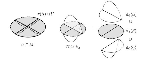
Figure 10. The coorientation of the front projection $\pi(\Lambda)$ defines a decomposition of $U\simeq\mathbb{A}_{3}$ into discs $\mathbb{A}_{3}(\alpha)$ labelled by each vertex of $A_{3}$. The choice of rooting is given by picking the center vertex of the quiver (which labels the disc along $M$) to be the root.

7. Examples

In this section we recall various categories which arise as the global sections of a sheaf or cosheaf of categories on an oriented locally arboreal space. As a consequence of our results, we conclude the existence of certain absolute and relative Calabi-Yau structures.

To relate this discussion to the subject of shifted symplectic geometry, we recall the following theorem.

Theorem 7.1.

[13, Thm.5.5] Let $C$ be a smooth dg category with a $d$-dimensional smooth Calabi-Yau structure. Then there is an induced $(2-d)$-shifted symplectic structure on its moduli space of objects $\mathcal{M}_{C}$. Moreover, if $f:C\leftrightarrows D:f^{r}$ is a continuous adjunction of smooth categories with a relative smooth Calabi-Yau structure on $f$ which is compatible with the (absolute) structure on $C$, the induced map $\mathcal{M}_{D}\to\mathcal{M}_{C}$ has a Lagrangian structure.

In the theorem above, $\mathcal{M}_{C}$ denotes the ‘moduli space of objects’ of $C$ as described in [94].

Remark.

There were similar results previously proven in the literature; in particular we have [93, Theorem 1.7] which proves the existence of the derived Lagrangian structure in the case that $\mathcal{A}$ and $\mathcal{B}$ are smooth and proper, which is not directly applicable to this paper since the categories of interest are smooth but not proper in general. Another result of relevance is [96, Theorem 1.19] which applies to dg categories “concentrated in non-negative degrees” and constructs shifted symplectic structures on their derived moduli of representations, which is the substack of the moduli $\mathcal{M}_{\mathcal{A}}$ representing objects of zero Tor amplitude.

Using the theorem above together with our result about orientations gives the following corollary.

Corollary 7.2.

Let $X$ be a stratified space with compact boundary $\partial X$, equipped with a locally saturated cosheaf $\mathcal{W}$. Then an orientation of dimension $d$ on $\mathcal{W}^{pp}$ determines a $(3-d)$-shifted symplectic structure on $\mathcal{M}_{\mathcal{W}(\partial X)}$ and a Lagrangian structure on the morphism $\mathcal{M}_{\mathcal{W}(X)}\to\mathcal{M}_{\mathcal{W}(\partial X)}$.

Therefore constructing orientations will then give rise to shifted symplectic structures, Poisson structures, quantizations, etc. in the appropriate circumstances [76, 14]. Direct application of our methods yield constructions in the “type A” cases; e.g. the moduli space for a point is $\mathcal{M}_{\operatorname{Perf}}$ inside which one can find the various $BGL_{n}$. We expect that the desired symplectic structures for the analogous moduli spaces for other groups can be constructed via Tannakian considerations as in [87, Sec. 6], but do not develop this in detail here.

Remark.

In this section to ease notation we will denote the moduli stack of objects using a blackboard bold capital to distinguish it from the category, e.g. the category of perfect complexes is denoted $\operatorname{Perf}$ and the moduli stack of perfect complexes is $\operatorname{\mathbb{P}\mathrm{erf}}=\mathcal{M}_{\operatorname{Perf}}$, same for local systems $\operatorname{Loc}$ and $\operatorname{\mathbb{L}\mathrm{oc}}$.

7.1. The associated graded of a filtration

Let $\mathbb{X}$ be a comb: a one-dimensional space formed as the union of $\mathbb{R}$ and the positive cone on some $n$ points $\{p_{i}\}$ at positive contact infinity. The category $\operatorname{Sh}_{\{p_{i}\}}(\mathbb{R})$ is equivalent to the category $\operatorname{\mathbb{F}\mathrm{ilt}}_{n}$ of $n$-step filtered perfect complexes, which just means sequences of perfect complexes

$$F_{0}\to F_{1}\to\ldots\to F_{n}.$$

Corollary 7.3.

The functor

$$\operatorname{Filt}_{n} \to \operatorname{Perf}^{\otimes(n+1)}\times\operatorname{Perf}$$

$$F_{0}\to\ldots\to F_{n} \mapsto (F_{0},Cone(F_{0}\to F_{1}),Cone(F_{1}\to F_{2}),\ldots,Cone(F_{n-1}\to F_{n})),\,F_{n}$$

has a relative proper Calabi-Yau structure, coming from an orientation of dimension 1, so the corresponding map of moduli spaces of objects

$$\operatorname{\mathbb{F}\mathrm{ilt}}\to\operatorname{\mathbb{P}\mathrm{erf}}^{\times(n+1)}\times\operatorname{\mathbb{P}\mathrm{erf}}$$

is a Lagrangian mapping to a $2$-shifted symplectic space.

Proof.

This follows immediately from Theorem 6.5. Alternatively, the fact that the comb is orientable follows from its being contractible. ∎

Remark.

Note that following the description in 6.5, the decomposition into “discs” (here intervals) is such that the boundary of the $i$th interval is given by the endpoints $(+\infty)-(p_{i})$, if we pick the positive orientation on the base manifold $\mathbb{R}$. So in the Lagrangian map of moduli stacks the first factor $\operatorname{\mathbb{P}\mathrm{erf}}^{\times(n+1)}$ is endowed with the opposite 2-shifted symplectic structure, where the last factor $\operatorname{\mathbb{P}\mathrm{erf}}$ has the usual 2-shifted symplectic structure.

Figure 11. The comb $\mathbb{X}$. We pick a decomposition of $\mathbb{X}$ into overlapping intervals; in this case the $i$th interval has endpoints $p_{i}$ and $+\infty$, and extending the positive orientation on $\mathbb{R}$, its boundary is $(+\infty)-(p_{i})$.

Restricting to the open substack $\operatorname{\mathbb{F}\mathrm{ilt}}_{n}^{\circ}$ where all $F_{i}$ and all $Cone(F_{i}\to F_{i+1})$ can be represented by vector spaces in degree zero, we see that the image of the morphism above in each factor $\operatorname{\mathbb{P}\mathrm{erf}}$ lands in some substack $\mathbb{B}GL_{m_{i}}\subset\operatorname{\mathbb{P}\mathrm{erf}}$, and moreover that each map $F_{i}\to F_{i+1}$ is injective. Denoting $m_{0}=\dim F_{0},m_{i}=\dim Cone(F_{i}\to F_{i+1})$ and $m=\dim F_{n}$, this implies that $m_{0}+\dots+m_{n}=m$. So $\operatorname{\mathbb{F}\mathrm{ilt}}_{n}^{\circ}$ splits into components labelled by collections of integers $m,\{m_{i}\}$, and each component has a 2-shifted Lagrangian morphism

$$\operatorname{\mathbb{F}\mathrm{ilt}}_{n}^{\circ}(m,\{m_{i}\})\to(\mathbb{B}GL_{m_{0}}\times\dots\times\mathbb{B}GL_{m_{n}})\times\mathbb{B}GL_{m},$$

which can be interpreted as a $2$-shifted Lagrangian correspondence between $\mathbb{B}GL_{m}$ and $\mathbb{B}L$ for the Levi subgroup corresponding to the partition $\{m_{i}\}$. This was originally shown in [81], where a Lagrangian correspondence

is used to define the “partial group-valued symplectic implosion”. Note that once we fix the decomposition $m=m_{0}+\dots+m_{n}$, we can identify the substack $\operatorname{\mathbb{F}\mathrm{ilt}}_{n}^{\circ}(m,\{m_{i}\})$ as the classifying space $\mathbb{B}P$ for the parabolic $P$ corresponding to $L$: a map from some other space $\mathbb{X}\to\operatorname{\mathbb{F}\mathrm{ilt}}_{n}^{\circ}(m,\{m_{i}\})$ determines an invariant filtration of the vector space $k^{m}$, therefore up to equivalence it is the data of a $P$-bundle over $\mathbb{X}$.

7.2. Invariant filtrations near punctures on surfaces

Let $\Sigma$ be an oriented surface with boundary consisting of $n$ circles; draw a collection of $m_{i}$ concentric circles at each boundary component, and choose co-orientations and therefore Legendrian lifts. Let $\Lambda$ denote the union of these lifts. Just as in the previous subsection, the corresponding category $Sh_{\Lambda}(\Sigma)$ amounts to the category of sheaves on $\Sigma$ with invariant filtrations at the punctures. Note that $\Lambda\cup\partial\Sigma$ is just a union of $m=\sum m_{i}$ circles.

Corollary 7.4.

The morphism $\operatorname{\mathbb{S}\mathrm{h}}_{\Lambda}(\Sigma)\to\operatorname{\mathbb{L}\mathrm{oc}}(\Lambda\cup\partial\Sigma)=\operatorname{\mathbb{L}\mathrm{oc}}(S^{1})^{\times m}$ is $1$-shifted Lagrangian.

Proof.

This follows immediately from Theorem 6.5. ∎

Again, we can take the substack $\operatorname{\mathbb{S}\mathrm{h}}_{\Lambda}(\Sigma)^{\circ}$ on which the restriction of the sheaf to $\Sigma$ has cohomology concentrated in degree zero; the resulting space is an Artin stack is the classical sense, and as in the comb example above, it has components labelled by the microlocal ranks along the boundary components; the morphism splits into components

$$\operatorname{\mathbb{S}\mathrm{h}}_{\Lambda}(\Sigma)^{\circ}(\{m_{i}\})\to\left[\frac{GL(m_{1})}{GL(m_{1})}\right]\times\dots\times\left[\frac{GL(m_{n})}{GL(m_{n})}\right],$$

where the stacky quotient is taken with respect to the adjoint action.

To get a space with a symplectic structure, one can choose correspondingly another $1$-shifted Lagrangian morphism to the moduli space of local systems around the boundary, and performing Lagrangian intersection between the two $1$-shifted Lagrangians as in [80] this gives a $0$-shifted symplectic space.

Corollary 7.5.

The moduli space of local systems on a surface equipped with invariant filtrations at the punctures, of which the conjugacy classes $C_{i}$ of the associated graded holonomies are pre-specified, carries a $0$-shifted symplectic structure.

Proof.

As in Safronov [80], this can be deduced from Corollary 7.4 (which has a different proof in that paper) by observing that fixing a conjugacy class $C$ in a reductive group $G$ determines a Lagrangian morphism $[\frac{C}{G}]\to[\frac{G}{G}]$. Performing Lagrangian intersection between $\operatorname{\mathbb{S}\mathrm{h}}_{\Lambda}(\Sigma)^{\circ}(\{m_{i}\})$ and $[\frac{C_{1}}{GL(m_{1}}]\times\dots\times[\frac{C_{n}}{GL(m_{n})}]$ gives the symplectic structure on the moduli space with prescribed holonomies. ∎

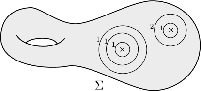
Figure 12. On the surface $\Sigma$ with two punctures, and with fixed microlocal rank along the concentric circles of $\Lambda$. If we look at the substack of $Sh_{\Lambda}(\Sigma)$ of objects with rank 0 at the punctures, the microlocal rank conditions mean we have rank 3 local systems equipped with invariant filtrations near each puncture; in this particular case we have two filtrations respectively of the form $0\subset k\subset k^{2}\subset k^{3}$ and $0\subset k\subset k^{3}$

Example.

Consider $\Sigma$ an oriented surface with boundary $\partial\Sigma=$ union of $n$ circles, without any Legendrians. The Artin stack $\operatorname{\mathbb{S}\mathrm{h}}(\Sigma)^{\circ}$ has disjoint components $\operatorname{\mathbb{L}\mathrm{oc}}_{GL(m)}(\Sigma)$ labelled by the rank $m$ of the local system, and so we have 1-shifted Lagrangian morphisms

$$\operatorname{\mathbb{L}\mathrm{oc}}_{GL(m)}(\Sigma)\to(\operatorname{\mathbb{L}\mathrm{oc}}_{GL(m)}(S^{1}))^{\times n}=\left[\frac{GL(m)}{GL(m)}\right]^{\times n}$$

and picking $n$ conjugacy classes $C_{i}$ in $G$, we can perform the intersection and get the so-called “tame” character variety of $\Sigma$.

Example.

Take $\Sigma$ to be the open cylinder with $n$ concentric circles around one of the boundary components, and no circles around the other. Fixing the ranks $m=m_{1}+\dots+m_{n}$ at each boundary, we get a 1-shifted Lagrangian morphism

$$\operatorname{\mathbb{S}\mathrm{h}}_{\Lambda}(\Sigma)^{\circ}\to\operatorname{\mathbb{L}\mathrm{oc}}_{GL_{m}}(S^{1})\times\operatorname{\mathbb{L}\mathrm{oc}}_{GL_{m_{1}}}(S^{1})\times\dots\times\operatorname{\mathbb{L}\mathrm{oc}}_{GL_{m_{n}}}(S^{1})=\left[\frac{G}{G}\right]\times\left[\frac{L}{L}\right],$$

where $L$ is the Levi subgroup corresponding to the partition $\{m_{i}\}$. This example also appears in [81], as a 1-shifted Lagrangian correspondence

where the identification of our space with $[\frac{P}{P}]$ comes from the observation that an invariant filtration on $\Sigma$ is the same data as a $P$-local system on $S^{1}$.

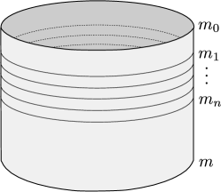
Figure 13. The restriction to the upper boundary components can be assembled into a map to $[\frac{L}{L}]$ where $L$ is a Levi subgroup of $G=GL_{m}$ given by the integers $\{m_{i}\}$. The restriction to the lower boundary components is a map to $[\frac{G}{G}]$ giving the monodromy of the $G$-local system

Another way of deducing this particular case is by writing $\Sigma$ as the product of a circle and a comb (as in 7.1). Therefore we have an equivalence of derived stacks

$$\operatorname{\mathbb{S}\mathrm{h}}_{\Lambda}(\Sigma)=\mathbb{R}Map(S^{1},\operatorname{\mathbb{F}\mathrm{ilt}}_{n})$$

and the Lagrangian correspondence is obtained from the correspondence in section 7.1 by applying the mapping stack functor $\mathbb{R}Map(S^{1},-)$, which shifts the degree down to the 1-shifted Lagrangian correspondence above.

Remark.

In the rank one case, when $k_{i}=1$, the correspondence $[\frac{B}{B}]\to[\frac{G}{G}]\times[\frac{T}{T}]$ is a group version of the Grothendieck-Springer correspondence, and we have $[\frac{B}{B}]\simeq[\frac{\tilde{G}}{G}]$ where $G$ acts on the Springer resolution $\tilde{G}$ by conjugation.

7.3. Stokes filtrations near punctures on surfaces

Rather than take an invariant filtration around a puncture, one can allow the filtration itself to undergo monodromy. The resulting notion generalizes the notion of Stokes structure; we will call it a Stokes filtration. In most works, this was presented as suggested above: in terms of a sheaf on the boundary circle equipped with a filtration that itself varies. This notion can be found e.g. in [64]. Defining what precisely it means for a filtration to vary along a circle is nontrivial and somewhat mysterious at the points where the steps in the filtration cross.

We prefer to turn this notion sideways: rather than a filtered sheaf on $S^{1}$ with varying filtration, we take a sheaf on $S^{1}\times\mathbb{R}$ with microsupport in a prescribed Legendrian braid closure. This determines a filtration in the $\mathbb{R}$ direction, just as in the previous examples; as it happens, the above notion exactly captures at the crossings the notion in [64] of Stokes filtration. This idea seems to have been known to the experts, but we have not found any systematic exposition of it in the classical literature.

We made some attempt in this direction in [85, Sec. 3.3]. Here we simply recall that the Deligne-Malgrange account of the irregular Riemann-Hilbert correspondence on Riemann surfaces can be formulated as follows. Suppose we are given a Riemann surface $\Sigma$ with marked points $p_{i}$, and a specification of a (possibly ramified) irregular type $\tau_{i}$, i.e., formal equivalence class of irregular singularity, at each. Then there is an associated Legendrian link $\Lambda=\coprod\Lambda(\tau_{i})$, a union of links localized near the $p_{i}$, and an equivalence of categories between the irregular connections with these singularities, and the full subcategory of $\operatorname{Sh}_{\Lambda}(\Sigma)$ on objects which have cohomology concentrated in degree zero, and appropriate rank stalks and microstalks. The corresponding component of the moduli space is the moduli space of Stokes data. Finally, the microlocal restriction morphism $\operatorname{Sh}_{\Lambda}(\Sigma)\to\operatorname{Loc}(\Lambda)$ is what would have classically been called “taking the formal monodromies”.

Corollary 7.6.

The morphism from a moduli space of Stokes data to the moduli space of formal monodromies is 1-shifted-Lagrangian.

Corollary 7.7.

A moduli space of Stokes data with formal monodromies taking values in prescribed conjugacy classes is 0-shifted-symplectic. In particular, any open substack which happens to be a scheme is symplectic in the usual sense.

This recovers and generalizes all constructions of symplectic structures in e.g. [8, 9, 11, 66] for $GL_{n}$ connections.

Example.

(Wild character variety) Consider a disc $\Sigma$ punctured at the origin and a trivial rank $n$ vector bundle $E\to\Sigma$, where the origin is marked with the irregular type

$$Q(z)=\frac{A}{z^{r}},\qquad r\in\mathbb{Z}_{+},A\in\mathfrak{t}^{reg}\subset\mathfrak{gl}_{n}$$

i.e., $A$ has all distinct eigenvalues. A meromorphic connection $\nabla$ on $E$ has this irregular type if it can be brought by a local analytic gauge transformation to the connection defined by the connection one-form $dQ$.

By the irregular Riemann-Hilbert correspondence, the category of meromorphic connections on the trivial vector bundle with this irregular type is equivalent to the category of Stokes data. From the Stokes data, one can recover the monodromy of $\nabla$ and the formal monodromy; this latter is an element of the centralizer $Z_{G}(A)$ (in this case, the maximal torus $T$) up to conjugation.

The moduli of Stokes data with fixed monodromies and formal monodromies is commonly known as the wild character variety. Upon fixing conjugacy classes $C_{G},C_{T}$ in $G$ and $T$, the wild character variety can be described as a quasi-Hamiltonian quotient [9, 10]

$$(G\times T\times(U_{+}\times U_{-})^{r})\mathbin{/\mkern-6.0mu/}_{C_{G},C_{T}}(G\times T)$$

where $U_{\pm}$ are the unipotent subgroups corresponding to the maximal torus $T$. The moment map to $G$ is taking the monodromy around the singularity, and the map to $T$ is taking the formal monodromy.

In our description, this category of Stokes data becomes a full subcategory of the category $Sh_{\Lambda}(\Sigma)$ of microlocal sheaves, for a corresponding Legendrian link $\Lambda\subset T^{\infty}$ around the singularity. The monodromy and formal monodromy then become literal monodromies of the local systems one gets by restriction to the boundary. To explicitly construct $\Lambda$, one can follow the prescriptions in [85, Sec. 3.3]. This can be heuristically stated in terms of the asymptotics of flat sections, i.e. the growth behavior of the solutions to

$$\frac{df}{dz}=\frac{dQ}{dz}f(z).$$

In this case, the solutions are spanned by $n$ different solutions $f_{i}\sim\exp(\lambda_{i}z^{-r})$, where $\lambda_{i}$ are the eigenvalues of $A$, and we only keep the exponential part of the asymptotics. The Stokes phenomenon refers to the fact that these corresponds to asymptotics of solutions in different sectors; as we go from one sector to the other, the growth of these solutions changes. On each sector, we draw concentric strands for the $f_{i}$, ordering them by growth: the faster-growing ones further from the origin. Whenever we cross a Stokes ray, where the solutions $f_{i},f_{j}$ switch growth asymptotics, we introduce a crossing between the $i$ and $j$ strands.

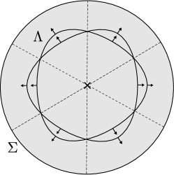
Figure 14. The Legendrian link for the irregular type $\left(\begin{smallmatrix}1&0\\ 0&1\end{smallmatrix}\right)$ $\frac{1}{z^{3}}$. The Legendrian link $\Lambda\subset T^{\infty}\Sigma$ is obtained by lifting the projection using the outward coorientation. The dashed lines are the Stokes rays, where the asymptotics of formal solution changes. Note that each component of the link is unknotted with itself: this is true of all the examples of this form.

In the case we described above ($A\in\mathfrak{t}^{reg}$), the corresponding Legendrian link $\Lambda$ is the closure of a $(n,2r)$ braid , cooriented outward, where we enforce the condition that the rank of the stalk inside $\Lambda$ is zero, and the microlocal ranks on each component of $\Lambda$ is one. What we call the moduli of Stokes data $\mathcal{M}_{\Lambda}$ is the moduli of objects in the full subcategory of $Sh_{\Lambda}(\Sigma)^{\circ}$ with those rank conditions. The maps given by restriction to the boundary components can be assembled into a 1-shifted Lagrangian map

$$\mathcal{M}_{\Lambda}\to\left[\frac{G}{G}\right]\times\left[\frac{T}{T}\right]$$

where $[\frac{G}{G}]$ is $G$-local systems on the boundary of the disc, and $[\frac{T}{T}]$ is rank one local systems on $\Lambda$. In this description, taking quasi-Hamiltonian quotient corresponds to taking intersection with another Lagrangian $[\frac{C_{G}}{G}]\times[\frac{C_{T}}{T}]$. The explicit description of the moduli space $\mathcal{M}_{\Lambda}$ can be obtained by following the prescriptions in [86]; one can check that this stack can in fact be expressed as the quotient $[(G\times T\times(U_{+}\times U_{-})^{r})/(G\times T)]$, agreeing with the previously existing description.

Example.

With the same notation of the previous example, consider the irregular type

$$Q=\frac{A}{z^{r/2}},\qquad A\in\mathfrak{t}^{reg}\subset\mathfrak{gl}_{n}$$

where $r$ is some odd number. Following the discussion in the last example, we get $n$ solutions $f_{i}\sim\exp(\lambda_{i}z^{-r})$ The strands $i$ and $j$ will cross whenever $f_{i}$ and $f_{j}$ “switch” growth asymptotics. Suppose for instance that $\lambda_{i},\lambda_{j}\in\mathbb{R}$. Writing $z=Re^{i\theta}$ the asymptotics will switch whenever $Re(z^{-r/2})=0$, i.e. on the rays

$$\theta=\frac{\pi}{r}+\frac{2n\pi}{r}.$$

There are $r$ such rays between any pair $i,j$ even if $\lambda_{i},\lambda_{j}\notin\mathbb{R}$: the expression for the rays is more complicated by the number of rays doesn’t change. Therefore $\Lambda$ is the closure of a $(n,r)$ braid.

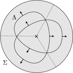
Figure 15. The Legendrian link for the irregular type $\left(\begin{smallmatrix}1&0\\ 0&1\end{smallmatrix}\right)$ $\frac{1}{z^{3/2}}$. The microlocal rank on the link $\Lambda$ is 1.

The case where $n=2,r=3$ gets us a trefoil and appears in Stokes’ discussion of the Airy equation [89]. Note that the trefoil has only one component, so the formal monodromy map lands in $Loc_{k^{*}}(S^{1})\simeq[\frac{k^{*}}{k^{*}}]$ which doesn’t stand for $\frac{T}{T}$ for any maximal torus $T\subset GL_{2}$. This explains why this more general case cannot be described just in terms of moment maps into subgroups of $G$.

Remark.

One can play many variations on the theme of Stokes filtrations and irregular singularities. Considering connections with matrices $A$ that are not in the regular locus of $\mathfrak{g}$, it becomes necessary to look at further less singular terms in the expression for $dQ$. To find the corresponding Legendrians one can still follow the prescriptions in [85]. One obtains cablings of torus knots by other torus knots and cablings of torus knots by such cablings and so on.

But there are many other knots that one can consider: pick any positive braid and close it around the origin into a Legendrian $\Lambda$. Picking rank conditions and monodromies around the components of $\Lambda$, this gives a symplectic space $\mathcal{M}_{\Lambda}$ that doesn’t necessarily come from an irregular meromorphic singularity. We can expect these spaces to carry some of the same structures as the tame and wild character varieties; whether this is true remains a topic of future research.

Remark.

For moduli of Stokes data for connections on higher dimensional complex varieties, the corresponding Riemann-Hilbert theorem recently been proven [2]. We expect that it can be reformulated into an analogous “microsupport in certain smooth Legendrians” version, from which we would be able to immediately deduce the existence of the shifted symplectic structure.

7.4. Positroid varieties, multiplicative Nakajima varieties, and other cluster structures

The combinatorics of cluster algebras arising from surfaces was originally organized around data given variously as a graph on a surface, a triangulation on a surface, etc [78, 29, 38, 39, 30]. One presentation of this data is in terms of the so-called “alternating strand diagram”, the manipulation of which by combinatorial topology [90] underlies various theorems of the cluster algebra.

In [85], we took the perspective that the alternating strand diagram should be viewed as a Legendrian knot, that triangulations of the surface give rise to Lagrangian fillings of it, and that all the corresponding cluster algebraic formulas are computing the Floer homology between such fillings. In particular, the corresponding cluster $X$-variety was identified as a moduli space of “rank one” objects in $Sh_{\Lambda}(\Sigma)$, where $\Lambda$ is the Legendrian lift of the alternating strand diagram, and $\Sigma$ is the base curve.

In [84], we took a slightly different perspective: rather than work from $\Sigma,\Lambda$, we began with a Legendrian $L$ — one could view it as one of the above-mentioned fillings of $\Lambda$ — and attached Weinstein handles to its cotangent bundle along Legendrians which project to simple closed curves. This perspective is yet more general than the previous.

It includes as a special case the multiplicative Nakajima quiver varieties of [20, 95, 6]; this being the case where the attaching circles are contractible. Indeed, this case is very close to the presentation in [6]. In that reference, rather than locally arboreal singularities, they consider the spaces which are locally either a smooth surface or modeled on the Lagrangian singularity given by the union of the zero section and the conormal to point. However, this local model admits a noncharacteristic deformation to the union of the zero section and the positive conormal to a circle. The deformation is just given by the contact isotopy induced by the Reeb flow.

Thus, the present work recovers all constructions of symplectic and Poisson structures on such spaces. It will be interesting to investigate how the deformation quantization formalism of [14] interacts with these notions.

7.5. The augmentation variety of knot contact homology

Consider a knot or link $K\subset S^{3}$. Naturally associated to this is the category of sheaves constructible with respect to the stratification $S^{3}=K\cup S^{3}\setminus K$. This study of this category e.g. allows one to prove that the Legendrian isotopy type of the conormal torus to a knot determines the knot [82, 25]. In an appropriate sense, it is equivalent to the a category of augmentations of knot contact homology.

The union of the conormal to the knot with the zero section is not arboreal, but as the above discussion of [6], this can be remedied by perturbing the conormal torus by the Reeb flow, resulting in a skeleton given by the union of the zero section and the positive conormal to the inward (or outward) co-oriented boundary of a tubular neighborhood of the knot.

In any case, we can study the space of objects in this category. It has a map to the category of local systems on $T^{2}$, which by the results here, becomes a $0$-shifted Lagrangian morphism on moduli spaces. We note that the study of this moduli space was also suggested in [6].

To select a connected component (indeed, the connected component corresponding to what is usually called the augmentation variety), we can pick those sheaves whose microsupport on the conormal torus is rank one in degree zero, i.e., what are called simple sheaves in [55]. We restrict further to the open locus on which objects which have no global sections, the main point of which is to eliminant constant summands. Let us write $A_{1}(K)$ for this component.

Restriction to the microlocal boundary gives a map $A_{1}(K)\to\operatorname{Loc}_{k^{*}}(T^{2})=(k^{*})^{2}$. There is an analogous map in knot contact homology, described in [74, 24, 1]. Note that objects in $A_{1}(K)$ are easy to understand: they are a local system in the complement of $K$, which is extended by a codimension one subspace of meridian invariants along $K$; or possibly a nontrivial rank one local system supported on $K$.

From this point of view it is clear both why $A_{1}(K)$ contains the classical $A$-polynomial curve, and also what are the other components: the $A$ polynomial curve has to do with $SL_{2}$ representations of the fundamental group; any such becomes, after rescaling by an eigenvalue of the meridian, a $GL_{2}$ representation with a meridian invariant subspace. Similarly it is clear what the other components of $A_{1}(K)$ are. (Compare [17] for direct proofs of the analogous statements about the augmentation variety, from which it can be deduced that $A_{1}(K)$ as described here is the augmentation variety of knot contact homology.)

Thus we have shown that the morphism $A_{1}(K)\to k^{*}\times k^{*}$ is (0-shifted) Lagrangian. This morphism can be quantized either by the formal methods of [14] or using higher genus holomorphic curves [1, 26, 27]; it should be interesting to compare these approaches.

8. The diagonal cosheaf

In these next two sections, we will prove the statements made in the introduction about orientations on ccc spaces with smooth cosheaves. Let us now explain why this case is more technically challenging than the corresponding results for csc spaces; this is the reason for delaying the proofs until now.

In treating duality for sheaves of categories, we were able to avoid directly working with bimodules by evaluating at pairs of objects. Indeed, in the sheaf case, given $x,y\in\mathcal{F}(U)$, we have that $\operatorname{Hom}_{\mathcal{F}(U)}(x,y)$ is itself the global sections of a sheaf on $U$. Using the compatibility between evaluations, limits and right duals allowed us to formulate the nondegeneracy condition simply in terms of these sheaves.

The lack of a useful analogue in the cosheaf case — and beyond this the fact that the evaluation maps do not interact in a simple way with taking colimits of bimodules or with taking left duals — mean that we must directly with bimodules. To do so we will require a notion of the ‘cosheaf of diagonal bimodules over a given cosheaf of categories’. Dealing with this will require some $(\infty,2)$-categorical machinery from [44, 45].

After establishing the existence and property of this cosheaf of diagonal bimodules, we will not need to think about $(\infty,2)$-categories any more.

So let us now summarize the results of this section. In [44] is constructed an $(\infty,1)$-category named $\operatorname{End}(\operatorname{DGCat})$ whose objects are given by a pair $(\mathcal{A},\mathcal{M})$ of an object $\mathcal{A}$ of $\operatorname{DGCat}$ and a bimodule $\mathcal{M}\in\mathcal{A}\mathchar 45\relax\operatorname{Mod}\mathchar 45\relax\mathcal{A}$. The role of the $(\infty,2)$ machinery in [44] is to give a concise presentation of the higher structures of $\operatorname{End}$. Here we will use it similarly to construct the following structure:

Theorem 8.1.

There is a colimit preserving $(\infty,1)$-functor

$$\Delta:\operatorname{dgcat}\to\operatorname{End}(\operatorname{DGCat}),$$

which on objects is given by mapping a category $\mathcal{A}$ to the pair $(\mathcal{A},\operatorname{Id}_{\mathcal{A}})$.

Remark.

There is no analogous map $\Delta:\operatorname{DGCat}\to\operatorname{End}(\operatorname{DGCat})$, because the morphisms in $\operatorname{End}(\operatorname{DGCat})$ all come from right dualizable morphisms in $\operatorname{DGCat}$, i.e. morphisms in $\operatorname{dgcat}$. (See Proposition 8.8.)

Corollary 8.2.

(Def. 8.22) Given a space $X$ and a $\operatorname{dgcat}$-valued cosheaf $\mathcal{F}$ on $X$, by composition with $\Delta$ we obtain an $\operatorname{End}(\operatorname{DGCat})$-valued cosheaf $\Delta\mathcal{F}$. We term this the diagonal cosheaf.

Given an $\operatorname{End}(\operatorname{DGCat})$ cosheaf, composing with the corestriction maps and their adjoints, we may extract a cosheaf valued in bimodules over the global sections, which we describe it at the level of objects.Let $U\mapsto(\mathcal{F}(U),\mathcal{M}(U))$ be such a cosheaf; and for $U\subset V$ let us denote $\phi^{V}_{U}:\mathcal{F}(U)\to\mathcal{F}(V)$ the part of the corestriction map corresponding to $\mathcal{F}$. Then we show that for any open $V$ there is a $\operatorname{End}(\mathcal{F}(V))$-valued cosheaf which assigns $U\mapsto\phi^{V}_{U}\circ\mathcal{M}(U)\circ(\phi^{V}_{U})^{r}$, where we regard the bimodule $\mathcal{M}(U)$ as an endomorphism of $\mathcal{F}(U)$, and $(-)^{r}$ denotes the right adjoint. We will be interested in this later only for the diagonal cosheaf, from which we obtain:

Corollary 8.3.

(Lem. 8.20, Def. 8.23) For any $U\subset V$ as above, there is an $\operatorname{End}(\mathcal{F}(V))$-valued cosheaf $\Delta\!\!\!\!\Delta(\mathcal{F}|_{V})$ on $V$ which assigns

$$U\mapsto\phi^{V}_{U}\circ(\phi^{V}_{U})^{r}.$$

Moreover, for any inclusion of opens $V\subset V^{\prime}$ we have a natural equivalence

$$(\phi^{V^{\prime}}_{V})^{r}\circ\Delta\!\!\!\!\Delta(\mathcal{F}|_{V})\circ\phi^{V^{\prime}}_{V}\cong\Delta\!\!\!\!\Delta(\mathcal{F}|_{V^{\prime}})$$

of $\operatorname{End}(\mathcal{F}(V^{\prime}))$-valued cosheaves on $V^{\prime}$.

8.1. Endomorphisms in $(\infty,2)$-categories

In this subsection we review ideas of [44, 45] regarding the construction of endomorphism categories and traces. Using similar ideas we construct certain variants we require in the sequel.

8.1.1. Modeling $(\infty,n)$-categories

Recall that an $(\infty,n)$ category is a higher category where all morphisms of dimension above $n$ are invertible; the usual ‘$\infty$-categories’ being the $(\infty,1)$-categories. In the literature there are many approaches to describe such structures; as we will use constructions from [44, 45], we follow them in modelling $(\infty,n)$-categories using Barwick’s $n$-fold complete Segal spaces [3]. Comparison theorems to other models can be found in [4].

Writing $\Delta$ for the simplicial indexing category, a $n$-fold complete Segal space $\mathcal{C}$ can be described by a collection of spaces $\mathcal{C}_{\vv k}$ indexed by vectors $\vv k\in\Delta^{n}$, with appropriate morphisms and coherence data between them; for any $0\leq p\leq n$, one should regard the space $\mathcal{C}_{(p)}$, where $(p)$ is the vector $(1,1,\dots,1,0,0,\dots)$ with $p$ entries ‘1’ followed by $(n-p)$ entries ‘0’, as the space of $p$-morphisms of the $(\infty,n)$-category $\mathcal{C}$. For $\vv k\in\Delta^{p}$ we can define a $p$-fold complete Segal space $\iota_{p}\mathcal{C}$ given by

$$(\iota_{p}\mathcal{C})_{\vv k}:=\mathcal{C}_{\vv k,0,\dots,0}$$

modeling the maximal $(\infty,p)$-subcategory of $\mathcal{C}$.

Barwick constructs the category $n$-fold complete Segal spaces as a certain localization of the category of presheaves of spaces over $\Delta^{n}$; we denote his category as $\mathrm{CSS}(\Delta^{n})$. This category gives a model for the homotopy theory of $(\infty,n)$-categories [3, Corollary 14.3 and Theorem 14.6]. In particular, strict $n$ categories certainly give objects of $\mathrm{CSS}(\Delta^{n})$.

Let us recall some objects of $\mathrm{CSS}(\Delta^{n})$ that will play an important role later.

Definition 8.4.

The walking $i$-morphism, or $i$-globe, $\Theta^{(i)}$ [4, 45]. Inductively define $\Theta^{(i)}$ as a strict $i$-category, by setting $\Theta^{(i)}$ to be the singleton set, and $\Theta^{(i)}$ to be the category with two objects $\{0,1\}$ and with morphisms given by

$$\operatorname{Hom}_{\Theta^{(i)}}(x,y)=\begin{cases}\Theta^{(0)},&\text{if }x=y\\ \Theta^{(i-1)},&\text{if }x=0,y=1\\ \varnothing,&\text{if }x=1,y=0,\end{cases}$$

with the unique composition law giving a strict $i$-category. This category has the property that for any $(\infty,n)$-category $\mathcal{C}$ there is a canonical homotopy equivalence

$$\mathcal{C}_{(i)}\simeq\operatorname{maps}^{h}(\Theta^{(i)},\mathcal{C})$$

expressing the fact that $\Theta^{(i)}$ represents $i$-morphisms. For small values of $i$ we draw these categories as

$$\Theta^{(0)}=\bullet,\qquad\Theta^{(1)}=\leavevmode\hbox to68.57pt{\vbox to11.11pt{\text{[drawing]}}},\qquad\Theta^{(2)}=\leavevmode\hbox to68.57pt{\vbox to36.96pt{\text{[drawing]}}} \bullet \bullet \bullet \bullet \bullet \bullet \bullet \bullet$$

where we denote a 2-morphism by a double arrow and so on. Note that $\Theta^{(1)}=\Delta^{1}$ is the 1-simplex.

We will also need the walking $i$-by-$j$ morphisms of [45, Section 3]. These $\Theta^{(i);(j)}$ are defined inductively and are used by the authors of that paper to define the notion of (op)lax natural transformations. When $i$ or $j$ is zero we obtain the globe objects above: $\Theta^{(0);(i)}=\Theta^{(i);(0)}=\Theta^{(i)}$. The only space $\Theta^{(i);(j)}$ that we will need to use explicitly are drawn below.

Definition 8.5.

$$\Theta^{(1);(1)}=\leavevmode\hbox to68.57pt{\vbox to68.02pt{\text{[drawing]}}} \bullet \bullet \bullet \bullet \bullet \bullet \bullet \bullet$$

Using these objects, let us define the following two objects of $\mathrm{CSS}(\Delta^{n})$ (for some $n\geq 2$) by giving them as (homotopy) colimits in $\operatorname{CSS}(\Delta^{n})$.

Definition 8.6.

The object $\mathbb{S}$ of $\mathrm{CSS}(\Delta^{n})$ is given by the following colimit:

$$\mathbb{S}=\operatorname*{colim}\left(\Theta^{(0)}\leftarrow\Theta^{(0)}\sqcup\Theta^{(0)}\hookrightarrow\Theta^{(1)}\right)=\operatorname*{colim}\left(\bullet\quad\leftarrow\quad\leavevmode\hbox to11.67pt{\vbox to39.56pt{\text{[drawing]}}}\quad\hookrightarrow\quad\leavevmode\hbox to11.67pt{\vbox to39.56pt{\text{[drawing]}}}\right) \bullet \bullet \bullet \bullet \bullet \bullet \bullet \bullet$$

where $\hookrightarrow$ denotes the inclusion of the boundary points of the arrow $\Theta^{(1)}$.

This (homotopy) colimit is to be taken in $\operatorname{CSS}(\Delta^{n})$; as it is defined as a colimit, it is easy to calculate maps out of this category.

Remark.

The name for this object comes from considering the colimit simply taken in simplicial spaces, which would suggest:

$$\mathbb{S}\dashrightarrow\leavevmode\hbox to54.13pt{\vbox to51.78pt{\text{[drawing]}}} \bullet \bullet$$

This diagram does not portray a complete Segal space; the circle cannot be endowed with a composition rule that would satisfy the Segal condition. Nevertheless in $\mathrm{CSS}(\Delta^{n})$ one in fact has an identification $\mathbb{S}\simeq B\mathbb{N}$, with the $\infty$-category with one object and morphism given by the monoid $\mathbb{N}$ – which does have the appropriate composition rule.

8.1.2. Oplax natural transformations

We will follow the exposition in [44, Section 2.2], mostly borrowing notation from it. Given a complete $n$-fold Segal space $\mathcal{C}$ and a tuple $\vv k\in\Delta^{n}$ of natural numbers, there is a complete $n$-fold Segal space $\mathrm{Lax}_{\vv k}(\mathcal{C})$, defined using the walking morphisms [45, Definition 5.14]:

$$\left(\mathrm{Lax}_{\vv k}(\mathcal{C})\right)_{\vv l}:=\operatorname{maps}^{h}(\Theta^{\vv k,\vv l},\mathcal{C}).$$

For a fixed $\vv k$, these spaces for all $\vv l\in\Delta^{n}$ assemble into the complete $n$-fold Segal space $\mathrm{Lax}_{\vv k}(\mathcal{C})$ [45, Theorem 5.11]. In particular, for $\vv k=(p),\vv l=(0)$, we have an isomorphism

$$\left(\mathrm{Lax}_{(p)}(\mathcal{C})\right)_{(0)}\simeq\operatorname{maps}^{h}(\Theta^{(p)},\mathcal{C})=\mathcal{C}_{(p)},$$

exhibiting the space of objects of $\mathrm{Lax}_{(p)}(\mathcal{C})$ as the space of $p$-morphisms of $\mathcal{C}$. The corresponding morphisms can be understood as (higher) oplax natural transformations in $\mathcal{C}$.

Given two complete $n$-fold Segal spaces $\mathcal{B},\mathcal{C}$, [45, Corollary 5.19] defines another complete $n$-fold Segal space $\operatorname{Fun}^{\mathrm{oplax}}(\mathcal{B},\mathcal{C})$ (of ‘oplax transfors’) whose $\vv k$ space is given by

$$\operatorname{Fun}^{\mathrm{oplax}}(\mathcal{B},\mathcal{C})_{\vv k}=\operatorname{maps}^{h}(\mathcal{B},\mathrm{Lax}_{\vv k}(\mathcal{C})),$$

where $\operatorname{maps}^{h}$ denotes a strictly functorial model for the derived mapping space between presheaves of spaces. This complete $n$-fold Segal space $\operatorname{Fun}^{\mathrm{oplax}}(\mathcal{B},\mathcal{C})$ is functorial on the choice of $\mathcal{B},\mathcal{C}$.

These constructions can also be extended to incorporate symmetric monoidal structures. If $\mathcal{C}$ is a symmetric monoidal complete $n$-fold Segal space then $\mathrm{Lax}_{\vv k}(\mathcal{C})$ also carries a natural symmetric monoidal structure. If $\mathcal{B},\mathcal{C}$ are symmetric monoidal complete $n$-fold Segal spaces, then there is also a complete $n$-fold Segal space $\operatorname{Fun}^{\mathrm{oplax}}_{\otimes}(\mathcal{B},\mathcal{C})$ satisfying

$$\operatorname{Fun}^{\mathrm{oplax}}_{\otimes}(\mathcal{B},\mathcal{C})_{\vv k}=\operatorname{maps}^{h}_{\otimes}(\mathcal{B},\mathrm{Lax}_{\vv k}(\mathcal{C})),$$

where the subscript $\otimes$ means to consider symmetric monoidal maps [45, Corollary 6.9]. Again, this construction is functorial on the choice of $\mathcal{B},\mathcal{C}$.

8.1.3. Endomorphism categories

Let $\mathcal{C}$ be a complete $n$-fold Segal space, for some $n\geq 2$. We will denote by $\mathcal{C}^{\mathrm{rig}}$ the underlying $(\infty,n)$-category spanned by the dualizable objects in $\mathcal{C}$ (due to the symmetric monoidal condition, the left- and right-dualizable conditions agree). The functor $(-)^{\mathrm{rig}}$ preserves limits [61, Remark 4.6.1.11] and admits a left adjoint [44, Sec.2.2]

$$\mathrm{Fr}^{\mathrm{rig}}:\operatorname{Cat}_{(\infty,n)}\longleftrightarrow\operatorname{Cat}^{\otimes}_{(\infty,n)}:(-)^{\mathrm{rig}},$$

which from any $(\infty,n)$-category $\mathcal{C}$ gives a ‘free rigid symmetric monoidal $(\infty,n)$-category’ $\mathrm{Fr}^{\mathrm{rig}}(\mathcal{C})$.

Definition 8.7.

Consider the following $(\infty,n-1)$-categories:

$$\mathcal{C}^{\mathrm{RR}} =\iota_{n-1}\operatorname{Fun}^{\mathrm{oplax}}_{\otimes}(\mathrm{Fr}^{\mathrm{rig}}(\mathrm{pt}),\mathcal{C})\quad\text{``right-rigid subcategory''}$$

$$\operatorname{End}(\mathcal{C}) =\iota_{n-1}\operatorname{Fun}^{\mathrm{oplax}}_{\otimes}(\mathrm{Fr}^{\mathrm{rig}}(\mathbb{S}),\mathcal{C})\quad\text{``endomorphisms''}$$

Remark.

The definition above of the category $\operatorname{End}(\mathcal{C})$ is from [44], where $\mathbb{S}$ is denoted $B\mathbb{N}$ because the category $\mathbb{S}$ models the classifying category of the monoid of natural numbers. Since we will be using its explicit colimit presentation we will continue to call it $\mathbb{S}$. Further properties of $\operatorname{End}(\mathcal{C})$ can be found in [44].

Let us now describe these categories more explicitly.

Proposition 8.8.

When $\mathcal{C}$ is an $(\infty,2)$-category, at the level of homotopy categories, we have the following identifications

• The category $\mathcal{C}^{\mathrm{RR}}$ has as objects the dualizable objects $A$ of $\mathcal{C}$, and as morphisms between $A$ and $B$ the right-dualizable morphisms between $A$ and $B$ in $\mathcal{C}$.

• [44] The category $\operatorname{End}(\mathcal{C})$ has as objects pairs $(A,f)$, where $A$ is a dualizable object of $\mathcal{C}$ and $f$ is an endomorphism of $A$. The morphisms between $(A,f)$ and $(B,g)$ are pairs $(\phi,\alpha)$, such that $\phi$ is a right-dualizable morphism $A\to B$ and $\alpha:\phi\circ f\Rightarrow g\circ\phi$ is a 2-morphism in $\mathcal{C}$.

All the descriptions above are “up to equivalence” (i.e., given by pairs up to equivalence of pairs, etc.)

Proof.

We will start by describing the category $\mathcal{C}^{\mathrm{RR}}$. The space of objects is given by

$$\left(\mathcal{C}^{\mathrm{RR}}\right)_{(0)}=\operatorname{Fun}^{\mathrm{oplax}}_{\otimes}(\mathrm{Fr}^{\mathrm{rig}}(\mathrm{pt}),\mathcal{C})_{(0)}=\operatorname{maps}_{\otimes}^{h}(\mathrm{Fr}^{\mathrm{rig}}(\mathrm{pt}),\mathrm{Lax}_{(0)}(\mathcal{C}))\simeq\operatorname{maps}_{\otimes}^{h}(\mathrm{Fr}^{\mathrm{rig}}(\mathrm{pt}),\mathcal{C}),$$

using the canonical equivalence $\mathrm{Lax}_{(0)}(\mathcal{C})\simeq\mathcal{C}$. By the adjunction between $(-)^{\mathrm{rig}}$ and $\mathrm{Fr}^{\mathrm{rig}}$, this is canonically equivalent to $\operatorname{maps}^{h}(\mathrm{pt},\mathcal{C}^{\mathrm{rig}})$, i.e., objects of $\mathcal{C}^{\mathrm{RR}}$ are given by the dualizable objects in $\mathcal{C}$. The space of 1-morphisms is given by a similar calculation:

$$\left(\mathcal{C}^{\mathrm{RR}}\right)_{(1)}=\operatorname{Fun}^{\mathrm{oplax}}_{\otimes}(\mathrm{Fr}^{\mathrm{rig}}(\mathrm{pt}),\mathcal{C})_{(1)}=\operatorname{maps}_{\otimes}^{h}(\mathrm{Fr}^{\mathrm{rig}}(\mathrm{pt}),\mathrm{Lax}_{(1)}(\mathcal{C}))\simeq\operatorname{maps}^{h}(\mathrm{pt},\mathrm{Lax}_{(1)}(\mathcal{C})^{\mathrm{rig}}).$$

By [44, Lemma 2.4], the dualizable objects of $\mathrm{Lax}_{(1)}(\mathcal{C})$ are given by right-dualizable morphisms $\phi:A\to B$ between dualizable objects in $\mathcal{C}$. Therefore, the category $\mathcal{C}^{\mathrm{RR}}$ can be identified with the $(\infty,1)$-subcategory of $\mathcal{C}$ containing all dualizable objects and right-dualizable 1-morphisms.

The description of $\operatorname{End}(\mathcal{C})$ appears in [44], where one calculates:

$$\operatorname{End}(\mathcal{C})_{(0)}=\operatorname{Fun}^{\mathrm{oplax}}_{\otimes}(\mathrm{Fr}^{\mathrm{rig}}(\mathbb{S}),\mathcal{C})_{(0)}\simeq\operatorname{maps}^{h}(\mathbb{S},(\mathrm{Lax}_{(0)}(\mathcal{C}))^{\mathrm{rig}})=\operatorname{maps}^{h}(\mathbb{S},\mathcal{C}^{\mathrm{rig}}).$$

Using the colimit presentation of $\mathbb{S}$, this gives an equivalence

$$\operatorname{End}(\mathcal{C})_{(0)}\simeq\operatorname{maps}^{h}(\operatorname*{colim}(\Theta^{(0)}\leftarrow\Theta^{(0)}\sqcup\Theta^{(0)}\hookrightarrow\Theta^{(1)}),\mathcal{C}^{\mathrm{rig}})\simeq\mathcal{C}^{\mathrm{rig}}_{(0)}\underset{\mathcal{C}^{\mathrm{rig}}_{(0)}\times\mathcal{C}^{\mathrm{rig}}_{(0)}}{\times^{h}}\mathcal{C}^{\mathrm{rig}}_{(1)}.$$

where we exchanged colimits to limits of derived mapping spaces. This is the space of pairs $(A,f)$ where $A$ is a dualizable object of $\mathcal{C}$ and $f$ is an endomorphism of $A$. A similar calculation shows that a morphism $(A,f)\to(B,g)$ is the data of a pair $(\phi,\alpha)$, such that $\phi$ is a right-dualizable morphism $A\to B$ and $\alpha:\phi\circ f\Rightarrow g\circ\phi$ is a 2-morphism. ∎

Example.

The map $\operatorname{Ind}:\operatorname{dgcat}\to\operatorname{DGCat}$ is an isomorphism onto its essential image $\operatorname{DGCat}^{\mathrm{RR}}$.

As in [44, 45], the $(\infty,2)$-categorical mapping description allows us to construct the $(\infty,1)$-categorical structure underlying the (much easier to define) homotopy categories described in Prop. 8.8. It also allows us to construct maps between them:

Definition 8.9.

We define the following morphisms in $\mathrm{CSS}(\Delta^{n})$

• The canonical projection to the point $p_{\mathbb{S}}:\mathbb{S}\to\mathrm{pt}$.

• The basepoint map $b_{\mathbb{S}}:\mathrm{pt}\to\mathbb{S}$, given by inclusion of the unique 0-simplex. In terms of the colimit presentation, this map is induced by the inclusion of the bottom point in the drawing in Definition 8.6.

By taking pullbacks, these maps define functors between the categories $\mathcal{C}^{\mathrm{RR}}$ and $\operatorname{End}(\mathcal{C})$.

8.1.4. The trace of an endomorphism

Let $\mathcal{C}$ be an $(\infty,n)$-category. For any two objects $X,Y$ of $\mathcal{C}$, there is an $(\infty,n-1)$-category of morphisms $\mathcal{C}(X,Y)$ from $X$ to $Y$.

When $\mathcal{C}$ is a symmetric monoidal $(\infty,n)$-category with monoidal unit $1_{\mathcal{C}}$, we write

$$\Omega\mathcal{C}:=\mathcal{C}(1_{\mathcal{C}},1_{\mathcal{C}})$$

This can be shown to carry a natural symmetric monoidal structure.

There is [44, Definition 2.9] a trace functor $\operatorname{Tr}:\operatorname{End}(\mathcal{C})\to\Omega\mathcal{C}$. That is, this functor carries an endomorphism of an object of $\mathcal{C}$ to an endomorphism of the monoidal unit. In the case where $\mathcal{C}$ is an $(\infty,2)$-category, the category $\Omega\mathcal{C}$ has as objects endomorphisms of the unit object $1_{\mathcal{C}}$, with morphisms given by 2-morphisms between them in $\mathcal{C}$. The functor $\operatorname{Tr}$ sends an object $(A,f)$ to the endomorphism of $1_{\mathcal{C}}$ given by

$$1_{\mathcal{C}}\xrightarrow{\operatorname{coev}_{A}}A\otimes A^{\vee}\xrightarrow{f\otimes\operatorname{id}_{A}}A\otimes A^{\vee}\xrightarrow{\tau}A^{\vee}\otimes A\xrightarrow{\operatorname{ev}_{A}}1_{\mathcal{C}},$$

where $\operatorname{ev}_{A},\operatorname{coev}_{A}$ are the canonical evaluation and coevaluation maps of the dualizable object $A$ and $\tau$ is the involution switching the factors. The trace map on morphisms can also be described explicitly as in [13, Sec.4.1].

8.2. The diagonal map

We will use the category of endomorphisms to define an $\infty$-functor that picks the identity endomorphisms in a coherent way. As above, let $\mathcal{C}$ be a symmetric monoidal $(\infty,n)$-category, with $n\geq 2$.

Definition 8.10.

The diagonal map to endomorphisms is the $\infty$-functor $\Delta:\mathcal{C}^{\mathrm{RR}}\to\operatorname{End}(\mathcal{C})$ induced by the terminal map $p_{\mathbb{S}}:\mathbb{S}\to\mathrm{pt}$.

This map has a very simple description at level of the homotopy category: $\Delta$ sends a dualizable object $X$ to the object $(X,\operatorname{Id}_{X})$ of $\operatorname{End}(\mathcal{C})$, and a right-dualizable morphism $\phi:X\to Y$ to the morphism in $\operatorname{End}(\mathcal{C})$ given by $(\phi,\operatorname{id}_{\phi})$.

Remark.

For clarity we will denote $\operatorname{Id}_{X}$ (capitalized) when we refer to the identity 1-morphism of an object $X$ (which will later be given by a diagonal bimodule), as opposed to $\operatorname{id}_{f}$ (lowercase) when referring to the identity 2-morphism on a 1-morphism $f$ (later, a map of bimodules).

From now on, we specialize to the case where $n=2$, i.e. where $\mathcal{C}$ is a symmetric monoidal $(\infty,2)$-category. In this case, $\mathcal{C}^{\mathrm{RR}}$ and $\operatorname{End}(\mathcal{C})$ will be an $(\infty,1)$-category, or for conciseness, simply $\infty$-category. The remainder of this subsection is devoted to proving that under appropriate conditions on $\mathcal{C}$, the diagonal map preserves colimits.

This will prove to be quite subtle; though a statement about $\infty$-categories, it does not follow from general arguments about endomorphism categories, and will instead depend on the internal structure of $\mathcal{C}$ as a $(\infty,2)$-category. To illustrate the issues at hand, let us make a digression to discuss the problem in ordinary categories.

8.2.1. Digression: the diagonal map in strict 2-categories

Let $\mathcal{C}$ be a strict 2-category, i.e., a category enriched over the category $\mathrm{Cat}$ of small categories. Analogously to the endomorphism categories defined above, we can define its endomorphism category $\operatorname{End}(\mathcal{C})$ as the category whose objects are pairs $(A,f)$ of an object $A$ of $\mathcal{C}$ and an endomorphism $f$ of $A$, and whose 1-morphisms $(A,f)\to(B,g)$ are pairs $(\phi,\alpha)$ forming a square

Let us write $\iota_{1}\mathcal{C}$ to denote the underlying category of $\mathcal{C}$, i.e. whose morphisms are the object sets of the categories $\operatorname{Hom}_{\mathcal{C}}(X,Y)$. We then have a diagonal map $\Delta:\iota_{1}\mathcal{C}\to\operatorname{End}(\mathcal{C})$ given on objects by $A\mapsto(A,\operatorname{id}_{A})$ and on morphisms by $\phi\mapsto(\phi,\operatorname{id}_{\phi})$.

We now describe a condition for the existence of a right adjoint to $\Delta$. Consider a fixed endomorphism $A\xrightarrow{f}A$, and let us define a functor

$$\mathrm{tri}_{f}:(\iota_{1}\mathcal{C})^{op}\to\mathrm{Sets},$$

which maps an object $X$ to the set of diagrams of the form

in the 2-category $\mathcal{C}$, and which maps a morphism $g:X\to X^{\prime}$ to the map of sets of triangles given by composing on the left with $g$.

Definition 8.11.

We will say that the 2-category $\mathcal{C}$ has right-sided inserters if for any endomorphism $A\xrightarrow{f}A$, the functor $\mathrm{tri}_{f}$ is representable by an object in $\iota_{1}\mathcal{C}$. In that case we denote the representing object by the notation $\operatorname{Ins}(\operatorname{Id}_{A},f)$.

Unpacking this definition, that is to say that the inserter object $\operatorname{Ins}(A,f)$ comes with a canonical triangle

such that any other triangle in the image $\mathrm{tri}_{f}(X)$ is obtained from the one above by composing with a unique map $X\to\operatorname{Ins}(\operatorname{Id}_{A},f)$.

Remark.

The terminology and notation come from the notion of inserters in a 2-category: the inserter of a pair $g,f:A\rightrightarrows B$ is an object with a universal 1-morphism $h:\operatorname{Ins}(g,f)\to A$ and a universal 2-morphism $g\circ h\Rightarrow f\circ h$. This is a type of weighted 2-limit; the right-sided inserter is the particular case where $A=B$ and $g=\operatorname{Id}_{A}$.

Example.

The strict 2-category $\operatorname{Cat}^{2}$ has right-sided inserters (also all inserters): the object $\operatorname{Ins}(\operatorname{Id}_{A},f)$ is given by the category whose objects are pairs $(a\in A,m:a\mapsto f(a))$, and whose morphisms $(a,m)\to(a^{\prime},m^{\prime})$ are given by morphisms $n:a\to a^{\prime}$ in $A$ such that $m^{\prime}\circ n=f(n)\circ m$.

Let us now use inserters to produce an adjoint to the diagonal functor. Consider two objects $(A,f)$ and $(B,g)$ of $\operatorname{End}(\mathcal{C})$ and a morphism $(\phi,\alpha):(A,f)\to(B,g)$. We can compose the canonical triangle corresponding to $\operatorname{Ins}(\operatorname{Id}_{A},f)$ with the square corresponding to $(\phi,\alpha)$:

$$\leavevmode\hbox to151.47pt{\vbox to88.42pt{\text{[drawing]}}}\qquad\to\qquad\leavevmode\hbox to123.87pt{\vbox to70.4pt{\text{[drawing]}}} \operatorname{Ins}(\operatorname{Id}_{A},f) A A B B f \phi \phi g \alpha \operatorname{Ins}(\operatorname{Id}_{A},f) A A b\circ\psi_{f} b\circ\psi_{f} f \operatorname{Ins}(\operatorname{Id}_{A},f) A A B B f \phi \phi g \alpha \operatorname{Ins}(\operatorname{Id}_{A},f) A A b\circ\psi_{f} b\circ\psi_{f} f$$

which by the universal property of the inserter gives a map $G_{(\phi,\alpha)}:\operatorname{Ins}(\operatorname{Id}_{A},f)\to\operatorname{Ins}(\operatorname{Id}_{B},g)$.

One can check that this defines a functor, which we call ‘right-sided insertion’

$$\mathrm{RIns}:\operatorname{End}(\mathcal{C})\to\iota_{1}\mathcal{C},$$

which on objects maps $(A,f)\mapsto\operatorname{Ins}(\operatorname{Id}_{A},f)$, and on morphisms maps $(\phi,\alpha)\mapsto g_{(\phi,\alpha)}$.

The following proposition follows from an elementary use of the universal property of inserters:

Proposition 8.12.

$\mathrm{RIns}$ is the right adjoint to the diagonal map $\Delta$, therefore $\Delta$ preserves all colimits existing in $\iota_{1}\mathcal{C}$.

8.2.2. Upgrading to symmetric monoidal $(\infty,2)$-categories

Now we will replicate the constructions in the digression above to our setting, where $\mathcal{C}$ is a symmetric monoidal $(\infty,2)$-category. The main new difficulty is that we cannot define the constructions ‘by hand’, as we have done in the strict 2-category case. Moreover, in order to state the needed condition on $\mathcal{C}$, namely the existence of inserters, we will need to use a notion of representability appropriate to the setting of $\infty$-categories.

We will overcome both of these difficulties by using Lurie’s theory of universal fibrations, explained in [62, Sec.3.3.2 and 4.4.4]. Given the right conditions, this framework allows one to go back and forth between functors from an $\infty$-category valued in spaces, and fibrations of simplicial sets over it. This will allow us to define the functors we need by specifying the corresponding fibrations, and the representability condition can be then checked at the level of these fibrations.

The relation between fibrations and functors valued in spaces is given by the following proposition. Here $\mathcal{S}$ denotes the $\infty$-category of spaces, and by $\mathcal{H}=\mathrm{h}\mathcal{S}$ the homotopy category of spaces [62, Def.1.1.5.14]. For any $\infty$-category $\mathcal{D}$, its homotopy category $\mathrm{h}\mathcal{D}$ is naturally an $\mathcal{H}$-enriched category.

Proposition 8.13.

[62, Prop.3.3.2.5] Let $p:X\to Y$ be a Cartesian fibration of simplicial sets. Then $p$ is a right fibration if and only if $p$ is classified by a map $F:Y^{op}\to\mathcal{S}$.

The notions of Cartesian and right fibrations are explained in [62, Ch.2], and the notion of a map classifying a fibration is defined in [62, Def.3.3.2.2]; in particular it implies that for any vertex $y\in Y$ there is an equivalence

$$X\times_{Y}\{y\}\simeq F(y)$$

in the homotopy category $\mathcal{H}$.

One can translate the condition of representability into the language of fibrations. The appropriate notion of representability is given at the level of the homotopy category:

Definition 8.14.

[62, Def.4.4.4.1] A functor $F:\mathcal{D}^{op}\to\mathcal{S}$ from an $\infty$-category $\mathcal{D}$ is represented by an object $D\in\mathcal{D}$ if the corresponding functor

$$\mathrm{h}F:\mathrm{h}\mathcal{D}\to\mathcal{H}$$

is represented by $D$ as an $\mathcal{H}$-enriched functor, in the sense that there is a map of simplicial sets $*\to F(D)$ such that for any object $X\in\mathcal{D}$ the induced map

$$\operatorname{Map}_{\mathcal{C}}(X,D)\to\operatorname{Map}_{\mathcal{C}}(X,D)\times F(D)\to F(X)$$

is an isomorphism in $\mathcal{H}$. When such an object exists we will say that the functor $F$ is representable.

Now we are ready to study the endomorphisms of a symmetric monoidal $(\infty,2)$-category $\mathcal{C}$. Let us define an $(\infty,2)$-category $\mathbb{B}$ (the ‘birthday hat’) by the following colimit in $\operatorname{CSS}(\Delta^{2})$:

$$\mathbb{B}=\operatorname*{colim}((\Theta^{(1)})^{\sqcup 2}\twoheadleftarrow(\Theta^{(1)})^{\sqcup 4}\hookrightarrow\Theta^{(2)}\sqcup\Delta^{2}).$$

with maps given by

$$\leavevmode\hbox to40.12pt{\vbox to47.32pt{\text{[drawing]}}}\quad\twoheadleftarrow\quad\leavevmode\hbox to40.12pt{\vbox to59.41pt{\text{[drawing]}}}\quad\hookrightarrow\quad\leavevmode\hbox to125.48pt{\vbox to58.58pt{\text{[drawing]}}} \bullet \bullet \bullet \bullet 1 2 \bullet \bullet \bullet \bullet \bullet \bullet \bullet \bullet a b c d \bullet \bullet \bullet a b \bullet \bullet c d \bullet \bullet \bullet \bullet 1 2 \bullet \bullet \bullet \bullet \bullet \bullet \bullet \bullet a b c d \bullet \bullet \bullet a b \bullet \bullet c d$$

where the left arrow collapses $(a\sqcup d)\to 1$ and $(b\sqcup c)\to 2$, and the right arrow embeds $a,b,c,d$ as labeled.

Let us give some intuition for this object: it is obtained by gluing the objects $\Theta^{(2)}$ and $\Delta^{2}$ along two edges. Gluing $b$ and $c$ gives a triangle

and gluing $a$ and $d$ then closes into a cone with an open end on the right.

For any $(\infty,2)$-category $\mathcal{C}$, let us define its ‘birthday hat $\infty$-category’

$$\mathcal{C}^{\triangleleft}=\iota_{1}\operatorname{Fun}^{\mathrm{oplax}}_{\otimes}(\mathrm{Fr}^{\mathrm{rig}}(\mathbb{B}),\mathcal{C}).$$

A similar calculation from the ones in Proposition 8.8 shows that an object of $\mathcal{C}^{\triangleleft}_{(0)}$ is a triangle of the form

for some objects $X,A$ of $\mathcal{C}^{rig}$ (i.e. dualizable objects of $\mathcal{C}$), 1-morphisms $\psi,f$ and 2-morphism $\mu$ of $\mathcal{C}$.

The inclusion of the left cone tip and the right circle

$$\mathrm{pt}\sqcup\mathbb{S}\hookrightarrow\mathbb{B}$$

defines by pullback two $\infty$-functors

$$\mathcal{C}^{\mathrm{RR}}\xleftarrow{p}\mathcal{C}^{\triangleleft}\xrightarrow{q}\operatorname{End}(\mathcal{C}).$$

Now, for a fixed object $(A,f)\in\operatorname{End}(\mathcal{C})$ we consider the fiber $\mathcal{C}^{\triangleleft}_{(A,f)}:=\mathcal{C}^{\triangleleft}\times_{\operatorname{End}(\mathcal{C})}\{(A,f)\}$ and restrict the map $p$.

Lemma 8.15.

For any $(A,f)\in\operatorname{End}(\mathcal{C})$, the map

$$p_{(A,f)}:\mathcal{C}^{\triangleleft}_{(A,f)}\to\mathcal{C}^{\mathrm{RR}}$$

is a right fibration of simplicial sets.

Proof.

For this proof we will change the model we are using for $\infty$-categories, from complete Segal spaces to weak Kan complexes. We will use the equivalence [46] which associates to a complete Segal 1-space $\mathcal{C}$ the simplicial set given by $n\mapsto(\mathcal{C}_{k})_{0}$, i.e. to the set of vertices of the space $\mathcal{C}_{k}$.

Let us then present a certain description of the objects and morphisms of $\Delta^{n}\subset\mathcal{C}^{\triangleleft}_{(A,f)}$. Consider the object given by a triangle of the form above; we regard this as a pair of a 2-simplex $X^{t}\in(\mathcal{C}^{\mathrm{rig}})_{2}$ and an object $X^{b}$ of $\mathrm{Lax}_{(2)}(\mathcal{C}^{\mathrm{rig}})$, as follows:

$$X^{t}=\leavevmode\hbox to71.92pt{\vbox to64.71pt{\text{[drawing]}}},\qquad X^{b}=\leavevmode\hbox to71.86pt{\vbox to64.02pt{\text{[drawing]}}} X A A \psi \psi^{\prime} f X A \psi^{\prime} \psi \mu X A A \psi \psi^{\prime} f X A \psi^{\prime} \psi \mu$$

The data of the object given by $(X,\psi,\mu)$ is then equivalent to the data of objects above, subject to the constraint that the morphisms on the top and the bottom edge of the triangle match the bottom and top of the 2-cell, respectively.

For the morphisms, we use a similar decomposition, except that for the top object we collapse the rightmost edge, since it is forced to be the identity in $A$ by the fact that we restricted to $\mathcal{C}^{\triangleleft}_{(A,f)}$. We regard a morphism $F:(X,\psi,\mu)\to(X^{\prime},\psi^{\prime},\mu^{\prime})$ as the data of a 3-simplex $F^{t}$ in $(\mathcal{C}^{\mathrm{rig}})_{3}$ and a 1-morphism $F^{b}$ in $\mathrm{Lax}_{(2)}(\mathcal{C})$

$$F^{t}=\leavevmode\hbox to69.01pt{\vbox to64.71pt{\text{[drawing]}}},\qquad F^{b}=\leavevmode\hbox to120.23pt{\vbox to99pt{\text{[drawing]}}} X A A X^{\prime} X A X^{\prime} A \operatorname{Id}_{A} X A A X^{\prime} X A X^{\prime} A \operatorname{Id}_{A}$$

For ease of representation we omitted some labels and also some arrows; on the right there are also 2-morphisms running along the bottom and the top of the ‘pillow’ and a 3-morphism inside. The dualizability condition here implies that the map $X\to X^{\prime}$ is right-dualizable between dualizable objects, i.e. is a morphism in $\mathcal{C}^{\mathrm{RR}}$.

Let us now prove the right fibration condition. Suppose we are given a diagram

where $\Lambda^{n}_{i}$ denotes the $i$th horn, for some $0<i\leq n$. We must find a lifting $\Delta^{n}\to\mathcal{C}^{\triangleleft}_{(A,f)}$.

As for $n=1$ above, the data of a $n$-simplex in $\mathcal{C}^{\triangleleft}_{(A,f)}$ can be regarded as two separate objects: on the top, an $(n+2)$-simplex in $\mathcal{C}^{\mathrm{rig}}$, such that all subsimplices with vertices in the subset $\{0,\dots,n\}$ are contained in $\mathcal{C}^{\mathrm{RR}}$, and on the bottom, a $n$-simplex in the category $\iota_{1}\mathrm{Lax}^{(2)}(\mathcal{C})$, such that the $n$-simplex on the right is the constant simplex on the object $A$, all objects be dualizable and all morphisms on the left $n$-simplex be right-dualizable.

The $i$th horn $\Lambda^{n}_{i}\hookrightarrow\mathcal{C}^{\triangleleft}_{(A,f)}$ is then given by specifying the data of certain simplices on the boundary of the objects above. On the top, the data of this horn specifies all the $n$-subsimplices of the $(n+2)$-simplex with vertex set containing $i$, together with the 1-simplex $(n+1,n+2)$. Using the weak Kan complex property of $\mathcal{C}^{\mathrm{rig}}$, by induction we can fill this $(n+2)$-simplex.

It remains to fill the bottom object, i.e. produce the appropriate $n$-simplex in $\iota_{1}\mathrm{Lax}_{(2)}(\mathcal{C})$. When $0<i<n$, this is done automatically by the weak Kan property; moreover, since the dualizability condition concerns only the one-morphisms on the left side of the bottom object, this is already guaranteed by having the simplex $\Delta^{n}\hookrightarrow\mathcal{C}^{\mathrm{RR}}$. To prove the right fibration conditions, it remains to analyze the last horn, i.e. $i=n$.

Each 1-simplex in $\iota_{1}\mathrm{Lax}_{(2)}(\mathcal{C})$ labeled by a pair $(j,k)$ with $0\leq j<k\leq n$ is given by a pillow

with 2-morphisms running along the top and bottom surfaces, and the front and back sides.

We argue that the lifting condition is automatically satisfied for $n\geq 2$. The data on the top part (the $n+2$-simplex) determines the top and the bottom 2-morphisms of the pillow. If $n\geq 2$, all the side 2-morphisms are also determined by the horn $\Lambda^{n}_{n}\hookrightarrow\mathcal{C}^{\triangleleft}$, and the only conditions are on the 3-morphisms in the interior of pillows as above with $j<k\neq n$. But since $\mathcal{C}$ is an $(\infty,2)$-category, all of its 3-morphisms are invertible and the 3-morphism for a given $(j,k)$ can be recovered from the pillows for $(j,n)$ and $(k,n)$. Therefore it remains to check the $n=1$ case, i.e. for any given $0\leq j<n$ to construct a 2-morphism $\psi_{j}\to\psi^{\prime}_{j}$. But from the discussion about the top object we have equivalences $\psi_{j}\simeq\psi_{n}\circ\phi_{jn}$ and $\psi^{\prime}_{j}\simeq\psi^{\prime}_{n}\circ\phi_{jn}$ so we use this equivalence to pick the morphism $\psi_{j}\Rightarrow\psi^{\prime}_{j}$ induced by the 2-morphism $\mu_{n}:\psi_{n}\Rightarrow\psi^{\prime}_{n}$. ∎

Now we are ready to state the desired condition on $\mathcal{C}$.

Definition 8.16.

We will say that the symmetric monoidal $(\infty,2)$-category $\mathcal{C}$ has right-sided inserters if, for any $(A,f)\in\operatorname{End}(\mathcal{C})$, the functor $F_{(A,f)}:\mathcal{C}^{\mathrm{RR}}\to\mathcal{S}$ classifying $p_{(A,f)}$ is representable.

Unraveling this definition, $\mathcal{C}$ has right-sided inserters when for any object $(A,f)$ of $\operatorname{End}(\mathcal{C})$, there is an object $\operatorname{Ins}(\operatorname{Id}_{A},f)$ of $\mathcal{C}^{\mathrm{RR}}$ (i.e., a dualizable object of $\mathcal{C}$), such that there is a homotopy equivalence $\operatorname{Map}_{\mathcal{C}^{\mathrm{RR}}}(X,\operatorname{Ins}(\operatorname{Id}_{A},f))$ and the space of objects of $\mathcal{C}^{\triangleleft}$ with right circle given by $(A,f)$, which is by construction equivalent to $\operatorname{Map}_{\operatorname{End}(\mathcal{C})}((X,\operatorname{Id}_{x}),(A,f))$.

Theorem 8.17.

If $\mathcal{C}$ has right-sided inserters, then the diagonal map $\Delta:\mathcal{C}^{\mathrm{RR}}\to\operatorname{End}(\mathcal{C})$ has a right adjoint and therefore preserves all colimits existing in $\mathcal{C}^{\mathrm{RR}}$.

Proof.

This follows from the fact that the existence of adjoints can be checked ‘pointwise’, as explained in [65, A.2.25] following the results in [62, Sec.5.2.2]. More specifically, any functor between $\infty$-categories $f:\mathcal{A}\to\mathcal{B}$ defines a functor $\tilde{F}=\mathcal{B}\to\mathcal{P}(\mathcal{A})$ to the category of presheaves on $\mathcal{A}$, which sends $b\mapsto\operatorname{Hom}_{\mathcal{B}}(f(-),b)$. If it exists, the right adjoint to $f$ is a lift of $\tilde{F}$ along the Yoneda embedding $\mathcal{A}\hookrightarrow\mathcal{P}(\mathcal{A})$. Since this is a fully faithful embedding, the existence of this lift can be checked pointwise, i.e. by the existence of a representing object for each fixed object $b$ of $\mathcal{B}$. For the case of the diagonal map $\Delta:\mathcal{C}^{\mathrm{RR}}\to\operatorname{End}(\mathcal{C})$, this is exactly the assumption of having right-sided inserters. ∎

8.3. Colimits in the endomorphism category

In this section we will discuss a feature of colimits in $\operatorname{End}(\mathcal{C})$, which is the fact that a colimit in this category gives colimits in the categories of endomorphisms of single objects in $\mathcal{C}^{\mathrm{RR}}$.

Let $\mathcal{C}$ be an $(\infty,2)$-category. Recall that objects of (the homotopy category of) $\operatorname{End}(\mathcal{C})$ consist of pairs $(B,g)$ of a dualizable category $B$ and any endomorphism $g:B\to B$. The full subcategory of objects in $\operatorname{End}(\mathcal{C})$ with underlying object $B$ is canonically equivalent to the $\infty$-category of endomorphisms of the object $B$; we denote either by $\operatorname{End}(B)$.

We will consider the overcategory $\operatorname{End}(\mathcal{C})_{/(B,g)}$. Its homotopy category has objects given by arrows $(A,f)\xrightarrow{(\phi,\alpha)}(B,g)$ and morphisms by maps in $\operatorname{End}(\mathcal{C})$ intertwining the maps to $(B,g)$. Recall that $A,B$ are dualizable objects of $\mathcal{C}$, $\phi$ is a right-dualizable morphism in $\mathcal{C}$ and $\alpha$ is a 2-morphism in $\mathcal{C}$, forming a square

Let us now define a full subcategory $\operatorname{End}(B)_{/B}\subseteq\operatorname{End}(\mathcal{C})_{/(B,g)}$ composed of the objects for which $A=B,\phi=\operatorname{Id}_{A}$. This category has objects given by a pair $(f,\alpha)$ where $\alpha:f\Rightarrow g$ is a 2-morphism in $\mathcal{C}$, and can be identified with the overcategory of $g$ in the $\infty$-category $\mathcal{C}(B,B)$.

Lemma 8.18.

The inclusion $\operatorname{End}(B)_{/B}\subseteq\operatorname{End}(\mathcal{C})_{/(B,g)}$ has a left adjoint, denoted $\operatorname{Push}_{(B,g)}:\operatorname{End}(\mathcal{C})_{/(B,g)}\to\operatorname{End}(B)_{/g}$, which on objects maps

$$\left((A,f)\xrightarrow{(\phi,\alpha)}(B,g)\right)\mapsto\left(\phi\circ f\circ\phi^{r}\xrightarrow{\epsilon\circ\alpha}g\right)$$

where $\phi^{r}$ is the right dual of $\phi$ and $\epsilon$ is the counit of that duality.

Proof.

By [62, Prop.5.2.7.8], to establish the existence of the left adjoint it is enough to check that, for any object $X\in\operatorname{End}(\mathcal{C})_{/(B,g)}$, there is a morphism $f:X\to Y$ such that the map

$$\operatorname{Map}_{\operatorname{End}(B)_{/g}}(Y,Z)\to\operatorname{Map}_{\operatorname{End}(\mathcal{C})_{/(B,g)}}(X,Z)$$

induced by composition with $f$ is an isomorphism. For $X=(\left((A,f)\xrightarrow{(\phi,\alpha)}(B,g)\right))$ we choose $Y=\left((B,\phi\circ f\circ\phi^{r})\xrightarrow{(\operatorname{Id}_{B},\epsilon\circ\alpha)}(B,g)\right)$, together with the morphism $X\to Y$ given by $(\phi,\eta)$, where $\eta:\phi\circ f\Rightarrow\phi\circ f\circ\phi^{r}\circ\phi$ is induced by the unit of the duality between $\phi,\phi^{r}$. We check using the description of morphism spaces in 8.8 that this is an equivalence. ∎

Definition 8.19.

Let $I$ be a small category with a terminal object $\star\in I$. Consider a diagram $F:I\to\mathcal{C}$, with $F(\star)=(B,g)$. We define

$$\Pi F:I\to\operatorname{End}(B)$$

by composing $\operatorname{Push}_{(B,g)}\circ F_{/(B,g)}:I\to\operatorname{End}(B)_{/g}$ with the forgetful map $\operatorname{End}(B)_{/g}\to\operatorname{End}(B)$.

Lemma 8.20.

If $\operatorname*{colim}_{I\setminus*}F=(B,g)$ then $\operatorname*{colim}_{I\setminus*}\Pi F=g$.

Proof.

The forgetful map preserves colimits [62, Prop.1.2.13.8], and the $\operatorname{Push}$ preserves colimits by Lemma 8.18. ∎

More explicitly, Lemma 8.20 asserts that if $(B,g)=\operatorname*{colim}(A_{i},f_{i})$ in $\operatorname{End}(\mathcal{C})$, then in $\operatorname{End}(B)$ we have $\operatorname*{colim}(\phi_{i}\circ f_{i}\circ\phi_{i}^{r})\simeq g$, where $\phi_{i}:A_{i}\to B$ is the underlying map in $\mathcal{C}^{\mathrm{RR}}$ of the map to the colimit in $\operatorname{End}(\mathcal{C})$.

We can use this to show:

Lemma 8.21.

A finite limit of proper categories is proper and a finite colimit of smooth categories is smooth.

Proof.

The first assertion is well known and does not require these techniques. Here is the argument: Let $\mathcal{A}$ be the limit of a finite diagram $A:I\to\operatorname{dgcat}$ where $A:i\mapsto\mathcal{A}_{i}$ with $\mathcal{A}_{i}$ proper. Then for any two objects $x,y\in\mathcal{A}$, the morphism set $\mathcal{A}(x,y)\in\operatorname{Vect}$ is the limit of a finite diagram $i\mapsto\mathcal{A}_{i}(\rho_{i}x,\rho_{i}y)$ where $\rho_{i}:\mathcal{A}\to\mathcal{A}_{i}$. But $\mathcal{A}_{i}(\rho_{i}x,\rho_{i}y)$ is compact since $\mathcal{A}_{i}$ is proper so the claim follows.

Regarding the second statement, let $\mathcal{B}$ be the colimit of a finite diagram $B:I\to\operatorname{dgcat}$, where $B:i\mapsto\mathcal{B}_{i}$ with $\mathcal{B}_{i}$ smooth. By Lemma 8.20,

$$\operatorname*{colim}(\phi_{i}\circ\operatorname{Id}_{\mathcal{B}_{i}}\circ\phi_{i}^{r})\simeq\operatorname{Id}_{\mathcal{B}}.$$

But for each $i$, the functor $\operatorname{End}(\mathcal{B}_{i})\to\operatorname{End}(\mathcal{B})$ given by $\phi_{i}\circ-\circ\phi_{i}^{r}$ is the pushforward of bimodules from $\mathcal{B}_{i}$ to $\mathcal{B}$ [12, Sec.4.1]. As a consequence of Lemma 4.2 of that reference, this functor preserves compact objects, so $\operatorname{Id}_{\mathcal{B}}$ is a finite colimit of compact objects, and therefore compact. ∎

8.4. The diagonal cosheaf

Definition 8.22.

Let $X$ be a topological space, let $\mathcal{C}$ be an $(\infty,2)$-category, and $\mathcal{F}$ a $\mathcal{C}^{\mathrm{RR}}$-valued precosheaf on $X$. The composition $\Delta\mathcal{F}$ is an $\operatorname{End}(\mathcal{C})$ valued precosheaf on $X$, which we term the diagonal precosheaf.

If $\mathcal{F}$ is a cosheaf and $\mathcal{C}$ has right-sided inserters, satisfying the conditions of Theorem 8.17, then by that theorem $\Delta\mathcal{F}$ is a cosheaf and we term it the diagonal cosheaf.

To an open set $U\subset X$ the diagonal (pre)cosheaf assigns the pair $(\Delta\mathcal{F})(U)=(\mathcal{F}(U),\operatorname{Id}_{\mathcal{F}(U)})$, and to an open inclusion $U\subset V$, the map $(\mathcal{F}(U),\operatorname{Id}_{\mathcal{F}(U)})\to(\mathcal{F}(V),\operatorname{Id}_{\mathcal{F}(V)})$ given by $(\phi,\operatorname{id}_{\phi})$ where $\phi:\mathcal{F}(U)\to\mathcal{F}(V)$ is the corestriction.

Forming the diagonal commutes with restriction of (pre)cosheaves: $(\Delta\mathcal{F})|_{U}=\Delta(\mathcal{F}|_{U})$.

Definition 8.23.

In the situation of Definition 8.22 we abbreviate $\Delta\!\!\!\!\Delta\mathcal{F}:=\Pi\Delta\mathcal{F}$. It is a precosheaf valued in the $\infty$-category $\operatorname{End}(\mathcal{F}(X))$. If $\Delta\mathcal{F}$ is a cosheaf, so is $\Delta\!\!\!\!\Delta\mathcal{F}$, by the proof of Lemma 8.20.

By definition, on any open set $U\subseteq X$, denoting the corestriction $\phi:\mathcal{F}(U)\to\mathcal{F}(X)$, we have

$$(\Delta\!\!\!\!\Delta\mathcal{F})(U)=\phi\circ\operatorname{Id}_{\mathcal{F}(U)}\circ\phi^{r}.$$

By naturality of the $\operatorname{Push}(-)$ functor, it follows there is an isomorphism

$$(\Delta\!\!\!\!\Delta\mathcal{F})|_{U}\cong\phi\circ\Delta\!\!\!\!\Delta(\mathcal{F}|_{U})\circ\phi^{r}$$

of $\mathcal{F}(X)$-valued precosheaves on $U$.

Let us discuss the diagonal map for the case where $\mathcal{C}$ is the symmetric monoidal $(\infty,2)$-category $\operatorname{DGCat}^{2}$, as in Section 2.1. Recall that for any objects of $\operatorname{DGCat}^{2}$ (i.e., compactly generated dg categories) $\mathcal{A},\mathcal{B}$, the morphism $(\infty,1)$-category between them is equivalent to the category $\mathcal{A}\mathchar 45\relax\operatorname{Mod}\mathchar 45\relax\mathcal{B}$ of $(\mathcal{A},\mathcal{B})$-bimodules. Likewise, for any object $\mathcal{A}$ the endomorphism $(\infty,1)$-category $\operatorname{End}(\mathcal{A})$ is the category of $\mathcal{A}$-bimodules.

Recall that ind-completion gives a embedding $\operatorname{dgcat}\hookrightarrow\operatorname{DGCat}$ of small dg categories as a wide subcategory of $\operatorname{DGCat}$, on all isomorphism classes of objects and all right-dualizable morphisms. Therefore for $\mathcal{C}=\operatorname{DGCat}^{2}$ we will identify the $(\infty,1))$-category $\mathcal{C}^{\mathrm{RR}}$ with $\operatorname{dgcat}$.

Lemma 8.24.

The $(\infty,2)$-category $\operatorname{DGCat}$ has right-sided inserters.

Proof.

This follows from the discussion of comma object in the homotopy 2-category of $\infty$-categories in [79], together with some facts about dg categories. Consider an object $(\mathcal{A},f)$ of $\operatorname{End}(\operatorname{DGCat})$, that is, a small dg category $\mathcal{A}$ and an endomorphism $f\in\operatorname{End}(\mathcal{A})$, i.e. an $\operatorname{Ind}(\mathcal{A})$-bimodule. We define $\mathcal{A}^{\Delta^{1}}$ to be the functor $\infty$-category $\operatorname{Fun}(\Delta^{1},\mathcal{A})$; this is by construction small and by [61, Prop.1.1.3.1] this is stable so with the $k$-linear structure inherited from $\mathcal{A}$ we consider $\mathcal{A}^{\Delta^{1}}$ as an object of $\operatorname{dgcat}$. Let us now define the object $\operatorname{Ins}(\operatorname{Id}_{\mathcal{A}},f)$ to be the pullback

in $\operatorname{dgcat}$, where the right vertical arrow is given by restriction along the boundary inclusion. The underlying stable $\infty$-category then coincides with the pullback taken as $\infty$-categories.

In [79, Def.3.3.15], the comma object of a cospan $\mathcal{B}\xrightarrow{f}\mathcal{A}\xleftarrow{g}\mathcal{C}$ of $\infty$-categories is defined as the pullback

and by [79, Prop.3.3.18], $f\mkern-6.0mu\downarrow\mkern-3.0mug$ is a weak comma object in the 2-category of $\infty$-categories, i.e. for any $\infty$-category $\mathcal{X}$ there is a homotopy equivalence between $\operatorname{Map}(\mathcal{X},f\mkern-6.0mu\downarrow\mkern-3.0mug)$ and the space of squares of the form

We see then that our object $\operatorname{Ins}(\operatorname{Id}_{\mathcal{A}},f)$ then is also the pullback of $\operatorname{Id}_{\mathcal{A}}\mkern-6.0mu\downarrow\mkern-3.0muf$ along the diagonal inclusion

so the equivalence above restricts to an equivalence between $\operatorname{Map}(\mathcal{X},\operatorname{Ins}(\mathcal{A},f))$ and the space of squares as above where $\mathcal{C}=\mathcal{A}$ and $g=\operatorname{Id}_{\mathcal{A}}$, which by definition is the universal property required from a right-sided inserter. ∎

Therefore, when $\mathcal{C}=\operatorname{DGCat}$, a $\operatorname{dgcat}$-valued cosheaf $\mathcal{F}$ on $X$ gives rise to an $\operatorname{End}(\operatorname{DGCat})$-valued cosheaf $\Delta\mathcal{F}$ on $X$. Applying the push construction, we get an $\operatorname{End}(\mathcal{F}(X))$-valued cosheaf $\Delta\!\!\!\!\Delta\mathcal{F}$, which assigns $U\mapsto\phi\circ\operatorname{Id}_{\mathcal{F}(U)}\circ\phi^{r}$, where $\phi$ is the corestriction $\mathcal{F}(U)\to\mathcal{F}(X)$.

Remark.

Under the identification of the endomorphism categories with the categories of bimodules, for a functor $f:\mathcal{A}\to\mathcal{B}$ the map $\operatorname{End}(\mathcal{A})\to\operatorname{End}(\mathcal{B})$ given by $f\circ-\circ f^{r}$ is the left adjoint to the pullback of bimodules along $f$; in the notation of [12] these are respectively denoted $F_{!}$ and $F^{*}$.

9. Orientations on smooth ccc spaces

We now recall the definitions and results stated in the introduction for ccc spaces endowed with a smooth cosheaf of categories.

The first difficulty is that the morphism spaces of a smooth category are not generally finite-dimensional; therefore we will need a version of Verdier duality that is more adapted to dealing with sheaves of infinite rank. This will be remedied by using a covariant version of Verdier duality due to Lurie, which holds for co/sheaves valued in a general stable $\infty$-category.

9.1. Covariant Verdier duality

We will need the ‘covariant’ formulation of Verdier duality relating sheaves and cosheaves. The relevant statements and proofs can be found in [61, Sec.5.5.5]; one can also consult the lecture notes [63] for further exposition.

As always, the setting for Verdier duality is sheaves on a locally compact Hausdorff space $X$. We take (pre)sheaves with coefficients in a stable $\infty$-category $\mathcal{A}$ which admits small limits and colimits.

For $\mathcal{F}\in\operatorname{PreSh}(X,\mathcal{A})$, and a closed subset $K\subset X$, we recall that the sections supported in in $K$ are by definition

$$\mathcal{F}_{K}(X):=\mathcal{F}(X)\times_{\mathcal{F}(X\setminus K)}0.$$

For every open $U\subset X$ we take a colimit over compact $K\subset U$ to define

$$\mathcal{F}_{c}(U):=\operatorname*{colim}_{\begin{subarray}{c}K\subset U\\ K\,cpt\end{subarray}}\mathcal{F}_{K}(X).$$

The association $U\mapsto\mathcal{F}_{c}(U)$ extends to a (covariant) functor

$$\mathbb{D}\mathcal{F}:\operatorname{N}(\mathfrak{U}(X))\to\mathcal{A},$$

i.e., a precosheaf on $X$ valued in $\mathcal{A}$. By functoriality on $\mathcal{F}$, this construction $\mathcal{F}\to\mathbb{D}\mathcal{F}$ gives a functor

$$\mathbb{D}:\operatorname{PreSh}(X,\mathcal{A})\to\operatorname{PreCosh}(X,\mathcal{A}).$$

Theorem 9.1.

[61, Thm.5.5.5.1 and Prop.5.5.5.10] Given the above assumptions on $X$ and $\mathcal{A}$, if $\mathcal{F}$ is a sheaf then $\mathbb{D}\mathcal{F}$ is a cosheaf, and restricting the functor $\mathbb{D}$ gives an equivalence of $\infty$-categories

$$\mathbb{D}:\operatorname{Sh}(X,\mathcal{A})\xrightarrow{\sim}\operatorname{Sh}(X,\mathcal{A}^{op})^{op}\cong\operatorname{Cosh}(X,\mathcal{A}).$$

We will call this equivalence covariant Verdier duality. Replacing $\mathcal{A}$ with $\mathcal{A}^{op}$, we get another functor going the other way $\operatorname{PreCosh}(X,\mathcal{A})\to\operatorname{PreSh}(X,\mathcal{A})$, given by the procedure with arrows inverted: for a cosheaf $\mathcal{G}$, let us define $\mathcal{G}_{K}(X)=\mathcal{G}(X)\sqcup_{\mathcal{G}(X\setminus K)}0$ and $\mathcal{G}_{c}(U):=\lim_{K\subset U}\mathcal{G}_{K}(X)$. Then we can define a functor $\mathcal{G}\mapsto\mathbb{D}\mathcal{G}$ where $\mathbb{D}\mathcal{G}(U):=\mathcal{G}_{c}(U)$. It is shown in [61] that restricted to $\operatorname{Cosh}(X,\mathcal{A})$ this gives an inverse equivalence to $\mathbb{D}$; we will use the same notation $\mathbb{D}$ for this inverse functor, so that there is a canonical equivalence $\operatorname{id}_{\operatorname{Sh}(X,\mathcal{A})}\simeq\mathbb{D}^{2}$.

In the case where the target category $\mathcal{A}$ is $\operatorname{Perf}$, one can compose $\mathbb{D}$ with the linear duality functor $\operatorname{Hom}_{k}(-,k)$; since linear duality exchanges limits and colimits in $\operatorname{Perf}$ there is an equivalence

$$\mathbb{D}^{\prime}:\operatorname{Sh}(X,\operatorname{Perf})^{op}\to\operatorname{Sh}(X,\operatorname{Perf}),$$

corresponding to the usual notion of Verdier duality for sheaves of (complexes) of vector spaces. We recall from the classical theory of Verdier duality there is an object $\omega_{X}\in\operatorname{Sh}(X,\operatorname{Perf})$, called the dualizing complex of the space $X$, and a canonical equivalence of functors

$$\mathbb{D}^{\prime}(-)\simeq\operatorname{\mathcal{H}\kern-1.2pt\mathit{om}}_{X}(-,\omega_{X}),$$

where $\operatorname{\mathcal{H}\kern-1.2pt\mathit{om}}_{X}$ denotes the internal Hom functor in the category $\operatorname{Sh}(X,\operatorname{Perf})$ aka the ‘sheaf Hom’. We will refer to $\mathbb{D}^{\prime}$ as contravariant Verdier duality.

We will need the following lemma relating covariant Verdier duality and the sheaf Hom. Let $\mathcal{D}$ be a symmetric monoidal $\infty$-category and $\mathcal{A}$ an $\infty$-category enriched over $\mathcal{D}$. Consider a presheaf $\mathbf{F}\in\operatorname{Sh}(X,\mathcal{C})$ and a precosheaf $\mathbf{G}\in\operatorname{Cosh}(X,\mathcal{C})$, and the functor $\operatorname{N}(\mathfrak{U}(X))\to\mathcal{D}$ given by $U\mapsto\operatorname{Hom}_{\mathcal{C}}(\mathbf{F}(U),\mathbf{G}(U))$; note that this is a covariant functor, i.e. a precosheaf, since $\mathbf{F}$ is contravariant and $\mathbf{G}$ is covariant. Let us denote this by $\operatorname{Hom}_{\mathcal{C}}(\mathbf{F},\mathbf{G})\in\operatorname{PreCosh}(X,\mathcal{D})$.

Lemma 9.2.

For $\mathbf{F}$ and $\mathbf{G}$ as above, there is a morphism of $\mathcal{D}$-valued presheaves

$$\mathbb{D}(\operatorname{Hom}_{\mathcal{C}}(\mathbf{F},\mathbf{G}))\to\operatorname{\mathcal{H}\kern-1.2pt\mathit{om}}(\mathbf{F},\mathbb{D}\mathbf{G}),$$

which is natural in $\mathbf{F},\mathbf{G}$.

Proof.

Let us consider the presheaf $\mathbf{F}\otimes\mathbb{D}(\operatorname{Hom}_{\mathcal{C}}(\mathbf{F},\mathbf{G}))\in\operatorname{Sh}(X,\mathcal{D})$. By definition, its sections on $U$ are given by

$$\mathbf{F}(U)\otimes\lim_{K\subseteq U}\mathrm{cofib}\left(\operatorname{Hom}_{\mathcal{C}}(\mathbf{F},\mathbf{G})(X\setminus K)\to\operatorname{Hom}_{\mathcal{C}}(\mathbf{F},\mathbf{G})(X)\right).$$

Consider now the inclusion of pairs $(U,U\setminus X)\hookrightarrow(X,X\setminus K)$. By excision the expression above is equivalent to

$$\mathbf{F}(U)\otimes\lim_{K\subseteq U}\mathrm{cofib}\left(\operatorname{Hom}_{\mathcal{C}}(\mathbf{F},\mathbf{G})(U\setminus K)\to\operatorname{Hom}_{\mathcal{C}}(\mathbf{F},\mathbf{G})(U)\right).$$

The restriction $\mathbf{F}(U)\to\mathbf{F}(U\setminus K)$ followed by evaluation induces a canonical map from the above to $\lim_{K\subset U}\mathrm{cofib}\left(\mathbf{G}(U\setminus K)\to\mathbf{G}(U)\right)$, which again by excision is equivalent to $\mathbb{D}\mathbf{G}(U)$. By the results of [61, Sec.5.5.5] this induces a map of presheaves $\mathbf{F}\otimes\mathbb{D}(\operatorname{Hom}_{\mathcal{C}}(\mathbf{F},\mathbf{G}))\to\mathbb{D}\mathbf{G}$, giving the desired map by tensor-hom adjunction of presheaves. ∎

9.2. Orientations on cosheaves of smooth categories

Let us then return to the setting of dg categories, and consider a ccc space $(X,\mathcal{F})$, where $\mathcal{F}\in\operatorname{Cosh}(X,\operatorname{dgcat})$ a cosheaf of smooth dg categories. Recall from Definition 1.6 that an orientation on $(X,\mathcal{F})$ is a map $\omega_{X}\to\mathcal{H}\mathcal{H}(\mathcal{F})^{S^{1}}[-d]$, or equivalently, a section of the covariant Verdier dual sheaf $\mathbb{D}(\mathcal{H}\mathcal{H}(\mathcal{F})^{S^{1}})[-d]$.

Let $\Omega\in\Gamma(X,\mathbb{D}(\mathcal{H}\mathcal{H}(\mathcal{F})^{S^{1}})[-d])$. The canonical map from the cosheafification and then to Hochschild homology gives a section of the presheaf $\mathbb{D}(\mathrm{HH}(\mathcal{F}))[-d]$. Since $\mathcal{F}$ is a cosheaf of smooth categories, on each $U$ there is an object $\operatorname{Id}^{!}_{\mathcal{F}(U)}\in\operatorname{End}(\mathcal{F}(U))$ such that there is an equivalence

$$\mathrm{HH}(\mathcal{F}(U),-)\simeq\operatorname{Hom}_{\mathcal{F}(U)}(\operatorname{Id}^{!}_{\mathcal{F}(U)},-)$$

of functors from $\operatorname{End}(\mathcal{F}(U))$ to $\operatorname{Vect}$; this object is obtained from taking the bimodule dual of the identity bimodule.

Recall that the operation of taking bimodule duals $(-)^{!}$ gives an anti-autoequivalence of the subcategory of dualizable bimodules. Since $\Delta\!\!\!\!\Delta\mathcal{F}(U)=\phi\circ\operatorname{Id}_{\mathcal{F}(U)}\circ\phi^{r}$ is dualizable by smoothness of the cosheaf $\mathcal{F}$, applying this functor to the cosheaf $\Delta\!\!\!\!\Delta\mathcal{F}$ gives an $\operatorname{End}(\mathcal{F}(X))$-valued sheaf $(\Delta\!\!\!\!\Delta\mathcal{F})^{!}$.

Lemma 9.3.

There is a morphism of $\operatorname{Vect}$-valued sheaves

$$\mathbb{D}\mathcal{H}\mathcal{H}(\mathcal{F})\to\operatorname{\mathcal{H}\kern-1.2pt\mathit{om}}((\Delta\!\!\!\!\Delta\mathcal{F})^{!},\mathbb{D}(\Delta\!\!\!\!\Delta\mathcal{F})),$$

natural in $\mathcal{F}$.

Proof.

By Lemma 9.2 it is sufficient to produce a map of precosheaves

$$\mathrm{HH}(\mathcal{F})\to\operatorname{Hom}_{\mathcal{C}}((\Delta\!\!\!\!\Delta\mathcal{F})^{!},\Delta\!\!\!\!\Delta\mathcal{F}).$$

Consider for any $U\subseteq X$ the $\operatorname{End}(\mathcal{F}(U))$-valued cosheaf $\Delta\!\!\!\!\Delta(\mathcal{F}|_{U})\simeq\Pi_{U}(\Delta\mathcal{F}|_{U})$, the diagonal cosheaf pushed to $U$. We apply now the trace map $\operatorname{Tr}_{U}$, i.e., Hochschild homology of the category $\mathcal{F}(U)$ with coefficients in bimodules over it, to this cosheaf to obtain a precosheaf $\operatorname{Tr}_{U}(\Delta\!\!\!\!\Delta(\mathcal{F}|_{U}))$. This is a precosheaf on $U$ assigning

$$V\mapsto\mathrm{HH}(\mathcal{F}(U),\phi^{U}_{V}\circ\mathcal{F}(V)\circ(\phi^{U}_{V})^{r})$$

to an open $V\subseteq U$, where $\phi^{U}_{V}$ denotes the corestriction map.

By the description of the push map in Section 8.3, there is a natural transformation $\operatorname{Tr}\Rightarrow\operatorname{Tr}_{U}\circ\Pi_{U}$; this gives a map of precosheaves

$$\mathrm{HH}(\mathcal{F})|_{U}=\operatorname{Tr}(\mathcal{F})|_{U}\to\operatorname{Tr}_{U}(\Delta\!\!\!\!\Delta(\mathcal{F}|_{U})),$$

natural in $\mathcal{F}$ and naturally contravariant in $U$. Since $\mathcal{F}$ is smooth, the functor $\operatorname{Tr}_{U}$ is corepresentable by the object $\operatorname{Id}^{!}_{\mathcal{F}(U)}$; pushing the bimodules to $\mathcal{F}(X)$ and taking the pushforward of $\operatorname{Vect}$-valued sheaves to $X$ then gives a functor assigning opens to precosheaves on $X$

$$U\mapsto(i_{U}^{X})_{*}\operatorname{Hom}_{\operatorname{End}(\mathcal{F}(X))}(\phi\circ\operatorname{Id}^{!}_{\mathcal{F}(U)}\phi^{r},\Delta\!\!\!\!\Delta\mathcal{F}|_{U})$$

i.e., this is a presheaf $\mathcal{H}$ on $X$ valued in $\operatorname{PreCosh}(X,\operatorname{Vect})$. Combined with the map between traces, we have a map of precosheaves $\mathrm{HH}(\mathcal{F})\to\mathcal{H}(U)$ compatible with all the restrictions.

Consider the cosheafification of the precosheaf $\operatorname{Hom}_{\mathcal{C}}((\Delta\!\!\!\!\Delta\mathcal{F})^{!},\Delta\!\!\!\!\Delta\mathcal{F})$, which we denote $\mathcal{G}$. By taking restrictions and pushforwards, this gives a sheaf on $X$ valued in $\operatorname{Cosh}(X,\operatorname{Vect})$, which assigns

$$U\mapsto(i_{U}^{X})_{*}(\mathcal{G}|_{U})$$

This sheaf gives the sheafification of $\mathcal{H}$, as can be checked on stalks; taking global sections together with the canonical map from the cosheafification then gives the desired map of precosheaves $\mathrm{HH}(\mathcal{F})\to\operatorname{Hom}_{\mathcal{C}}((\Delta\!\!\!\!\Delta\mathcal{F})^{!},\Delta\!\!\!\!\Delta\mathcal{F})$. ∎

Recall Definition 1.6 from the introduction: $\Omega\in\Gamma(X,\mathbb{D}(\mathcal{H}\mathcal{H}(\mathcal{F})^{S^{1}})[-d])$ is an orientation on $(X,\mathcal{F})$ if, for any open $U\subset X$, the induced map

$$\tilde{\Omega}_{U}:\Delta\!\!\!\!\Delta(\mathcal{F}|_{U})^{!}\to\mathbb{D}\Delta\!\!\!\!\Delta(\mathcal{F}|_{U})[-d]$$

is an isomorphism in $\operatorname{Sh}(U,\operatorname{End}(\mathcal{F}(U)))$.

Remark.

Note that the definition above says that an orientation gives an isomorphism between the left dual and the (covariant) Verdier dual of the diagonal cosheaf. This is analogous to the proper case, where we had an isomorphism between the diagonal sheaf and the (contravariant) Verdier dual, the latter of which already has right-duality (i.e. linear duality) built in, compared to covariant Verdier duality.

Lemma 9.4.

The nondegeneracy condition for such an orientation may be checked locally.

Proof.

Whether a morphism of sheaves is an isomorphism can be checked locally. Now consider $i:U\to X$ be the inclusion of an open set, and $I_{!}:\operatorname{End}(\mathcal{F}(U))\to\operatorname{End}(\mathcal{F}(X))$ the pushforward of bimodules. We have the diagram

Thus nondegeneracy on $U$ implies that the map of sheaves we must consider to check nondegeneracy on $X$ is an isomorphism over $U$. ∎

Corollary 9.5.

For a constructible cosheaf, i.e., a ccc space, the nondegeneracy condition may be checked by checking all open stars of strata.

In a dual manner to the case of sheaves of proper categories, an orientation on a cosheaf of smooth categories induces smooth Calabi-Yau structures.

Proposition 9.6.

If $X$ is a point, then an orientation on the ccc space $(X,\mathcal{F})$ is a smooth Calabi-Yau structure on the category $\mathcal{F}$, in the sense of Definition 2.6.

Proposition 9.7.

If $X=[0,1)$ with stratification $\{0\}\cup(0,1)$, then an orientation on $(X,\mathcal{F})$ is a relative smooth Calabi-Yau structure on the corestriction functor $f:\mathcal{F}((0,1))\to\mathcal{P}([0,1))$, in the sense of Definition 2.7.

Proof.

These two propositions have proofs analogous to those of Propositions 3.6 and 3.6, and follow from unraveling the definitions of the induced maps of bimodules. ∎

We now prove the pushforward result stated in Theorem 1.7. Consider $f:X\to Y$ a proper and constructible map from a ccc space $(X,\mathcal{F})$. We have a cosheaf $f_{*}\mathcal{F}$ giving $Y$ the structure of a ccc space; moreover, by the universal property of cosheafification, there is a canonical map $f_{*}\mathcal{H}\mathcal{H}(\mathcal{F})\to\mathcal{H}\mathcal{H}(f_{*}\mathcal{F})$. We consider then the composition

$$\omega_{Y}^{\vee}\to f_{*}\omega_{X}^{\vee}\xrightarrow{\Omega}f_{*}\mathcal{H}\mathcal{H}(\mathcal{F})\to\mathcal{H}\mathcal{H}(f_{*}\mathcal{F}),$$

which we call $f_{*}\Omega$.

Theorem 9.8.

If $\Omega$ is an orientation on $(X,\mathcal{F})$ then $f_{*}\Omega$ is an orientation on $(Y,f_{*}\mathcal{F})$.

Proof.

Let us check the nondegeneracy condition locally. For any open set $U\subset Y$, by naturality of the map from Hochschild homology sheaf to the bimodule hom sheaf there is a natural equivalence between the map in $Hom_{\operatorname{End}(f_{*}\mathcal{F}(U))}(\operatorname{Id}_{f_{*}\mathcal{F}(U)}^{!},(\mathbb{D}\Delta\!\!\!\!\Delta_{U}(f_{*}\mathcal{F}))(U))[-d]$ induced by $f_{*}\Omega$ and the map in the equivalent space $\operatorname{Hom}_{\operatorname{End}(\mathcal{F}(f^{-1}(U)))}(\operatorname{Id}_{\mathcal{F}(f^{-1}(U))}^{!},(\mathbb{D}\Delta\!\!\!\!\Delta_{U}(\mathcal{F}))(f^{-1}(U)))$; note that $\mathbb{D}$ intertwines $f_{*}$ since $f$ is proper. This is an isomorphism by the assumption that $\Omega$ is an orientation on $\mathcal{F}$. ∎

9.3. Duality

Now we address the relation between proper and smooth orientations.

9.3.1. Orientations on sheaves of pseudo-perfect modules

Assume that $\mathcal{A}$ is a smooth category, and let $\mathcal{P}\subseteq\mathcal{A}^{pp}$ be any full subcategory; this is a proper category.

Consider the functor given by the composition

$$\mathrm{LD}:\operatorname{End}(\mathcal{A})=\mathcal{A}\mathchar 45\relax\operatorname{Mod}\mathchar 45\relax\mathcal{A}\to\mathcal{P}\mathchar 45\relax\operatorname{Mod}\mathchar 45\relax\mathcal{A}\xrightarrow{(-)^{!}}(\mathcal{A}\mathchar 45\relax\operatorname{Mod}\mathchar 45\relax\mathcal{P})^{op}\to(\mathcal{P}\mathchar 45\relax\operatorname{Mod}\mathchar 45\relax\mathcal{P})^{op}=\operatorname{End}(\mathcal{P})^{op},$$

where $(-)^{!}$ denotes the bimodule dual and the other two are pullbacks along $\mathcal{P}\to\mathcal{A}$. A calculation shows that this functor gives equivalences

$$\mathrm{LD}(\operatorname{Id}_{\mathcal{A}})\simeq\operatorname{Id}_{\mathcal{P}},\qquad\mathrm{LD}(\operatorname{Id}_{\mathcal{A}}^{!})\simeq\operatorname{Id}_{\mathcal{P}}^{*}.$$

Therefore, $\mathrm{LD}$ gives a morphism in $\operatorname{Vect}$

$$\mathrm{LD}_{\mathrm{HH}}:\mathrm{HH}(\mathcal{A})\simeq\operatorname{Hom}_{\mathcal{A}^{e}}(\operatorname{Id}_{\mathcal{A}}^{!},\operatorname{Id}_{\mathcal{A}})\to\operatorname{Hom}_{\mathcal{P}^{e}}(\operatorname{Id}_{\mathcal{P}},\operatorname{Id}_{\mathcal{P}}^{*})\simeq\operatorname{Hom}_{k}(\mathrm{HH}(\mathcal{P}),k).$$

Theorem 9.9.

[12, Thm.3.1] The map $\mathrm{LD}_{\mathrm{HH}}$ is compatible with the $S^{1}$-actions, that is, has a natural lift

$$\mathrm{HH}(\mathcal{A})^{S^{1}}\to\operatorname{Hom}(\mathrm{HH}(\mathcal{P})_{S^{1}},k)$$

and moreover maps smooth CY structures on $\mathcal{A}$ to proper CY structures on $\mathcal{P}$.

When $\mathcal{A}$ is a saturated category, we can pick $\mathcal{P}=\mathcal{A}^{pp}\simeq\mathcal{A}$, and then the functor $\mathrm{LD}$ gives an antiautomorphism of the category $\operatorname{End}(\mathcal{A})$. Moreover, in that case we have duality between cyclic and negative cyclic homology and the map

$$\mathrm{HH}(\mathcal{A})^{S^{1}}\to\operatorname{Hom}(\mathrm{HH}(\mathcal{P})_{S^{1}},k)$$

is an isomorphism, identifying the spaces of smooth and proper CY structures on $\mathcal{A}$.

Remark.

On the other hand, when $\mathcal{A}$ is not saturated, in general there is no way of producing a smooth CY structure on it from proper CY structures on pseudo-perfect modules. We will see later in Theorem 9.15 that there is a way around this problem in the case where $\mathcal{A}$ is the global sections of a locally saturated sheaf.

Let us analyze the action of $\mathrm{LD}$ on sheaves of bimodules, starting with the following:

Lemma 9.10.

Let $\mathcal{M}\in\operatorname{Sh}(X,\operatorname{End}(\mathcal{A}))$ be a sheaf of bimodules where $\mathcal{A}$ is a smooth category. Then the functor $\mathrm{LD}$ commutes with the covariant Verdier dual $\mathbb{D}$ when applied to $\mathcal{M}$, i.e., there is an equivalence $\mathrm{LD}(\mathbb{D}\mathcal{M})\simeq\mathbb{D}(\mathrm{LD}\mathcal{M})$ of $\operatorname{End}(\mathcal{A}^{pp})$-valued sheaves on $X$.

Proof.

Follows from the fact that $\mathrm{LD}$ is an exact functor; on sections this equivalence is

$$\mathrm{LD}\mathbb{D}\mathcal{M}(U) =\mathrm{LD}\left(\lim_{K\subset U}\mathrm{cofib}(\mathcal{M}(X\setminus K)\to\mathcal{M}(X))\right)$$

$$\simeq\operatorname*{colim}_{K_{U}}\mathrm{fib}(\mathrm{LD}(\mathcal{M}(X))\to\mathrm{LD}(\mathcal{M}(X\setminus K)))=\mathbb{D}\mathrm{LD}\mathcal{M}(U)$$

∎

Consider a cosheaf of smooth categories $\mathcal{F}$ on $X$ and its sheaf of pseudo-perfect modules $\mathcal{F}^{pp}$. Over each open $U$ we have a functor

$$\mathrm{LD}_{U}:\operatorname{End}(\mathcal{F}(U))\to\left(\operatorname{End}(\mathcal{F}(U)^{pp})\right)^{op}$$

and an induced morphism in $\operatorname{Vect}$

$$\mathrm{LD}_{U}:\mathrm{HH}(\mathcal{F}(U))^{S^{1}}\to\operatorname{Hom}(\mathrm{HH}(\mathcal{F}(U)^{pp})_{S^{1}},k).$$

Naturality of this construction gives then a map of precosheaves

$$\mathrm{LD}_{\mathcal{F}}:\mathrm{HH}(\mathcal{F})^{S^{1}}\to\operatorname{Hom}(\mathrm{HH}(\mathcal{F}^{pp})_{S^{1}},k).$$

Composed with the canonical cosheafification and appplying the covariant Verdier duality functor we get a map of presheaves

$$\mathbb{D}(\mathcal{H}\mathcal{H}(\mathcal{F})^{S^{1}})\to\mathbb{D}(\operatorname{Hom}(\mathrm{HH}(\mathcal{F}^{pp})_{S^{1}},k)).$$

Let us look at the presheaf $\mathbb{D}(\operatorname{Hom}(\mathrm{HH}(\mathcal{F}^{pp})_{S^{1}},k))$. By definition of covariant Verdier, on any open set $U$ this is given by

$$\mathbb{D}(\operatorname{Hom}(\mathrm{HH}(\mathcal{F}^{pp})_{S^{1}},k))(U)=\lim_{K\subset U}\left(\mathrm{cofib}((\mathrm{HH}(\mathcal{F}(X\setminus K)^{pp})_{S^{1}})^{\vee}\to(\mathrm{HH}(\mathcal{F}(X)^{pp})_{S^{1}})^{\vee})\right),$$

where $(-)^{\vee}$ denotes linear dual. But taking linear duals maps the cofiber to the dual fiber (even in $\operatorname{Vect}$), which implies that there is a canonical equivalence

$$\mathbb{D}(\operatorname{Hom}(\mathrm{HH}(\mathcal{F}^{pp})_{S^{1}},k))(U) \simeq\left(\operatorname*{colim}_{K\subset U}(\mathrm{fib}(\mathrm{HH}(\mathcal{F}(X)^{pp})_{S^{1}}\to\mathrm{HH}(\mathcal{F}(X\setminus K)^{pp})_{S^{1}}))\right)^{\vee}$$

$$\simeq(\mathbb{D}(\mathrm{HH}(\mathcal{F}^{pp})_{S^{1}}))^{\vee}\simeq\operatorname{\mathcal{H}\kern-1.2pt\mathit{om}}_{X}(\mathrm{HH}(\mathcal{F}^{pp})_{S^{1}},\omega_{X})(U)$$

$$\simeq\operatorname{\mathcal{H}\kern-1.2pt\mathit{om}}_{X}(\mathcal{H}\mathcal{H}(\mathcal{F}^{pp})_{S^{1}},\omega_{X})(U),$$

where the last equivalence is due to the universal property of sheafification. Putting all these maps together we get that $\mathrm{LD}$ defines a map

$$\mathbb{D}(\mathcal{H}\mathcal{H}(\mathcal{F})^{S^{1}})\to\operatorname{\mathcal{H}\kern-1.2pt\mathit{om}}_{X}(\mathcal{H}\mathcal{H}(\mathcal{F}^{pp})_{S^{1}},\omega_{X})$$

in $\operatorname{Sh}(X,\operatorname{Vect})$.

Proposition 9.11.

The morphism of sheaves above maps orientations on the csc space $(X,\mathcal{F})$ to orientations on the ccc space $(X,\mathcal{F}^{pp})$.

Proof.

Let $\Omega\in\Gamma(X,\mathbb{D}(\mathcal{H}\mathcal{H}(\mathcal{F})^{S^{1}})[-d])$ be an orientation on $\mathcal{F}$, and $\Omega^{pp}$ its image under the above map in $\operatorname{\mathcal{H}\kern-1.2pt\mathit{om}}_{X}(\mathcal{H}\mathcal{H}(\mathcal{F}^{pp})_{S^{1}},\omega_{X})$. Let us now check that $\Omega^{pp}$ defines an orientation; starting with the isomorphism $\tilde{\Omega}:\Delta\!\!\!\!\Delta\mathcal{F}^{!}\xrightarrow{\sim}\mathbb{D}\Delta\!\!\!\!\Delta\mathcal{F}[-d]$, let us first apply the covariant Verdier duality $\mathbb{D}$ and then the functor $\mathrm{LD}:\operatorname{End}(\mathcal{F}(X))\to\left(\operatorname{End}(\mathcal{F}^{pp})\right)^{op}$ to get an isomorphism of $\operatorname{End}(\mathcal{F}^{pp}(X))$-valued presheaves

$$\mathrm{LD}\mathbb{D}\tilde{\Omega}:\mathrm{LD}(\Delta\!\!\!\!\Delta\mathcal{F})\xrightarrow{\sim}\mathrm{LD}(\mathbb{D}\Delta\mathcal{F}^{!})[-d].$$

Now, for any two elements $x,y\in\mathcal{F}^{pp}(X)$ we can evaluate the presheaves above at the pair $(x,y)$ and get a morphism

$$\mathrm{LD}(\Delta\!\!\!\!\Delta\mathcal{F})|^{x,y}\to\mathrm{LD}(\mathbb{D}\Delta\!\!\!\!\Delta\mathcal{F}^{!})|^{x,y}[-d].$$

Let us now calculate these two presheaves: from its definition and example 2.13 in [12], one can see that the functor $\mathrm{LD}$ sends left duals to right duals and pushforwards of bimodules $F_{!}=(f\otimes f^{op})_{!}$ to to pullbacks $(F^{r})^{*}=(f^{r}\otimes f^{r,op})^{*}$ for the right adjoint maps. Therefore, for the source we have an equivalence

$$\mathrm{LD}(\Delta\!\!\!\!\Delta\mathcal{F})|^{x,y}\simeq\mathcal{F}^{pp}|_{X}^{x,y}.$$

For the target we have

$$\mathrm{LD}(\mathbb{D}\Delta\!\!\!\!\Delta\mathcal{F}^{!})(U)\simeq\mathbb{D}(R^{*}\operatorname{Id}_{\mathcal{F}^{pp}(U)}^{*}),$$

where $R=\rho\otimes\rho^{op}$ with $\rho:\mathcal{F}^{pp}(X)\to\mathcal{F}^{pp}(U)$ denoting the restriction map of the sheaf of pseudo-perfect modules. Evaluating this at $(x,y)$, we get

$$\mathbb{D}\left(\mathcal{F}^{pp}|_{X}^{y,x}\right)^{\vee}=\mathbb{D}^{\prime}\left(\mathcal{F}^{pp}|_{X}^{y,x}\right)\simeq\operatorname{\mathcal{H}\kern-1.2pt\mathit{om}}(\mathcal{F}^{pp}|_{X}^{y,x},\omega_{X}),$$

so the isomorphism induced by $\tilde{\Omega}$ is exactly the one appearing in the definition of nondegeneracy; moreover we conclude that the two presheaves $\mathrm{LD}(\Delta\!\!\!\!\Delta\mathcal{F})$ and $\mathrm{LD}(\mathbb{D}\Delta\!\!\!\!\Delta\mathcal{F}^{!})$ are actually sheaves. We can perform this same procedure for any $U\subset X$ and the resulting isomorphisms are natural in $U$; and moreover come from the proper orientation $\Omega^{pp}\in\operatorname{\mathcal{H}\kern-1.2pt\mathit{om}}_{X}(\mathcal{H}\mathcal{H}(\mathcal{F}^{pp})_{S^{1}},\omega_{X})$, which proves nondegeneracy. ∎

Remark.

The proof above shows that the data of an orientation on a smooth cosheaf always gives rise to an orientation on its sheaf of pseudo-perfect modules. However, this is of limited utility in practice. Despite their apparent symmetry, the nondegeneracy condition for orientations on smooth cosheaves is hard to check, due to the fact that the pushforward functors $I_{!}$ do not interact nicely with evaluation of the bimodule. In contrast, it is easier to check nondegeneracy condition for orientations on proper sheaves, since the pullback functors $R^{*}$ on bimodules and the restriction maps of the sheaf intertwine the evaluation maps.

Below, we prove that, in the special case of locally saturated cosheaves, this ‘dualizing construction’ above using the map $\mathrm{LD}$ can be reversed to produce an orientation on a smooth cosheaf starting from an orientation on its sheaf of pseudo-perfect modules. This will allow us to establish nondegeneracy for specific examples in the following sections.

9.3.2. The case of locally saturated cosheaves

Let us now add the assumption that the cosheaf $\mathcal{F}$ is locally saturated, as in Definition 3.3. With this extra assumption, we will prove a converse statement to Proposition 9.11. For this we will need some facts about the Hochschild/cyclic homology (co)sheaves associated to $\mathcal{F}$, which will satisfy some finiteness properties under the local saturation assumption. Let us first define some appropriate subcategories of $\operatorname{Vect}$.

Definition 9.12.

The subcategories $\operatorname{Vect}^{b}_{-}$ (resp. $\operatorname{Vect}^{b}_{+}$) is the full subcategory of $\operatorname{Vect}$ spanned by the objects that are quasi-isomorphic to bounded above (resp. below) complexes of finite-dimensional $k$-vector spaces.

Note that the $\pm$ subscript refers to which direction the complexes are allowed to be supported in infinitely many degrees. From the fact that the compact objects in $\operatorname{Vect}$ are exactly the ones that are quasi-isomorphic to complexes of finite-dimensional vector spaces bounded in both directions, it follows that the intersection of $\operatorname{Vect}^{b}_{-}$ and $\operatorname{Vect}^{b}_{+}$ is identified with $\operatorname{Perf}\subseteq\operatorname{Vect}$. Each of these three subcategories is closed under finite (but not arbitrary) limits and colimits.

As discussed in Section 9.1, the covariant Verdier duality functor $\mathbb{D}$ gives an equivalence between $\operatorname{Sh}(X,\mathcal{C})$ and $\operatorname{Cosh}(X,\mathcal{C})$ for (co)sheaves (with no constructibility assumptions) valued in any stable $\infty$-category $\mathcal{C}$ with small limits and colimits, in particular for the case $\mathcal{C}=\operatorname{Vect}$. In our case we only deal with (co)sheaves that are constructible for a finite stratification $A$, so every (co)limit we take when defining the Verdier dual is equivalent to a finite (co)limit. Since the categories $\operatorname{Vect}^{b}_{-},\operatorname{Vect}^{b}_{+},\operatorname{Perf}$ are all closed under finite limits and colimits, $\mathbb{D}$ restricts to equivalences $\operatorname{Sh}^{A}(X,\mathcal{C})\xrightarrow{\sim}\operatorname{Cosh}^{A}(X,\mathcal{C})$ for $\mathcal{C}=\operatorname{Vect}^{b}_{-},\operatorname{Vect}^{b}_{+}$ or $\operatorname{Perf}$. Let us return to our convention and leave implicit the superscript $A$.

The two categories $\operatorname{Vect}$ and $\operatorname{Perf}$ have an auto-antiequivalence given by linear duality; composing $\mathbb{D}$ with this gives the contravariant (classical) Verdier duality functor $\mathbb{D}^{\prime}$, which continues to be an equivalence for $\mathcal{C}=\operatorname{Perf}$ but not for $\operatorname{Vect}$. However, this can be extended beyond $\operatorname{Perf}$, in the following way. Linear duality gives an anti-equivalence $\operatorname{Vect}^{b}_{-}\simeq(\operatorname{Vect}^{b}_{+})^{op}$; if we accordingly define contravariant Verdier duality functors $\mathbb{D}^{\prime}$ by composing $\mathbb{D}$ with linear duality, we can conclude the following fact (already present in the literature about classical Verdier duality).

Lemma 9.13.

Contravariant Verdier duality gives anti-equivalences

$$\mathbb{D}^{\prime}:\operatorname{Sh}(X,\operatorname{Vect}^{b}_{\pm})\xrightarrow{\sim}(\operatorname{Sh}(X,\operatorname{Vect}^{b}_{\mp}))^{op}.$$

Let us return to the cosheaf of smooth categories $\mathcal{F}$. Consider the Hochschild homology cosheaf $\mathcal{H}\mathcal{H}(\mathcal{F})$, the negative cyclic homology cosheaf $\mathcal{H}\mathcal{H}(\mathcal{F})^{S^{1}}$ and the cyclic homology cosheaf $\mathcal{H}\mathcal{H}(\mathcal{F})_{S^{1}}$. A priori these are all cosheaves valued in $\operatorname{Vect}$.

Lemma 9.14.

If the cosheaf $\mathcal{F}$ is locally saturated, then the cosheaf $\mathcal{H}\mathcal{H}(\mathcal{F})$ (resp. $\mathcal{H}\mathcal{H}(\mathcal{F})^{S^{1}}$, $\mathcal{H}\mathcal{H}(\mathcal{F})_{S^{1}}$) is valued in $\operatorname{Perf}$ (resp. $\operatorname{Vect}^{b}_{+},\operatorname{Vect}^{b}_{-}$).

Proof.

Recall that a category $\mathcal{A}$ is saturated if and only if its evaluation and coevaluation maps preserve compact objects, therefore

$$\mathrm{HH}(\mathcal{A})=\operatorname{ev}_{\mathcal{A}}\circ\operatorname{coev}_{\mathcal{A}}(k)\in\operatorname{Perf}.$$

We claim that $\mathrm{HH}(\mathcal{A})^{S^{1}}\in\operatorname{Vect}^{b}_{+}$ and $\mathrm{HH}(\mathcal{A})_{S^{1}}\in\operatorname{Vect}^{b}_{-}$; this follows from the fact that they can be computed respectively by the negative cyclic and cyclic bicomplexes (for an exposition in the context of $\infty$-categories see [43]). Note that the directions are opposite from the usual complexes in the literature since we use cohomological grading.

Therefore, assuming $\mathcal{F}$ is locally saturated, on any small enough open $U\subset X$ we have that $\mathcal{H}\mathcal{H}(\mathcal{F})(U)\simeq\mathrm{HH}(\mathcal{F}(U))\in\operatorname{Perf}$ and so on. The claim then follows from finiteness of the stratification and from the fact that these three subcategories of $\operatorname{Vect}$ are closed under finite colimits. ∎

Now recall that the duality functors $\mathrm{LD}_{U}:\mathrm{HH}(\mathcal{F}(U))\to\operatorname{Hom}(\mathrm{HH}(\mathcal{F}^{pp}(U)),k)$ are $S^{1}$-equivariant and functorial in $U$, defining maps of precosheaves forming the following commutative square

of $\operatorname{Vect}$-valued precosheaves on $X$.

Note that when $\mathcal{A}$ is a saturated category, the horizontal maps are equivalences. Therefore, by the locally saturated condition on $\mathcal{F}$, over any small enough open set they induce equivalences on sections. Consider then the maps induced on the cosheafifications. It follows from Lemma 9.14 that the cosheafification of $\operatorname{Hom}(\mathrm{HH}(\mathcal{F}^{pp})_{S^{1}},k)$ is valued in $\operatorname{Vect}^{b}_{+}$. Moreover, the cosheafification of $\operatorname{Hom}(\mathrm{HH}(\mathcal{F}^{pp}),k)$ is valued in $\operatorname{Perf}$; since linear duality on both of those categories gives an anti-equivalence (anti-autoequivalence in the case of $\operatorname{Perf}$), it follows that those cosheafifications agree with $\operatorname{Hom}(\mathcal{H}\mathcal{H}(\mathcal{F}^{pp})_{S^{1}},k),\operatorname{Hom}(\mathcal{H}\mathcal{H}(\mathcal{F}^{pp}),k)$ respectively, where as before $\mathcal{H}\mathcal{H}$ denotes the sheafification. So we get a commutative square

of $\operatorname{Vect}^{b}_{+}$-cosheaves on $X$, where the two horizontal maps are equivalences. Let $\tilde{\Phi}$ and $\Phi$ denote their inverses, also fitting in a commutative square; applying covariant Verdier duality $\mathbb{D}$ to this square gives the following commutative square of $\operatorname{Vect}^{b}_{+}$-valued sheaves:

Theorem 9.15.

The map $\mathbb{D}(\tilde{\Phi})$ sends orientations of dimension $d$ on the csc space $(X,\mathcal{F}^{pp})$ to orientations of dimension $d$ on the ccc $(X,\mathcal{F})$.

Remark.

The global sections $\mathcal{F}(X)$ will in general be a smooth but not saturated category, and the proposition above gives a way of constructing a smooth CY structure using only the data usually required for constructing proper CY structures.

Proof.

Let $\Omega$ be an orientation of dimension $d$ on the proper sheaf $\mathcal{F}^{pp}$; by definition for any open $U$ and objects $x,y\in\mathcal{F}(U)^{pp}$, this induces an isomorphism $\mathcal{F}^{pp}|^{x,y}_{U}\to\mathbb{D}^{\prime}(\mathcal{F}^{pp}|^{y,x}_{U})[-d]$ of $\operatorname{Perf}$-valued sheaves on $U$, functorial in $x,y$ and $U$. From the proof of Proposition 9.11 above we know that the data of such a collection of maps is exactly given by a collection of isomorphisms

$$\mathrm{LD}_{U}(\Delta\!\!\!\!\Delta(\mathcal{F}|_{U})\to\mathrm{LD}_{U}(\mathbb{D}\Delta\!\!\!\!\Delta(\mathcal{F}|_{U})^{!})[-d]$$

of $\operatorname{End}(\mathcal{F}^{pp}(U))$-valued sheaves on $U$, also functorial in $U$. Note that here we denote by

$$\mathrm{LD}_{U}:\operatorname{End}(\mathcal{F}(U))\to(\operatorname{End}(\mathcal{F}^{pp}(U)))^{op}$$

the map induced by duality on the bimodule categories.

Consider now the image $\mathbb{D}(\Phi)(\Omega)\in\mathbb{D}(\mathcal{H}\mathcal{H}(\mathcal{F}))$ on the smooth cosheaf $\mathcal{F}$ given by the image of $\Omega$. For any $U$, this orientation induces a map

$$\Delta\!\!\!\!\Delta(\mathcal{F}|_{U})^{!}\to\mathbb{D}\Delta\!\!\!\!\Delta(\mathcal{F}|_{U})[-d]$$

of $(\operatorname{End}(\mathcal{F}(U)))$-valued cosheaves on $U$, functorial on $U$. The nondegeneracy condition is that these maps are isomorphisms; since these are cosheaves this condition can be checked locally, i.e., it is sufficient to check on any small enough open $U$.

By assumption, $\mathcal{F}$ is locally saturated, so $\mathcal{F}(U)$ is saturated for any small enough open $U$, so let us assume $U$ satisfies this condition. In that case, $\mathrm{LD}_{U}$ is an anti-equivalence, so take an inverse functor $\mathrm{LD}_{U}^{-1}$ and its induced map on Hochschild complexes $\mathrm{HH}(\mathcal{F}^{pp}(U))\to\operatorname{Hom}(\mathrm{HH}(\mathcal{F}(U)),k)$. By construction this is an inverse to the map induced by $\mathrm{LD}_{U}$ on Hochschild complexes, so by uniqueness of inverses there is an equivalence between this morphism and our chosen inverse $\Phi_{U}$. Therefore applying $\Phi_{U}$ to the isomorphism $\mathrm{LD}_{U}(\Delta\!\!\!\!\Delta(\mathcal{F}|_{U}))\to\mathrm{LD}_{U}(\mathbb{D}\Delta\!\!\!\!\Delta(\mathcal{F}|_{U})^{!})[-d]$ coming from the orientation $\Omega$ gives an isomorphism

$$\mathbb{D}\Delta\!\!\!\!\Delta(\mathcal{F}|_{U})^{!}[d]\simeq\Phi_{U}\circ\mathrm{LD}_{U}(\mathbb{D}\Delta\!\!\!\!\Delta(\mathcal{F}|_{U})^{!}[-d])\xrightarrow{\sim}\Phi_{U}\circ\mathrm{LD}_{U}(\Delta\!\!\!\!\Delta(\mathcal{F}|_{U}))\simeq\Delta\!\!\!\!\Delta(\mathcal{F}|_{U}).$$

Since $\Phi_{U}$ comes from a morphism of sheaves, applying $\mathbb{D}$ to the map above and shifting gives the map $\Delta\!\!\!\!\Delta(\mathcal{F}|_{U})^{!}\to\mathbb{D}\Delta(\mathcal{F}|_{U})[-d]$ induced by the image $\mathbb{D}(\Phi)(\Omega)$. Since this map is the image of an isomorphism for any small enough $U$, the image $\mathbb{D}(\tilde{\Phi})(\Omega)$ is an orientation. ∎

References

- [1] Mina Aganagic, Tobias Ekholm, Lenhard Ng, and Cumrun Vafa, Topological strings, D-model, and knot contact homology, Advances in Theoretical and Mathematical Physics 18.4 (2014): 827–956.
- [2] Andrea D’Agnolo and Masaki Kashiwara, Riemann-Hilbert correspondence for holonomic D-modules, Publications Mathématiques de l’IHÉS 123.1 (2016): 69–197.
- [3] Clark Barwick, as a closed model category, PhD thesis, Univ. of Pennsylvania (2005)
- [4] Clark Barwick and Christopher Schommer-Pries, On the unicity of the theory of higher categories, arxiv:1112.0040v5.
- [5] I. N. Bernstein, Izrail Gel’fand, and V. A. Ponomarev, Coxeter functors and Gabriel’s theorem, Russian Mathematical Surveys 28.2 (1973): 17–32.
- [6] Roman Bezrukavnikov and Mikhail Kapranov, Microlocal sheaves and quiver varieties, Annales de la Faculté des sciences de Toulouse: Mathématiques 25.2-3 (2016): 473–516.
- [7] Andrew J. Blumberg, David Gepner, Goncalo Tabuada, A universal characterization of higher algebraic K-theory. Geometry & Topology 17.2 (2013): 733–838.
- [8] Philip Boalch, Quasi-Hamiltonian geometry of meromorphic connections, Duke Mathematical Journal 139.2 (2007): 369–405.
- [9] Philip Boalch, Geometry and braiding of Stokes data; Fission and wild character varieties, Annals of Mathematics 179.1 (2014): 301–365.
- [10] Philip Boalch, Global Weyl groups and a new theory of multiplicative quiver varieties, Geometry & Topology 19.6 (2015): 3467–3536.
- [11] Philip Boalch and Daisuke Yamakawa, Twisted wild character varieties, arXiv:1512.08091.
- [12] Christopher Brav and Tobias Dyckerhoff, Relative Calabi-Yau structures, Compositio Mathematica 155.2 (2019): 372-412.
- [13] Christopher Brav and Tobias Dyckerhoff, Relative Calabi-Yau structures II: Shifted Lagrangians in the moduli of objects, arXiv:1812.11913
- [14] Damien Calaque, Tony Pantev, Bertrand Toën, Michel Vaquié and Gabriele Vezzosi, Shifted Poisson Structures and Deformation Quantization, Journal of Topology, 10.2 (2017) 483–584.
- [15] Claude Cibils, Hochschild homology of an algebra whose quiver has no oriented cycles, in Representation Theory: Finite Dimensional Algebras, Lecture Notes in Mathematics 1177 (Springer 1986) 55–59.
- [16] Lee Cohn, Differential Graded Categories are k-linear Stable Infinity Categories, arXiv:1308.2587.
- [17] Christopher Cornwall, KCH representations, augmentations, and A-polynomials, Journal of Symplectic Geometry 15, no. 4 (2017): 983-1017.
- [18] Kevin Costello, Topological conformal field theories and Calabi-Yau categories, Advances in Mathematics 210.1 (2007) 165–214.
- [19] Kevin Costello, The partition function of a topological field theory, Journal of Topology 2.4 (2009): 779–822.
- [20] William Crawley-Boevey and Peter Shaw, Multiplicative preprojective algebras, middle convolution and the Deligne-Simpson problem, Advances in Mathematics 201 (2006) 180-208.
- [21] Pierre Deligne, Bernard Malgrange, and Jean-Pierre Ramis, Singularités irrégulières: Correspondance et Documents, Société Mathématique de France 2007.
- [22] Vladimir Drinfeld, DG quotients of DG categories, Journal of Algebra 272.2 (2004) 643–691.
- [23] Alexander I. Efimov, Homotopy finiteness of some DG categories from algebraic geometry, arXiv:1308.0135
- [24] Tobias Ekholm, John Etnyre, Lenhard Ng and Michael Sullivan, Knot Contact Homology, Geometry & Topology 17.2 (2013) 975–1112.
- [25] Tobias Ekholm, Lenhard Ng, and Vivek Shende, A complete knot invariant from contact homology, Inventiones Mathematicae 211.3 (2018) 1149–1200.
- [26] Tobias Ekholm and Lenhard Ng, Higher genus knot contact homology and recursion for colored HOMFLY-PT polynomials, arXiv:1803.04011.
- [27] Tobias Ekholm and Vivek Shende, Skeins on branes, arXiv:1901.08027.
- [28] Bohan Fang, Chiu-Chu Melissa Liu, David Treumann and Eric Zaslow, A categorification of Morelli’s theorem, Inventiones mathematicae 186.1 (2011): 79–114.
- [29] Vladimir Fock and Alexander Goncharov, Moduli spaces of local systems and higher Teichmüller theory, Publications Mathématiques de l’IHÉS 103 (2006): 1–211.
- [30] Sergey Fomin, Michael Shapiro, and Dylan Thurston, Cluster algebras and triangulated surfaces. Part I: Cluster complexes, Acta Mathematica 201.1 (2008): 83–146.
- [31] Dennis Gaitsgory and Nick Rozenblyum, A Study in Derived Algebraic Geometry: Volume I: Correspondences and Duality, Math. Surveys and Monographs 221 (2017).
- [32] Benjamin Gammage and Vivek Shende, Mirror symmetry for very affine hypersurfaces, arXiv:1707.02959.
- [33] Sheel Ganatra, Cyclic homology, -equivariant Floer cohomology, and Calabi-Yau structures, arXiv:1912.13510.
- [34] Sheel Ganatra, John Pardon and Vivek Shende, Covariantly functorial wrapped Floer theory on Liouville sectors, Pub. Math. IHÉS 131 (2020): 73–200.
- [35] Sheel Ganatra, John Pardon and Vivek Shende, Sectorial descent for wrapped Fukaya categories, arXiv:1809.03427.
- [36] Sheel Ganatra, John Pardon and Vivek Shende, Microlocal Morse theory of wrapped Fukaya categories, arXiv:1809.08807.
- [37] Sheel Ganatra, Timothy Perutz and Nick Sheridan, Mirror symmetry: from categories to curve counts, arXiv:1510.03839.
- [38] Michael Gekhtman, Michael Shapiro, and Alek Vainshtein, Cluster algebras and Poisson geometry, Moscow Mathematical Journal, 3.3 (2003): 899–934.
- [39] Michael Gekhtman, Michael Shapiro, and Alek Vainshtein, Cluster algebras and Weil-Petersson forms, Duke Mathematical Journal 127.2 (2005): 291–311.
- [40] Victor Ginzburg, Calabi-Yau algebras, arXiv:math/0612139.
- [41] Mark Goresky and Robert MacPherson, Intersection Homology II, Inventiones Mathematicae 77 (1983): 77–129.
- [42] Dieter Happel, On the derived category of a finite-dimensional algebra, Commentarii Mathematici Helvetici 62 (1987) 339–389.
- [43] Marc Hoyois, The fixed points of the circle action on Hochschild homology, arXiv:1506.07123.
- [44] Marc Hoyois, Sarah Scherotzke and Nicolò Sibilla. Higher traces, noncommutative motives, and the categorified Chern character, Advances in Mathematics 309 (2017): 97–154.
- [45] Theo Johnson-Freyd and Claudia Scheimbauer, (Op)lax natural transformations, twisted quantum field theories, and “even higher” Morita categories, Advances in Mathematics 307 (2017): 147-223.
- [46] André Joyal and Myles Tierney, Quasi-categories vs Segal spaces, arXiv:math/0607820.
- [47] Christian Kassel, Cyclic homology, comodules, and mixed complexes, Journal of Algebra, 107.1 (1987) 195–216.
- [48] Ludmil Katzarkov, Maxim Kontsevich and Tony Pantev, Hodge theoretic aspects of mirror symmetry, arXiv:0806.0107.
- [49] Bernhard Keller, Invariance and localization for cyclic homology of DG algebras, Journal of Pure and Applied Algebra, 123 (1998) 223–273.
- [50] Bernhard Keller, On differential graded categories, International Congress of Mathematicians, Vol. II, (European Mathematical Society 2006) 151–190.
- [51] Maxim Kontsevich, Homological algebra of mirror symmetry, arxiv:alg-geom/9411018.
- [52] Maxim Kontsevich and Yan Soibelman, Notes on A-infinity algebras, A-infinity categories and non-commutative geometry, arXiv:math/0606241.
- [53] Maxim Kontsevich and Yan Soibelman, Stability structures, motivic Donaldson-Thomas invariants and cluster transformations, arXiv:0811.2435.
- [54] Maxim Kontsevich and Yan Soibelman, Cohomological Hall algebra, exponential Hodge structures and motivic Donaldson-Thomas invariants, arXiv:1006.2706.
- [55] Masaki Kashiwara and Pierre Schapira, Sheaves on Manifolds, Grundlehren der Mathematischen Wissenschaften 292 (Springer-Verlag 1990).
- [56] Masaki Kashiwara and Pierre Schapira, Microlocal Euler classes and Hochschild homology, Journal of the Institute of Mathematics of Jussieu 13.3 (2014), 487-516.
- [57] Tatsuki Kuwagaki, The nonequivariant coherent-constructible correspondence for toric stacks, Duke Math. J. 169.11 (2020), 2125-2197.
- [58] Jean-Louis Loday, Cyclic Homology (Springer 2013).
- [59] Jacob Lurie, The ”DAG” series, http://www.math.harvard.edu/~lurie
- [60] Jacob Lurie, On the classification of topological field theories, Current Developments in Mathematics 2008 (2009) 129–280.
- [61] Jacob Lurie, Higher Algebra, available at http://people.math.harvard.edu/~lurie/papers/HA.pdf.
- [62] Jacob Lurie, Higher Topos Theory, Annals of Mathematical Studies, 170, Princeton University Press, 2009.
- [63] Jacob Lurie, Lecture 21: Verdier Duality, available at https://www.math.ias.edu/~lurie/282y.html.
- [64] Bernard Malgrange, La classification des connexions irrégulières à une variable, in Mathematics and physics (Paris, 1979/1982); Progress in Mathematics 37 (Birkhäuser 1983) 381–399.
- [65] Aaron Mazel-Gee, Model infinity-categories I: some pleasant properties of the infinity-category of simplicial spaces, arXiv:1412.8411.
- [66] Eckhard Meinrenken, Convexity for twisted conjugation, Mathematical Research Letters 24.6 (2017): 1797–1818
- [67] David Nadler, Microlocal branes are constructible sheaves, Selecta Mathematica 15.4 (2009): 563–619.
- [68] David Nadler, Arboreal Singularities, Geometry & Topology 21.2 (2017): 1231–1274.
- [69] David Nadler, Non-characteristic expansions of Legendrian singularities, arxiv:1507.01513.
- [70] David Nadler, Wrapped microlocal sheaves on pairs of pants, arXiv:1604.00114v1.
- [71] David Nadler, Mirror symmetry for the Landau-Ginzburg A-model , Duke Mathematical Journal 168.1 (2019): 1-84.
- [72] David Nadler and Vivek Shende, Sheaf quantization in Weinstein symplectic manifolds, arXiv:2007.10154.
- [73] David Nadler and Eric Zaslow, Constructible Sheaves and the Fukaya Category, Journal of the American Mathematical Society 22 (2009) 233–286.
- [74] Lenhard Ng, Framed knot contact homology, Duke Mathematical Journal 141.2 (2008) 365–406.
- [75] Lenhard Ng, Dan Rutherford, Vivek Shende, Steven Sivek and Eric Zaslow, Augmentations are Sheaves, arXiv:1502.04939.
- [76] Tony Pantev, Bertrand Toën, Michel Vaquie, and Gabriele Vessozi, Shifted symplectic structures, Publications Mathématiques de l’IHÉS 117.1 (2013) 271–328.
- [77] Rajagopalan Parthasarathy, t-structures in the derived category of representations of quivers, Proceedings of the Indian Academy of Sciences - Mathematical Sciences 98.2 (1988) 187–214.
- [78] Alexander Postnikov, Total positivity, Grassmannians, and networks, arXiv:0609764.
- [79] Emily Riehl and Dominic Verity, The 2-category theory of quasi-categories. Advances in Mathematics 280 (2015): 549–642
- [80] Pavel Safronov, Quasi-Hamiltonian reduction via classical Chern-Simons theory, Advances in Mathematics 287 (2016) 733–773.
- [81] Pavel Safronov, Symplectic Implosion and the Grothendieck-Springer Resolution, Transformation Groups 22.3 (2017) 767–792.
- [82] Vivek Shende, The conormal torus is a complete knot invariant, Forum of Mathematics, Pi. 7 (2019): e6.
- [83] Vivek Shende, Microlocal category for Weinstein manifolds via h-principle, arxiv:1707.07663.
- [84] Vivek Shende, David Treumann, and Harold Williams, On the combinatorics of exact Lagrangian surfaces, arxiv:1603.07449.
- [85] Vivek Shende, David Treumann, Harold Williams, and Eric Zaslow, Cluster Varieties from Legendrian Knots, Duke Mathematical Journal 168.15 (2019): 2801–2871.
- [86] Vivek Shende, David Treumann and Eric Zaslow, Legendrian Knots and Constructible Sheaves, Inventiones Mathematicae 207.3 (2017), 1031–1133
- [87] Carlos Simpson, Higgs bundles and local systems, Publications Mathématiques de l’IHÉS 75.1 (1992): 5–95.
- [88] Laura Starkston, Arboreal singularities in Weinstein skeleta, Selecta Mathematica 24.5 (2018): 4105–4140.
- [89] George Stokes, On the discontinuity of arbitrary constants that appear in divergent developments, Transactions of the Cambridge Philosophical Society 10 (1864): 105.
- [90] Dylan Thurston, From dominoes to hexagons, arXiv:math/0405482.
- [91] Bertand Toën, The homotopy theory of dg-categories and derived Morita theory, Inventiones mathematicae 167.3 (2007), 615-667.
- [92] Bertand Toën, Derived algebraic geometry, EMS Surv. Math. Sci. 1 (2014), 153–240.
- [93] Bertand Toën, Structures symplectiques et de Poisson sur les champs en catégories, arXiv:1804.10444.
- [94] Bertrand Toën and Michel Vaquie, Moduli of objects in dg-categories, Annales Scientifiques de l’École Normale Supérieure (4) 40.3 (2007), 387–444.
- [95] Daisuke Yamakawa, Geometry of multiplicative preprojective algebras, International Mathematics Research Papers, 2008 (2008)
- [96] Wai-Kit Yeung, Pre-Calabi-Yau structures and moduli of representations, arXiv:1802.05398.