Anytime Bi-Objective Optimization with a Hybrid Multi-Objective CMA-ES (HMO-CMA-ES)
Abstract
We propose a multi-objective optimization algorithm aimed at achieving good anytime performance over a wide range of problems. Performance is assessed in terms of the hypervolume metric. The algorithm called HMO-CMA-ES represents a hybrid of several old and new variants of CMA-ES, complemented by BOBYQA as a warm start. We benchmark HMO-CMA-ES on the recently introduced bi-objective problem suite of the COCO framework (COmparing Continuous Optimizers), consisting of 55 scalable continuous optimization problems, which is used by the Black-Box Optimization Benchmarking (BBOB) Workshop 2016.
category:
G.1.6 Numerical Analysis Optimizationkeywords:
global optimization, unconstrained optimizationcategory:
F.2.1 Analysis of Algorithms and Problem Complexity Numerical Algorithms and Problemskeywords:
Benchmarking, Black-box optimization, Bi-objective optimization1 Introduction
The design of anytime optimizers is targeted at achieving good performance for different budgets of computational resources, e.g., ranging from to function evaluations, where denotes the dimension of the search space. At the same time the black-box optimization paradigm mandates robustness towards problems with vastly differing characteristics. In this work, we followed the approach of [7] where a set of well-performing algorithms was combined to target different classes of problems to achieve good overall anytime performance for single-objective optimization. Here the approach is transferred to multi-objective optimization. This effort requires a careful selection of algorithm components, tuning parameters, and combination strategies.
The proposed Hybrid Multi-Objective Covariance Matrix Adaptation Evolution Strategy (HMO-CMA-ES) consists of the following components:
-
•
BOBYQA [8] on a scalarized objective function as a warm start,
-
•
steady-state multi-objective CMA-ES [5] in our version with increasing population size (ss-MO-CMA-ES),
-
•
our version of CMA-ES with restarts on different scalarized objectives (restart-CMA-ES), and
-
•
generational multi-objective CMA-ES [4] in our version with restarts denoted as IPOP-MO-CMA-ES.
The bi-objective problem suite [9] of the COCO framework consists of classes of bi-objective functions , , scalable to any input space dimension . Common dimensions for evaluation are and . The bi-objective functions are formed by combining all combinations of single-objective functions, representing different challenges such as high conditioning number and multi-modality. Five differently parameterized instances of each problem are available for benchmarking, resulting in a total of optimization problems. HMO-CMA-ES is evaluated on this benchmark suite.
2 The HMO-CMA-ES Algorithm
In this section we describe the individual components, their final integration in the HMO-CMA-ES algorithm, and a rationale for the specific design choices. The source code is available at https://sites.google.com/site/hmocmaes/.
2.1 BOBYQA as a Warm Start
BOBYQA is a well-known trust-region method by Michael J. D. Powell [8]. It is well suited for uni-modal problems. It (more exactly, its unconstrained and less advanced variant NEWUOA) is a part of the HCMA algorithm for single-objective optimization [7] that served as inspiration for this work. Its role in HCMA is to solve simple convex-quadratic problems at low cost in the initial phase. In the context of multi-objective optimization we use BOBYQA for a fast approach of the Pareto front. More specifically, we optimize a linear aggregation function where and are the components of the bi-criteria objective function (the two objectives) and is an aggregation coefficient. We start BOBYQA with the initial solution in the center of the suggested range for all biobj-BBOB problems. In order to correct for a possible mis-scaling of the objectives we normalize the components of subsequent objective function evaluations:
The first run of BOBYQA stops after at most function evaluations or if BOBYQA’s relative objective function improvement ratio drops below . The remaining runs/restarts are launched with different values of in the following order: . This chain represents a sweep along (convex parts of) the Pareto front, hence the procedure yields a first rough approximation of the front. Further restarts are conducted with a smaller stopping tolerance of to improve the approximation. We also decrease the radius of the initial trust-region from (a rather global search in ) to (a rather local search) as each restart with a new value of is initialized in the best solution of the previous run. These settings for BOBYQA are designed for budgets of up to function evaluations. Most of these settings are irrelevant for HMO-CMA-ES, where BOBYQA is run only for function evaluations and hence performs only few restarts within this very low budget.
2.2 Steady-state MO-CMA-ES with Increasing Population Size
The initial runs of BOBYQA are expected to find a better-than-random approximates of the Pareto front. We collect all solutions generated by BOBYQA and apply non-dominated sorting with the hypervolume metric as secondary sorting criterion [4]. The five best solutions form the initial population of the steady-state MO-CMA-ES [5], which is started with an initial step size of . The population size is increased by one every iterations. This mechanism achieves a fast approach and a good coverage of the Pareto front. A very similar idea was introduced recently in [1]. In addition we employ a crossover procedure with probability 10%. It randomly selects two solutions and and generates an offspring with blending coefficient . The offspring inherits the averaged step-size and covariance matrix from its parents.
2.3 Generational MO-CMA-ES with Restarts
2.4 CMA-ES with Restarts
We apply CMA-ES with a new restart variant to a linear aggregation of the objective function. In each restart, a new aggregation coefficient is sampled uniformly from . The first population consists of individuals. At the -th restart, the population size is sampled as , where is drawn from a uniform distribution on and . This proceeding is inspired by BIPOP-CMA-ES but with a far smaller increase factor of compared to in standard BIPOP-CMA-ES. We set the maximum number of iterations to .
We had initially planned to use multiple BIPOP-CMA-ES instances [2], each optimizing a different aggregated objective function. This approach would guarantee very good performance for large budgets, but the initialization phase of multiple BIPOP-CMA-ES takes a while and this would negatively impact the anytime performance of the algorithm. The above proposal of a restart CMA-ES with random aggregation coefficient acts as a replacement.
2.5 HMO-CMA-ES
The proposed Hybrid Multi-objective CMA-ES algorithm is designed to achieve best anytime performance. It has four phases, with a different set of algorithms running. If multiple algorithms are active at the same time then they are running in parallel, in a round-robin fashion.
We start with BOBYQA for the first function evaluations (phase 1). The best solutions of BOBYQA are used to initialize the ss-MO-CMA-ES. This algorithm runs until function evaluations (phase 2). Then we launch restart-CMA-ES to run in parallel to ss-MO-CMA-ES (phase 3) such that the best solution found by each run of restart-CMA-ES is injected as a candidate solution for the next iteration of ss-MO-CMA-ES. After function evaluations we also launch IPOP-MO-CMA-ES to run in parallel to ss-MO-CMA-ES and restart-CMA-ES (phase 4). With a probability of 10% a random solution from the current population of IPOP-MO-CMA-ES is injected into ss-MO-CMA-ES. The role of ss-MO-CMA-ES is to fine-tune the hypervolume metric. The three algorithms are running for function evaluations each, comprising the total budget of function evaluations.
3 CPU Timing
In order to evaluate the CPU timing of the algorithm, we have run HMO-CMA-ES with restarts on the entire bbob-biobj test suite for function evaluations. The C++ code (called from Matlab) was run on one core of Intel(R) Core(TM) i5-4690 CPU @ 3.50GHz. The time per function evaluation for dimensions 2, 3, 5, 10 and 20 equals 40, 37, 36, 39, and 51 microseconds, respectively.
4 Results
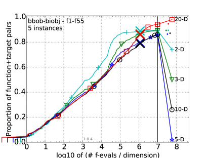
Results of HMO-CMA-ES from experiments according to [3] on the benchmark functions given in [9] are presented in Figures 1, 2, 3, 4, and 5, and in Table 1.
For each problem instance, the performance of HMO-CMA-ES is assessed in
terms of the hypervolume metric [10] (to be maximized),
the Lebesgue measure of the points that are a) dominated by at least one
objective vector found by the algorithm, and b) dominate a given
reference point. This hypervolume is assessed relative to a reference
value, which is the dominated hypervolume of a reference Pareto front
consisting of the best known set of objective vectors for this problem.
The task of maximizing the hypervolume is equivalent to minimizing the
difference between reference hypervolume and achieved hypervolume (to be
minimized). The reference hypervolume defines target values for this
difference, which are multiples of the reference hypervolume with the
factors
.
All results are reported in terms of the fraction of reached target
values. This normalization makes the results roughly comparable across
different problem types.
Hence, if an algorithm finds a non-dominated front of exactly the same quality as the best known, then it reaches 52 out of 58 targets (including ). This corresponds to roughly on the vertical axis of the plots used in this paper, i.e., a curve stopping at around suggest that the best known approximation was reached. In most cases, the best known approximation provided by the biobj-BBOB 2016 is very close to the true best value of the Pareto front and thus is about the maximum possible value one can reach. This is often the case on uni-modal functions. However, on some multi-modal functions (i.e., when at least one of the objectives is multi-modal) the current best approximation can be further improved and thus an algorithm can reach targets with negative factors corresponding to better hypervolume values than the reference of biobj-BBOB 2016. Indeed, the introduction of negative targets was motivated by the fact that the current known approximations are not the best possible ones in some cases.
Figure 1 shows the aggregated results over all 55 functions for search space dimension . The saturation at a value of can be well observed on 2-dimensional problems, where the best known hypervolume values are indeed very close to the optimal ones. In this case, HMO-CMA-ES solves most of the problems after about function evaluations, from where on the curves stagnate. The problems become harder with , hence more function evaluations are typically needed to reach a similar average performance.
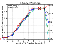
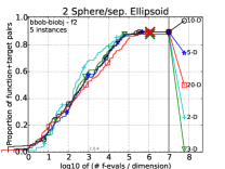
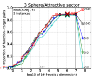
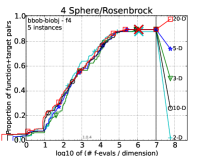
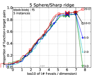
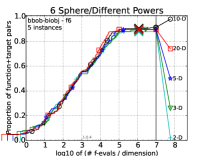
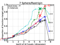
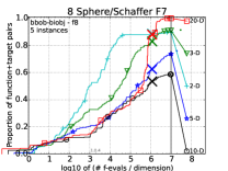
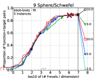
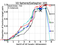
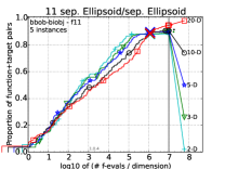
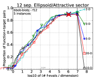
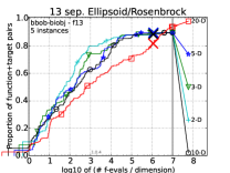
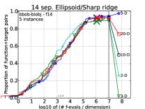
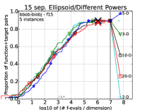
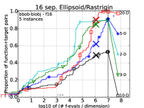
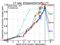
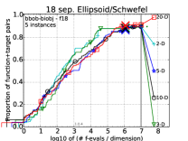
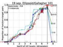
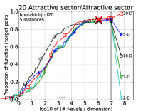
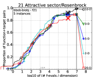
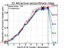
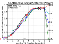
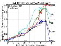
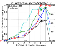
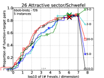
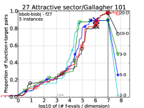
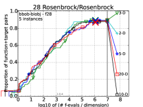
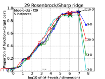
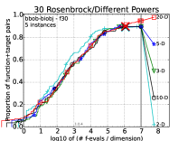
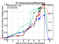
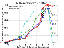
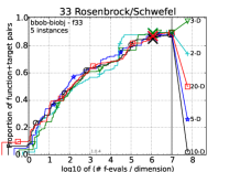
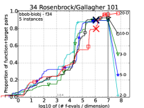
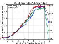
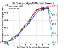
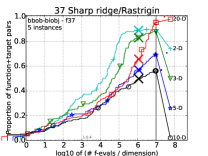
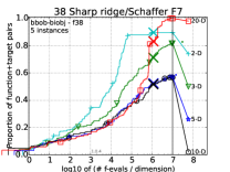
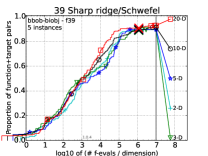
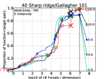
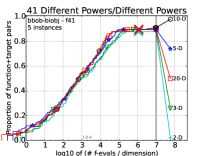
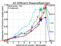
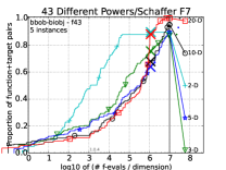
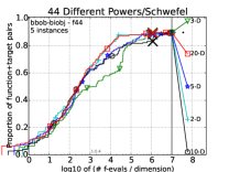
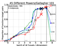
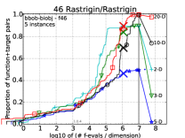
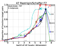
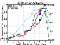
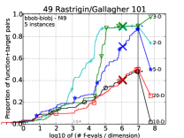
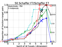
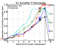
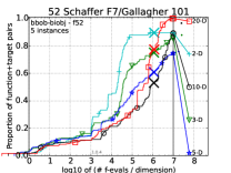
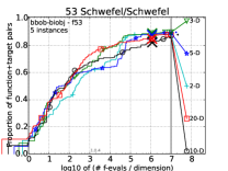
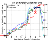
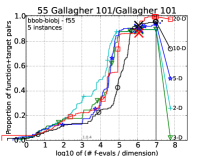
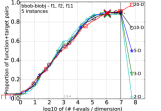
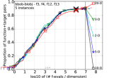
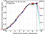
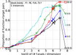
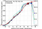
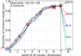
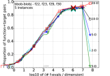
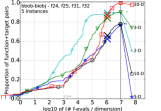
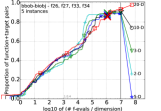
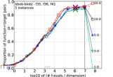
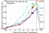
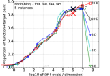
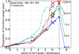
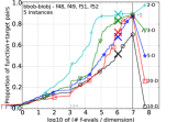
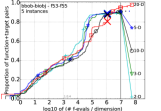
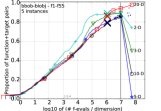
Table 1 shows the average runtime to reach given targets on 5- and 20-dimensional problems. Figures 2, 3, 4 show the empirical cumulative distribution of simulated (bootstrapped) runtimes [3] for all 55 functions and all considered problem dimensions. Some functions can be associated with a much higher variance in the results and with a faster than linear growth of the complexity w.r.t. . This is often the case for multi-modal functions, but sometimes also appears for ill-conditioned problems. On some (often 20-dimensional) problems the best known hypervolume value can be improved, this happens when the curve crosses the value of about .
5 Conclusion
We have presented a hybrid algorithm for multi-objective optimization, combining of a number of well-performing components for single- and multi-objective optimization. We showed that the proposed algorithm can solve almost all biobj-BBOB problems. When large computational budgets are considered it finds high quality solution sets for nearly all combinations of problem type and search space dimension. We attribute this robustness to the combination of different optimizer components into a hybrid algorithm. The performance relative to other multi-objective algorithms will be known as soon as the results of the biobj-BBOB 2016 edition are available.
The algorithm has a set of hyperparameters, mostly start and stop times (iteration numbers) encoded as multiples of . Better tuning of these would most probably improve its performance. It may be possible to replace some of the hard numbers with adaptive stopping criteria.
The algorithm can be outperformed on some functions even by its own individual components (the price of hybridization) or when a particular computational budget is considered (the price for its good anytime performance). It should be possible to considerably reduce these effects with online prioritization of individual components depending on their relative performance. However, this step is left for future work.
6 Acknowledgements
We thank Frank Hutter and Martin Pilát for valuable discissions.
 |
 |
 |
 |
 |
 |
 |
 |
 |
 |
 |
 |
 |
 |
 |
 |
 |
 |
 |
 |
 |
 |
 |
 |
 |
 |
 |
 |
 |
 |
 |
 |
 |
 |
 |
 |
 |
 |
 |
 |
 |
 |
 |
 |
 |
 |
 |
 |
 |
 |
 |
 |
 |
 |
 |
| separable-separable | separable-moderate | separable-ill-cond. | separable-multimodal |
 |
 |
 |
 |
| separable-weakstructure | moderate-moderate | moderate-ill-cond. | moderate-multimodal |
 |
 |
 |
 |
| moderate-weakstructure | ill-cond.-ill-cond. | ill-cond.-multimodal | ill-cond.-weakstructure |
 |
 |
 |
 |
| multimodal-multimodal | multimodal-weakstructure | weakstructure-weakstructure | all 55 functions |
 |
 |
 |
 |
5-D
1e+0
1e-1
1e-2
1e-3
1e-4
1e-5
#succ
1
76
622
3680
38122
6.1e5
5
/5
3
.0
137
675
3282
37044
3.0e5
5
/5
1
92
706
5848
44638
3.0e5
5
/5
1
105
573
2722
30360
3.0e5
5
/5
1
107
1246
26575
1.2e5
6.8e5
5
/5
1
55
698
3951
47723
2.9e5
5
/5
1
698
1.1e5
4.9e6
5.8e6
0
/5
2
.8
2622
1.7e5
2.0e6
2.7e7
5.8e6
0
/5
1
104
525
2004
20926
4.4e5
5
/5
1
390
46136
1.2e5
1.6e5
4.1e5
5
/5
1
56
519
9095
1.3e5
9.7e5
5
/5
1
53
584
6412
28731
1.6e5
5
/5
2
.0
26
300
3749
26314
86884
5
/5
1
283
2094
15271
1.3e5
3.9e5
5
/5
4
.8
101
874
6392
51584
3.1e5
5
/5
1
3283
98937
5.1e6
2.6e7
2.6e7
1
/5
48
8237
1.1e5
3.0e6
2.5e7
2.7e7
1
/5
1
62
881
7694
1.2e5
2.0e6
4
/5
4
.8
1449
51687
1.5e5
2.7e5
1.9e6
4
/5
2
.0
43
587
5553
33785
2.4e5
5
/5
1
149
13829
34787
60168
2.2e5
5
/5
1
95
1275
9521
75476
3.9e5
5
/5
1
61
662
3948
38675
2.8e5
5
/5
2
.2
536
1.3e5
3.4e6
5.8e6
0
/5
2
.4
10730
1.3e5
2.2e6
1.2e7
2.6e7
1
/5
2
.4
102
537
1672
3.8e5
4.1e6
3
/5
1
2443
83976
1.9e5
3.2e5
7.4e5
5
/5
1
24
152
1177
90425
1.5e6
5
/5
1
84
1774
16753
1.3e5
4.3e5
5
/5
1
34
476
2851
86136
4.0e5
5
/5
1
1371
67643
3.0e6
2.8e7
5.9e6
0
/5
2
.4
5032
93375
2.0e6
1.3e7
2.9e7
1
/5
2
.0
11
70
491
3.6e5
5.2e6
3
/5
1
222
43144
2.5e5
2.9e5
8.2e5
5
/5
1
102
2666
55515
3.5e5
1.5e6
5
/5
1
279
7123
40761
1.3e5
4.8e5
5
/5
1
932
1.7e5
3.3e6
2.7e7
5.9e6
0
/5
1
27778
3.1e5
1.2e7
5.9e6
0
/5
1
213
1043
89093
2.6e5
7.0e5
5
/5
1
1505
18105
1.8e5
3.7e5
1.6e6
5
/5
1
38
633
5997
42241
2.6e5
5
/5
1
648
2.4e5
4.8e6
5.9e6
0
/5
1
.8
25272
2.0e5
4.9e6
2.6e7
2.7e7
1
/5
1
51
540
1733
36645
9.6e5
5
/5
1
256
56060
1.3e5
1.8e5
4.3e5
5
/5
1
14236
4.7e5
6.0e6
0
/5
1
14416
2.7e5
6.4e6
2.7e7
2.8e7
1
/5
1
11373
95569
1.0e6
9.7e6
1.1e7
2
/5
1
2650
1.8e5
5.9e5
1.2e7
2.7e7
1
/5
1
11162
1.6e5
2.9e6
5.9e6
0
/5
1
7873
1.6e5
4.8e6
2.7e7
2.7e7
1
/5
1
10582
1.5e5
3.6e6
1.3e7
5.8e6
0
/5
2
.4
16
50
38574
88948
2.3e6
4
/5
1
89
44791
1.3e5
1.5e5
2.6e5
5
/5
1
.2
16706
1.3e5
1.7e5
2.4e5
3.1e5
5
/5
20-D
1e+0
1e-1
1e-2
1e-3
1e-4
1e-5
#succ
1
173
1414
8267
76089
3.9e5
5
/5
1
176
2284
23672
2.7e5
3.1e6
5
/5
1
271
2628
11178
88645
4.6e5
5
/5
1
175
1537
9688
92783
9.8e5
5
/5
1
229
2991
30127
1.9e5
8.0e5
5
/5
1
288
2139
13912
1.2e5
5.6e5
5
/5
1
15922
4.7e5
1.5e7
3.3e7
1.1e8
1
/5
1
40384
1.4e6
1.4e7
1.9e7
1.9e7
4
/5
1
163
1720
6034
47190
5.7e5
5
/5
1
634
2.3e5
7.3e5
9.3e5
1.3e6
5
/5
1
258
3511
1.1e5
3.2e6
1.8e7
4
/5
1
139
1524
11420
1.4e5
1.9e6
5
/5
1
175
1419
23144
9.8e6
4.6e7
2
/5
1
229
6010
53814
4.7e5
2.2e6
5
/5
1
173
1775
13552
2.3e5
1.0e7
4
/5
1
31269
5.4e5
5.1e6
1.4e7
1.4e7
4
/5
1
48714
6.0e5
4.9e6
1.5e7
1.6e7
4
/5
1
164
1567
17826
5.3e5
4.4e6
5
/5
1
6392
2.5e6
7.4e6
8.2e6
1.1e7
4
/5
1
145
2113
9529
40822
4.8e5
5
/5
1
339
1886
9899
6.0e6
6.9e6
4
/5
1
236
3727
16569
1.5e5
5.9e5
5
/5
1
236
2311
13117
94667
6.2e5
5
/5
1
15684
6.6e5
7.7e6
2.7e7
4.3e7
2
/5
1
49579
6.9e5
7.1e6
1.0e7
1.1e7
5
/5
1
107
766
2602
1.9e5
8.0e6
4
/5
1
2.1e5
1.5e6
5.4e6
7.3e6
8.0e6
4
/5
1
56
353
7009
2.9e5
1.0e7
4
/5
1
407
4107
28043
2.1e5
1.4e6
5
/5
1
117
1880
11138
1.7e5
8.2e6
4
/5
1
28458
4.6e5
1.8e7
2.5e7
4.0e7
2
/5
1
32778
4.7e5
6.7e6
1.6e7
2.1e7
4
/5
1
29
212
3520
5.7e5
1.7e7
4
/5
1
540
7.5e6
9.3e6
9.6e6
2.1e7
3
/5
1
410
4748
41160
2.4e5
7.7e5
5
/5
1
569
4542
34402
2.8e5
1.5e6
5
/5
1
7210
4.7e5
1.1e7
1.0e8
1.0e8
1
/5
1
84291
1.5e6
1.1e7
2.7e7
2.7e7
3
/5
1
488
4413
27408
1.6e5
9.1e5
5
/5
1
42097
6.4e6
1.7e7
1.7e7
1.7e7
3
/5
1
285
2579
16752
1.2e5
6.3e5
5
/5
1
48328
2.9e6
4.3e7
4.6e7
4.6e7
2
/5
1
96614
2.0e6
1.2e7
2.2e7
2.3e7
4
/5
1
171
1490
6162
40596
7.4e5
5
/5
1
54016
1.4e6
1.0e7
2.1e7
2.1e7
3
/5
1
48335
7.4e5
1.2e7
1.7e7
1.9e7
4
/5
1
60949
1.1e6
7.2e6
8.7e6
9.2e6
5
/5
1
37048
3.8e5
6.9e6
2.4e7
2.5e7
3
/5
1
2.5e5
1.9e7
2.3e7
0
/5
1
71298
6.3e5
5.0e6
7.3e6
7.4e6
5
/5
1
46809
7.1e5
6.4e6
1.5e7
1.6e7
4
/5
1
87993
4.4e6
2.6e7
2.7e7
2.7e7
3
/5
1
29
160
1905
17127
1.9e7
3
/5
1
5005
7.4e5
1.5e7
2.2e7
4.2e7
2
/5
1
2.3e5
6.4e6
7.0e6
7.1e6
7.1e6
4
/5
References
- [1] T. Glasmachers, B. Naujoks, and G. Rudolph. Start Small, Grow Big? Saving Multi-objective Function Evaluations. In Parallel Problem Solving from Nature–PPSN XIII, pages 579–588. Springer, 2014.
- [2] N. Hansen. Benchmarking a BI-population CMA-ES on the BBOB-2009 function testbed. In Proceedings of the 11th Annual Conference Companion on Genetic and Evolutionary Computation Conference: Late Breaking Papers, pages 2389–2396. ACM, 2009.
- [3] N. Hansen, T. Tusar, O. Mersmann, A. Auger, and D. Brockhoff. COCO: The Experimental Procedure. Technical Report arXiv:1603.08776, arxig.org, 2016.
- [4] C. Igel, N. Hansen, and S. Roth. Covariance matrix adaptation for multi-objective optimization. Evolutionary computation, 15(1):1–28, 2007.
- [5] C. Igel, T. Suttorp, and N. Hansen. Steady-state selection and efficient covariance matrix update in the multi-objective CMA-ES. In Evolutionary Multi-Criterion Optimization, pages 171–185. Springer, 2007.
- [6] I. Loshchilov and M. Pilát. Personal communication, 2013.
- [7] I. Loshchilov, M. Schoenauer, and M. Sebag. Bi-population CMA-ES algorithms with surrogate models and line searches. In Proceedings of the 15th annual conference companion on Genetic and evolutionary computation, pages 1177–1184. ACM, 2013.
- [8] M. J. Powell. The BOBYQA algorithm for bound constrained optimization without derivatives. 2009.
- [9] T. Tusar, D. Brockhoff, N. Hansen, and A. Auger. COCO: The Bi-objective Black Box Optimization Benchmarking (bbob-biobj) Test Suite. Technical Report arXiv:1604.00359, arxig.org, 2016.
- [10] T. Wagner, N. Beume, and B. Naujoks. Pareto-, aggregation-, and indicator-based methods in many-objective optimization. In Evolutionary multi-criterion optimization, pages 742–756. Springer, 2007.