Unconstrained Still/Video-Based Face Verification with Deep Convolutional Neural Networks

Abstract

Over the last five years, methods based on Deep Convolutional Neural Networks (DCNNs) have shown impressive performance improvements for object detection and recognition problems. This has been made possible due to the availability of large annotated datasets, a better understanding of the non-linear mapping between input images and class labels as well as the affordability of GPUs. In this paper, we present the design details of a deep learning system for unconstrained face recognition, including modules for face detection, association, alignment and face verification. The quantitative performance evaluation is conducted using the IARPA Janus Benchmark A (IJB-A), the JANUS Challenge Set 2 (JANUS CS2), and the LFW dataset. The IJB-A dataset includes real-world unconstrained faces of 500 subjects with significant pose and illumination variations which are much harder than the Labeled Faces in the Wild (LFW) and Youtube Face (YTF) datasets. JANUS CS2 is the extended version of IJB-A which contains not only all the images/frames of IJB-A but also includes the original videos. Some open issues regarding DCNNs for face verification problems are then discussed.

1 Introduction

Face verification is a challenging problem in computer vision and has been actively researched for over two decades zhao_face_2003 . In face verification, given two videos or images, the objective is to determine whether they belong to the same person. Many algorithms have been shown to work well on images and videos that are collected in controlled settings. However, the performance of these algorithms often degrades significantly on images that have large variations in pose, illumination, expression, aging, and occlusion. In addition, for an automated face verification system to be effective, it also needs to handle errors that are introduced by algorithms for automatic face detection, face association, and facial landmark detection.

Existing methods have focused on learning robust and discriminative representations from face images and videos. One approach is to extract an over-complete and high-dimensional feature representation followed by a learned metric to project the feature vector onto a low-dimensional space and then compute the similarity scores. For example, high-dimensional multi-scale local binary pattern (LBP) chen_blessing_2012 features extracted from local patches around facial landmarks and Fisher vector (FV) simonyan_fisher_2013 ; Chan_FV_BTAS_2015 features have been shown to be effective for face recognition. Despite significant progress, the performance of these systems has not been adequate for deployment. However, given the availability of millions of annotated data, faster GPUs and a better understanding of the nonlinearities, DCNNs are providing much better performance on tasks such as object recognition krizhevsky_imagenet_2012 ; szegedy_going_2014 , object/face detection girshick_rich_2014 ; ranjan_deep_2015 , face verification/recognition schroff_facenet_2015 ; parkhi_deep_2015 . It has been shown that DCNN models can not only characterize large data variations but also learn a compact and discriminative representation when the size of training data is sufficiently large. In addition, it can be generalized to other vision tasks by fine-tuning the pre-trained model on the new task donahue_decaf_2013 .

In this paper, we present an automated face verification system. Due to the robustness of DCNNs, we build each component of our system based on separate DCNN models. Modules for detection and face alignment use the DCNN architecture proposed in krizhevsky_imagenet_2012 . For face verification, we train two DCNN models trained using the CASIA-WebFace yi_learning_2014 dataset. Finally, we compare the performance of our approach with many face matchers on the IJB-A dataset which are being carried out or have been recently reported nist_ijba_2016 The proposed system is fully automatic. Although the IJB-A dataset contains significant variations in pose, illumination, expression, resolution and occlusion which are much harder than the Labeled Faces in the Wild (LFW) datasets, we present verification results for the LFW dataset too.
The system described in this paper, which integrates DCNN-based face detection ranjan_deep_2015 and fiducial point detection kumar_face_2016 modules differs from its predecessor chen2015end in the following ways: (1) uses more robust features from two networks which take faces as input with different resolutions (Section 3.4) are used and (2) employs a more efficient metric learning method tse which uses inner-products based constraints between triplets to optimize for the embedding matrix as opposed to norm-based constraints used in other methods (Section 3.5). In the experimental section, we also demonstrate the improvement due to media-sensitive pooling and the fusion of two networks.

The rest of the paper is organized as follows. We briefly review closely related works in Section 2. In Section 3, we present the design details of a deep learning system for unconstrained face verification and recognition, including face detection, face association, face alignment, and face verification. Experimental results using IJB-A, CS2, and LFW datasets are presented in Section 4. Some open issues regarding the use of DCNNs for face recognition/verification problems are discussed in Section 5. Finally, we conclude the paper in Section 6 with a brief summary and discussion.

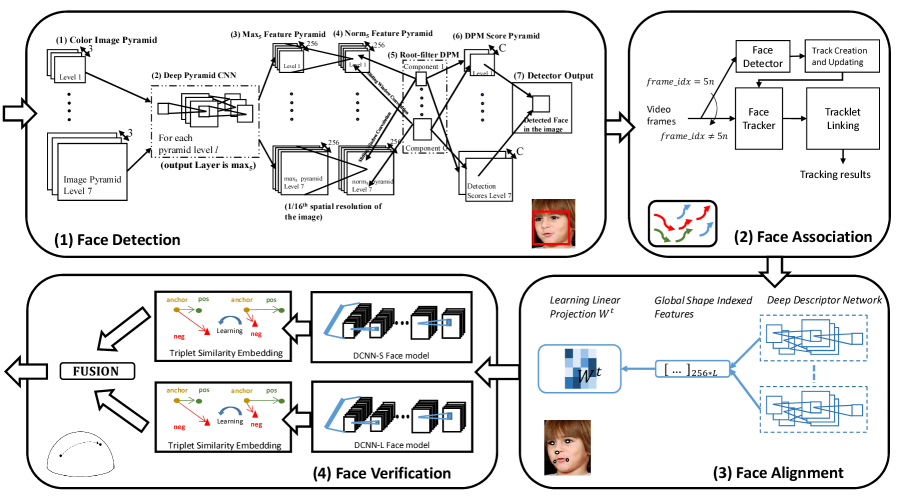
Figure 1: An overview of the proposed DCNN-based face verification system.

2 Related Work

A typical face verification system consists of the following components: (1) face detection and (2) face association across video frames, (3) facial landmark detection to align faces, and (4) face verification to verify a subject’s identity. Due to the large number of published papers in the literature, we briefly review some relevant works for each component.

2.1 Face Detection

The face detection method introduced by Viola and Jones viola_robust_2004 is based on cascaded classifiers built using Haar wavelet features. Since then, a variety of sophisticated cascade-based face detectors such as Joint Cascade JointCascade_LI_ECCV2014 , SURF Cascade 6619289 and CascadeCNN CascadeCNN_CVPR2015 have demonstrated improved performance. Zhu et al. zhu2012face improved the performance of face detection algorithm using the deformable part model (DPM) approach, which treats each facial landmark as a part and uses HOG features to simultaneously perform face detection, pose estimation, and landmark localization. A recent face detector, Headhunter HeadHunter_Mathias_ECCV2014 , demonstrated competitive performance using a simple DPM. However, the key challenge in unconstrained face detection is that features like Haar wavelets and HOG do not capture the salient facial information at different poses and illumination conditions. To overcome these limitations, several deep CNN-based face detection methods have been proposed in the literature such as Faceness faceness_ICCV2015 , DDFD DDFD_ICMR2015 and CascadeCNN CascadeCNN_CVPR2015 . It has been shown in donahue_decaf_2013 that a deep CNN pre-trained with the Imagenet dataset can be used as a meaningful feature extractor for various vision tasks. The method based on Regions with CNN (R-CNN) girshick_fastrcnn_15 computes region-based deep features and attains state-of-art face detection performance. In addition, since the deep pyramid girshick_deformable_2014 removes the fixed-scale input dependency in deep CNNs, it is attractive to be integrated with the DPM approach to further improve the detection accuracy across scale ranjan_deep_2015 .

2.2 Face Association

Video-based face verification systems Chen2012_MOT requires consistently-tracked faces to capture diverse pose and spatial-temporal information for analysis. In addition, there is usually more than one person present in the videos, and thus multiple face images from different individuals should be correctly associated across the video frames. Several recent techniques have tracked multiple objects by modeling the motion context Yoon2015MOT , track management Duffner2013MOT , and guided tracking using the confidence map of the detector Breitenstein2009MOT . Multi-object tracking methods based on tracklet linking Huang2008MOT ; Roth2012 ; Bae2014 usually rely on the Hungarian algorithm Ahuja1993 to optimally assign the detected bounding boxes to existing tracklets. Roth et al. Roth2012 adapted the framework of multi-object tracking methods based on tracklet linking approach to track multiple faces; Several face-specific metrics and constraints have been introduced to enhance the reliability of face tracker. A recent study Comaschi2015MOT proposed to manage the tracks generated by a continuous face detector without relying on long-term observations. In unconstrained scenarios, the camera can undergo abrupt movements, which makes persistent tracking a challenging task. Du et al. proposed a conditional random field (CRF) framework for face association in two consecutive frames by utilizing the affinity of facial features, location, motion, and clothing appearance Du2012 . Our face association method utilizes the KLT tracker to track a face initiated from the face detection. We continuously update the face tracking results for every fifth frame using the detected faces. The tracklet linking Bae2014 is utilized to link the fragmented tracklet. We present a robust face association method based on existing works in Everingham2009MOT ; Bae2014 ; Shi1994 . In addition, recently developed object trackers babenko2009visual ; henriques2015high ; kalal2012tracking and face trackers wang2008robust ; lui2010adaptive can be integrated to potentially improve the robustness of face association method. More details are presented in Section 3.2.

2.3 Facial Landmark Detection

Facial landmark detection is an important component to align the faces into canonical coordinates and to improve the performance of verification algorithms. Pioneering works such as Active Appearance Models (AAM) cootes_active_2001 and Active Shape Models (ASM) cootes_active_1995 are built using the PCA constraints on appearance and shape. In cristinacce_feature_2006 , Cristinacce et al. generalized the ASM model to a Constrained Local Model (CLM), in which every landmark has a shape constrained descriptor to capture the appearance. Zhu et al. zhu2012face used a part-based model for face detection, pose estimation and landmark localization assuming the face shape to be a tree structure. Asthana et al. asthana_robust_2013 combined the discriminative response map fitting with CLM. In addition, Cao et. al. cao2014face followed the cascaded pose regression (CPR) proposed by $Doll\acute{a}r$ et. al. dollar2010cascaded : feature extraction followed by a regression stage. However, unlike CPR which uses pixel difference as features, it trains a random forest based on local binary patterns. In general, these methods learn a model that directly maps the image appearance to the target output. Nevertheless, the performance of these methods depends on the robustness of local descriptors. In krizhevsky_imagenet_2012 , the deep features are shown to be robust to different challenging variations. Sun et al. sun_deep_2013 proposed a cascade of carefully designed CNNs, in which at each level, outputs of multiple networks are fused for landmark estimation and achieve good performance. Unlike sun_deep_2013 , we use a single CNN, carefully designed to provide a unique key-point descriptor and achieve better performance. Besides using a 2D transformation for face alignment, Hassner et al. hassner2015effective proposed an effective method to frontalize faces with the help of generic 3D face model. However, the effectiveness of the method also highly relies on the quality of the detected facial landmarks (i.e., the method usually introduces undesirable artifacts when the quality of facial landmarks is poor).

2.4 Feature Representation for Face Recognition

Learning invariant and discriminative feature representations is a critical step in designing a face verification system. Ahonen et al. ahonen_face_2006 showed that the Local Binary Pattern (LBP) is effective for face recognition. Chen et al. chen_blessing_2012 demonstrated good results for face verification using high-dimensional multi-scale LBP features extracted from patches extracted around facial landmarks. However, recent advances in deep learning methods have shown that compact and discriminative representations can be learned using a DCNN trained with very large datasets. Taigman et al. taigman_deepface_2014 built a DCNN model on the frontalized faces generated with a general 3D shape model from a large-scale face dataset and achieved better performance than many traditional methods. Sun et al. sun_deeply_2014 achieved results that surpass human performance for face verification on the LFW dataset using an ensemble of 25 simple DCNN with fewer layers trained on weakly aligned face images from a much smaller dataset than taigman_deepface_2014 . Schroff et al. schroff_facenet_2015 adapted a state-of-the-art object recognition network to face recognition and trained it using a large-scale unaligned private face dataset with triplet loss. Parkhi et al. parkhi_deep_2015 trained a very deep convolutional network based on VGGNet for face verification and demonstrated impressive results. These studies essentially demonstrate the effectiveness of the DCNN model for feature learning and detection/recognition/verification problems.

2.5 Metric Learning

Learning a similarity measure from data is the other key component for improving the performance of a face verification system. Many approaches have been proposed in the literature that essentially exploit label information from face images or face pairs. For instance, Weinberger et al. weinberger_distance_2005 used the Large Margin Nearest Neighbor (LMNN) metric which enforces the large margin constraint among all triplets of labeled training data. Guillaumin et al. guillaumin2009you proposed two robust distance measures: Logistic Discriminant-based Metric Learning (LDML) and Marginalized kNN (MkNN). The LDML method learns a distance by performing a logistic discriminant analysis on a set of labeled image pairs and the MkNN method marginalizes a k-nearest-neighbor classifier to both images of the given test pair using a set of labeled training images. Mignon et al. mignon2012pcca proposed an algorithm for learning distance metrics from sparse pairwise similarity/dissimilarity constraints in high dimensional input space. The method exhibits good generalization properties when projecting the features from a high-dimensional space to a low-dimensional one. Nguyen et al. nguyen2010cosine used an efficient and simple metric learning method based on the cosine similarity measure instead of the widely adopted Euclidean distance. Taigman et al. taigman_multiple_2009 employed the Mahalanobis distance using the Information Theoretic Metric Learning (ITML) method davis_information_2007 . Chen et al. chen_bayesian_2012 used a joint Bayesian approach for face verification which models the joint distribution of a pair of face images and uses the ratio of between-class and within-class probabilities as the similarity measure. Hu et al. hu_discriminative_2014 learned a discriminative metric within the deep neural network framework. Schroff et al. schroff_facenet_2015 and Parkhi et al. parkhi_deep_2015 optimized the DCNN parameters based on the triplet loss which directly embeds the DCNN features into a discriminative subspace and presented promising results for face verification.

3 Proposed System

The proposed system is a complete pipeline for performing automatic face verification. We first perform face detection to localize faces in each image and video frame. Then, we associate the detected faces with the common identity across video frames and align the faces into canonical coordinates using the detected landmarks. Finally, we perform face verification to compute the similarity between a pair of images/videos. The system is illustrated in Figure 1. The details of each component are presented in the following sections.

3.1 Face Detection

All the faces in the images/video frames are detected using a DCNN-based face detector, called the Deep Pyramid Deformable Parts Model for Face Detection (DP2MFD) ranjan_deep_2015 , which consists of two modules. The first module generates a seven level normalized deep feature pyramid for any input image of arbitrary size, as illustrated in the first part of Figure 1. The architecture of Alexnet krizhevsky_imagenet_2012 is adopted for extracting the deep features. This image pyramid network generates a pyramid of 256 feature maps at the fifth convolution layer (conv₅). A 3 $\times$ 3 max filter is applied to the feature pyramid at a stride of one to obtain the max₅ layer. Typically, the activation magnitude for a face region decreases with the size of the pyramid level. As a result, a large face detected by a fixed-size sliding window at a lower pyramid level will have a high detection score compared to a small face getting detected at a higher pyramid level. In order to reduce this bias to face size, we apply a z-score normalization step on the max₅ features at each level. For a 256-dimensional feature vector $x_{i,j,k}$ at the pyramid level i and location $(j,k)$, the normalized feature $x_{i,j,k}$ is computed as:

$$x_{i,j,k}=\frac{x_{i,j,k}-\mu_{i}}{\sigma_{i}},$$ (1)

where $\mu_{i}$ is the mean feature vector, and $\sigma_{i}$ is the standard deviation for the pyramid level i. We refer to the normalized max₅ features as $norm_{5}$. Then, the fixed-length features from each location in the pyramid are extracted using the sliding window approach.

The second module is a linear SVM, which takes these features as inputs to classify each location as face or non-face, based on their scores. A root-only DPM is trained on the norm₅ feature pyramid using a linear SVM. In addition, the deep pyramid features are robust to not only pose and illumination variations but also to different scales. The DP2MFD algorithm works well in unconstrained settings as shown in Figure 2. We also present the face detection performance results under the face detection protocol of the IJB-A dataset in Section  4.

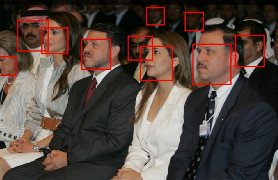
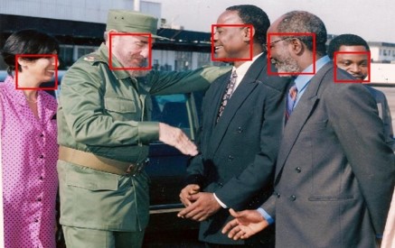
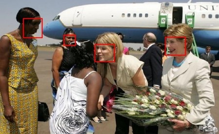
Figure 2: Sample detection results on an IJB-A image using the deep pyramid method.

3.2 Face Association

Because there are multiple subjects appearing in the frames of each video of the IJB-A dataset, performing face association to assign each face to its corresponding subject is an important step to pick the correct subject for face verification. Thus, once the faces in the images and video frames are detected, we track multiple faces by integrating results from the face detector, face tracker, and a tracklet linking step. The second part of Figure 1 shows the block diagram of the multiple face tracking system. We apply the face detection algorithm in every fifth frame using the face detection method presented in Section 3.1. The detected bounding box is considered as a novel detection if it does not have an overlap ratio with any bounding box in the previous frames larger than $\gamma$. The overlap ratio of a detected bounding box $\mathbf{b}_{d}$ and a bounding box $\mathbf{b}_{tr}$ in the previous frames is defined as

$$s(\mathbf{b}_{d},\mathbf{b}_{tr})=\frac{area(\mathbf{b}_{d}\cap\mathbf{b}_{tr})}{area(\mathbf{b}_{tr})}.$$ (2)

We empirically set the overlap threshold $\gamma$ to $0.2$. A face tracker is created from a detection bounding box that is treated as a novel detection. We set the face detection confidence threshold to -1.0 to select bounding boxes of face detection of high confidence. For face tracking, we use the Kanade-Lucas-Tomasi (KLT) feature tracker Shi1994 to track the faces between two consecutive frames. To avoid the potential drift of trackers, we update the bounding boxes of the tracker by those provided by the face detector in every fifth frame. The detection bounding box $\mathbf{b}_{d}$ replaces the tracking bounding boxes $\mathbf{b}_{tr}$ of a tracklet in the previous frame if $s(\mathbf{b}_{d},\mathbf{b}_{tr})\leq\gamma$. A face tracker is terminated if there is no corresponding face detection overlapping with it for more than $t$ frames. We set $t$ to 4 based on empirical grounds.
In order to handle the fragmented face tracks resulting from occlusions or unreliable face detection, we use the tracklet linking method proposed by Bae2014 to associate the bounding boxes in the current frames with tracklets in the previous frames. The tracklet linking method consists of two stages. The first stage is to associate the bounding boxes provided by the tracker or the detector in the current frame with the existing tracklet in previous frames. This stage consists of local and global associations. The local association step associates the bounding boxes with the set of tracklets, having high confidence. The global step associates the remaining bounding boxes with the set of tracklets of low confidence. The second stage is to update the confidence of the tracklets, which will be used for determining the tracklets for local or global association in the first stage. We show sample face association results for some videos from the CS2 dataset in Figure 3.

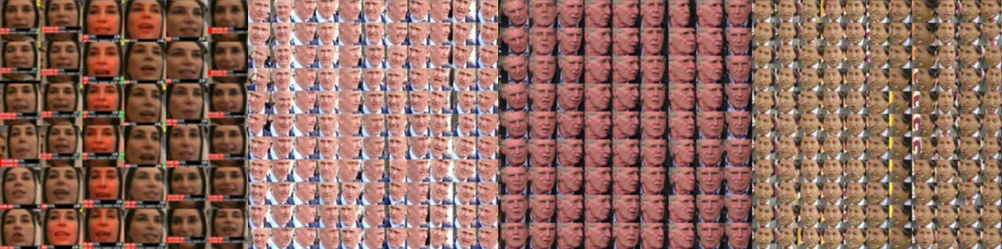
Figure 3: Sample results of our face association method for videos of JANUS CS2 which is the extension dataset of IJB-A.

3.3 Facial Landmark Detection

Once the faces are detected or associated, we perform facial landmark detection for face alignment. The DCNN-based facial landmark detection algorithm module, local deep descriptor regression (LDDR) kumar_face_2016 , works in two stages. We model the task as a regression problem, where beginning with the initial mean shape, the target shape is reached through regression. The first step is to perform feature extraction of a patch around a point of the shape followed by linear regression as described in 6909614 ; cao2014face . Given a face image $I$ and the initial shape $S^{0}$, the regressor computes the shape increment $\Delta S$ from the deep descriptors and updates the face shape using (3).

$$S^{t}=S^{t-1}+W^{t}\Phi^{t}(I,S^{t-1})$$ (3)

The CNN features (represented as $\Phi$ in 3) carefully designed with the proper number of strides and pooling (refer to Table 1 for more details), are used as features to perform regression. We use the same CNN architecture as Alexnet krizhevsky_imagenet_2012 with the pretrained weights for the ImageNet dataset as shown in Figure 4. Then, we further fine-tuned it with AFLW tugraz:icg:lrs:koestinger11b dataset for face detection task. The fine-tuning step helps the network to learn features specific to faces. Furthermore, we adopt the cascade regression, in which the output generated by the first stage is used as an input for the next stage. The number of stages is fixed at 5 in our system. The patches selected for feature extraction are reduced subsequently in later stages to improve the localization of facial landmarks. After the facial landmark detection is completed, each face is aligned into the canonical coordinate using the similarity transform and seven landmark points (i.e., two left eye corners, two right eye corners, nose tip, and two mouth corners).

Stage 1	Input Size (pixels)	conv1	max1	conv2	max2
Stage 1	$92\times 92$	4	2	1	1
Stage 2	$68\times 68$	3	2	1	1
Stage 3	$42\times 42$	2	1	1	2
Stage 4	$21\times 21$	1	1	1	1

Table 1: Input size and the number of strides in conv1, max1, conv2 and max2 layers for 4 stages of regression kumar_face_2016 .

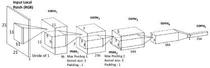
Figure 4: The DCNN architecture used to extract the local descriptors for the facial landmark detection task kumar_face_2016 .

3.4 Deep Convolutional Face Representation

In this work, we train two deep convolutional networks. One is trained using tight face bounding boxes (DCNN_S), and the other using large bounding boxes which include more contextual (DCNN${}_{L})$ information. In Section 4, we present results which show that both networks capture discriminative information and complement each other. In addition, the fusion of two networks does significantly improve the final performance. The architectures of both networks are summarized in Tables 3 and 3.

Stacking small filters to approximate large filters and building very deep convolutional networks reduces the number of parameters but also increases the nonlinearity of the network as discussed in simonyan_verydeep_2014 ; szegedy_going_2014 . In addition, the resulting feature representation is compact and discriminative. Therefore, for (DCNN_S), we use the same network architecture presented in chen_unconstrained_2015 and train it using the CASIA-WebFace dataset yi_learning_2014 . The dimensionality of the input layer is $100\times 100\times 3$ for RGB images. The network includes ten convolutional layers, five pooling layers, and one fully connected layer. Each convolutional layer is followed by a parametric rectified linear unit (PReLU) he_delving_2015 , except the last one, conv52. Moreover, two local normalization layers are added after conv12 and conv22, respectively, to mitigate the effect of illumination variations. The kernel size of all filters is $3\times 3$. The first four pooling layers use the max operator, and pool₅ uses average pooling. The feature dimensionality of pool₅ is thus equal to the number of channels of conv52 which is 320. The dropout ratio is set as 0.4 to regularize Fc6 due to the large number of parameters (i.e. 320 $\times$ 10548 .). The pool₅ feature is used for face representation. The extracted features are further $L_{2}$-normalized to unit length before the metric learning stage. If there are multiple images and frames available for the subject template, we use the average of pool₅ features as the overall feature representation.

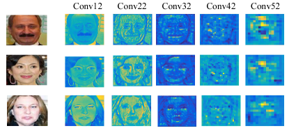
Figure 5: An illustration of some feature maps of conv12, conv22, conv32, conv42, and conv52 layers of DCNN_S trained for the face identification task. At upper layers, the feature maps capture more global shape features which are also more robust to illumination changes than conv12. The feature maps are rescaled to the same size for visualization purpose. The green pixels represent high activation values, and the blue pixels represent low activation values as compared to the green.

Name	Type	Filter Size/Stride	$\#$Params
conv11	convolution	3$\times$3 / 1	0.84K
conv12	convolution	3$\times$3 / 1	18K
pool1	max pooling	2$\times$2 / 2
conv21	convolution	3$\times$3 / 1	36K
conv22	convolution	3$\times$3 / 1	72K
pool2	max pooling	2$\times$2 / 2
conv31	convolution	3$\times$3 / 1	108K
conv32	convolution	3$\times$3 / 1	162K
pool3	max pooling	2$\times$2 / 2
conv41	convolution	3$\times$3 / 1	216K
conv42	convolution	3$\times$3 / 1	288K
pool4	max pooling	2$\times$2 / 2
conv51	convolution	3$\times$3 / 1	360K
conv52	convolution	3$\times$3 / 1	450K
pool5	avg pooling	7$\times$7 / 1
dropout	dropout (40%)
fc6	fully connected	10548	3296K
loss	softmax	10548
total			5M

Table 2: The architectures of DCNN_S.

Name	Type	Filter Size/Stride	$\#$Params
conv1	convolution	11$\times$11 / 4	35K
pool1	max pooling	3$\times$3 / 2
conv2	convolution	5$\times$5 / 2	614K
pool2	max pooling	3$\times$3 / 2
conv3	convolution	3$\times$3 / 2	885K
conv4	convolution	3$\times$3 / 2	1.3M
conv5	convolution	3$\times$3 / 1	885K
conv6	convolution	3$\times$3 / 1	590K
pool6	max pooling	3$\times$3 / 2
fc6	fully connected	1024	9.4M
dropout	dropout (50%)
fc7	fully connected	512	524K
dropout	dropout (50%)
fc8	fully connected	10548	5.5M
loss	softmax	10548
total			19.8M

Table 3: The architecture of DCNN_L.

On the other hand, for DCNN_L, the deep network architecture closely follows the architecture of the AlexNet krizhevsky_imagenet_2012 with some notable differences: reduced number of parameters in the fully connected layers; use of Parametric Rectifier Linear units (PReLU’s) instead of ReLU, since they allow a negative value for the output based on a learnt threshold and have been shown to improve the convergence rate he_delving_2015 .

The reason for using the AlexNet architecure in the convolutional layers is due to the fact that we initialize the convolutional layer weights with weights from the AlexNet model which was trained using the ImageNet challenge dataset. Several recent works (transfer1 ,transfer2 ) have empirically shown that this transfer of knowledge across different networks, albeit for a different objective, improves performance and more significantly reduces the need to train using a large number of iterations. To learn more domain specific information, we add an additional convolutional layer, conv6 and initialize the fully connected layers fc6-fc8 from scratch. Since the network is used as a feature extractor, the last layer fc8 is removed during deployment, thus reducing the number of parameters to 15M. When the network is deployed. the features are extracted from fc7 layers resulting in a dimensionality of 512. The network is trained using the CASIA-WebFace dataset yi_learning_2014 . The dimensionality of the input layer is $227\times 227\times 3$ for RGB images.

In Figure 5, we show some feature activation maps of the DCNN_S model. At upper layers, the feature maps capture more global shape features which are also more robust to illumination changes than Conv12 where the green pixels represent high activation values, and the blue pixels represent low activation values compared to the green.

3.5 Triplet Similarity Embedding

To further improve the performance of our deep features, we obtain a low-dimensional discriminative projection of the deep features, called the Triplet Similarity Embedding (TSE) that is learnt using the training data provided for each split of IJB-A. The output of the procedure is an embedding matrix $\mathbf{W}\in\mathbf{R}^{n\times M}$ where $M$ is the dimensionality of the deep descriptor (320 for DCNN_S and 512 for DCNN_L) and we set $n=128$, thus achieving dimensionality reduction in addition to an improvement in performance.

In addition, for the TSE approach, the objective was two-fold (1) to achieve as small dimensionality as possible for both networks (2) to obtain a more discriminative representation in the low dimensional space which means to push similar pairs together and dissimilar pairs apart in the low-dimensional space. For learning $\mathbf{W}$, we solve an optimization problem based on constraints involving triplets - each containing two similar samples and one dissimilar sample. Consider a triplet $\{a,p,n\}$, where $a$ (anchor) and $p$ (positive) are from the same class, but $n$ (negative) belongs to a different class. Our objective is to learn a linear projection $\mathbf{W}$ from the data such that the following constraint is satisfied:

$$(\mathbf{W}a)^{T}\cdot(\mathbf{W}p)>(\mathbf{W}a)^{T}\cdot(\mathbf{W}n)$$ (4)

In our case, $\{a,p,n\}\in\mathbf{R}^{M}$ are deep descriptors which are normalized to unit length. As such, $(\mathbf{W}a)^{T}\cdot(\mathbf{W}p)$ is the dot-product or the similarity between ${a,p}$ under the projection $\mathbf{W}$. The constraint in (4) requires that the similarity between the anchor and positive samples should be higher than the similarity between the anchor and negative samples in the low dimensional space represented by $\mathbf{W}$. Thus, the mapping matrix $\mathbf{W}$ pushes similar pairs closer and dissimilar pairs apart, with respect to the anchor point. By choosing the dimensionality of $\mathbf{W}$ as $n\times M$ where $n<M$, we achieve dimensionality reduction in addition to better performance. For our work, we fix $n=128$ based on cross validation.

Given a set of labeled data points, we solve the following optimization problem:

$$\underset{\mathbf{W}}{\text{argmin}}\sum_{{a,p,n}\in\mathbb{T}}max(0,\alpha+a^{T}\mathbf{W^{T}W}n-a^{T}\mathbf{W^{T}W}p)$$ (5)

where $\mathbb{T}$ is the set of triplets and $\alpha$ is a margin parameter chosen based on the validation set. In practice, the above problem is solved in a Large-Margin framework using Stochastic Gradient Descent (SGD) and the triplets are sampled online. The update step for solving (5) with SGD is:

$$\mathbf{W}_{t+1}=\mathbf{W}_{t}-\eta*\mathbf{W}_{t}*(a(n-p)^{T}+(n-p)a^{T})$$ (6)

where $\mathbf{W}_{t}$ is the estimate at iteration $t$, $\mathbf{W}_{t+1}$ is the updated estimate, $\{a,p,n\}$ is the triplet sampled at the current iteration and $\eta$ is the learning rate which is set to 0.01 for the current work.

The entire procedure takes 3-5 minutes per split using a standard C++ implementation. More details regarding the optimization algorithm can be found in tse . At each iteration, we sample 1000 instances from the whole training set to choose the negatives. Since the training set is relatively small for the datasets considered in this experiment, the entire training set is held in memory. Going forward this could be made efficient by using a buffer which will be replenished periodically, thus requiring a constant memory requirement. The computational complexity of each iteration is $O(M^{2})$, that is, the complexity varies quadratically with the dimension of the deep descriptor. The technique closest to the one presented in this section, which is used in recent works (parkhi_deep_2015 ,schroff_facenet_2015 ) computes the embedding $\mathbf{W}$ based on satisfying the distance constraints given below:

$$\underset{\mathbf{W}}{\text{argmin}}\sum_{{a,p,n}\in\mathbb{T}}max\{0,\alpha+(a-p)^{T}\mathbf{W^{T}W}(a-p)-$$ (7)

$$(a-n)^{T}\mathbf{W^{T}W}(a-n)\}$$ (8)

To be consistent with the terminology used in this paper, we call it Triplet Distance Embedding (TDE). It should be noted that the TSE formulation is different from TDE, in that, the current work uses inner-product based constraints between triplets to optimize for the embedding matrix as opposed to norm-based constraints used in the TDE method. To choose the dimensionality, we test the values 64,128,256 using a 5 fold validation scheme for each split. The learning rate is chosen as 0.02 and is fixed throughout the procedure. The margin parameter is chosen as 0.1. We find from our experiments that the lower margin works better but since we perform hard negative mining at each step, the method is not particularly sensitive to the margin parameter.

In general, to learn a reasonable distance measure directly using pairwise or triplet metric learning approach requires huge amount of data (i.e.,, the state-of-the-art approach schroff_facenet_2015 uses 200M images). In addition, the proposed approach decouples the DCNN feature learning and metric learning steps due to memory constraints. To learn a reasonable distance measure requires generating the informative pairs or triplets. The batch size used for SGD is limited by the memory size of the graphics card. If the model is trained end-to-end, then only a small batch size is available for use. Thus, in this work, we perform DCNN model training and metric learning independently. In addition, for the publicly available deep model parkhi_deep_2015 , it is also trained first with softmax loss and followed by finetuning the model with verification loss while freezing the convolutional and fully connected layers except the last one so that the transformation which is equivalent to the proposed approach can be learned.

4 Experimental Results

In this section, we present the results of the proposed automatic system for both face detection and face verification tasks on the challenging IARPA Janus Benchmark A (IJB-A)  klare_janus_2015 , its extended version Janus Challenging set 2 (JANUS CS2) dataset, and the LFW dataset. The JANUS CS2 dataset contains not only the sampled frames and images in the IJB-A, but also the original videos. In addition, the JANUS CS2 dataset includes considerably more test data for identification and verification problems in the defined protocols than the IJB-A dataset. The receiver operating characteristic curves (ROC) and the cumulative match characteristic (CMC) scores are used to evaluate the performance of different algorithms for face verification. The ROC curve measures the performance in verification scenarios, where the vertical axis is true acceptance rate (TAR) which represents the degree to correctly match the face image (i.e., deep features) from the same person and the horizontal axis shows false acceptance rate (FAR) which represents the degree to falsely match the biometric information from one person to another. The CMC score measures the accuracy in closed set identification scenarios.

4.1 Face Detection on IJB-A

The IJB-A dataset contains images and sampled video frames from 500 subjects collected from online media klare_janus_2015 , cheney_unconstrained_2015 . For face detection task, there are 67,183 faces of which 13,741 are from images and the remaining are from videos. The locations of all faces in the IJB-A dataset have been manually annotated. The subjects were captured so that the dataset contains wide geographic distribution. Nine different face detection algorithms were evaluated on the IJB-A dataset cheney_unconstrained_2015 , and the algorithms compared in cheney_unconstrained_2015 include one commercial off the shelf (COTS) algorithm, three government off the shelf (GOTS) algorithms, two open source face detection algorithms (OpenCV’s Viola Jones and the detector provided in the Dlib library), and GOTS ver 4 and 5. In Figure 7, we show the precision-recall (PR) curves and the ROC curves, respectively corresponding to the method used in our work and one of the best reported methods in cheney_unconstrained_2015 . We see that the face detection algorithm used in our system outperforms the best performing method reported in cheney_unconstrained_2015 by a large margin. In Figure 8 (b), we illustrate typical faces in the IJB-A dataset that are not detected by DP2MFD, and we can find the faces to be usually in very extreme conditions which contain limited information for face verification. However, in Figure 8 (a), we also show that the DP2MFD algorithm can handle very difficult faces but relatively reasonable as compared to those in 8 (b). As shown in Figure 6, the DP2MFD algorithm also achieves top performance in the challenging FDDB benchmark fddbTech for face detection with a large performance margin compared to most algorithms. Some of the recent published methods compared in the FDDB evaluation include Facenessfaceness_ICCV2015 , HeadHunter HeadHunter_Mathias_ECCV2014 , JointCascade JointCascade_LI_ECCV2014 , CCF CCF_ICCV2015 , Squares- ChnFtrs-5 HeadHunter_Mathias_ECCV2014 , CascadeCNN CascadeCNN_CVPR2015 , Structured Models Yan2014790 , DDFD DDFD_ICMR2015 , NDPFace NPDFace_PAMI2015 , PEP-Adapt PEP_Adapt_LI_ICCV2013 and TSM zhu2012face . More comparison results with other face detection data sets are available in ranjan_deep_2015 . Since the CS2 dataset has not been released to public, we are not able to provide comparisons with other existing face detectors.

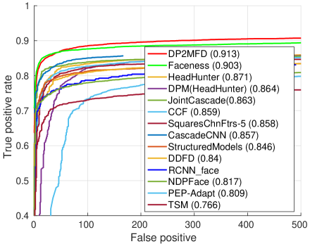
Figure 6: Face detection performance evaluation on the FDDB dataset ranjan_deep_2015 .

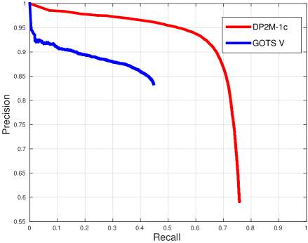
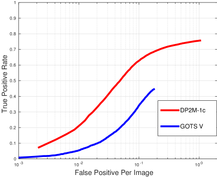
Figure 7: Face detection performance evaluation on the IJB-A dataset: (a) Precision vs. recall curves. (b) ROC curves ranjan_deep_2015 .

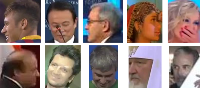
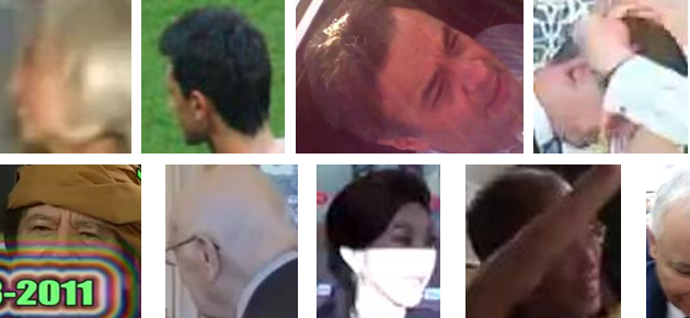
Figure 8: (a) shows the difficult faces in the IJB-A dataset that are successfully detected by DP2MFD, and (b) shows faces that are not detected by DP2MFD. From the results, we can see that DP2MFD can handle difficult occlusion, partial face, large illumination and pose variations.

4.2 Facial Landmark Detection on IJB-A

We also evaluate the performance of our facial landmark detection method on the IJB-A dataset. For the training data, we take 3148 images in total from the LFPW belhumeur2013localizing , Helen le2012interactive and AFW zhu2012face datasets and test on the IJB-A dataset. The subjects were captured so that the dataset contains wide geographic distribution. The challenge comes through the wide diversity in pose, illumination and resolution. Our method produces 68 facial landmark points following MultiPIE gross2010multi markup format. We evaluate the performance using the Normalized Mean Square Error and average pt-pt error (normalized by face size) vs fraction of images plots of different methods. Since IJB-A is annotated only with 3 key-points on the faces (two eyes and nose base) by human annotators, the interoccular distance error was normalized by the distance between nose tip and the midpoint of the eye centers. In Figure 9, we present a comparison of our algorithm with zhu2012face , asthana2013robust and kazemi2014one . For the Helen dataset, we show the performance of 49-point and full 68-point results in Table 4. Our deep descriptor-based global shape regression method outperforms the above mentioned state-of-the-art methods in both high-quality (Helen) and low-quality (IJB-A) images. Samples of detected landmarks results are shown in Figure 10. More evaluation results for landmark detection on other standard datasets may be found in kumar_face_2016 . Once facial landmark detection is completed, we choose seven landmark points (i.e. two left eye corners, two right eye corners, nose tip, and two mouth corners) out of the detected 68 points and apply the similarity transform to warp the faces into canonical coordinates.

Method	68-pts	49-pts
Zhu et al. zhu2012face	8.16	7.43
DRMF asthana2013robust	6.70	-
RCPR RCPR	5.93	4.64
SDM 6618919	5.50	4.25
GN-DPM 6909635	5.69	4.06
CFAN DBLP:conf/eccv/ZhangSKC14	5.53	-
CFSS Zhu_2015_CVPR	4.63	3.47
LDDR(Ours)	4.76	2.36

Table 4: Averaged error comparison of different methods on the Helen dataset kumar_face_2016 .

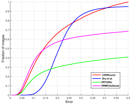
Figure 9: Average 3-pt error (normalized by eye-nose distance) vs fraction of images in the IJB-A dataset kumar_face_2016 .

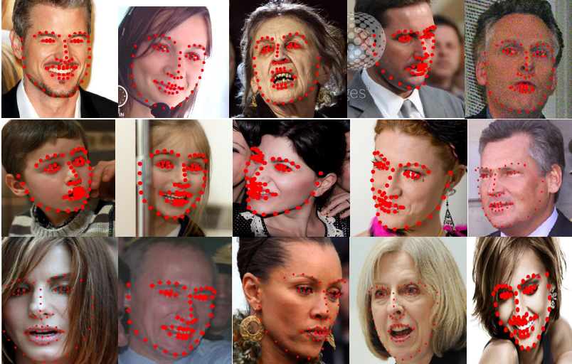
Figure 10: Sample facial landmark detection results.

4.3 IJB-A and JANUS CS2 for Face Verification

For face verification task, both IJB-A and JANUS CS2 datasets contain 500 subjects with 5,397 images and 2,042 videos split into 20,412 frames, 11.4 images and 4.2 videos per subject. Sample images and video frames from the datasets are shown in Figure 11. (i.e., the videos are only released for the JANUS CS2 dataset.) The IJB-A evaluation protocol consists of verification (1:1 matching) over 10 splits. Each split contains around 11,748 pairs of templates (1,756 positive and 9,992 negative pairs) on average. Similarly, the identification (1:N search) protocol also consists of 10 splits, which are used to evaluate the search performance. In each search split, there are about 112 gallery templates and 1,763 probe templates (i.e. 1,187 genuine probe templates and 576 impostor probe templates). On the other hand, for the JANUS CS2, there are about 167 gallery templates and 1,763 probe templates and all of them are used for both identification and verification. The training set for both datasets contains 333 subjects, and the test set contains 167 subjects without any overlapping subjects. Ten random splits of training and testing are provided by each benchmark, respectively. The main differences between IJB-A and JANUS CS2 evaluation protocols are that (1) IJB-A considers the open-set identification problem and the JANUS CS2 considers the closed-set identification and (2) IJB-A considers the more difficult pairs which are subsets of JANUS CS2 dataset.

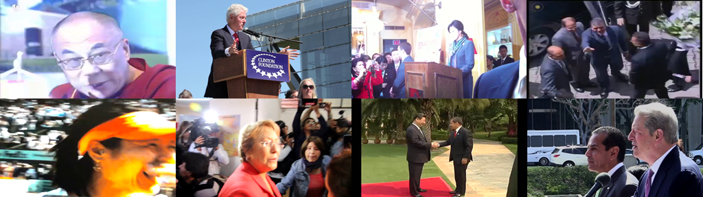
Figure 11: Sample images and frames from the IJB-A (top) and JANUS CS2 datasets (bottom). Challenging variations due to pose, illumination, resolution, occlusion, and image quality are present in these images.

Unlike the LFW and YTF datasets, which only use a sparse set of negative pairs to evaluate the verification performance, the IJB-A and JANUS CS2 datasets divide the images/video frames into gallery and probe sets so that all the available positive and negative pairs are used for the evaluation. Also, each gallery and probe set consist of multiple templates. Each template contains a combination of images or frames sampled from multiple image sets or videos of a subject. For example, the size of the similarity matrix for JANUS CS2 split1 is 167 $\times$ 1806 where 167 are for the gallery set and 1806 for the probe set (i.e. the same subject reappears multiple times in different probe templates). Moreover, some templates contain only one profile face with a challenging pose with low quality imagery. In contrast to LFW and YTF datasets, which only include faces detected by the Viola Jones face detector viola_robust_2004 , the images in the IJB-A and JANUS CS2 contain extreme pose, illumination, and expression variations. These factors essentially make the IJB-A and JANUS CS2 challenging face recognition datasets klare_janus_2015 .

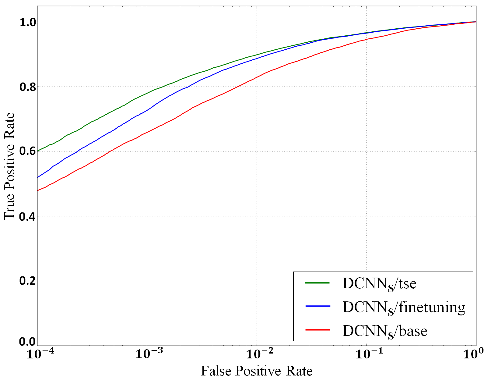
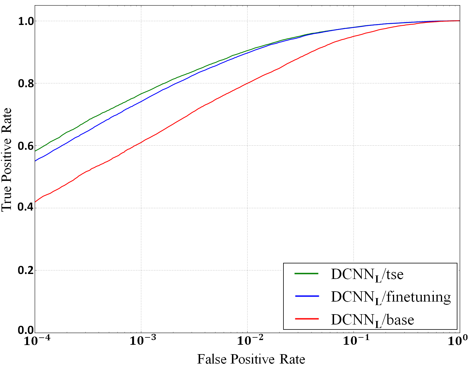
Figure 12: The performance evaluation for face verification tasks of (a) DCNN_S and (b) DCNN_L of before finetuning, with finetuning, and with finetuning and triplet similarity embedding for the JANUS CS2 dataset under Setup 3 (semi-automatic mode). Fine tuning is done only using the training data in each split.

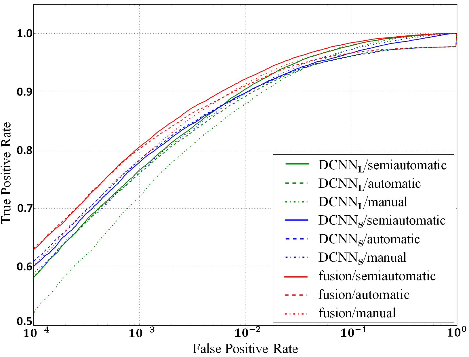
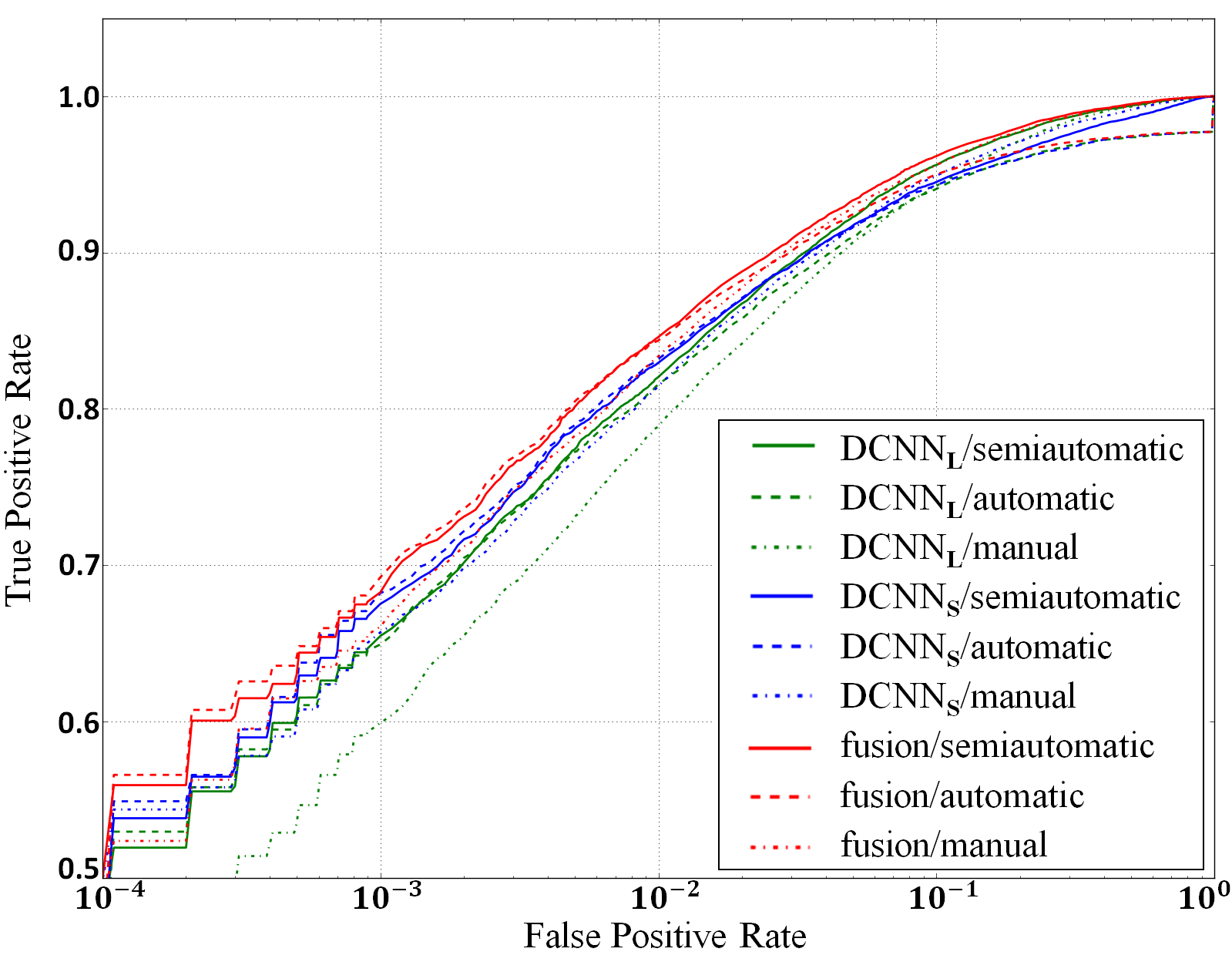
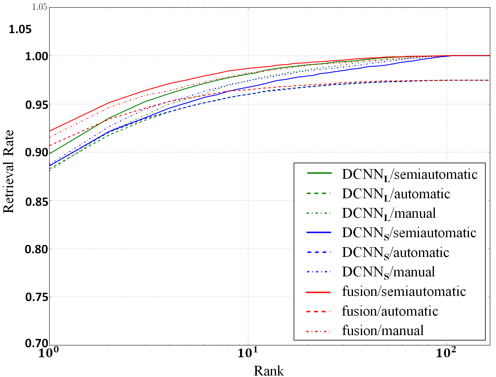
Figure 13: (a) and (b) show the face verification performance of the fusion model for JANUS CS2 and IJB-A (1:1) verification, respectively, and (c) shows the face identification performance of the fusion model for IJB-A (1:N) identification for all the three setups. Fine tuning is done only using the training data in each split.

4.4 Performance Evaluations of Face Verification on IJB-A and JANUS CS2

To take different situations into account, we have considered three modes of evaluations, manual, automatic and semi-automatic modes. This enables the handling of cases where we are unable to detect any of the faces (i.e., the failure of face detection.) in the images of the given template and also to compare the performance with the one using the metadata provided with the dataset. We describe the setups of performance evaluation in details as follows:

• Setup 1 (manual mode): Under this setup, we directly use the three facial landmarks and face bounding boxes provided along with the datasets.

• Setup 2 (automatic mode): In this setup when we get a video we use the face association method to detect and track the faces and to extract the bounding box to perform fiducial detection. If it is an image, we perform detection and facial landmark detection independently. For every image or frame in a template in which we are unable to detect the target face, we are unable to compare the template with others and thus assign all the corresponding entries for the template in the similarity matrices to the lowest similarity scores, -Inf.

• Setup 3 (semi-automatic mode): In this setup if we are able to detect the target face in an image then we follow setup 2. Otherwise, we follow setup 1 to use the metadata of the dataset for the faces which are not detected and tracked by our algorithms.

To evaluate the performance of two networks individually, we present the ROC curves of DCNN_S and DCNN_L of the Setup 3 (i.e., semi-automatic mode) for the JANUS CS2 dataset in Figure 12. As shown in the figures, the performances are consistently improved for both networks after fine-tuning the models previously trained using the CASIA-WebFace dataset on the training data of JANUS CS2. Triplet similarity embedding (TSE) further increase the performance for both networks, especially for the TAR number at the low FAR interval. For all the results presented here, fine tuning is done using only the training data in each split. The gallery dataset is not used for parameter fine tuning or for triplet similarity embedding. Then, we perform the fusion of the two networks by adding the corresponding similarity scores together and demonstrate the fusion results of all the three setup for the verification task of both JANUS CS2 and IJB-A in Figure  13 (a) and (b), respectively. In Figure  13 (c), we present the CMC curve for the IJB-A identification task. From Figure 13, it can be seen that even the simple fusion strategy used in this work significantly boosts the performance. Since DCNN_S is trained using tight face bounding boxes (DCNN_S) and DCNN_L using the large ones which includes more context (DCNN${}_{L})$, one possible reason for the performance improvement is that the two networks contain discriminative information learned from different scales and complement each other. In addition, the figure also shows that the performance of our system in Setup 2 (the automatic mode) is comparable to Setup 1 (the manual mode) and Setup 3 (the semi-automatic mode). This demonstrates the robustness of each component of our system.

IJB-A-Verif	DCNN (setup 1)	DCNN (setup 2)	DCNN (setup 3)	DCNNm (setup 1)	DCNNm (setup 2)	DCNNm (setup 3)
FAR=1e-2	0.834 $\pm$ 0.036	0.844 $\pm$ 0.026	0.846 $\pm$ 0.029	0.863 $\pm$ 0.02	0.885 $\pm$ 0.014	0.889 $\pm$ 0.016
FAR=1e-1	0.956 $\pm$ 0.008	0.95 $\pm$ 0.005	0.962 $\pm$ 0.007	0.966 $\pm$ 0.05	0.954 $\pm$ 0.003	0.968 $\pm$ 0.005
IJB-A-Ident	DCNN (setup 1)	DCNN (setup 2)	DCNN (setup 3)	DCNNm (setup 1)	DCNNm (setup 2)	DCNNm (setup 3)
Rank-1	0.915 $\pm$ 0.011	0.907 $\pm$ 0.011	0.922 $\pm$ 0.011	0.916 $\pm$ 0.009	0.923 $\pm$ 0.01	0.942 $\pm$ 0.008
Rank-5	0.969 $\pm$ 0.007	0.955 $\pm$ 0.007	0.975 $\pm$ 0.006	0.971 $\pm$ 0.007	0.961 $\pm$ 0.006	0.98 $\pm$ 0.005
Rank-10	0.982 $\pm$ 0.005	0.965 $\pm$ 0.005	0.987 $\pm$ 0.001	0.981 $\pm$ 0.005	0.969 $\pm$ 0.004	0.988 $\pm$ 0.003
IJB-A-Ident	DCNN (setup 1)	DCNN (setup 2)	DCNN (setup 3)	DCNNm (setup 1)	DCNNm (setup 2)	DCNNm (setup 3)
FPIR=0.01	0.618 $\pm$ 0.05	0.64 $\pm$ 0.043	0.631 $\pm$ 0.041	0.639 $\pm$ 0.057	0.646 $\pm$ 0.055	0.654 $\pm$ 0.001
FPIR=0.1	0.799 $\pm$ 0.014	0.806 $\pm$ 0.012	0.813 $\pm$ 0.014	0.816 $\pm$ 0.015	0.827 $\pm$ 0.012	0.836 $\pm$ 0.01

Table 5: Results on the IJB-A dataset. The TAR of all the approaches at FAR=0.1 and 0.01 for the ROC curves (IJB-A 1:1 verification). The Rank-1, Rank-5, and Rank-10 retrieval accuracies of the CMC curves and TPIR at FPIR = 0.01 and 0.1 (IJB-A 1:N identfication). We also show the results before and after media averaging where $m$ means media averaging.

CS2-Verif	DCNN (setup 1)	DCNN (setup 2)	DCNN (setup 3)	DCNNm (setup 1)	DCNNm (setup 2)	DCNNm (setup 3)
FAR=1e-2	0.913 $\pm$ 0.008	0.91 $\pm$ 0.008	0.922 $\pm$ 0.007	0.92 $\pm$ 0.01	0.922 $\pm$ 0.008	0.935 $\pm$ 0.007
FAR=1e-1	0.98 $\pm$ 0.004	0.967 $\pm$ 0.003	0.984 $\pm$ 0.003	0.981 $\pm$ 0.003	0.968 $\pm$ 0.003	0.986 $\pm$ 0.002
CS2-Ident	DCNN (setup 1)	DCNN (setup 2)	DCNN (setup 3)	DCNNm (setup 1)	DCNNm (setup 2)	DCNNm (setup 3)
Rank-1	0.9 $\pm$ 0.01	0.896 $\pm$ 0.008	0.909 $\pm$ 0.008	0.905 $\pm$ 0.007	0.915 $\pm$ 0.007	0.931 $\pm$ 0.007
Rank-5	0.963 $\pm$ 0.006	0.954 $\pm$ 0.006	0.969 $\pm$ 0.006	0.965 $\pm$ 0.004	0.959 $\pm$ 0.005	0.976 $\pm$ 0.004
Rank-10	0.977 $\pm$ 0.006	0.965 $\pm$ 0.004	0.981 $\pm$ 0.003	0.977 $\pm$ 0.004	0.967 $\pm$ 0.004	0.985 $\pm$ 0.002

Table 6: Results on the JANUS CS2 dataset. The TAR of all the approaches at FAR=0.1 and 0.01 for the ROC curves. The Rank-1, Rank-5, and Rank-10 retrieval accuracies of the CMC curves. We report average and standard deviation of the 10 splits. We also show the results before and after media averaging where $m$ means media averaging.

IJB-A-Verif	wang_face_2015	JanusB nist_ijba_2016	JanusD nist_ijba_2016	DCNNbl aruni_pose_2016	NAN yang_neural_2016	DCNN3d masi_neural_2016
FAR=1e-3	0.514 $\pm$ 0.006	0.65	0.49	-	0.785 $\pm$ 0.028	0.725
FAR=1e-2	0.732 $\pm$ 0.033	0.826	0.71	-	0.897 $\pm$ 0.01	0.886
FAR=1e-1	0.895 $\pm$ 0.013	0.932	0.89	-	0.959 $\pm$ 0.005	-
IJB-A-Ident	wang_face_2015	JanusB nist_ijba_2016	JanusD nist_ijba_2016	DCNNbl aruni_pose_2016	NAN yang_neural_2016	DCNN3d masi_neural_2016
Rank-1	0.820 $\pm$ 0.024	0.87	0.88	0.895 $\pm$ 0.011	-	0.906
Rank-5	0.929 $\pm$ 0.013	-	-	0.963 $\pm$ 0.005	-	0.962
Rank-10	-	0.95	0.97	-	-	0.977
IJB-A-Verif	DCNNpose AbdAlmageed_pose_2016	DCNNm (setup 1)	DCNNm (setup 2)	DCNNm (setup 3)	DCNN${tpe}$ swami_btas_2016	TP crosswhite_template_2016
FAR=1e-3	-	0.704 $\pm$ 0.037	0.762 $\pm$ 0.038	0.76 $\pm$ 0.038	0.813 $\pm$ 0.02	-
FAR=1e-2	0.787	0.863 $\pm$ 0.02	0.885 $\pm$ 0.014	0.889 $\pm$ 0.016	0.9 $\pm$ 0.01	0.939 $\pm$ 0.013
FAR=1e-1	0.911	0.966 $\pm$ 0.05	0.954 $\pm$ 0.003	0.968 $\pm$ 0.005	0.964 $\pm$ 0.01	-
IJB-A-Ident	DCNNpose AbdAlmageed_pose_2016	DCNNm (setup 1)	DCNNm (setup 2)	DCNNm (setup 3)	DCNN${tpe}$ swami_btas_2016	TP crosswhite_template_2016
Rank-1	0.846	0.916 $\pm$ 0.009	0.923 $\pm$ 0.01	0.942 $\pm$ 0.008	0.932 $\pm$ 0.001	0.928 $\pm$ 0.01
Rank-5	0.927	0.971 $\pm$ 0.007	0.961 $\pm$ 0.006	0.98 $\pm$ 0.005	-	-
Rank-10	0.947	0.981 $\pm$ 0.005	0.969 $\pm$ 0.004	0.988 $\pm$ 0.003	0.977 $\pm$ 0.005	0.986 $\pm$ 0.003

Table 7: Results on the IJB-A dataset. The TAR of all the approaches at FAR=0.1, 0.01, and 0.001 for the ROC curves (IJB-A 1:1 verification). The Rank-1, Rank-5, and Rank-10 retrieval accuracies of the CMC curves (IJB-A 1:N identfication). We report average and standard deviation of the 10 splits. All the performance results reported in nist_ijba_2016 , Janus B (JanusB-092015), Janus D (JanusD-071715), DCNN_bl aruni_pose_2016 , DCNN_3d masi_neural_2016 , NAN yang_neural_2016 , DCNN_pose AbdAlmageed_pose_2016 , DCNN_tpe swami_btas_2016 , and TP crosswhite_template_2016 are included in the Table. Some of these systems have produced results for setup 1 (based on landmarks provided along with the dataset) only. In addition, we also compare the performance of the recent work, DCNN_tpe swami_btas_2016 where the performance difference mainly comes from the better preprocessing module and improved metric, hyperface .

Besides using the average feature representation, we also perform media averaging which is to first average the features coming from the same media (image or video) and then further average the media average features to generate the final feature representation. We show the results before and after media averaging for both IJB-A and JANUS CS2 dataset in Table 5 and in Table 6 respectively. It is clear that media averaging significantly improves the performance.

Tables 7 and 8 summarize the scores (i.e., both ROC and CMC numbers) produced by different face verification methods on the IJB-A and JANUS CS2 datasets, respectively. For the IJB-A dataset, we compare our fusion results (i.e., we perform finetuning and TSE in Setup 3.) with DCNN_bl (bilinear CNN aruni_pose_2016 ), DCNN_pose (multi-pose DCNN models AbdAlmageed_pose_2016 ), NAN yang_neural_2016 , DCNN_3d masi_neural_2016 , template adaptation (TP) crosswhite_template_2016 , DCNN_tpe swami_btas_2016 and the ones nist_ijba_2016 reported recently by NIST where JanusB-092015 achieved the best verification results, and JanusD-071715 the best identification results. For the JANUS CS2 dataset, Table 8 includes, a DCNN-based method wang_face_2015 , Fisher vector-based method simonyan_fisher_2013 , DCNN_pose AbdAlmageed_pose_2016 , DCNN_3d masi_neural_2016 , and two commercial off-the-shelf matchers, COTS and GOTS klare_janus_2015 . From the ROC and CMC scores, we see that the fusion of DCNN methods significantly improve the performance. This can be attributed to the fact that the DCNN model does capture face variations over a large dataset and generalizes well to a new small dataset. In addition, the performance results of Janus B (Jan-usB-092015), Janus D (JanusD-071715), DCNN_bl and DCNN_pose systems have produced results for setup 1 (based on landmarks provided along with the dataset) only.

CS2-Verif	COTS	GOTS	FVsimonyan_fisher_2013	DCNNposeAbdAlmageed_pose_2016
FAR=1e-3	-	-	-	-
FAR=1e-2	0.581$\pm$0.054	0.467$\pm$0.066	0.411$\pm$0.081	0.897
FAR=1e-1	0.767$\pm$0.015	0.675$\pm$0.015	0.704$\pm$0.028	0.959
CS2-Ident	COTS	GOTS	FVsimonyan_fisher_2013	DCNNposeAbdAlmageed_pose_2016
Rank-1	0.551 $\pm$ 0.003	0.413 $\pm$ 0.022	0.381 $\pm$ 0.018	0.865
Rank-5	0.694 $\pm$ 0.017	0.571 $\pm$ 0.017	0.559 $\pm$ 0.021	0.934
Rank-10	0.741 $\pm$ 0.017	0.624 $\pm$ 0.018	0.637 $\pm$ 0.025	0.949
CS2-Verif	DCNN3d masi_neural_2016	DCNN (setup 1)	DCNN (setup 2)	DCNN (setup 3)
FAR=1e-3	0.824	0.81 $\pm$ 0.018	0.823 $\pm$ 0.013	0.83 $\pm$ 0.014
FAR=1e-2	0.926	0.92 $\pm$ 0.01	0.922 $\pm$ 0.008	0.935 $\pm$ 0.007
FAR=1e-1	-	0.981 $\pm$ 0.003	0.968 $\pm$ 0.003	0.986 $\pm$ 0.002
CS2-Ident	DCNN3d masi_neural_2016	DCNN (setup 1)	DCNN (setup 2)	DCNN (setup 3)
Rank-1	0.898	0.905 $\pm$ 0.007	0.915 $\pm$ 0.007	0.931 $\pm$ 0.007
Rank-5	0.956	0.965 $\pm$ 0.004	0.959 $\pm$ 0.005	0.976 $\pm$ 0.004
Rank-10	0.969	0.977 $\pm$ 0.004	0.967 $\pm$ 0.004	0.985 $\pm$ 0.002

Table 8: Results on the JANUS CS2 dataset. The TAR of all the approaches at FAR=0.1, 0.01, and 0.001 for the ROC curves. The Rank-1, Rank-5, and Rank-10 retrieval accuracies of the CMC curves. We report average and standard deviation of the 10 splits. The performance results of DCNN_pose have produced results for setup 1 only.

During the review period of the paper, newer results on IJB-A datasets have been reported. The interested readers are referred to xiong2017good ; ranjan2017l2 for more details. In addition, the NAN yang2017neural results are based on an earlier version yang_neural_2016 . More recent state of the art results are reported in ranjan2017l2 obtained by employing the deep residual network and $L_{2}$-norm regularized softmax loss.

4.5 Labeled Faces in the Wild

We also evaluate our approach on the well-known LFW dataset huang_labeled_2008 using the standard protocol which defines 3,000 positive pairs and 3,000 negative pairs in total and further splits them into 10 disjoint subsets for cross validation. Each subset contains 300 positive and 300 negative pairs. It contains 7,701 images of 4,281 subjects. We compare the mean accuracy of the proposed deep model with other state-of-the-art deep learning-based methods: DeepFace taigman_deepface_2014 , DeepID2 sun_deeply_2014 , DeepID3 sun_deepid3_2015 , FaceNet schroff_facenet_2015 , Yi et al. yi_learning_2014 , Wang et al. wang_face_2015 , Ding et al. ding_robust_2015 , Parkhi et al. parkhi_deep_2015 , and human performance on the “funneled” LFW images. The results are summarized in Table  9. It can be seen that our approach performs comparable to other deep learning-based methods. Note that some of the deep learning-based methods compared in Table 9 use millions of data samples for training the model. In comparison, we use only the CASIA dataset for training our model which has less than 500K images.

Method	#Net	Training Set	Metric	Mean Accuracy $\pm$ Std
DeepFace taigman_deepface_2014	1	4.4 million images of 4,030 subjects, private	cosine	95.92% $\pm$ 0.29%
DeepFace	7	4.4 million images of 4,030 subjects, private	unrestricted, SVM	97.35% $\pm$ 0.25%
DeepID2 sun_deeply_2014	1	202,595 images of 10,117 subjects, private	unrestricted, Joint-Bayes	95.43%
DeepID2	25	202,595 images of 10,117 subjects, private	unrestricted, Joint-Bayes	99.15% $\pm$ 0.15%
DeepID3 sun_deepid3_2015	50	202,595 images of 10,117 subjects, private	unrestricted, Joint-Bayes	99.53% $\pm$ 0.10%
FaceNet schroff_facenet_2015	1	260 million images of 8 million subjects, private	L2	99.63% $\pm$ 0.09%
Yi et al. yi_learning_2014	1	494,414 images of 10,575 subjects, public	cosine	96.13% $\pm$ 0.30%
Yi et al.	1	494,414 images of 10,575 subjects, public	unrestricted, Joint-Bayes	97.73% $\pm$ 0.31%
Wang et al. wang_face_2015	1	494,414 images of 10,575 subjects, public	cosine	96.95% $\pm$ 1.02%
Wang et al.	7	494,414 images of 10,575 subjects, public	cosine	97.52% $\pm$ 0.76%
Wang et al.	1	494,414 images of 10,575 subjects, public	unrestricted, Joint-Bayes	97.45% $\pm$ 0.99%
Wang et al.	7	494,414 images of 10,575 subjects, public	unrestricted, Joint-Bayes	98.23% $\pm$ 0.68%
Ding et al. ding_robust_2015	8	471,592 images of 9,000 subjects, public	unrestricted, Joint-Bayes	99.02% $\pm$ 0.19%
Parkhi et al. parkhi_deep_2015	1	2.6 million images of 2,622 subjects, public	unrestricted, TDE	98.95 %
Human, funneled wang_face_2015	N/A	N/A	N/A	99.20%
Our DCNNS	1	490,356 images of 10,548 subjects, public	cosine	97.7% $\pm$ 0.8%
Our DCNNL	1	490,356 images of 10,548 subjects, public	cosine	96.8% $\pm$ 0.6%
Our DCNNS + DCNNL	2	490,356 images of 10,548 subjects, public	cosine	98% $\pm$ 0.5%
Our DCNNS + DCNNL	2	490,356 images of 10,548 subjects, public	unrestricted, TSE	98.33% $\pm$ 0.7%

Table 9: Accuracy of different methods on the LFW dataset.

4.6 Comparison with Methods based on Annotated Metadata

Most systems compared in this paper produced the results for setup 1 which is based on landmarks provided along with the dataset only (i.e., except DCNN_tpe.). For DCNN_3d masi_neural_2016 , the number of face images is augmented along with the original CASIA-WebFace dataset by aro-und 2 million using 3D morphable models. On the other hand, NAN yang_neural_2016 and TP crosswhite_template_2016 used datasets with more than 2 million face images to train the model. However, the networks used in this work were trained with the original CASIA-WebFace which contains around 500K images. In addition, TP adapted the one-shot similarity framework wolf2009one with linear support vector machine for set-based face verification and trained the metric on-the-fly with the help of a pre-selected negative set during testing. Although TP achieved significantly better results than other approaches, it takes more time during testing than the proposed method since our metric is trained off-line and requires much less time for testing than TP. We expect the performance of the proposed approach can also be improved by using the one-shot similarity framework. As shown in Table 7, the proposed approach achieves comparable results to other methods and strikes a balance between testing time and performance. In a recent work, DCNN_tpe swami_btas_2016 , adopted a probabilistic embedding for similarity computation and a new face preprocessing module, hyperface hyperface , for improved face detection and fiducials where hyperface is a multi-task deep network trained for the tasks of gender classification, fiducial detection, pose estimation and face detection. We plan to incorporate hyperface into the current framework which may yield some improvement in performance.

4.7 Run Time

The DCNN_S model for face verification is trained on the CASIA-Webface dataset from scratch for about 4 days and for DCNN_L, it takes 20 hours to train on the same face dataset which is initialized using the weights of Alexnet pretrained on the ImageNet dataset. The two networks are trained using NVidia Titan X with cudnn v4. The running time for face detection is around 0.7 second per image. The facial landmark detection and feature extraction steps take about 1 second and 0.006 second per face, respectively (i.e., To compare the speed difference, we run the feature extraction part using CPU. it takes around 0.7 second for feature extraction using a core of 16-core 3.0GHz Intel Xeon CPU and math library atlas which is around 100 times as the GPU time.) The face association module for a video takes around 5 fps on average.

5 Open Issues

Given sufficient number of annotated data and GPUs, DCNNs have been shown to yield impressive performance improvements. Still many issues remain to be addressed to make the DCNN-based recognition systems robust and practical. These are briefly discussed below.

• Reliance on large training data sets: One of the top performing networks in the MegaFace challenge needs 500 million faces of about 10 million subjects. Such large annotated training set may not be always available (e.g. expression recognition, age estimation). So networks that can perform well with reasonable-sized training data are needed.

• Invariance: While limited invariance to translation is possible with existing DCNNs, networks that can incorporate more general invariances are needed.

• Training time: The training time even when GPUs are used can be several tens of hours, depending on the number of layers used and the training data size. More efficient implementations of learning algorithms, preferably implemented using CPUs are desired.

• Number of parameters: The number of parameters can be several tens of millions. Novel strategies that reduce the number of parameters need to be developed.

• Handling degradations in training data: : DCNNs robust to low-resolution, blur, illumination and pose variations, occlusion, erroneous annotation, etc. are needed to handle degradations in data.

• Domain adaptation of DCNNs: While having large volumes of data may help with processing test data from a different distribution than that of the training data, systematic methods for adapting the deep features to test data are needed.

• Theoretical considerations: While DCNNs have been around for a few years, detailed theoretical understanding is just starting to develop bruna_invariant_2013 ; mallat_understanding_2016 ; Raja_deep ; vidal_deep . Methods for deciding the number of layers, neighborhoods over which max pooling operations are performed are needed.

• Incorporating domain knowledge: The current practice is to rely on fine tuning. For example, for the age estimation problem, one can start with one of the standard networks such as the AlexNet and fine tune it using aging data. While this may be reasonable for somewhat related problems (face recognition and facial expression recognition), such fine tuning strategies may not always be effective. Methods that can incorporate context may make the DCNNs more applicable to a wider variety of problems.

• Memory: Although Recurrent CNNs are on the rise, they still consume a lot of time and memory for training and deployment. Efficient DCNN algorithms are needed to handle videos and other data streams as blocks.

We also discussed design considerations for each component of a full face verification system, including

• Face detection: Face detection is challenging due to the wide range of variations in the appearance of faces. The variability is caused mainly by changes in illumination, facial expression, viewpoints, occlusions, etc. Other factors such as blurry images and low resolution are prominent in face detection task.

• Fiducial detection: Most of the datasets only contain few thousands images. A large scale annotated and unconstrained dataset will make the face alignment system more robust to the challenges, including extreme pose, low illumination, small and blurry face images. Researchers have hypothesized that deeper layers can encode more abstract information such as identity, pose, and attributes; However, it has not yet been thoroughly studied which layers exactly correspond to local features for fiducial detection.

• Face association: Since the video clips may contain media of low-quality images, the blurred and low-resolution image makes the face detection not reliable. This may lead to performance degradation of face association since a face track will not be initiated due to the missing of face detection. Besides, abrupt motion, occlusion, and crowded scene can lead to performance degradation of tracking and potential identity switching.

• Face verification: For face verification, the performance can be improved by learning a discriminative distance measure. However, due to memory constraints limited by graphics cards, how to choose informative pairs or triplets and train the network end-to-end using online methods (e.g., stochastic gradient descent) on large-scale datasets are still open problems.

6 Conclusion

We presented the design and performance of our automatic face verification system, which automatically locates faces and performs verification/recognition on newly released challenging face verification datasets, IARPA Benchmark A (IJB-A) and its extended version, JANUS CS2. It is shown that the proposed DCNN-based system can not only accurately locate the faces across images and videos but also learn a robust model for face verification. Experimental results demonstrate that the performance of the proposed system on the IJB-A dataset is much better than a FV-based method and some COTS and GOTS matchers.

7 Acknowledgments

This research is based upon work supported by the Office of the Director of National Intelligence (ODNI), Intelligence Advanced Research Projects Activity (IARPA), via IARPA R&D Contract No. 2014-14071600012. The views and conclusions contained herein are those of the authors and should not be interpreted as necessarily representing the official policies or endorsements, either expressed or implied, of the ODNI, IARPA, or the U.S. Government. The U.S. Government is authorized to reproduce and distribute reprints for Governmental purposes notwithstanding any copyright annotation thereon. We thank professor Alice O’Toole for carefully reading the manuscript and suggesting improvements in the presentation of this work.

References

- (1) National institute of standards and technology (NIST): IARPA Janus benchmark-a performance report. URL \urlhttp://biometrics.nist.gov/cs_links/face/face_challenges/IJBA_reports.zip
- (2) AbdAlmageed, W., Wu, Y., Rawls, S., Harel, S., Hassne, T., Masi, I., Choi, J., Lekust, J., Kim, J., Natarajana, P., Nevatia, R., Medioni, G.: Face recognition using deep multi-pose representations. In: IEEE Winter Conference on Applications of Computer Vision (WACV) (2016)
- (3) Ahonen, T., Hadid, A., Pietikainen, M.: Face description with local binary patterns: Application to face recognition. IEEE Transactions on Pattern Analysis and Machine Intelligence 28(12), 2037–2041 (2006)
- (4) Ahuja, R., Magnanti, T., Orlin, J.: Network Flows: Theory, Algorithms, and Applications. Prentice Hall (1993)
- (5) Asthana, A., Zafeiriou, S., Cheng, S., Pantic, M.: Robust discriminative response map fitting with constrained local models. In: IEEE Conference on Computer Vision and Pattern Recognition, pp. 3444–3451 (2013)
- (6) Asthana, A., Zafeiriou, S., Cheng, S.Y., Pantic, M.: Robust discriminative response map fitting with constrained local models. In: IEEE Conference on Computer Vision and Pattern Recognition, pp. 3444–3451 (2013)
- (7) Babenko, B., Yang, M.H., Belongie, S.: Visual tracking with online multiple instance learning. In: IEEE Conference on Computer Vision and Pattern Recognition (CVPR), pp. 983–990. IEEE (2009)
- (8) Bae, S.H., Yoon, K.J.: Robust online multi-object tracking based on tracklet confidence and online discriminative appearance learning. IEEE Conference on Computer Vision and Pattern Recognition (CVPR) (2014)
- (9) Belhumeur, P.N., Jacobs, D.W., Kriegman, D.J., Kumar, N.: Localizing parts of faces using a consensus of exemplars. IEEE Transactions on Pattern Analysis and Machine Intelligence 35(12), 2930–2940 (2013)
- (10) Bodla, N., Zheng, J., Xu, H., Chen, J.C., Castillo, C.D., Chellappa, R.: Deep heterogeneous feature fusion for template-based face recognition. IEEE Winter Conference on Applications of Computer Vision (WACV) (2017)
- (11) Breitenstein, M.D., Reichlin, F., Leibe, B., Koller-Meier, E., Gool, L.V.: Robust tracking-by-detection using a detector confidence particle filter. IEEE International Conference on Computer Vision (ICCV) (2009)
- (12) Bruna, J., Mallat, S.: Invariant scattering convolution networks. IEEE Transactions on Pattern Analysis and Machine Intelligence 35(8), 1872–1886 (2013)
- (13) Burgos-Artizzu, X.P., Perona, P., Dollár, P.: Robust face landmark estimation under occlusion
- (14) Cao, X., Wei, Y., Wen, F., Sun, J.: Face alignment by explicit shape regression (2014). URL \urlhttp://www.google.com/patents/US20140185924. US Patent App. 13/728,584
- (15) Chen, D., Cao, X.D., Wang, L.W., Wen, F., Sun, J.: Bayesian face revisited: A joint formulation. In: European Conference on Computer Vision, pp. 566–579 (2012)
- (16) Chen, D., Cao, X.D., Wen, F., Sun, J.: Blessing of dimensionality: High-dimensional feature and its efficient compression for face verification. In: IEEE Conference on Computer Vision and Pattern Recognition (2013)
- (17) Chen, J.C., Patel, V.M., Chellappa, R.: Unconstrained face verification using deep cnn features. arXiv preprint arXiv:1508.01722 (2015)
- (18) Chen, J.C., Ranjan, R., Kumar, A., Chen, C.H., Patel, V.M., Chellappa, R.: An end-to-end system for unconstrained face verification with deep convolutional neural networks. In: IEEE International Conference on Computer Vision Workshop on ChaLearn Looking at People, pp. 118–126 (2015)
- (19) Chen, J.C., Sankaranarayanan, S., Patel, V.M., Chellappa, R.: Unconstrained face verification using Fisher vectors computed from frontalized faces. In: IEEE International Conference on Biometrics: Theory, Applications and Systems (2015)
- (20) Chen, Y.C., Patel, V.M., Phillips, P.J., Chellappa, R.: Dictionary-based face recognition from video. European Conference on Computer Vision (ECCV) (2012)
- (21) Cheney, J., Klein, B., Jain, A.K., Klare, B.F.: Unconstrained face detection: State of the art baseline and challenges. In: International Conference on Biometrics (2015)
- (22) Comaschi, F., Stuijk, S., Basten, T., Corporaal, H.: Online multi-face detection and tracking using detector confidence and structured SVMs. IEEE International Conference on Advanced Video and Signal based Surveillance (AVSS) (2015)
- (23) Cootes, T.F., Edwards, G.J., Taylor, C.J.: Active appearance models. IEEE Transactions on Pattern Analysis and Machine Intelligence (6), 681–685 (2001)
- (24) Cootes, T.F., Taylor, C.J., Cooper, D.H., Graham, J.: Active shape models-their training and application. Computer vision and image understanding 61(1), 38–59 (1995)
- (25) Cristinacce, D., Cootes, T.F.: Feature detection and tracking with constrained local models. In: British Machine Vision Conference, vol. 1, p. 3 (2006)
- (26) Crosswhite, N., Byrne, J., Parkhi, O.M., Stauffer, C., Cao, Q., Zisserman, A.: Template adaptation for face verification and identification. arXiv preprint arXiv:1603.03958 (2016)
- (27) D. Chen S. Ren, Y.W.X.C., Sun, J.: Joint cascade face detection and alignment. In: D. Fleet, T. Pajdla, B. Schiele, T. Tuytelaars (eds.) European Conference on Computer Vision, vol. 8694, pp. 109–122 (2014)
- (28) Davis, J.V., Kulis, B., Jain, P., Sra, S., Dhillon, I.S.: Information-theoretic metric learning. In: International Conference on Machine learning, pp. 209–216 (2007)
- (29) Ding, C., Tao, D.: Robust face recognition via multimodal deep face representation. arXiv preprint arXiv:1509.00244 (2015)
- (30) Dollár, P., Welinder, P., Perona, P.: Cascaded pose regression. In: IEEE Conference on Computer Vision and Pattern Recognition, pp. 1078–1085. IEEE (2010)
- (31) Donahue, J., Jia, Y., Vinyals, O., Hoffman, J., Zhang, N., Tzeng, E., Darrell, T.: Decaf: A deep convolutional activation feature for generic visual recognition. arXiv preprint arXiv:1310.1531 (2013)
- (32) Du, M., Chellappa, R.: Face association across unconstrained video frames using conditional random fields. European Conference on Computer Vision (ECCV) (2012)
- (33) Duffner, S., Odobez, J.: Track creation and deletion framework for long-term online multiface tracking. IEEE Transactions on Image Processing 22(1), 272–285 (2013)
- (34) Everingham, M., Gool, L.V., Williams, C.K.I., Winn, J., Zisserman, A.: The pascal visual object classes (VOC) challenge. International Journal of Computer Vision 88(2), 303–338 (2009)
- (35) Farfade, S.S., Saberian, M.J., Li, L.J.: Multi-view face detection using deep convolutional neural networks. In: International Conference on Multimedia Retrieval (2015)
- (36) Girshick, R., Donahue, J., Darrell, T., Malik, J.: Rich feature hierarchies for accurate object detection and semantic segmentation. In: IEEE Conference on Computer Vision and Pattern Recognition, pp. 580–587 (2014)
- (37) Girshick, R., Iandola, F., Darrell, T., Malik, J.: Deformable part models are convolutional neural networks. IEEE Conference on Computer Vision and Pattern Recognition (2014)
- (38) Giryes, R., Sapiro, G., Bronstein, A.M.: On the stability of deep networks. arXiv preprint arXiv:1412.5896 (2014)
- (39) Gross, R., Matthews, I., Cohn, J., Kanade, T., Baker, S.: Multi-pie. Image and Vision Computing 28(5), 807–813 (2010)
- (40) Guillaumin, M., Verbeek, J., Schmid, C.: Is that you? metric learning approaches for face identification. In: IEEE International Conference on Computer Vision, pp. 498–505 (2009)
- (41) Haeffele, B.D., Vidal, R.: Global optimality in tensor factorization, deep learning, and beyond. arXiv preprint arXiv:1506.07540 (2015)
- (42) Hassner, T., Harel, S., Paz, E., Enbar, R.: Effective face frontalization in unconstrained images. In: IEEE Conference on Computer Vision and Pattern Recognition(CVPR), pp. 4295–4304 (2015)
- (43) He, K., Zhang, X., Ren, S., Sun, J.: Delving deep into rectifiers: Surpassing human-level performance on imagenet classification. arXiv preprint arXiv:1502.01852 (2015)
- (44) Henriques, J.F., Caseiro, R., Martins, P., Batista, J.: High-speed tracking with kernelized correlation filters. IEEE Transactions on Pattern Analysis and Machine Intelligence 37(3), 583–596 (2015)
- (45) Hu, J., Lu, J., Tan, Y.P.: Discriminative deep metric learning for face verification in the wild. In: IEEE Conference on Computer Vision and Pattern Recognition, pp. 1875–1882 (2014)
- (46) Huang, C., Wu, B., Nevatia, R.: Robust object tracking by hierarchical association of detection responses. European Conference on Computer Vision (ECCV) (2008)
- (47) Huang, G.B., Mattar, M., Berg, T., Learned-Miller, E.: Labeled faces in the wild: A database forstudying face recognition in unconstrained environments. In: Workshop on Faces in Real-Life Images: Detection, Alignment, and Recognition (2008)
- (48) Jain, V., Learned-Miller, E.: Fddb: A benchmark for face detection in unconstrained settings. UM-CS-2010-009 (2010)
- (49) Kalal, Z., Mikolajczyk, K., Matas, J.: Tracking-learning-detection. IEEE Transactions on Pattern Analysis and Machine Intelligence 34(7), 1409–1422 (2012)
- (50) Kazemi, V., Sullivan, J.: One millisecond face alignment with an ensemble of regression trees. In: IEEE Conference on Computer Vision and Pattern Recognition, pp. 1867–1874 (2014)
- (51) Klare, B.F., Klein, B., Taborsky, E., Blanton, A., Cheney, J., Allen, K., Grother, P., Mah, A., Burge, M., Jain, A.K.: Pushing the frontiers of unconstrained face detection and recognition: IARPA Janus Benchmark A. In: IEEE Conference on Computer Vision and Pattern Recognition (2015)
- (52) Krizhevsky, A., Sutskever, I., Hinton, G.E.: Imagenet classification with deep convolutional neural networks. In: Advances in Neural Information Processing Systems, pp. 1097–1105 (2012)
- (53) Kumar, A., Ranjan, R., Patel, V., Chellappa, R.: Face alignment by local deep descriptor regression. arXiv preprint arXiv:1601.07950 (2016)
- (54) Le, V., Brandt, J., Lin, Z., Bourdev, L., Huang, T.S.: Interactive facial feature localization. In: European Conference on Computer Vision, pp. 679–692. Springer (2012)
- (55) Li, H., Hua, G., Lin, Z., Brandt, J., Yang, J.: Probabilistic elastic part model for unsupervised face detector adaptation. In: IEEE International Conference on Computer Vision, pp. 793–800 (2013)
- (56) Li, H., Lin, Z., Shen, X., Brandt, J., Hua, G.: A convolutional neural network cascade for face detection. In: IEEE Conference on Computer Vision and Pattern Recognition, pp. 5325–5334 (2015)
- (57) Li, J., Zhang, Y.: Learning surf cascade for fast and accurate object detection. In: Computer Vision and Pattern Recognition (CVPR), 2013 IEEE Conference on, pp. 3468–3475 (2013). DOI 10.1109/CVPR.2013.445
- (58) Liao, S., Jain, A.K., Li, S.Z.: A fast and accurate unconstrained face detector. IEEE transactions on pattern analysis and machine intelligence 38(2), 211–223 (2016)
- (59) Long, M., Wang, J.: Learning transferable features with deep adaptation networks. arXiv preprint arXiv:1502.02791 (2015)
- (60) Lui, Y.M., R.Beveridge, J., Whitley, L.D.: Adaptive appearance model and condensation algorithm for robust face tracking. IEEE Transactions on Systems, Man, and Cybernetics-Part A: Systems and Humans 40(3), 437–448 (2010)
- (61) Mallat, S.: Understanding deep convolutional networks. arXiv preprint arXiv:1601.04920 (2016)
- (62) Masi, I., Tran, A.T., Leksut, J.T., Hassner, T., Medioni, G.: Do we really need to collect millions of faces for effective face recognition? arXiv preprint arXiv:1603.07057 (2016)
- (63) Mathias, M., Benenson, R., Pedersoli, M., Gool, L.V.: Face detection without bells and whistles. In: European Conference on Computer Vision, vol. 8692, pp. 720–735 (2014)
- (64) Mignon, A., Jurie, F.: Pcca: A new approach for distance learning from sparse pairwise constraints. In: IEEE Conference on Computer Vision and Pattern Recognition (CVPR), pp. 2666–2672 (2012)
- (65) Nguyen, H.V., Bai, L.: Cosine similarity metric learning for face verification. In: Asian Conference on Computer Vision, pp. 709–720. Springer (2010)
- (66) Parkhi, O.M., Vedaldi, A., Zisserman, A.: Deep face recognition. British Machine Vision Conference (2015)
- (67) Ranjan, R., Castillo, C.D., Chellappa, R.: L2-constrained softmax loss for discriminative face verification. arXiv preprint arXiv:1703.09507 (2017)
- (68) Ranjan, R., Patel, V.M., Chellappa, R.: A deep pyramid deformable part model for face detection. In: IEEE International Conference on Biometrics: Theory, Applications and Systems (2015)
- (69) Ranjan, R., Patel, V.M., Chellappa, R.: HyperFace: A Deep Multi-task Learning Framework for Face Detection, Landmark Localization, Pose Estimation, and Gender Recognition (2016). URL \urlhttp://arxiv.org/abs/1603.01249
- (70) Ranjan, R., Sankaranarayanan, S., Castillo, C.D., Chellappa, R.: An all-in-one convolutional neural network for face analysis. arXiv preprint arXiv:1611.00851 (2016)
- (71) Ren, S., Cao, X., Wei, Y., Sun, J.: Face alignment at 3000 fps via regressing local binary features. In: IEEE Conference on Computer Vision and Pattern Recognition (CVPR), pp. 1685–1692 (2014). DOI 10.1109/CVPR.2014.218
- (72) Ross, G.: Fast r-cnn. In: IEEE International Conference on Computer Vision, pp. 1440–1448 (2015)
- (73) Roth, M., Bauml, M., Nevatia, R., Stiefelhagen, R.: Robust multi-pose face tracking by multi-stage tracklet association. International Conference on Pattern Recognition (ICPR) (2012)
- (74) RoyChowdhury, A., Lin, T.Y., Maji, S., Learned-Miller, E.: One-to-many face recognition with bilinear cnns. In: IEEE Winter Conference on Applications of Computer Vision (WACV) (2016)
- (75) Sankaranarayanan, S., Alavi, A., Castillo, C.D., Chellappa, R.: Triplet probabilistic embedding for face verification and clustering. In: IEEE International Conference on Biometrics Theory, Applications and Systems (BTAS), 2016, pp. 1–8 (2016)
- (76) Sankaranarayanan, S., Alavi, A., Chellappa, R.: Triplet similarity embedding for face verification. arXiv preprint arXiv:1602.03418 (2016)
- (77) Schroff, F., Kalenichenko, D., Philbin, J.: Facenet: A unified embedding for face recognition and clustering. arXiv preprint arXiv:1503.03832 (2015)
- (78) Shi, J., Tomasi, C.: Good features to track. IEEE Conference on Computer Vision and Pattern Recognition (CVPR) (1994)
- (79) Simonyan, K., Parkhi, O.M., Vedaldi, A., Zisserman, A.: Fisher vector faces in the wild. In: British Machine Vision Conference, vol. 1, p. 7 (2013)
- (80) Simonyan, K., Zisserman, A.: Very deep convolutional networks for large-scale image recognition. arXiv preprint arXiv:1409.1556 (2014)
- (81) Sun, Y., Liang, D., Wang, X., Tang, X.: Deepid3: Face recognition with very deep neural networks. arXiv preprint arXiv:1502.00873 (2015)
- (82) Sun, Y., Wang, X., Tang, X.: Deep convolutional network cascade for facial point detection. In: IEEE Conference on Computer Vision and Pattern Recognition, pp. 3476–3483 (2013)
- (83) Sun, Y., Wang, X., Tang, X.: Deeply learned face representations are sparse, selective, and robust. arXiv preprint arXiv:1412.1265 (2014)
- (84) Szegedy, C., Liu, W., Jia, Y., Sermanet, P., Reed, S., Anguelov, D., Erhan, D., Vanhoucke, V., Rabinovich, A.: Going deeper with convolutions. arXiv preprint arXiv:1409.4842 (2014)
- (85) Taigman, Y., Wolf, L., Hassner, T.: Multiple one-shots for utilizing class label information. In: British Machine Vision Conference, pp. 1–12 (2009)
- (86) Taigman, Y., Yang, M., Ranzato, M.A., Wolf, L.: Deepface: Closing the gap to human-level performance in face verification. In: IEEE Conference on Computer Vision and Pattern Recognition, pp. 1701–1708 (2014)
- (87) Tzimiropoulos, G., Pantic, M.: Gauss-newton deformable part models for face alignment in-the-wild. In: IEEE Conference on Computer Vision and Pattern Recognition (CVPR), pp. 1851–1858 (2014). DOI 10.1109/CVPR.2014.239
- (88) Viola, P., Jones, M.J.: Robust real-time face detection. International journal of computer vision 57(2), 137–154 (2004)
- (89) Wang, D., Otto, C., Jain, A.K.: Face search at scale: 80 million gallery. arXiv preprint arXiv:1507.07242 (2015)
- (90) Wang, P., Ji, Q.: Robust face tracking via collaboration of generic and specific models. IEEE Transactions on Image Processing 17(7), 1189–1199 (2008)
- (91) Weinberger, K.Q., Blitzer, J., Saul, L.K.: Distance metric learning for large margin nearest neighbor classification. In: Advances in neural information processing systems, pp. 1473–1480 (2006)
- (92) Wolf, L., Hassner, T., Taigman, Y.: The one-shot similarity kernel. In: International Conference on Computer Vision, pp. 897–902. IEEE (2009)
- (93) Xiong, L., Karlekar, J., Zhao, J., Feng, J., Pranata, S., Shen, S.: A good practice towards top performance of face recognition: Transferred deep feature fusion. arXiv preprint arXiv:1704.00438 (2017)
- (94) Xiong, X., la Torre, F.D.: Supervised descent method and its applications to face alignment. In: Computer Vision and Pattern Recognition (CVPR), 2013 IEEE Conference on, pp. 532–539 (2013). DOI 10.1109/CVPR.2013.75
- (95) Yan, J., Zhang, X., Lei, Z., Li, S.Z.: Face detection by structural models. Image and Vision Computing 32(10), 790 – 799 (2014). DOI http://dx.doi.org/10.1016/j.imavis.2013.12.004. URL \urlhttp://www.sciencedirect.com/science/article/pii/S0262885613001765. Best of Automatic Face and Gesture Recognition 2013
- (96) Yang, B., Yan, J., Lei, Z., Li, S.Z.: Convolutional channel features. In: IEEE International Conference on Computer Vision (2015)
- (97) Yang, J., Ren, P., Chen, D., Wen, F., Li, H., Hua, G.: Neural aggregation network for video face recognition. arXiv preprint arXiv:1603.05474 (2016)
- (98) Yang, J., Ren, P., Zhang, D., Chen, D., Wen, F., Li, H., Hua, G.: Neural aggregation network for video face recognition. In: IEEE Conference on Computer Vision and Pattern Recognition (CVPR) (2017)
- (99) Yang, S., Luo, P., Loy, C.C., Tang, X.: From facial parts responses to face detection: A deep learning approach. IEEE International Conference on Computer Vision (2015)
- (100) Yi, D., Lei, Z., Liao, S., Li, S.Z.: Learning face representation from scratch. arXiv preprint arXiv:1411.7923 (2014)
- (101) Yoon, J.H., Yang, M.H., Lim, J., Yoon, K.J.: Bayesian multi-object tracking using motion context from multiple objects. IEEE Winter Conference on Applications of Computer Vision (WACV) (2015)
- (102) Yosinski, J., Clune, J., Bengio, Y., Lipson, H.: How transferable are features in deep neural networks? In: Advances in Neural Information Processing Systems, pp. 3320–3328 (2014)
- (103) Zhang, J., Shan, S., Kan, M., Chen, X.: Coarse-to-fine auto-encoder networks (CFAN) for real-time face alignment. In: European Conference on Computer Vision ECCV, pp. 1–16 (2014). DOI 10.1007/978-3-319-10605-2_1. URL \urlhttp://dx.doi.org/10.1007/978-3-319-10605-2_1
- (104) Zhao, W.Y., Chellappa, R., Phillips, P.J., Rosenfeld, A.: Face recognition: A literature survey. ACM Computing Surveys 35(4), 399–458 (2003)
- (105) Zhu, S., Li, C., Chen, C.L., Tang, X.: Face alignment by coarse-to-fine shape searching. In: IEEE Conference on Computer Vision and Pattern Recognition (CVPR) (2015)
- (106) Zhu, X., Ramanan, D.: Face detection, pose estimation, and landmark localization in the wild. In: IEEE Conference on Computer Vision and Pattern Recognition (CVPR), pp. 2879–2886. IEEE (2012)