Exact ICL maximization in a non-stationary temporal extension of the stochastic block model for dynamic networks

Abstract

The stochastic block model (SBM) is a flexible probabilistic tool that can be used to model interactions between clusters of nodes in a network. However, it does not account for interactions of time varying intensity between clusters. The extension of the SBM developed in this paper addresses this shortcoming through a temporal partition: assuming interactions between nodes are recorded on fixed-length time intervals, the inference procedure associated with the model we propose allows to cluster simultaneously the nodes of the network and the time intervals. The number of clusters of nodes and of time intervals, as well as the memberships to clusters, are obtained by maximizing an exact integrated complete-data likelihood, relying on a greedy search approach. Experiments on simulated and real data are carried out in order to assess the proposed methodology.

1 Introduction

Network analysis has been applied since the 30s to many scientific fields. Indeed graph based modelling has been used in social sciences since the pioneer work of Jacob Moreno [1]. Nowadays, network analyses are used for instance in physics [2], economics [3], biology [4, 5] and history [6], among other fields.

One of the main tools of network analysis is clustering which aims at detecting clusters of nodes sharing similar connectivity patterns. Most of the clustering techniques look for communities, a pattern in which nodes of a given cluster are more likely to connect to members of the same cluster than to members of other clusters (see [7] for a survey). Those methods usually rely on the maximization of the modularity, a quality measure proposed by Girvan and Newman [8]. However, maximizing the modularity has been shown to be asymptotically biased [9].

In a probabilistic perspective, the stochastic block model (SBM) [10] assumes that nodes of a graph belong to hidden clusters and probabilities of interactions between nodes depend only on these clusters. The SBM can characterize the presence of communities but also more complicated patterns [11]. Many inference procedures have been derived for the SBM such as variational expectation maximization (VEM) [12], variational Bayes EM (VBEM) [13], Gibbs sampling [14], allocation sampler [15], greedy search [16] and non parametric schemes [17]. A detailed survey on the statistical and probabilistic take on network analysis can be found in [18].

While the original SBM was developed for static networks, extensions have been proposed recently to deal with dynamic graphs. In this context, both nodes memberships to a cluster and interactions between nodes can be seen as stochastic processes. For instance, in the model of Yang et al. [19], the connectivity pattern between clusters is fixed through time and a hidden Markov model is used to describe cluster evolution: the cluster of a node at time $t+1$ is obtained from its cluster at time $t$ via a Markov chain. Conversely, Xu et al. [20] as well as Xing et al. [21] used a state space model to describe temporal changes at the level of the connectivity pattern. In the latter, the authors developed a method to retrieve overlapping clusters through time.

Other temporal variations of the SBM have been proposed. They generally share with the ones described above a major assumption: the data set consists in a sequence of graphs. This is by far the most common setting for dynamic networks. Some papers remove those assumptions by considering continuous time models in which edges occur at specific instants (for instance when someone sends an email). This is the case of e.g. [22] and of [23, 24]. The model developed in the present paper introduces a sequence of graphs as an explicit aggregated view of a continuous time model.

More precisely, our model, that we call the temporal SBM (TSBM), assumes that nodes belong to clusters that do not change over time but that interaction patterns between those clusters have a time varying structure. The time interval over which interactions are studied is first segmented into sub-intervals of fixed identical duration. The model assumes that those sub-intervals can be clustered into classes of homogeneous interaction patterns: the distribution of the number of interactions that take place between nodes of two given clusters during a sub-interval depends only on the clusters of the nodes and on the cluster of the sub-interval. This provides a non stationary extension of the SBM, which is based on the simultaneous modelling of clusters of nodes and of sub-intervals of the time horizon. Notice that a related approach is adopted in [25], but with a substantial difference: they consider time intervals whose membership is known and hence exogenous, whereas in this paper the membership of each interval is hidden and therefore inferred from the data.

The greedy search strategy proposed for the (original) stationary SBM was compared with other SBM inference tools in many scenarios using both simulated and real data in [16]. Experimental results emerged illustrating the capacity of the method to retrieve relevant clusters. Note that the same framework was considered for the (related) latent block model [26], in the context of biclustering, and similar conclusions were drawn. Indeed, contrary to most other techniques, this approach relies on an exact likelihood criterion, so called integrated complete-data likelihood (ICL), for optimization. In particular, it does not involve any variational approximations. Moreover, it allows the clustering of the nodes and the estimation of the number of clusters to be performed simultaneously. Alternative strategies usually do first the clustering for various number of clusters, by maximizing a given criterion, typically a lower bound. Then, they rely on a model selection criterion to estimate the number of clusters (see [12] for instance). Some sampling strategies also allow the simultaneous estimation [17, 15]. However, the corresponding Markov chains tend to exhibit poor mixing properties, i.e. low acceptance rates, for large networks. Finally, the greedy search incurs [16] a smaller computational cost than existing techniques. Therefore, we follow the greedy search approach and derive an inference algorithm, for the new model we propose, which estimates the number of clusters, for both nodes and time intervals, as well as memberships to clusters.

Finally, we cite the recent work of Matias et al. [27] who independently developed a temporal stochastic block model, related to the one proposed in this paper. Interactions in continuous time are counted by non homogeneous Poisson processes whose intensity functions only depend on the nodes clusters. A variational EM algorithm was derived to maximize an approximation of the likelihood and non parametric estimates of the intensity functions are provided.

This paper is structured as follows: Section 2 presents the proposed temporal extension of the SBM and derives the exact ICL for this model. Section 3 presents the greedy search algorithm used to maximize the ICL. Section 4 gathers experimental results on simulated data and on real world data.

2 A non stationary stochastic block model

We describe in this section the proposed extension of the stochastic block model (SBM) to non stationary situations. First, we recall the standard modeling assumptions of the SBM, then introduce our temporal extension and finally derive an exact integrated classification likelihood (ICL) for this extension.

2.1 Stochastic block model

We consider a set of $N$ nodes $A=\{a_{1},\dots,a_{N}\}$ and the $N\times N$ adjacency matrix $X=\{X_{ij}\}_{1\leq i,j\leq N}$ such that $X_{ij}$ counts the number of direct interactions from $a_{i}$ to $a_{j}$ over the time interval $[0,T]$. Self loops are not considered here, so the diagonal of $X$ is made of zeros ($\forall i,\,X_{ii}=0$). Nodes in $A$ are assumed to belong to $K$ disjoint clusters

$$A=\cup_{k\leq K}A_{k},\qquad A_{l}\cap A_{g}=\emptyset,\quad\forall l\neq g.$$

We introduce a hidden random vector $\mathbf{c}=\{c_{1},\dots,c_{N}\}$, labelling each node’s membership $c_{i}$

$$c_{i}=k\qquad\text{iff}\quad{i\in A_{k},\quad\forall k\leq K}.$$

The $(c_{i})_{1\leq i\leq N}$ are assumed to be independent and identically distributed random variables with a multinomial probability distribution depending on a common parameter $\boldsymbol{\omega}$

$$\mathbf{P}\{c_{i}=k\}=\omega_{k}\qquad\text{with}\qquad\sum_{k\leq K}\omega_{k}=1.$$

Thus, node $i$ belongs to cluster $k$ with probability $\omega_{k}$. As a consequence, the joint probability of vector $\mathbf{c}$ is

$$p(\mathbf{c}|\boldsymbol{\omega},K)=\prod_{k\leq K}\omega_{k}^{|A_{k}|},$$ (1)

where $|A_{k}|$ denotes the number of nodes in cluster $k$ (we denote $|U|$ the cardinal of a set $U$).

The first assumption of the original (stationary) SBM is that interactions between nodes are independent given the cluster membership vector $\mathbf{c}$, that is

$$p(X|\mathbf{c})=\prod_{1\leq i,j\leq N}p(X_{ij}|\mathbf{c}).$$

In addition, $X_{ij}$ is assumed to depend only on $c_{i}$ and $c_{j}$. More precisely, let us introduce a $K\times K$ matrix of model parameters

$$\Lambda=\{\lambda_{kg}\}_{k\leq K,g\leq K}.$$

Then, if $\mathbf{c}$ is such that $c_{i}=k$ and $c_{j}=g$, we assume that $X_{ij}$ is such that

$$p(X_{ij}|\mathbf{c},\Lambda,K)=p(X_{ij}|\lambda_{kg}).$$

Combining the two assumptions, the probability of observing the adjacency matrix $X$, conditionally to $\mathbf{c}$, is given by

$$p(X|\mathbf{c},\Lambda,K)=\prod_{k\leq K}\prod_{g\leq K}\prod_{i:c_{i}=k}\prod_{j:c_{j}=g}p(X_{ij}|\lambda_{kg}).$$

When $X_{ij}$ characterizes interaction counts, a common choice for $p(X_{ij}|\lambda_{kg})$ is the Poisson distribution.

2.2 A non stationary approach

In order to introduce a temporal structure, we modify the model described in the previous section. The main idea is to allow interaction counts to follow different regimes through time. The model assumes that interaction counts are stationary at some minimal time resolution. This resolution is modeled via a decomposition of the time interval $[0,T]$ in $U$ sub-intervals $I_{u}:=]t_{u-1},t_{u}]$ delimited by the following instants

$$0=t_{0}<t_{1}<\dots<t_{U}=T,$$

whose increments

$$t_{u}-t_{u-1},\qquad u\in\{1,\dots,U\},$$

have all the same fixed value denoted $\Delta$.

As for the nodes, a partition $C_{1},\dots,C_{D}$ is considered for the time sub-intervals. Thus, each $I_{u}$ is assumed to belong to one of $D$ hidden clusters and the random vector $\mathbf{y}=\{y_{u}\}_{u\leq U}$ is such that

$$y_{u}=d\qquad\text{iff}\qquad I_{u}\in C_{d},\forall d\leq D.$$

A similar multinomial distribution as the one of $\mathbf{c}$, is used to model $\mathbf{y}$ that is

$$p(\mathbf{y}|\boldsymbol{\beta},D)=\prod_{d\leq D}\beta_{d}^{|C_{d}|},$$ (2)

where $|C_{d}|$ is the cardinal of cluster $C_{d}$ and $\mathbf{P}\{y_{u}=d\}=\beta_{d}$.

We now define $N^{I_{u}}_{ij}$ as the number of observed interactions from $i$ to $j$, in the time interval $I_{u}$. With the notations above, we have

$$X_{ij}=\sum_{u=1}^{U}N_{ij}^{I_{u}}.$$

Following the SBM case, we assume conditional independence between all the $N^{I_{u}}_{ij}$ given the two hidden vectors $\mathbf{c}$ and $\mathbf{y}$. Denoting $N^{\Delta}=(N^{I_{u}}_{ij})_{1\leq i,j\leq N,1\leq u\leq U}$, the three dimensional tensor of interaction counts, this translates into

$$p(N^{\Delta}|\mathbf{c},\mathbf{y})=\prod_{1\leq i,j\leq N,1\leq u\leq U}p(N^{I_{u}}_{ij}|\mathbf{c},\mathbf{y}).$$

Given a three dimensional $K\times K\times D$ tensor of parameters $\Lambda=\{\lambda_{kgd}\}_{k\leq K,g\leq K,d\leq D}$, we assume that when $\mathbf{c}$ is such that $c_{i}=k$ and $c_{j}=g$, and $\mathbf{y}$ is such that $y_{u}=d$, then

$$p(N^{I_{u}}_{ij}|c_{i}=k,c_{j}=g,y_{u}=d)=p(N_{ij}^{I_{u}}|\lambda_{kgd}).$$

In addition, $N_{ij}^{I_{u}}|\lambda_{kgd}$ is assumed to be a Poisson distributed random variable, that is

$$p(N_{ij}^{I_{u}}|\lambda_{kgd})=\frac{(\lambda_{kgd})^{N_{ij}^{I_{u}}}}{N^{I_{u}}_{ij}!}e^{-\lambda_{kgd}}.$$ (3)

Remark 1

In the standard SBM, the adjacency matrix $X$ is a classical $N\times N$ matrix and the parameter matrix $\Lambda$ is also a classical $K\times K$ matrix. In the proposed extension, those matrices are replaced by three dimensional tensors, $N^{\Delta}$ with dimensions $N\times N\times U$ and $\Lambda$ with dimensions $K\times K\times D$.

Remark 2

For $i$ and $j$ fixed and $\mathbf{c}$ known, the random variables $(N^{I_{u}}_{ij})_{1\leq u\leq U}$ are independent but are not identically distributed. As $u$ corresponds to time this induces a non stationary structure as an extension of the traditional SBM.

Notation 1

To simplify the rest of the paper, let us denote

$$\prod_{k,g,d}:=\prod_{k\leq K}\prod_{g\leq K}\prod_{d\leq D}\quad\text{and}\quad\prod_{c_{i}=k}:=\prod_{i:c_{i}=k}$$

and similarly for $\prod_{c_{j}=g}$ and $\prod_{y_{u}=d}$.

As in the case of the SBM, the distribution of $N^{\Delta}$, conditional to $\mathbf{c}$ and $\mathbf{y}$, can be computed explicitly

$$p(N^{\Delta}|\Lambda,\mathbf{c},\mathbf{y},K,D)= \prod_{k,g,d}\prod_{c_{i}=k}\prod_{c_{j}=g}\prod_{y_{u}=d}p(N_{ij}^{I_{u}}|\lambda_{kgd}),$$

$$= \prod_{k,g,d}\frac{(\lambda_{kgd})^{S_{kgd}}}{P_{kgd}}e^{-\lambda_{kgd}R_{kgd}},$$ (4)

where

$$S_{kgd} :=\sum_{c_{i}=k}\sum_{c_{j}=g}\sum_{y_{u}=d}N^{I_{u}}_{ij},$$

$$P_{kgd} :=\prod_{c_{i}=k}\prod_{c_{j}=g}\prod_{y_{u}=d}N_{ij}^{I_{u}}!,$$

$$R_{kgd} :=\begin{cases}|A_{k}||A_{g}||C_{d}|&\quad\text{if}\quad g\neq k,\\ |A_{k}|(|A_{k}|-1)|C_{d}|&\quad\text{if}\quad g=k.\end{cases}$$

The full generative model is obtained by adding an independence assumptions between $\mathbf{c}$ and $\mathbf{y}$ which gives to those vectors the following joint distribution (obtained using equations (1) and (2))

$$p(\mathbf{c},\mathbf{y}|\Phi,K,D)=\left(\prod_{k\leq K}\omega_{k}^{|A_{k}|}\right)\left(\prod_{d\leq D}\beta_{d}^{|C_{d}|}\right),$$ (5)

where $\Phi=\{\boldsymbol{\omega},\boldsymbol{\beta}\}$.

The identifiability of the proposed model could be assessed in future works, being outside the scope of the present paper. For a detailed and more general survey of the identifiability of the model parameters, in dynamic stochastic block models, the reader is referred to [28].

2.3 Exact ICL for non stationary SBM

The assumptions we have made so far are conditional on the number of clusters $K$ and $D$ being known, which is not the case in real applications. A standard solution to estimate the labels $\mathbf{c}$ and $\mathbf{y}$ as well as the number of clusters would consist in fixing the values of $K$ and $D$ at first and then in estimating the labels through one of the methods mentioned in the introduction (e.g. variational EM). A model selection criterion could finally be used to choose the values of $K$ and $D$. Many model selection criteria exist, such as the Akaike Information Criterion (AIC) [29], the Bayesian Information Criterion (BIC) [30] and the integrated classification likelihood (ICL), introduced in the context of Gaussian mixture models by Biernacki et al. [31]. Authors in [16] proposed an alternative approach: they introduced an exact version of the ICL for the stochastic block model, based on a Bayesian approach and maximized it directly with respect to the number of clusters and to cluster memberships. They ran several experiments on simulated and real data showing that maximizing the exact ICL through a greedy search algorithm provided more accurate estimates than those obtained by variational inference or MCMC techniques. Similar results are provided in [26], in the context of the latent block model (LBM) for bipartite graphs: the greedy ICL approach outperforms its competitors in both computational terms and in the accuracy of the provided estimates. Therefore, in this paper, we chose to extend the proposed greedy search algorithm to the temporal model. More details are provided in Section 1.

In the following, the expressions “ICL” or “exact ICL” will be used interchangeably.

Following the Bayesian approach, we introduce a prior distribution over the model parameters $\Phi$ and $\Lambda$, given the meta parameters $K$ and $D$, denoted $p(\Phi,\Lambda|K,D)$. Then the ICL is the complete data log-likelihood given by

$$ICL(\mathbf{c},\mathbf{y},K,D)=\log p(N^{\Delta},\mathbf{c},\mathbf{y}|K,D),$$ (6)

where the model parameters $\Phi$ and $\Lambda$ have been integrated out, that is

$$ICL(\mathbf{c},\mathbf{y},K,D)=\log\left(\int p(N^{\Delta},\mathbf{c},\mathbf{y}|\Lambda,\Phi,K,D)p(\Phi,\Lambda|K,D)d\Lambda d\Phi\right).$$ (7)

We emphasize that the marginalization over all model parameters naturally induces a penalization on the number of clusters. For more details, we refer to [31, 16]. The integral can be simplified by a natural independence assumption on the prior distribution

$$p(\Lambda,\boldsymbol{\omega},\boldsymbol{\beta}|K,D)=p(\Lambda|K,D)p(\boldsymbol{\omega}|K)p(\boldsymbol{\beta}|D),$$

which gives

$$ICL(\mathbf{c},\mathbf{y},K,D)= \log\left(\int p(N^{\Delta}|\Lambda,\mathbf{c},\mathbf{y},K,D)p(\Lambda|K,D)d\Lambda\right)$$

$${}+\log\left(\int p(\mathbf{c},\mathbf{y}|{\Phi},K,D)p({\Phi}|K,D)d{\Phi}\right)$$

$$= \log\left(p(N^{\Delta}|\mathbf{c},\mathbf{y},K,D)\right)+\log\left(p(\mathbf{c},\mathbf{y}|K,D)\right).$$ (8)

Notice that we use in this derivation the implicit hypothesis from equation (5) which says that $(\mathbf{c},\mathbf{y})$ is independent from $\Lambda$ (given $\Phi$, $K$ and $D$).

2.4 Conjugated a priori distributions

A sensible choice of prior distributions over the model parameters is a necessary condition to have an explicit form of the ICL.

2.4.1 Gamma a priori

In order to integrate out $\Lambda$ and obtain a closed formula for the first term on the right hand side of (2.3), we impose a Gamma a priori distribution over $\Lambda$

$$p(\lambda_{kgd}|a,b)=\frac{{b}^{a}}{\Gamma(a)}\lambda_{kgd}^{a-1}e^{-b\lambda_{kgd}},$$

leading to following joint density

$$p(\Lambda|K,D)=\prod_{k,g,d}p(\lambda_{kgd}|a,b),$$ (9)

where $a,b>0$ and $\Gamma(\bullet)$ is the gamma function. By multiplying (2.2) and (9), the joint density for the pair $(N^{\Delta},\Lambda)$ follows

$$p(N^{\Delta},\Lambda|\mathbf{c},\mathbf{y},K,D)=\prod_{k,g,d}\left[\frac{b^{a}}{\Gamma(a)P_{kgd}}e^{-\lambda_{kgd}[R_{kgd}+b]}\lambda_{kgd}^{S_{kgd}+a-1}\right].$$

This quantity can now be easily integrated w.r.t. $\Lambda$ to obtain

$$p(N^{\Delta}|\mathbf{c},\mathbf{y},K,D)=\prod_{k,g,d}L_{kgd},$$ (10)

with

$$L_{kgd}=\frac{b^{a}}{\Gamma(a)P_{kgd}}\frac{\Gamma(S_{kgd}+a)}{[R_{kgd}+b]^{S_{kgd}+a}}.$$ (11)

A non informative prior for the Poisson distribution corresponds to limiting cases of the Gamma family, when $b$ tends to zero. In all the experiments we carried out, we set the parameters $a$ and $b$ to one, in order to have unitary mean and variance for the Gamma distribution.

2.4.2 Dirichlet a priori

We attach a factorizing Dirichlet a priori distribution to $\Phi$, namely

$$p(\Phi|K,D)= \text{Dir}_{K}(\boldsymbol{\omega};\alpha,\dots,\alpha)\times\text{Dir}_{D}(\boldsymbol{\beta};\gamma,\dots,\gamma),$$

where the parameters of each distribution have been set constant for simplicity. It can be proved (A) that the joint integrated density for the pair $(\mathbf{c},\mathbf{y})$, reduces to

$$p(\mathbf{c},\mathbf{y}|K,D)=\frac{\Gamma(\alpha K)}{\Gamma(\alpha)^{K}}\frac{\prod_{k\leq K}\Gamma(|A_{k}|+\alpha)}{\Gamma(N+\alpha K)}\frac{\Gamma(\gamma D)}{\Gamma(\gamma)^{D}}\frac{\prod_{d\leq D}\Gamma(|C_{d}|+\gamma)}{\Gamma(U+\gamma D)}.$$ (12)

A common choice consists in fixing these parameters to 1 to get a uniform distribution, or to $1/2$ to obtain a Jeffreys non informative prior.

3 ICL maximization

The integrated complete likelihood (ICL) in equation (2.3) has to be maximized with respect to the four unknowns $\mathbf{c}$, $\mathbf{y}$, $K$, and $D$ which are discrete variables. Obviously no closed formulas can be obtained and it would computationally prohibitive to test every combination of the four unknowns. Following the approach described in [16], we rely on a greedy search strategy. The main idea is to start with a fine clustering of the nodes and of the intervals (possibly size one clusters) and then to alternate between an exchange phase where nodes/intervals can move from one cluster to another and a merge phase where clusters are merged. Exchange and merge operations are locally optimal and are guaranteed to improve the ICL.

The algorithm is described in detail in the rest of the section. An analysis of its computational complexity is provided in B.

Remark 3

The algorithm is guaranteed to increase the ICL at each step and thus to converge to a local maximum. Randomization can be used to explore several local maxima but the convergence to a global maximum is not guaranteed. Moreover, let us denote by $\hat{\mathbf{c}}$, $\hat{\mathbf{y}}$, $\hat{K}$, $\hat{D}$ the estimators of $\mathbf{c}$, $\mathbf{y}$, $K$ and $D$, respectively, obtained through the maximization of the function in equation (2.3). A formal proof of the consistency of these estimators is outside the scope of this paper. More in general, the consistency of this kind of estimators, maximizing the exact ICL, is still an open issue.

3.1 Initialization

Initial values are fixed for both $K$ and $D$, say $K_{\max}$ and $D_{\max}$. These values may be fixed equal to $N$ and $U$ respectively and each node (interval) would be alone in its own cluster (time cluster). Alternatively, simple clustering algorithms (k-means, hierarchical clustering) may be used to reduce $K_{\max}$ and $D_{\max}$ up to a certain threshold. This choice should be preferred to speed up the greedy search.

3.2 Greedy - Exchange (GE)

A shuffled sequence of all the nodes (time intervals) in the graph is created. One node (time interval) is chosen and is moved from its current (time) cluster into the (time) cluster leading to the highest increase in the exact ICL, if any. This is called a greedy exchange (GE). This routine is applied to every node (time interval) in the shuffled sequence. This iterative procedure is repeated until no further improvement in the exact ICL is possible. In case a node (time interval) is alone inside its cluster, an exchange becomes a merge of two clusters (see below).

The ICL does not have to be completely evaluated before and after each swap: possible increases can be computed directly, reducing the computational cost. Let us consider first the case of temporal intervals. Moving interval $I_{u}$ from the cluster $C_{d^{\prime}}$ to cluster $C_{l}$ induces a modification of the ICL given by

$$\Delta^{E,T}_{d^{\prime}\rightarrow l}:= ICL(\mathbf{c},\mathbf{y}^{*},K,D)-ICL(\mathbf{c},\mathbf{y},K,D),$$

$$= \left[\log\left(p(\mathbf{c},\mathbf{y}^{*}|K,D)\right)+\sum_{k,g,d}\log(L_{kgd}^{*})\right]$$

$$-\left[\log\left(p(\mathbf{c},\mathbf{y}|K,D)\right)+\sum_{k,g,d}\log(L_{kgd})\right],$$

where $y^{*}$ and $L_{kgd}^{*}$ refer to the new configuration where $I_{u}\in C_{l}$. It can easily be shown that $\Delta_{d^{\prime}\rightarrow l}$ reduces to

$$\Delta^{E,T}_{d^{\prime}\rightarrow l}=\\ \log\left(\frac{\Gamma(|C_{d^{\prime}}|-1+\gamma)\Gamma(|C_{l}|+1+\gamma)}{\Gamma(|C_{d^{\prime}}|+\gamma)\Gamma(|C_{l}|+\gamma)}\right)+\sum_{k,g}\log\left(\frac{L_{kgd^{\prime}}^{*}L_{kgl}^{*}}{L_{kgd^{\prime}}L_{kgl}}\right).$$ (13)

The case of nodes is slightly more complex. When a node is moved from cluster $A_{k^{\prime}}$ to $A_{l}$, with $k^{\prime}\neq l$, the change in the ICL is

$$\Delta^{E,V}_{k^{\prime}\rightarrow l}:=ICL(\mathbf{c^{*}},\mathbf{y},K,D)-ICL(\mathbf{c},\mathbf{y},K,D),$$

which simplifies into

$$\Delta^{E,V}_{k^{\prime}\rightarrow l}= \log\left(\frac{\Gamma(|A_{k^{\prime}}|-1+\alpha)\Gamma(|A_{l}|+1+\alpha)}{\Gamma(|A_{k^{\prime}}|+\alpha)\Gamma(|A_{l}|+\alpha)}\right)$$

$$+\sum_{g\leq K}\sum_{d\leq D}\log(L^{*}_{k^{\prime}gd})+\sum_{g\leq K}\sum_{d\leq D}\log(L^{*}_{lgd})$$

$$+\sum_{k\leq K}\sum_{d\leq D}\log(L^{*}_{kk^{\prime}d})+\sum_{k\leq K}\sum_{d\leq D}\log(L^{*}_{kld})$$

$$-\sum_{d}(\log(L^{*}_{k^{\prime}k^{\prime}d})+\log(L^{*}_{k^{\prime}ld})+\log(L^{*}_{lk^{\prime}d})+\log(L^{*}_{lld}))$$

$$-\sum_{g\leq K}\sum_{d\leq D}\log(L_{k^{\prime}gd})-\sum_{g\leq K}\sum_{d\leq D}\log(L_{lgd})$$

$$-\sum_{k\leq K}\sum_{d\leq D}\log(L_{kk^{\prime}d})-\sum_{k\leq K}\sum_{d\leq D}\log(L_{kld})$$

$$+\sum_{d}(\log(L_{k^{\prime}k^{\prime}d})+\log(L_{k^{\prime}ld})+\log(L_{lk^{\prime}d})+\log(L_{lld})),$$

where $\mathbf{c^{*}}$ and $L_{kgd}^{*}$ refer to the new configuration.

3.3 Greedy - Merge (GM)

Once the GE step is concluded, all possible merges of pairs of clusters (time clusters) are tested and the best merge is finally retained. This is called a greedy merge (GM).This procedure is repeated until no further improvement in the ICL is possible.

In this case too, the ICL does not need to be explicitly computed. Merging in fact time clusters $C_{d^{\prime}}$ and $C_{l}$ into $C_{l}$ leads to the following ICL modification

$$\Delta^{M,T}_{d^{\prime}\rightarrow l}:= ICL(\mathbf{c},\mathbf{y}^{*},K,D-1)-ICL(\mathbf{c},\mathbf{y},K,D)$$

$$= \log\left(\frac{p(\mathbf{c},\mathbf{y}^{*}|K,D-1)}{p(\mathbf{c},\mathbf{y}|K,D)}\right)+\sum_{k,g}\left((\log(L_{kgl}^{*})-\log(L_{kgd^{\prime}}L_{kgl})\right)$$ (14)

Notice that if $d\leq l$, then $l$ has to be replaced by $l-1$ inside $L_{kgl}^{*}$.

When merging clusters $A_{k^{\prime}}$ and $A_{l}$ into the cluster $A_{l}$, the change in the ICL can be expressed as follows

$$\Delta^{M,V}_{k^{\prime}\rightarrow l}:= ICL(\mathbf{c}^{*},\mathbf{y},K-1,D)-ICL(\mathbf{c},\mathbf{y},K,D)=$$

$$= \log\left(\frac{p(\mathbf{c^{*}},\mathbf{y}|K-1,D)}{p(\mathbf{c},\mathbf{y}|K,D)}\right)+$$

$$+\sum_{g\leq K}\sum_{d\leq D}(\log(L^{*}_{lgd})+\log(L^{*}_{kld}))-\sum_{d}\log(L^{*}_{lld})$$

$$-\sum_{g\leq K}\sum_{d\leq D}\log(L_{k^{\prime}gd})-\sum_{g\leq K}\sum_{d\leq D}\log(L_{lgd})$$

$$-\sum_{k\leq K}\sum_{d\leq D}\log(L_{kk^{\prime}d})-\sum_{k\leq K}\sum_{d\leq D}\log(L_{kld})$$

$$+\sum_{d}(\log(L_{k^{\prime}k^{\prime}d})+\log(L_{k^{\prime}ld})+\log(L_{lk^{\prime}d})+\log(L_{lld})).$$

3.4 Optimization strategies

We have to deal with two different issues:

1. the optimization order of nodes and times: we could either run the greedy algorithm for nodes and times separately or choose an hybrid strategy that switches and merges nodes and time intervals alternatively, for instance;

2. whether to execute merge or switching movements at first.

The second topic has been largely discussed in the context of modularity maximization for community detection in static graphs. One of the most commonly used algorithms is the so-called Louvain method [32] which proceeds in a rather similar way as the one chosen here: switching nodes from clusters to clusters and then merging clusters. This is also the strategy used in [16] for stationary SBM. Combined with a choice of sufficiently small values of $K_{max}$ and $D_{max}$, this approach gives very good results at a reasonable computational cost. It should be noted that more complex approaches based on multilevel refinements of a greedy merge procedure have been shown to give better results than the Louvain method in the case of modularity maximization (see [33]). However, the computation complexity of those approaches is acceptable only because of the very specific nature of the modularity criterion and with the help of specialized data structures. We cannot leverage such tools for ICL maximization.

The first issue is hard to manage since the shape of the function $ICL(\mathbf{c},\mathbf{y},K,D)$ is unknown. We developed three optimization strategies:

1. GE + GM for time intervals and then GE + GM for nodes (Strategy A);

2. GE + GM for nodes and then GE + GM for times (Strategy B);

3. Mixed GE + mixed GM (Strategy C).

In the mixed GE a node is chosen in the shuffled sequence of nodes and moved to the cluster leading to the highest increase in the ICL. Then a time interval is chosen in the shuffled sequence of time intervals and placed in the best time cluster and so on alternating between nodes and time intervals until no further increase in the ICL is possible. The mixed GM works similarly. In all the experiments, the three optimization strategies are tested and the one leading to the highest ICL is retained.

4 Experiments

To assess the reliability of the proposed methodology some experiments on synthetic and real data were conducted. All runtimes mentioned in the next two sections are measured on a twelve cores Intel Xeon server with 92 GB of main memory running a GNU Linux operating system. The greedy algorithm described in Section 3 was implemented in C++. An euclidean hierarchical clustering algorithm was used to initialize the labels and $K_{max}$ and $D_{max}$ have been set equal to $N/2$ and $U/2$ respectively.

4.1 Simulated Data

4.1.1 First Scenario

We simulated interactions between 50 nodes, belonging to three clusters $A_{1},A_{2},A_{3}$. Interactions take place over 50 times intervals of unitary length, belonging to three time clusters (denoted $C_{1},C_{2},C_{3}$). Clusters are assumed to be balanced on average by fixing $\boldsymbol{\omega}=\boldsymbol{\beta}=(\frac{1}{3},\frac{1}{3},\frac{1}{3})$. Notice that while the clusters are balanced on average they can be relatively imbalanced in some particular cases.

A community structure setting is chosen, corresponding to the following diagonal form for the intensity matrix $L$

$$L=\begin{pmatrix}\psi&2&2\\ 2&\psi&2\\ 2&2&\psi\end{pmatrix},$$

where $\psi$ is a free parameter in $[2,+\infty)$. A non stationary behaviour is obtained by modifying the intensity matrix over time as follows

$$\Lambda(u)=L\mathbf{1}_{C_{1}}(u)+\sqrt{\gamma}L\mathbf{1}_{C_{2}}(u)+\gamma L\mathbf{1}_{C_{3}}(u),\quad u\in\{1,\dots,50\}$$ (15)

where $\gamma$ is a free parameter in $[1,\infty)$ and $\mathbf{1}_{A}$ denotes the indicator function over a set $A$. In other words, $\Lambda(u)$ is equal to $L$ when $u$ belongs to $C_{1}$, to $\sqrt{\gamma}L$ when $u$ belongs to $C_{2}$ and to $\gamma L$ when $u$ belongs to $C_{3}$. The overall community pattern does not evolve through time but the average interaction intensity is different in the three time clusters. Both the community structure and the non stationary behaviour can be made more or less obvious based on the value of $\psi$ and $\gamma$.

For several values of the pair ($\psi,\gamma$), 50 dynamic graphs were sampled according to the Poisson intensities in equation (15). Estimates of labels vectors $\mathbf{y}$ and $\mathbf{c}$ are provided for each graph. The greedy algorithm following the optimization strategy A, led to the best results (see next paragraph for more details). In order to avoid convergence to local maxima, ten estimates of labels are provided for each graph and the pair ($\hat{\boldsymbol{y}},\hat{\boldsymbol{c}}$) leading to the highest ICL is retained.

Experiments show that for sufficiently large values of $\psi$ and $\gamma$, the true structure can always be recovered. We can see this in detail for two special cases, as illustrated in Figure 1 .

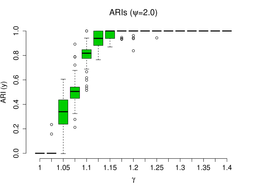
(a) Time clustering

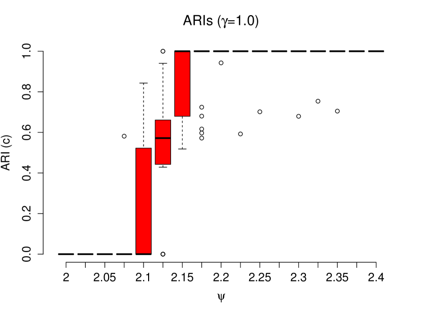
(b) Nodes clustering

Figure 1: Box plots of ARIs for both clusterings of nodes and time intervals. Both clusterings reach the maximum effectiveness for higher values of contrast parameters.

In Figure 1(a), we set $\psi=2$, which means there is not any community structure and let $\gamma$ varying in the range $[1,1.05,\dots,1.4]$. Adjusted Rand Indexes (ARIs) [34] are used to assess the time clustering, varying between zero (null clustering) and one (optimal clustering). When $\gamma=1$ we are in a degenerate case and no time structure affects the interactions: not surprisingly the algorithm assigns all the intervals to the same cluster (null ARI). The higher the value of $\gamma$ the more effective the clustering is up to a perfect recovery of the planted structure (ARI of 1). In particular the true time structure is fully recovered for all the fifty graphs when $\gamma$ is higher than $1.3$.

Similar results can be observed in Figure 1(b) about nodes clustering: by setting $\gamma=1$, we removed any time structure and a stationary community structure is detected by the model. In this case it is interesting to make a comparison with a traditional SBM, which is expected to give similar results to those shown in Figure 1(b). For a fixed value of $\psi$ we simulated a dynamic graph, corresponding to 50 adjacency matrices, one per time interval. Then a static graph is obtained by summing up these adjacency matrices. The temporal SBM (TSBM) we propose deals with the dynamic graph, whereas a SBM is used on the static graph . The Gibbs sampling algorithm introduced in [35] was used to recover the number of clusters and cluster memberships according to a SBM (with Poisson distributed edge values). The experiment was repeated 50 times for each value of $\psi$ in the set $\{2.15,2.35,2.55\}$. In Figure 2 we compare the ARIs of the two models for each value of $\psi$.

The greedy ICL TSBM (faster than the Gibbs sampling algorithm, who has an average runtime of 15.15 seconds) recovers the true structure at levels of contrast lower than those required by the Gibbs sampling algorithm (SBM). This comparison aims at showing that, in a stationary framework, the TSBM works at least as well as a standard SBM. The difference in terms of performance of the two models in this context can certainly be explained by the greedy search approach which is more effective than Gibbs sampling, as expected (see [16] and section 1).

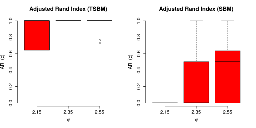
Figure 2: Comparison between the temporal SBM we propose and a classical SBM in a stationary context (any time cluster).

4.1.2 Optimization strategies

As mentioned in the previous section, in the present experiments, the optimization strategy A is more efficient than the two other strategies outlined in Section 3.4. We illustrate this superiority in the following test: the pair $(\gamma,\psi)$ is set to $(1,2.15)$ and 50 dynamic graphs are simulated according to the same settings discussed so far. Three different estimations are obtained, one for each strategy, and ARIs for nodes labels are computed. Results in Figure (3) can be compared with the mean value of the final ICL for each strategy:

	mean ICL
strategy A	$-70845.64$
strategy B	$-70894.67$
strategy C	$-70885.22$

4.1.3 Scalability

A full scalability analysis of the proposed algorithm is out of the scope of this paper (see B), but we have performed a limited assessment in this direction with a simple example.

A fixed $\gamma=1$ is maintained and for several values of $\psi$ and $50$ dynamic graphs with 100 nodes and 100 times intervals were sampled according to the intensity in equation (15). The mean runtime for reading and providing labels estimates for $each$ dynamic graph is 13.16 seconds. As expected, the algorithm needs a lower contrast to recover the true structure as the reader can observe by comparing Figure (4) with Figure (1(b)). This is a consequence of the increase in the number of interactions (induced by the longer time frame).

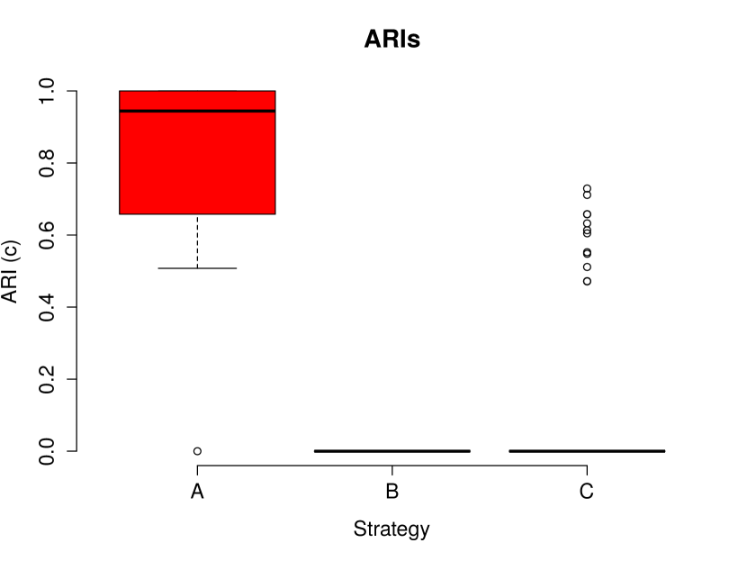
Figure 3: Box plots of 50 ARIs for clustering of nodes for each optimization strategy in the first scenario with $\psi=2.15$.

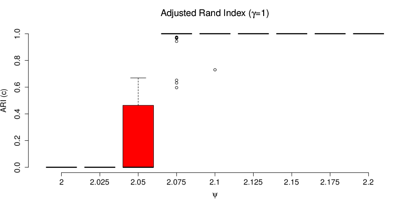
Figure 4: Box plots of 50 ARIs for clustering of nodes in the first scenario, with $N=100$ and $U=100$.

In terms of computational burden, each dynamic graph is handled in a average time of 13.16 seconds, that is less than 14 slower than in the case of a graph with 50 nodes and 50 time intervals. As we use $K_{max}=N/2$ and $D_{max}=U/2$, the worst case cost of one “iteration” of the algorithm is $O((N+U)UN^{2})$ and thus doubling both $N$ and $U$ should multiply the runtime by 16. On this limited example, the growth is slightly less than expected.

4.1.4 Non community structure

We now consider a different scenario showing how the TSBM model can perfectly recover a clustering structure in a situation where the SBM fails. We considered two clusters of nodes $A_{1}$ and $A_{2}$ and two time clusters $C_{1}$ and $C_{2}$ (clusters are balanced in average as in the previous examples). We simulated directed interactions between $50$ nodes over $100$ time intervals according to the following intensity matrix

$$\Lambda(u)=L_{1}\mathbf{1}_{C_{1}}(u)+L_{2}\mathbf{1}_{C_{2}}(u),\qquad u\in\{1,\dots,100\},$$ (16)

where

$$L_{1}=\begin{pmatrix}2&1\\ 1&2\\ \end{pmatrix}\qquad\text{and}\qquad L_{2}=\begin{pmatrix}1&2\\ 2&1\\ \end{pmatrix}.$$

In this scenario, a clustering structure is persistent over time, but the agents behaviour changes abruptly depending on the time cluster the interactions are taking place, moving from a community like pattern to a bipartite like one. When aggregating observations, since the expected percentage of time intervals belonging to cluster $C_{1}$ is $50\%$, the two opposite effects compensate each other (on average) and the SBM cannot detect any community structure. This can be seen in Figure 5: we simulated 50 dynamic graphs according to the Poisson intensities in equation (16) and estimates of $\mathbf{c}$ and $K$ are provided for each graph by both TSBM and SBM. The outliers ARIs in the right hand side figure (7 over 50) correspond to sampled vectors $\mathbf{y}$ in which the proportion of time intervals belonging to cluster $C_{1}$ is far from $1/2$. No outlier is observed when the experiment is performed with a fixed label vector $\mathbf{y}$ placing the same number of time intervals in each cluster.

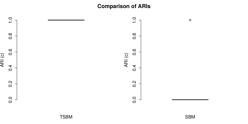
Figure 5: Comparison between the temporal SBM and a SBM in the second scenario.

The optimization strategy A has been used to produce the results shown in Figure 3. Very similar results can be obtained through optimization strategies B and C: with these settings the greedy ICL algorithm can always estimate the true vectors $\mathbf{c}$ and $\mathbf{y}$.

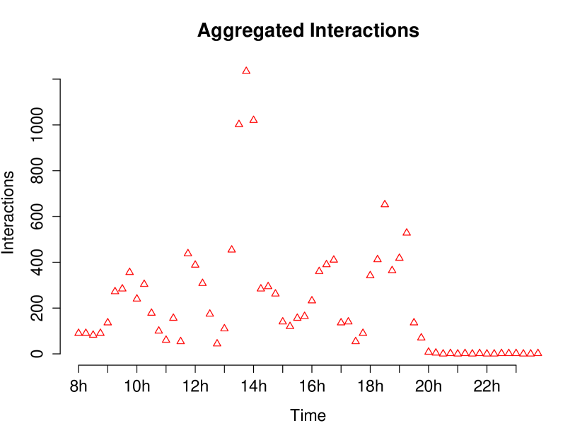
(a) Aggregated connections.

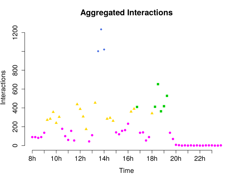
(b) Clustered time intervals.

Figure 6: Aggregated connections for each time interval (6(a)) and time clusters found by our model (6(b)) are compared.

4.2 Real Data

The data set we used was collected during the ACM Hypertext conference held in Turin, June 29th - July 1st, 2009. It represents the dynamic network of face-to-face proximity interactions of 113 conference attendees over about 2.5 days

We focused on the first conference day, namely the twenty four hours going from 8am of June 29th to 7.59am of June 30th. The day was partitioned in small time intervals of 20 seconds in the original data frame and interactions of face-to-face proximity (less than 1.5 meters) were monitored by electronic badges that attendees volunteered to wear. Further details can be found in [36]. We considered 15 minutes time aggregations, thus leading to a partition of the day made of 96 consecutive quarter-hours ($U=96$ with previous notation). A typical row of the aggregated data set looks like the following one:

ID$1$	ID$2$	Time Interval ($15m$)	Number of interactions
52	26	5	16

It means that conference attendees 52 and 26, between 9am and 9.15am, have spoken for $16\times 20s\approx 5m30s$.

In Figure 6(a), we computed the total number of interactions for each quarter hour. The presence of a time pattern is clear: the volume of interactions, for example, is much higher at $14$pm than at $9$am. The greedy ICL algorithm found 20 clusters for nodes (people) and 4 time clusters. Figure 6(b) shows how daily quarter-hours are assigned to each cluster: it can clearly be seen how time intervals corresponding to the highest number of interactions have been placed in cluster $C_{4}$, those corresponding to an intermediate interaction intensity, in $C_{2}$ (yellow) and $C_{3}$ (green). Cluster $C_{1}$ (magenta) contains intervals marked by a weaker intensity of interactions. It is interesting to note how the model closely recovers times of social gathering:

• 9.00-10.30 - set-up time for posters and demos.

• 13.00-15.00 - lunch break.

• 18.00-19.00 - wine and cheese reception.

Results in Figure 6 are obtained through the optimization strategy A. To make a comparison with the other two optimization strategies, we run the algorithm ten times for each strategy (A, B and C) and compare the final values of the ICL. Labels $\mathbf{c}$ and $\mathbf{y}$ are randomly initialized before each run, according to multinomial distributions (no hierarchical clustering was used) and $K_{\max}$ and $D_{\max}$ are set equal to $N/2$ and $U/2$, respectively. The mean final values of the ICL are reported in the following table:

	mean ICL
Strategy A	$-32746.51$
Strategy B	$-33072.99$
Strategy C	$-32116.01$

As it can be seen, the hybrid strategy C is the one leading to the highest final ICL, on average. In Figure (7) we report the final value of the ICL for each run (from 1 to 10) for each strategy. The optimization strategy C always outperforms the remaining two patterns.

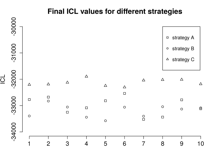
Figure 7: Comparison between the final values of the ICL obtained through different optimization strategies. On the horizontal axis we have the index of the experiment, on the vertical axis the final value of the ICL for each strategy.

5 Conclusion

We proposed a non-stationary extension of the stochastic block model (SBM) allowing us to simultaneously cluster nodes and infer the time structure of a network. The approach we chose consists in partitioning the time interval over which interactions are studied into sub-interval of fixed identical duration. Those intervals provide aggregated interaction counts that are studied with a SBM inspired model: nodes and time intervals are clustered in such a way that aggregated interaction counts are homogeneous over clusters. We derived an exact integrated classification likelihood (ICL) for such a model and proposed to maximize it with a greedy search strategy. The experiments we run on artificial and real world networks highlight the capacity of the model to capture non-stationary structures in dynamic graphs.

Appendix A Joint integrated density for labels

Consider at first the vector $\mathbf{c}$, whose joint probability function is given by (1). We attach a Dirichlet a priori distribution to the $K$-vector $\boldsymbol{\omega}$

$$p(\boldsymbol{\omega}|\alpha,K)=\frac{\Gamma(\alpha K)}{\Gamma(\alpha)^{K}}\prod_{k=1}^{K}\omega_{k}^{\alpha-1}.$$

The joint probability density for the pair $(\mathbf{c,\boldsymbol{\omega}})$ is obtained by multiplying (1) by the prior density

$$p(\mathbf{c},\boldsymbol{\omega}|\alpha,K)=\frac{\Gamma(\alpha K)}{\Gamma(\alpha)^{K}}\prod_{k=1}^{K}\omega_{k}^{|A_{k}|+\alpha-1}.$$

This is still a Dirichlet probability density function of parameters ($|A_{1}|+\alpha,\dots,|A_{K}|+\alpha$) and integration with respect to $\boldsymbol{\omega}$ is straightforward

$$p(\mathbf{c}|\alpha,K)= \frac{\Gamma(\alpha K)}{\Gamma(\alpha)^{K}}\int_{\boldsymbol{\omega}}\prod_{k=1}^{K}\omega_{k}^{|A_{k}|+\alpha-1}d\boldsymbol{\omega},$$

$$= \frac{\Gamma(\alpha K)}{\Gamma(\alpha)^{K}}\frac{\prod_{k\leq K}\Gamma(|A_{k}|+\alpha)}{\Gamma(\sum_{k=1}^{K}(|A_{k}|+\alpha))}$$

$$\times\int_{\boldsymbol{\omega}}\text{Dir}(\boldsymbol{\omega};|A_{1}|+\alpha,\dots,|A_{K}|+\alpha)d\boldsymbol{\omega},$$

$$= \frac{\Gamma(\alpha K)}{\Gamma(\alpha)^{K}}\frac{\prod_{k\leq K}\Gamma(|A_{k}|+\alpha)}{\Gamma(N+\alpha K)}.$$

This integrated density corresponds to the first term on the right hand side of (12). The second term is obtained similarly and the joint density $p(\mathbf{c},\mathbf{y}|K,D)$ follows by independence.

Appendix B Computational complexity

To evaluate the computational complexity of the proposed algorithm, we assume that the gamma function can be computed in constant time (see [37]). The core computation task consists in evaluating the change in ICL induced by exchanges and merges. The main quantities involved in those computations are the $(L_{kgd})_{1\leq,k\leq g,1\leq d\leq D}$. We first describe how to handle those quantities and then analyze the cost of the exchange and merge operations.

B.1 Data structures

The quantities $(L_{kgd})_{1\leq,k\leq g,1\leq d\leq D}$ are stored in a three dimensional array that is never resized (it occupies a $O(K_{max}^{2}D_{max})$ memory space) so that at any time during the algorithm, accessing to a value or modifying it can be done in constant time. The quantities needed to compute $L_{kgd}$, the $S_{kgd}$, $P_{kgd}$ and $R_{kgd}$ are handled in a similar way.

In addition, we maintain aggregated interaction counts for each time interval and each node. More precisely, we have for instance for a time interval $I_{u}$

$$S_{kgu}:=\sum_{c_{i}=k}\sum_{c_{j}=g}N^{I_{u}}_{ij},$$

and similar quantities such as $P_{kgu}$. For a node $i$, we have e.g.

$$S_{igd}:=\sum_{c_{j}=g}\sum_{y_{u}=d}N^{I_{u}}_{ij},$$

and other related quantities. The memory occupied by those structures is in $O(N^{2}U)$. Cluster memberships and clusters sizes are also stored in arrays.

In order to evaluate the ICL change induced by an operation, we need to compute its effect on $L_{kgd}$ in order to obtain $L^{*}_{kgd}$. This can be done in constant time for one value. For instance moving time interval $I_{u}$ from $C_{d^{\prime}}$ to $C_{l}$ implies the following modifications:

• $S_{kgd^{\prime}}$ is reduced by $S_{kgu}$ while $S_{kgl}$ is increased by the same quantity;

• $P_{kgd^{\prime}}$ is divided by $P_{kgu}$ while $P_{kgl}$ is multiplied by the same quantity;

• $R_{kgd^{\prime}}$ is decreased by $|A_{k}||A_{g}|$ (or $|A_{k}|(|A_{k}|-1)$) while $R_{kgl}$ is increased by the same quantity.

When an exchange or a fusion is actually implemented, we update all the data structures. The update cost is dominated by the other phases of the algorithm. For instance when $I_{u}$ is moved from $d^{\prime}$ to $l$, we need to update:

• cluster memberships and cluster sizes, which is done in $O(1)$;

• $L_{kgd^{\prime}}$ and $L_{kgl}$ for all $k$ and $g$, which is done in $O(K^{2})$;

• aggregated counts and products, such as $S_{igd^{\prime}}$ and $S_{igl}$, which is done in $O(NKD)$.

Considering that $K\leq N$ and $D\leq U$, the total update cost is in $O(NKD)$ for time interval related operations and in $O(UK^{2})$ for node related operations.

B.2 Exchanges

The calculation of $\Delta^{E,T}_{d^{\prime}\rightarrow l}$ for a time interval cluster exchange from equation (13) involves a sum with $K^{2}$ terms. As explained above each term is obtained in constant time, thus the total computation time is in $O(K^{2})$. This has to be evaluated for all time clusters and for all time interval, summing to a total cost of $O(UDK^{2})$.

Similarly, the calculation of $\Delta^{E,V}_{d^{\prime}\rightarrow l}$ involves a fix number of sums with at most $KD$ terms in each sum. The total computation time is therefore in $O(KD)$. This had to be evaluated for each node and for all node clusters, summing to a total cost of $O(NK^{2}D)$.

Notice that we have evaluated the total cost of one exchange round, i.e., in the case where all time intervals (or all nodes) are considered once. This evaluation does not take into account the reduction in the number of clusters generally induced by exchanges.

B.3 Merges

Merges are very similar to exchange in terms of computational complexity. They involve comparable sums that can be computed efficiently using the data structures described above. The computational cost for one time cluster merge round is in $O(D^{2}K^{2})$ while it is in $O(K^{3}D)$ for node clusters.

B.4 Total cost

The worst case complexity of one full exchange phase (with each node and each time interval considered once) is $O((N+U)D_{max}K^{2}_{max})$. The worst case complexity of one merge with mixed GM is $O(D_{max}K^{2}_{max}(D_{max}+K_{max}))$ which is smaller than the previous one for $N\geq K_{max}$ and $U\geq D_{max}$. Thus the worst case complexity of one “iteration” of the algorithm is $O((N+U)D_{max}K^{2}_{max})$.

Unfortunately, the actual complexity of the algorithm, while obviously related to this quantity, is difficult to evaluate for two reasons. Firstly, we have no way to estimate the number of exchanges needed in the exchange phase (apart from bounding them with the number of possible partitions). Secondly, we observe in practice that exchanges reduce the number of clusters, especially when $D_{max}$ and $K_{max}$ are high (i.e. close to $U$ and $N$, respectively). Thus the actual cost of one individual exchange reduces very quickly during the first exchange phase leading to a vast overestimation of its cost using the proposed bounds. As a consequence, the merge phase is also quicker than evaluated by the bounds.

A practical evaluation of the behaviour of the algorithm, while outside the scope of this paper, would be very interesting to assess its potential use on large data sets.

References

References

- [1] J. Moreno, Who shall survive?: A new approach to the problem of human interrelations., Nervous and Mental Disease Publishing Co, 1934.
- [2] R. Albert, A. Barabási, Statistical mechanics of complex networks, Modern Physics 74 (2002) 47–97.
-
[3]
D. Snyder, E. L. Kick, Structural
position in the world system and economic growth, 1955-1970: A
multiple-network analysis of transnational interactions, American Journal of
Sociology 84 (5) (1979) pp. 1096–1126.
URL http://www.jstor.org/stable/2778218 - [4] A. Barabási, Z. Oltvai, Network biology: understanding the cell’s functional organization, Nature Rev. Genet 5 (2004) 101–113.
- [5] G. Palla, I. Derenyi, I. Farkas, T. Vicsek, Uncovering the overlapping community structure of complex networks in nature and society, Nature 435 (2005) 814–818.
- [6] N. Villa, F. Rossi, Q. Truong, Mining a medieval social network by kernel som and related methods, Arxiv preprint arXiv:0805.1374.
- [7] S. Fortunato, Community detection in graphs, Physics Reports 486 (3-5) (2010) 75 – 174.
- [8] M. Girvan, M. Newman, Community structure in social and biological networks, Proceedings of the National Academy of Sciences 99 (12) (2002) 7821.
- [9] P. Bickel, A. Chen, A nonparametric view of network models and newman–girvan and other modularities, Proceedings of the National Academy of Sciences 106 (50) (2009) 21068–21073.
- [10] P. Holland, K. Laskey, S. Leinhardt, Stochastic blockmodels: first steps, Social Networks 5 (1983) 109–137.
- [11] P. Latouche, E. Birmelé, C. Ambroise, Bayesian methods for graph clustering, Springer, 2009, pp. 229–239.
- [12] J.-J. Daudin, F. Picard, S. Robin, A mixture model for random graphs, Statistics and Computing 18 (2) (2008) 173–183.
- [13] P. Latouche, E. Birmelé, C. Ambroise, Variational bayesian inference and complexity control for stochastic block models, Statistical Modelling 12 (1) (2012) 93–115.
- [14] K. Nowicki, T. Snijders, Estimation and prediction for stochastic blockstructures, Journal of the American Statistical Association 96 (455) (2001) 1077–1087.
- [15] A. Mc Daid, T. Murphy, F. N., N. Hurley, Improved bayesian inference for the stochastic block model with application to large networks, Computational Statistics and Data Analysis 60 (2013) 12–31.
- [16] E. Côme, P. Latouche, Model selection and clustering in stochastic block models based on the exact integrated complete data likelihood, Statistical Modelling 15 (6) (2015) 564–589. doi:10.1177/1471082X15577017.
- [17] C. Kemp, J. Tenenbaum, T. Griffiths, T. Yamada, N. Ueda, Learning systems of concepts with an infinite relational model, in: Proceedings of the National Conference on Artificial Intelligence, Vol. 21, 2006, pp. 381–391.
- [18] A. Goldenberg, X. Zheng, S. E. Fienberg, E. M. Airoldi, A survey of statistical network models, Machine Learning 2 (2) (2009) 129–133. doi:10.1561/2200000005.
- [19] T. Yang, Y. Chi, S. Zhu, Y. Gong, R. Jin, Detecting communities and their evolutions in dynamic social networks – a bayesian approach, Machine learning 82 (2) (2011) 157–189.
- [20] K. S. Xu, A. O. Hero III, Dynamic stochastic blockmodels: Statistical models for time-evolving networks, in: Social Computing, Behavioral-Cultural Modeling and Prediction, Springer, 2013, pp. 201–210.
- [21] E. P. Xing, W. Fu, L. Song, A state-space mixed membership blockmodel for dynamic network tomography, Ann. Appl. Stat. 4 (2) (2010) 535–566. doi:10.1214/09-AOAS311.
- [22] C. Dubois, C. Butts, P. Smyth, Stochastic blockmodelling of relational event dynamics, in: International Conference on Artificial Intelligence and Statistics, Vol. 31 of the Journal of Machine Learning Research Proceedings, 2013, pp. 238–246.
- [23] R. Guigourès, M. Boullé, F. Rossi, A triclustering approach for time evolving graphs, in: Co-clustering and Applications, IEEE 12th International Conference on Data Mining Workshops (ICDMW 2012), Brussels, Belgium, 2012, pp. 115–122. doi:10.1109/ICDMW.2012.61.
-
[24]
R. Guigourès, M. Boullé, F. Rossi,
Discovering patterns in
time-varying graphs: a triclustering approach, Advances in Data Analysis and
Classification (2015) 1–28doi:10.1007/s11634-015-0218-6.
URL http://dx.doi.org/10.1007/s11634-015-0218-6 - [25] A. Randriamanamihaga, E. Côme, L. Oukhellou, G. Govaert, Clustering the vélib dynamic origin/destination flows using a family of poisson mixture models, Neurocomputing 141 (2014) 124–138.
- [26] J. Wyse, N. Friel, P. Latouche, Inferring structure in bipartite networks using the latent block model and exact icl, Network Science, to appear.
- [27] C. Matias, T. Rebafka, F. Villers, Estimation and clustering in a semiparametric Poisson process stochastic block model for longitudinal networks, ArXiv e-printsarXiv:1512.07075.
-
[28]
C. Matias, V. Miele,
Statistical clustering
of temporal networks through a dynamic stochastic block model, working
paper or preprint (Jun. 2015).
URL https://hal.archives-ouvertes.fr/hal-01167837 - [29] H. Akaike, A new look at the statistical model identification, IEEE Transactions on Automatic Control 19 (1974) 716–723.
- [30] G. Schwarz, Estimating the dimension of a model, Annals of Statistics 6 (1978) 461–464.
- [31] C. Biernacki, G. Celeux, G. Govaert, Assessing a mixture model for clustering with the integrated completed likelihood, Pattern Analysis and Machine Intelligence, IEEE Transactions on 22 (7) (2000) 719–725.
- [32] V. D. Blondel, J. loup Guillaume, R. Lambiotte, E. Lefebvre, Fast unfolding of communities in large networks (2008).
-
[33]
A. Noack, R. Rotta, Multi-level
algorithms for modularity clustering, CoRR abs/0812.4073.
URL http://arxiv.org/abs/0812.4073 - [34] W. M. Rand, Objective criteria for the evaluation of clustering methods, Journal of the American Statistical association 66 (336) (1971) 846–850.
- [35] L. Nouedoui, P. Latouche, Bayesian non parametric inference of discrete valued networks, in: 21-th European Symposium on Artificial Neural Networks, Computational Intelligence and Machine Learning (ESANN 2013), Bruges, Belgium, 2013, pp. 291–296.
- [36] L. Isella, J. Stehlé, A. Barrat, C. Cattuto, J. Pinton, W. Van den Broeck, What’s in a crowd? analysis of face-to-face behavioral networks, Journal of Theoretical Biology 271 (1) (2011) 166–180. doi:DOI:10.1016/j.jtbi.2010.11.033.
- [37] W. H. Press, S. A. Teukolsky, W. T. Vetterling, B. P. Flannery, Numerical Recipes 3rd Edition: The Art of Scientific Computing, 3rd Edition, Cambridge University Press, 2007.