Asymptotically optimal definite quadrature formulae of 4-th order

Abstract

We construct several sequences of asymptotically optimal definite quadrature formulae of fourth order and evaluate their error constants. Besides the asymptotical optimality, an advantage of our quadrature formulae is the explicit form of their weights and nodes. For the remainders of our quadrature formulae monotonicity properties are established when the integrand is a 4-convex function, and a-posteriori error estimates are proven.

1 Introduction

We study quadrature formulae of the form

$$Q_{n}[f]=\sum_{i=1}^{n}a_{i,n}\,f(\tau_{i,n})\,,\quad 0\leq\tau_{1,n}<\tau_{2,n}<\cdots<\tau_{n,n}\leq 1$$ (1)

for approximate evaluation of the definite integral

$$I[f]:=\int\limits_{0}^{1}f(x)\,dx\,.$$

Our interest is in definite quadrature formulae. Let us recall some definitions.

Definition 1

Quadrature formula (1) is said to be definite of order $r$, $\,r\in\mathbb{N}$, if there exists a real non-zero constant $c_{r}(Q_{n})$ such that its remainder functional admits the representation

$$R[Q_{n};f]:=I[f]-Q_{n}[f]=c_{r}(Q_{n})\,f^{(r)}(\xi)$$

for every $f\in C^{r}[0,1]$, with some $\xi\in[0,1]$ depending on $f$ .

Furthermore, $Q_{n}$ is called positive definite (resp., negative definite) of order $r$, if $c_{r}(Q_{n})>0$ ($c_{r}(Q_{n})<0$).

Obviously, if $Q_{n}$ is a definite quadrature formula of order $r$, then $Q_{n}$ has algebraic degree of precision $r-1$ (in short, $ADP(Q_{n})=r-1$), i.e., $R[Q_{n};f]=0$ whenever $f$ is an algebraic polynomial of degree at most $r-1$, and $R[Q_{n};x^{r}]\neq 0$.

Throughout this paper, by $r$-convex ($r$-concave) function $f$ we shall mean a function $f\in C^{r}[0,1]$ such that $f^{(r)}\geq 0$ ($f^{(r)}\leq 0$) on the interval $[0,1]$.

The importance of definite quadrature formulae of order $r$ lies in the one-sided approximation they provide for $I[f]$ when the integrand $f$ is $r$-convex (concave). If, e.g., $\{Q^{+},\ Q^{-}\}$ is a pair of a positive and a negative definite quadrature formula of order $r$ and $\,f\,$ is $r$-convex, then for the true value of $I[f]$ we have the inclusion $Q^{+}[f]\leq I[f]\leq Q^{-}[f]$. This simple observation serves as a base for derivation of a posteriori error estimates and rules for termination of calculations (stopping rules) in automatic numerical integration algorithms (see [5] for a survey). Most of quadratures used in practice (e.g., quadrature formulae of Gauss, Radau, Lobatto, Newton-Cotes) are definite of certain order.

Definite $n$-point quadrature formulae with smallest positive or largest negative error constant are called optimal definite quadrature formulae. Let us set

$$c_{n,r}^{+}:=\inf\{c_{n,r}(Q_{n})\,:\,Q_{n}\ \text{ is positive definite of order }\ r\}\,,$$

$$c_{n,r}^{-}:=\inf\{c_{n,r}(Q_{n})\,:\,Q_{n}\ \text{ is negative definite of order }\ r\}\,.$$

It should be pointed out that it is fairly not obvious that the above infimums are attained or that the optimal definite quadrature formulae are unique. The existence of optimal definite quadrature formulae was first proven by Schmeisser [16] for even $r$, and for arbitrary $r$ and more general boundary conditions by Jetter [7] and Lange [10]. The uniqueness has been proven by Lange [10, 11]. For even $r$, Lange [10] has shown that

$$\begin{split}&c_{n,r}^{+}=-\frac{B_{r}(j/2)}{n^{r}}\,\Big{(}1+O(n^{-1})\Big{)}\quad\text{ if }\ r=4m+2j\,,\\ &c_{n,r}^{-}=-\frac{B_{r}(j/2)}{n^{r}}\,\Big{(}1+O(n^{-1})\Big{)}\quad\text{ if }\ r=4m+2-2j\end{split}$$ (2)

for $j=1,\,2$, where $B_{r}$ is the $r$-th Bernoulli polynomial with leading coefficient $1/r!$ . Schmeisser [16] proved that the same result holds for optimal definite quadrature formulae with equidistant nodes.

The $n$-point optimal positive definite and the $(n+1)$-point optimal negative definite quadrature formulae of order $2$ are well-known: these are the $n$-th compound midpoint and trapezium quadrature formulae, respectively. The case $r=2$ is exceptional, as for $r\geq 3$ the optimal definite quadrature formulae are not known. Lange [10] has computed numerically, for $3\leq n\leq 30$, the $n$-point optimal definite quadrature formulae of order $3$ and the $n$-point optimal positive definite quadrature formulae of order $4$.

It is a general observation about the optimality concept in quadratures that, even though the existence and the uniqueness of the optimal quadrature formulae (for instance, in the non-periodic Sobolev classes of functions) is established, the optimal quadrature formulae remain unknown. This fact severely reduces the practical importance of optimal quadratures. The way out of this situation is to look for quadrature formulae which are nearly optimal, e.g., for sequences of asymptotically optimal quadrature formulae.

Definition 2

Let $\,\{Q_{n}\}_{n=n_{0}}^{\infty}$ be a sequence of positive (resp, negative) definite quadrature formulae of order $\,r$. $\,Q_{n}\,$ is said to be asymptotically optimal positive (negative) definite quadrature formula of order $r$, if

$$\lim_{n\rightarrow\infty}\frac{c_{r}(Q_{n})}{c_{n,r}^{+}}=1\qquad\text{resp., }\ \ \lim_{n\rightarrow\infty}\frac{c_{r}(Q_{n})}{c_{n,r}^{-}}=1\,.$$

In [16] Schmeisser proposed an approach for construction of asymptotically optimal definite quadrature formulae of even order $r$ with equidistant nodes. Köhler and Nikolov [9] have studied Gauss-type quadrature formulae associated with spaces of splines with double and equidistant knots, and as a result obtained bounds for the best constants $c_{n,r}^{+}$ and $c_{n,r}^{-}$. In particular, it has been shown in [9] that for even $r$ the corresponding Gauss-type quadrature formulae are asymptotically optimal definite quadrature formulae. Motivated by this result, in [14] Nikolov found explicit recurrence formulae for the evaluation of the nodes and the weights of the Gaussian formulae for the spaces of cubic splines with double equidistant knots, and proposed a numerical procedure for the construction of the Lobatto quadrature formulae for the same spaces of splines. According to [9], the Gauss and the Lobatto quadrature formulae for these spaces of splines are respectively asymptotically optimal positive definite and asymptotically optimal negative definite, of order $4$.

Although the evaluation of Gauss-type quadrature formulae for spaces of splines (also with single knots, because of their asymptotical optimality in certain Sobolev classes, see [8]) is highly desirable, there is a serious problem occurring already with the splines of degree $3$, and its difficulty increases with the splines degree: the mutual displacement of the nodes of the quadratures and the splines knots is unknown. For justifying the location of the quadrature abscissae with respect to the knots of the space of splines, additional assumptions are to be made. For instance, in a recent paper [1] Ait-Haddou, Bartoň and Calo extended the procedure from [14] for explicit evaluation of the Gaussian quadrature formulae for spaces of $C^{1}$ cubic splines with non-equidistant knots, assumming that the spline knots are symmetrically stretched. For another approach to the construction of Gaussian quadrature formulae for $C^{2}$ cubic splines via homotopy continuation, see [2].

In the present paper we construct several sequences of asymptotically optimal definite quadrature formulae of order $4$ with explicitly given nodes and weights. For their construction we make use of the Euler-Maclaurin summation formulae, associated with the midpoint and the trapezium quadrature formulae, replacing the values of the derivatives at the end-points by appropriate formulae for numerical differentiation (this idea is not new, it can be traced in the book of Brass [3], and, implicitly, has been applied already in [16]). Thus, our quadrature formulae differ from the compound midpoint or compound trapezium quadrature formula by very little: they have only few different weights and/or involve few additional nodes. We evaluate the error constants of our quadrature formulae, which, in view of their asymptotical optimality, are not essentially different. Our motivation for proposing not just two sequences of asymptotically optimal positive definite and negative definite quadrature formulae of order $4$ is that, when chosen appropriately, pairs of definite quadrature formulae of the same type furnish, similarly to the case of pairs of definite quadrature formulae of opposite type, error inclusions for $I[f]$ whenever the integrand $f$ is $4$-convex or $4$-concave.

The rest of the paper is organized as follows. Section 2 provides the necessary facts about Peano representation theorem for linear functionals, Bernoulli polynomials and Euler-Maclaurin summation formulae. In Section 3 we construct sequences of definite quadrature formulae of order $4$. In Section 4 we prove monotonicity of the remainders of some of our definite quadrature formulae under the assumption that the integrand is $4$-convex (concave), and as a result obtain a posteriori error estimates. Section 5 shows some numerical experiments, and Section 6 contains some final remarks.

2 Preliminaries

2.1 Peano kernel representation of linear functionals

Throughout the paper, $\pi_{m}$ will stand for the set of algebraic polynomials of degree not exceeding $m$.

By $W^{r}_{1}=W^{r}_{1}[0,1]$, $\,r\in\mathbb{N}$, we denote the Sobolev class of functions

$$W^{r}_{1}[0,1]:=\{f\in C^{r-1}[0,1]\,:\,f^{(r-1)}\mbox{ abs. continuous},\;\int_{0}^{1}\!|f^{(r)}(t)|\,dt<\infty\}\,.$$

In particular, we have $C^{r}[0,1]\subset W^{r}_{1}[0,1]$.

If ${\cal L}$ is a linear functional defined in $W^{r}_{1}[0,1]$ which vanishes on $\pi_{r-1}$, then, by a classical result of Peano [15], ${\cal L}$ admits the integral representation

$${\cal L}[f]=\int_{0}^{1}K_{r}(t)f^{(r)}(t)\,dt,\qquad\quad K_{r}(t)={\cal L}\Big{[}\frac{(\cdot-t)_{+}^{r-1}}{(r-1)!}\Big{]},\ \ t\in[0,1]\,,$$

where

$$u_{+}=\max\{u,0\}\,.$$

The function $K_{r}$ is called the $r$-th Peano kernel of ${\cal L}$. In the case when ${\cal L}$ is the remainder $R[Q_{n};\cdot]\,$ of the quadrature formula (1) and $ADP(Q_{n})\geq r-1$, $\,K_{r}(t)=K_{r}(Q_{n};t)\,$ is also referred to as the $r$-th Peano kernel of $Q_{n}$. An explicit representations of $\,K_{r}(Q_{n};t)\,$ for $t\in[0,1]$ is

$$K_{r}(Q_{n};t)=(-1)^{r}\Big{[}\frac{t^{r}}{r!}-\frac{1}{(r-1)!}\sum_{i=1}^{n}a_{i,n}(t-\tau_{i,n})_{+}^{r-1}\Big{]}.$$ (3)

$K_{r}(Q_{,};\cdot)$ is called also a monospline of degree $r$. From

$$R[Q_{n};f]=\int\limits_{0}^{1}K_{r}(Q_{n};t)\,f^{(r)}(t)\,dt$$ (4)

it is clear that $Q_{n}$ is a positive (negative) definite quadrature formula of order $r$ if and only if $ADP(Q_{n})=r-1$ and $K_{r}(Q_{n};t)\geq 0$ (resp., $K_{r}(Q_{n};t)\leq 0$) on $[0,1]$. For more details on the Peano kernel theory we refer to [3].

2.2 Bernoulli polynomials. Summation formulae of Euler–Maclaurin type

By appropriate integration by parts in (4) the remainder of a quadrature formula $Q_{n}$ with $ADP(Q_{n})=r-1\,$ can be further expanded in the form

$$R[Q_{n};f]=\sum_{\nu=r}^{s}C_{\nu}(0)\,\big{[}f^{(\nu-1)}(1)-f^{(\nu-1)}(0)\big{]}+\int\limits_{0}^{1}C_{s}(t)\,f^{(s)}(t)\,dt\,,$$ (5)

with some functions $\{C_{\nu}(x)\}$ depending on $Q_{n}$ (see [3] for details).

For the sake of convenience, let us fix some notations. For $n\in\mathbb{N}$, we set

$$x_{k,n}:=\frac{k}{n}\,,\quad(0\leq k\leq n)\,,\qquad y_{\ell,n}:=\frac{2\ell-1}{2n}\,,\quad(1\leq\ell\leq n)\,.$$ (6)

The $n$-th compound trapezium and midpoint quadrature formulae are denoted by $Q_{n}^{Tr}$ and $Q_{n}^{Mi}$, respectively, i.e.,

$$Q_{n}^{Tr}[f]:=\frac{1}{2n}\big{[}f(x_{0,n})+f(x_{n,n})\big{]}+\frac{1}{n}\,\sum_{k=1}^{n-1}f(x_{k,n})\,,\qquad Q_{n}^{Mi}[f]:=\frac{1}{n}\,\sum_{k=1}^{n}f(y_{k,n})\,.$$

The Bernoulli polynomials $B_{\nu}$ are defined recursively by

$$B_{0}(x)=1,\quad B_{\nu}^{\prime}(x)=B_{\nu-1}(x),\quad\ \int_{0}^{1}B_{\nu}(t)\,dt=0\,,\qquad\nu\in\mathbb{N}.$$

Here, we shall need the explicit form of $B_{4}(x)$, $B_{4}(x)=x^{2}(1-x)^{2}/24-1/720$, and shall exploit the fact that

$$-\frac{1}{720}=B_{4}(0)\leq B_{4}(x)\leq B_{4}(1/2)=\frac{7}{5760}\,,\qquad x\in[0,1]\,.$$ (7)

The $1$-periodic extension of $B_{\nu}(x)$ on $\mathbb{R}$ is denoted by $\widetilde{B}_{\nu}(x)$ and is called Bernoulli monospline. The expansion (5) with $\,Q_{n}=Q_{n}^{Mi}\,$ and $\,Q_{n}=Q_{n}^{Tr}\,$ yields the so-called Euler-Maclaurin summation formulae (see, e.g., [3, Satz 98, 99]). For easier further reference, they are given in a lemma:

Lemma 1

Assume that $f\in W^{s}_{1}$, where $s\in\mathbb{N},\ s\geq 2$. Then

$$R[Q_{n}^{Mi};f]\!=\!-\!\sum_{\nu=1}^{[\frac{s}{2}]}\!\frac{B_{2\nu}(1/2)}{n^{2\nu}}\big{[}f^{(2\nu\!-\!1)}(1)\!-\!f^{(2\nu\!-\!1)}(0)\big{]}\!+\!\frac{(-1)^{s}}{n^{s}}\!\int\limits_{0}^{1}\!\!\widetilde{B}_{s}\Big{(}nx-\frac{1}{2}\Big{)}f^{(s)}(x)dx$$

and

$$R[Q_{n}^{Tr};f]=-\!\sum_{\nu=1}^{[\frac{s}{2}]}\frac{B_{2\nu}(0)}{n^{2\nu}}\big{[}f^{(2\nu\!-\!1)}(1)\!-\!f^{(2\nu\!-\!1)}(0)\big{]}\!+\!\frac{(-1)^{s}}{n^{s}}\!\int\limits_{0}^{1}\!\widetilde{B}_{s}(nx)f^{(s)}(x)dx\,.$$

3 Asymptotically optimal definite quadrature formulae of $4$-th order

For verifying the asymptotical optimality of the definite quadrature formulae constructed in this section, we note that (2) with $r=4$ reads as

$$c_{n,4}^{+}=\frac{1}{720\,n^{4}}\,\Big{(}1+O(n^{-1})\Big{)}\,,\qquad c_{n,4}^{-}=-\frac{7}{5760\,n^{4}}\,\Big{(}1+O(n^{-1})\Big{)}\,.$$ (8)

Definition 3

For a given $\mathbf{t}=(t_{1},t_{2},t_{3},t_{4})$, $0\leq t_{1}<t_{2}<t_{3}<t_{4}<1/2$, we denote by $\,D_{1}(\mathbf{t})[f]\,$ and $\,D_{3}(\mathbf{t})[f]\,$ the interpolatory formulae for numerical differentiation with nodes $\{t_{i}\}_{i=1}^{4}$, which approximate $f^{\prime}(0)$ and $f^{\prime\prime\prime}(0)$, respectively. The formulae approximating $f^{\prime}(1)$ and $f^{\prime\prime\prime}(1)$ and obtained by reflection are denoted by $\,\widetilde{D}_{1}(\mathbf{t})[f]\,$ and $\,\widetilde{D}_{3}(\mathbf{t})[f]\,$, i.e.,

$$\widetilde{D}_{k}(\mathbf{t})[f]=D_{k}(\mathbf{t})[g]\,,\qquad g(x)=-f(1-x)\,,\quad k=1,3\,.$$

For the sake of brevity, we write $D(\mathbf{t})$ for the collection of four formulae for numerical differentiation $\{D_{1}[\mathbf{t}],\,\widetilde{D}_{1}(\mathbf{t}),\,D_{3}[\mathbf{t}],\,\widetilde{D}_{3}(\mathbf{t})\}$ .

3.1 Negative definite quadrature formulae of order $4$ based on $Q_{n}^{Tr}$

The second formula in Lemma 1 with $s=4$ can be rewritten in the form

$$\begin{split}\int\limits_{0}^{1}f(x)\,dx=&Q_{n}^{Tr}[f]-\frac{1}{12\,n^{2}}\big{[}f^{\prime}(1)-f^{\prime}(0)\big{]}+\frac{1}{384\,n^{4}}\big{[}f^{\prime\prime\prime}(1)-f^{\prime\prime\prime}(0)\big{]}\\ &+\frac{1}{n^{4}}\int\limits_{0}^{1}\big{[}\widetilde{B}_{4}(nx)-B_{4}(1/2)\big{]}\,f^{(4)}(x)\,dx\\ =:&Q_{n}^{\prime}[f]+\frac{1}{n^{4}}\int\limits_{0}^{1}\big{[}\widetilde{B}_{4}(nx)-B_{4}(1/2)\big{]}\,f^{(4)}(x)\,dx\,.\end{split}$$

Clearly, $Q_{n}^{\prime}$ is a negative definite quadrature formula of order $4$, since, in view of (7), $K_{4}(Q_{n}^{\prime};x)=n^{-4}\big{[}\widetilde{B}_{4}(nx)-B_{4}(1/2)\big{]}\leq 0$. However, $Q_{n}^{\prime}$ is not of the desired form, as it involves derivatives of the integrand. Therefore, we choose a set $D(\mathbf{t})$ of formulae for numerical differentiation to replace the values of $f^{\prime}$ and $f^{\prime\prime\prime}$ in $Q_{n}^{\prime}$, and thus to obtain a (symmetric) quadrature formula

$$Q=Q_{n}^{Tr}+\frac{1}{12\,n^{2}}\big{(}D_{1}(\mathbf{t})-\widetilde{D}_{1}(\mathbf{t})\big{)}-\frac{1}{384\,n^{4}}\big{(}D_{3}(\mathbf{t})-\widetilde{D}_{3}(\mathbf{t})\big{)}\,,$$ (9)

which involves at most $8$ nodes in addition to $\{x_{k,n}\}_{k=0}^{n}$. (In the sequel, we shall refer to $Q$ to as a quadrature formula generated by $D(\mathbf{t})$.) We have

$$R[Q;f]=R[Q_{n}^{\prime};f]+\frac{1}{12\,n^{2}}\,(L_{1}[f]-\widetilde{L}_{1}[f])-\frac{1}{384\,n^{4}}\,(L_{3}[f]-\widetilde{L}_{3}[f])\,,$$

where

$$L_{k}[f]:=f^{(k)}(0)-D_{k}(\mathbf{t})[f]\,,\quad\widetilde{L}_{k}[f]:=f^{(k)}(1)-\widetilde{D}_{k}(\mathbf{t})[f]\,,\qquad k=1,\,3\,.$$

The linear functionals $L_{k}$ and $\widetilde{L}_{k}$ vanish on $\pi_{3}$, hence $R[Q;f]$ vanishes on $f\in\pi_{3}$, too. From the definition of the Peano kernels it is readily seen that

$$K_{4}(L_{k};t)\equiv 0,\ \ t\in(t_{4},1]\,,\qquad K_{4}(\widetilde{L}_{k};t)\equiv 0,\ \ t\in[0,1-t_{4})\,,\quad k=1,\,3\,.$$

This implies the following important observation:

Proposition 1

The fourth Peano kernel of the symmetric quadrature formula $Q$ generated by $D(\mathbf{t})$ through (9) satisfies

$$K_{4}(Q;x)\equiv\frac{1}{n^{4}}\,\big{[}\widetilde{B}_{4}(nx)-B_{4}(1/2)\big{]},\qquad x\in[t_{4},1-t_{4}]\,.$$

As a consequence, $\,Q\,$ is negative definite of order $4$ if and only if $\,K_{4}(Q;x)\leq 0\,$ for $\,x\in(0,t_{4})$ .

It should be pointed out that not every set $D(\mathbf{t})$ of formulae for numerical differentiation generates a definite quadrature formula of order $4$.

Our first application of the above approach reveals a known result.

3.1.1 A quadrature formula of G. Schmeisser

The following $(n+1)$-point (with $n\geq 7$) asymptotically optimal negative definite quadrature formula of order $4$ was obtained in [16, eqn. (43)]:

$$\begin{split}Q_{n+1}[f]=&\frac{403}{1152n}\big{[}f(x_{0,n})\!+\!f(x_{n,n})\big{]}\!+\!\frac{159}{128n}\big{[}f(x_{1,n})\!+\!f(x_{n-1,n})\big{]}\\ &\!+\!\frac{113}{128n}\big{[}f(x_{2,n})\!+\!f(x_{n-2,n})\big{]}\!+\!\frac{1181}{1152n}\big{[}f(x_{3,n})\!+\!f(x_{n-3,n})\big{]}\!+\!\frac{1}{n}\sum_{k=4}^{n-4}f(x_{k,n})\,,\end{split}$$

with an error constant

$$c_{4}(Q_{n+1})=-\frac{7}{5760\,n^{4}}\Big{(}1+\frac{195}{7n}\Big{)}\,.$$

Schmeisser’s quadrature formula is generated by $D(x_{0,n},x_{1,n},x_{2,n},x_{3,n})$. As this is a known result, we do not enter into details.

3.1.2 A quadrature formula generated by $D(x_{0,n},x_{1,3n},x_{2,3n},x_{1,n})$

For $\mathbf{t}=(x_{0,n},x_{1,3n},x_{2,3n},x_{1,n})$ we have

$$D_{1}(\mathbf{t})[f]=\frac{n}{2}\big{[}-11f(x_{0,n})+18f(x_{1,3n})-9f(x_{2,3n})+2f(x_{1,n})\big{]}\,,$$

$$D_{3}(\mathbf{t})[f]=27\,n^{3}\big{[}-f(x_{0,n})+3f(x_{1,3n})-3f(x_{2,3n})+f(x_{1,n})\big{]}\,,$$

and $\,\widetilde{D}_{1}(\mathbf{t})$, $\,\widetilde{D}_{1}(\mathbf{t})\,$ are obtained from $D_{1}(\mathbf{t})$ and $D_{3}(\mathbf{t})$ by reflection. By (9) $D(\mathbf{t})$ generates a symmetric $(n+5)$-point quadrature formula

$$Q_{n+5}[f]=\sum_{k=1}^{n+5}A_{k,n+5}f(\tau_{k,n})\,,$$

with nodes $\{\tau_{i,n+5}\}_{i=1}^{n+5}$ given by

$$\begin{array}[]{l}\tau_{k,n+5}=x_{k-1,3n},\ 1\leq k\leq 3\vspace*{1mm}\\ \tau_{k,n+5}=x_{k-3,n},\ \ 4\leq k\leq n+2\vspace*{1mm}\\ \tau_{k,n+5}=x_{2n-5+k,3n},\ n+3\leq k\leq n+5\,,\end{array}$$

and weights

$$\begin{array}[]{ll}A_{1,n+5}=A_{n+5,n+5}=\frac{43}{384n},&A_{2,n+5}=A_{n+4,n+5}=\frac{69}{128n},\vspace*{2mm}\\ A_{3,n+5}=A_{n+3,n+5}=-\frac{21}{128n},&A_{4,n+5}=A_{n+2,n+5}=\frac{389}{384n},\vspace*{2mm}\\ A_{k,n+5}=\frac{1}{n},\ 5\leq k\leq n+1\,.&\end{array}$$

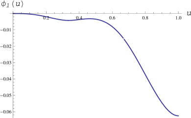
Figure 1: Graphs of $\,\phi_{1}(u)\,$ (left), and $\,K_{4}(Q_{n+5};t)$, $n=10\;$ (right).

In view of Proposition (1), to verify that $Q_{n+5}$ is a negative definite quadrature formula of order $4$, we only have to show that $\,K_{4}(Q_{n+5};t)<0\,$ for $\,t\in(0,x_{1,n})$. By substituting $t=u/n$, $\,u\in(0,1)$, this task reduces to

$$\phi_{1}(u):=u^{4}-\frac{43}{96}\,u^{3}-\frac{69}{32}\,(u-1/3)_{+}^{3}+\frac{21}{32}\,(u-2/3)_{+}^{3}\stackrel{{\scriptstyle?}}{{\leq}}0\,,\qquad u\in(0,1)\,.$$

The verification is straightforward, and we omit it. The graphs of $\phi_{1}(u)$ and $\,K_{4}(Q_{n+5};t)$, with $\,n=10$, are depicted on Figure 1.

For the evaluation of the error constant $c_{4}(Q_{n+5})=I[K_{4}(Q_{n+5};\cdot)]$, we make use of Proposition 1 and the fact that $K_{4}(Q_{n+5};\cdot)$ is symmetric, hence

$$\begin{split}c_{4}(Q_{n+5})&=2\int_{0}^{x_{1,n}}K_{4}(Q_{n+5};t)dt+\frac{1}{n^{4}}\int_{x_{1,n}}^{x_{n-1,n}}\big{[}\widetilde{B}_{4}(n\,t)-B_{4}(1/2)\big{]}dt\\ &=\frac{1}{12\,n^{5}}\int_{0}^{1}\phi_{1}(u)\,du-\frac{B_{4}(1/2)}{n^{4}}\Big{(}1-\frac{2}{n}\Big{)}\,.\end{split}$$

A further calculation shows that $I[\phi_{1}]=-71/4320$ and

$$c(Q_{n+5})=-\frac{7}{5760\,n^{4}}\Big{(}1-\frac{55}{63\,n}\Big{)}\,.$$

3.1.3 A quadrature formula generated by $D(x_{0,n},y_{1,n},x_{1,n},x_{2,n})$

With this set of formulae for numerical differentiation we get through (9) an $(n+3)$-point quadrature formula

$$Q_{n+3}[f]=\sum_{k=1}^{n+3}A_{k,n}f(\tau_{k,n+3})$$

with nodes

$$\begin{array}[]{llll}\tau_{1,n+3}=x_{0,n},&\tau_{2,n+3}=y_{1,n},&\tau_{n+2,n+3}=y_{n-1,n}&\tau_{n+3,n+3}=x_{n,n}\,,\vspace*{1mm}\\ \tau_{k,n+3}=x_{k-2,n},&3\leq k\leq n+1\,,&&\end{array}$$

and weights

$$\begin{array}[]{ll}A_{1,n+3}=A_{n+3,n+3}=\frac{43}{192n},&A_{2,n+3}=A_{n+2,n+3}=\frac{29}{72n},\vspace*{2mm}\\ A_{3,n+3}=A_{n+1,n+3}=\frac{83}{96n},&A_{4,n+3}=A_{n,n+3}=\frac{581}{576n},\vspace*{2mm}\\ A_{k,n+3}=\frac{1}{n},\ 5\leq k\leq n-1\,.&\end{array}$$

In view of Proposition 1, $Q_{n+3}$ is a negative definite of order $4$ if and only if $\,K_{4}(Q_{n+3};t)<0\,$ for $\,t\in(0,x_{2,n})$. By change of variable $t=u/n$, $u\in(0,2)$, this condition becomes

$$\phi_{2}(u):=u^{4}-\frac{43}{48}\,u^{3}-\frac{29}{18}\,(u-1/2)_{+}^{3}-\frac{83}{24}\,(u-1)_{+}^{3}<0\,,\quad u\in(0,2)\,,$$

and it is not difficult to verify that it is fulfilled.

For the error constant $c_{4}(Q_{n+3})=I[K_{4}(Q_{n+3};\cdot)]$ we have

$$\begin{split}c_{4}(Q_{n+3})&=2\int_{0}^{x_{2,n}}K_{4}(Q_{n+3};t)dt+\frac{1}{n^{4}}\int_{x_{2,n}}^{x_{n-2,n}}\big{[}\widetilde{B}_{4}(n\,t)-B_{4}(1/2)\big{]}dt\\ &=\frac{1}{12\,n^{5}}\int_{0}^{2}\phi_{2}(u)\,du-\frac{B_{4}(1/2)}{n^{4}}\Big{(}1-\frac{4}{n}\Big{)}\,,\end{split}$$

and after evaluation of the integral of $\phi_{2}$, we obtain

$$c(Q_{n+3})=-\frac{7}{5760\,n^{4}}\Big{(}1+\frac{55}{28\,n}\Big{)}\,.$$

3.2 Negative definite quadrature formulae of order $4$ based on $Q_{n}^{Mi}$

We rewrite the first Euler-Maclaurin summation formula in Lemma 1 with $s=4$ in the form

$$\begin{split}\int\limits_{0}^{1}\!\!f(x)dx&\!=\!Q_{n}^{Mi}[f]\!+\!\frac{1}{24\,n^{2}}\big{[}f^{\prime}(1)\!-\!f^{\prime}(0)\big{]}\!+\!\frac{1}{n^{4}}\!\int\limits_{0}^{1}\!\!\big{[}\widetilde{B}_{4}(nx-\frac{1}{2})-B_{4}(\frac{1}{2})\big{]}\,f^{(4)}(x)dx\\ &\!=:Q_{n}^{\prime\prime}[f]+\frac{1}{n^{4}}\!\int\limits_{0}^{1}\!\!\big{[}\widetilde{B}_{4}(nx-\frac{1}{2})-B_{4}(\frac{1}{2})\big{]}\,f^{(4)}(x)dx\,.\end{split}$$

Here, $Q_{n}^{\prime\prime}$ is a negative definite quadrature formula of order $4$, as, by (7), its fourth Peano kernel $K_{4}(Q_{n}^{\prime\prime};x)=n^{-4}\big{[}\widetilde{B}_{4}(nx-1/2)-B_{4}(1/2)\big{]}\,$ is non-positive. Since $Q_{n}^{\prime\prime}$ is not of the desired form, we choose a set $D(\mathbf{t})$ of formulae for numerical differentiation to replace the values of $f^{\prime}$ in $Q_{n}^{\prime\prime}[f]$, and thus to obtain a (symmetric) quadrature formula

$$Q=Q_{n}^{Mi}-\frac{1}{12\,n^{2}}\big{(}D_{1}(\mathbf{t})-\widetilde{D}_{1}(\mathbf{t})\big{)}\,,$$ (10)

which involves at most $8$ nodes in addition to $\,\{y_{k,n}\}_{k=1}^{n}$. By the same argument that led us to Proposition 1, here we have

Proposition 2

The fourth Peano kernel of the symmetric quadrature formula $Q$ generated by $D(\mathbf{t})$ through (10) satisfies

$$K_{4}(Q;x)\equiv\frac{1}{n^{4}}\,\big{[}\widetilde{B}_{4}(nx-\frac{1}{2})-B_{4}(\frac{1}{2})\big{]}\,,\qquad x\in[t_{4},1-t_{4}]\,.$$

Consequently, $\,Q\,$ is negative definite of order $4$ if and only if $\,K_{4}(Q;x)\leq 0\,$ for $\,x\in(0,t_{4})$ .

3.2.1 A quadrature formula generated by $D(x_{0,n},y_{1,n},y_{2,2n},x_{1,n})$

For $\,\mathbf{t}=(x_{0,n},y_{1,n},y_{2,2n},x_{1,n})\,$ we have

$$D_{1}(\mathbf{t})[f]=\frac{n}{3}\bigg{[}-13f(x_{0,n})+36f(y_{1,n})-32f(x_{3,4n})+9f(x_{1,n})\bigg{]},$$

and $D(\mathbf{t})$ generates through (10) a $(n+6)$-point quadrature formula

$$Q_{n+6}[f]=\sum_{k=1}^{n+6}A_{k,n+6}\,f(\tau_{k,n+6})$$

with nodes

$$\begin{array}[]{l}\tau_{1,n+6}=x_{0,n},\ \ \tau_{2,n+6}=y_{1,n},\ \ \tau_{3,n+6}=y_{2,2n},\ \ \tau_{4,n+6}=x_{1,n},\vspace*{1mm}\\ \tau_{k,n+6}=y_{k-3,n},\ \ \ \ \ 5\leq k\leq n+2,\vspace*{1mm}\\ \tau_{n+7-k,n+6}=1-\tau_{k,n+6},\ \ \ \ 1\leq k\leq 4\end{array}$$

and weights

$$\begin{array}[]{ll}A_{1,n+6}=A_{n+6,n+6}=\frac{13}{72n},&A_{2,n+6}=A_{n+5,n+6}=\frac{1}{2n},\vspace*{2mm}\\ A_{3,n+6}=A_{n+4,n+6}=\frac{4}{9n},&A_{4,n+6}=A_{n+3,n+6}=-\frac{1}{8n},\vspace*{2mm}\\ A_{k,n+6}=\frac{1}{n},\ \ \ 5\leq k\leq n+2\,.&\end{array}$$

By Proposition 2, to verify that $Q_{n+6}$ is a negative definite quadrature formula of order $4$, we only need to check whether $\,K_{4}(Q_{n+6};t)<0,\,$ $\,t\in(0,x_{1,n})$, which, after the change of variable $t=u/n$, becomes

$$\phi_{3}(u):=u^{4}-\frac{13}{18}\,u^{3}-2\,(u-1/2)_{+}^{3}-\frac{16}{9}\,(u-3/4)_{+}^{3}\stackrel{{\scriptstyle?}}{{\leq}}0\,,\quad u\in(0,1)\,.$$

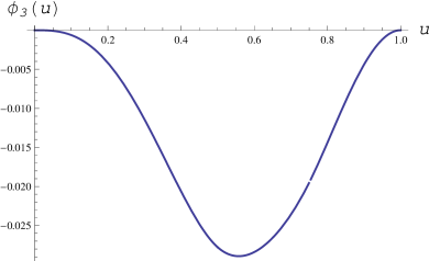
Figure 2: Graphs of $\,\phi_{3}(u)\,$ (left), and $\,K_{4}(Q_{n+6};t)$, $\,n=10\;$ (right).

The latter condition is fulfilled, as is seen also on Fugure 2 (left). For the error constant $c_{4}(Q_{n+6})$, in view of Proposition 2, we have

$$\begin{split}c_{4}(Q_{n+6})&=2\int_{0}^{x_{1,n}}K_{4}(Q_{n+6};t)dt+\frac{1}{n^{4}}\int_{x_{1,n}}^{x_{n-1,n}}\big{[}\widetilde{B}_{4}(n\,t-1/2)-B_{4}(1/2)\big{]}dt\\ &=\frac{1}{12\,n^{5}}\int_{0}^{1}\phi_{3}(u)\,du-\frac{B_{4}(1/2)}{n^{4}}\Big{(}1-\frac{2}{n}\Big{)}\,.\end{split}$$

With further calculations we find $I[\phi_{3}]=-13/960$ and

$$c_{4}(Q_{n+6})=-\frac{7}{5760\,n^{4}}\Big{(}1-\frac{15}{14\,n}\Big{)}\,.$$

Below we give two further negative definite quadrature formulae generated through (10).

3.2.2 A quadrature formula generated by $D(x_{0,n},y_{1,2n},y_{1,n},x_{1,n})$

For $t=(x_{0,n},y_{1,2n},y_{1,n},x_{1,n})$ we have

$$D_{1}(\mathbf{t})[f]=\frac{n}{3}\bigg{[}-21f(x_{0,n})+32f(y_{1,2n})-12f(y_{1,n})+f(x_{1,n})\bigg{]},$$

and $D(\mathbf{t})$ generates through (10) another $(n+6)$-point quadrature formula

$$Q_{n+6}[f]=\sum_{k=1}^{n+6}A_{k,n+6}\,f(\tau_{k,n+6})$$

with nodes

$$\begin{array}[]{l}\tau_{1,n+6}=x_{0,n},\ \ \tau_{2,n+6}=y_{1,2n},\ \ \tau_{3,n+6}=y_{1,n},\ \ \tau_{4,n+6}=x_{1,n},\vspace*{1mm}\\ \tau_{k,n+6}=y_{k-3,n},\ \ \ \ \ \ \ 5\leq k\leq n+2\,,\vspace*{1mm}\\ \tau_{n+7-k,n+6}=1-\tau_{k,n+6}\,,\vspace*{1mm}\ \ \ \ \ \ 1\leq k\leq 4\end{array}$$

and weights

$$\begin{array}[]{ll}A_{1,n+6}=A_{n+6,n+6}=\frac{7}{24n},&A_{2,n+6}=A_{n+5,n+6}=-\frac{4}{9n},\vspace*{2mm}\\ A_{3,n+6}=A_{n+4,n+6}=\frac{7}{6n},&A_{4,n+6}=A_{n+3,n+6}=-\frac{1}{72n},\vspace*{2mm}\\ A_{k,n+6}=\frac{1}{n},\ \ \ 5\leq k\leq n+2\,.&\end{array}$$

The error constant of $Q_{n+6}$ is

$$c_{4}(Q_{n+6})=-\frac{7}{5760\,n^{4}}\Big{(}1-\frac{5}{14\,n}\Big{)}\,.$$

3.2.3 A quadrature formula generated by $D(x_{0,n},y_{1,6n},y_{1,3n},y_{1,2n})$

With $\mathbf{t}=(x_{0,n},y_{1,6n},y_{1,3n},y_{1,2n})$, $\,D(\mathbf{t})$ generates a negative definite of order $4\,$ $\,(n+8)$-point quadrature formula

$$Q_{n+8}[f]=\sum_{k=1}^{n+8}A_{k,n+8}\,f(\tau_{k,n+8})$$

with nodes, weights and error constant given by

$$\begin{array}[]{l}\tau_{1,n+8}=x_{0,n},\ \ \tau_{2,n+8}=y_{1,6n},\ \ \tau_{3,n+8}=y_{1,3n},\ \ \tau_{4,n+8}=y_{1,2n},\vspace*{1mm}\\ \tau_{k,n+8}=y_{k-4,n},\ \ \ \ \ \ \ \ 5\leq k\leq n+4,\vspace*{1mm}\\ \tau_{n+9-k,n+8}=1-\tau_{k,n+8},\ \ \ \ \ \ \ 1\leq k\leq 4,\end{array}$$

$$\begin{array}[]{ll}A_{1,n+8}=A_{n+8,n+8}=\frac{11}{12n},&A_{2,n+8}=A_{n+7,n+8}=-\frac{3}{2n},\vspace*{2mm}\\ A_{3,n+8}=A_{n+6,n+8}=\frac{3}{4n},&A_{4,n+8}=A_{n+5,n+8}=-\frac{1}{6n},\vspace*{2mm}\\ A_{k,n+8}=\frac{1}{n},\ \ \ \ \ \ 5\leq k\leq n+4\,,&\end{array}$$

$$c_{4}(Q_{n+8})=-\frac{7}{5760\,n^{4}}\Big{(}1-\frac{5}{504\,n}\Big{)}\,.$$

Clearly, the error constant $c_{4}(Q_{n+8})$ is inferior to those of the preceding two quadrature formulae, which moreover involve two nodes less. The reason for quoting this quadrature formula will become clear in Section 4.

3.3 Positive definite quadrature formulae of order $4$ based on $Q_{n}^{Tr}$

We rewrite the second Euler-Maclaurin summation formula in Lemma 1 with $s=4$ in the form

$$\begin{split}\int\limits_{0}^{1}f(x)\,dx=&Q_{n}^{Tr}[f]-\frac{1}{12\,n^{2}}\big{[}f^{\prime}(1)-f^{\prime}(0)\big{]}+\frac{1}{n^{4}}\int\limits_{0}^{1}\big{[}\widetilde{B}_{4}(nx)-B_{4}(0)\big{]}\,f^{(4)}(x)\,dx\\ =:&\widetilde{Q}_{n}^{\prime}[f]+\frac{1}{n^{4}}\int\limits_{0}^{1}\big{[}\widetilde{B}_{4}(nx)-B_{4}(0)\big{]}\,f^{(4)}(x)\,dx\,.\end{split}$$

By (7), $\widetilde{Q}_{n}^{\prime}$ is a positive definite quadrature formula of order $4$, and we choose a set of formulae for numerical differentiation $D(\mathbf{t})$ to approximate $f^{\prime}(0)$ and $f^{\prime}(1)$ in $\widetilde{Q}_{n}^{\prime}$, thus arriving at a new quadrature formula

$$Q=Q_{n}^{Tr}+\frac{1}{12\,n^{2}}\,\big{(}D_{1}(\mathbf{t})-\widetilde{D}_{1}(\mathbf{t})\big{)}\,,$$ (11)

which involves at most $8$ nodes in addition to $\{x_{k,n}\}_{k=0}^{n}$ .

A statement analogous to Propositions 1, 2 holds true:

Proposition 3

The fourth Peano kernel of the symmetric quadrature formula $Q$ generated by $D(\mathbf{t})$ through (11) satisfies

$$K_{4}(Q;x)\equiv\frac{1}{n^{4}}\,\big{[}\widetilde{B}_{4}(nx)-B_{4}(0)\big{]}\,,\qquad x\in[t_{4},1-t_{4}]\,.$$

Consequently, $\,Q\,$ is positive definite of order $4$ if and only if $\,K_{4}(Q;x)\geq 0\,$ for $\,x\in(0,t_{4})$ .

Below we construct three positive definite quadrature formulae generated through (11) by different sets $D(\mathbf{t})$ of formulae for numerical differentiation.

3.3.1 A quadrature formula generated by $D(x_{0,n},y_{1,3n},x_{1,3n},y_{1,n})$

With $\mathbf{t}=(x_{0,n},y_{1,3n},x_{1,3n},y_{1,n})$, $D(\mathbf{t})$ generates through (11) an $(n+7)$-point symmetric quadrature formula

$$Q_{n+7}[f]=\sum_{k=1}^{n+7}A_{k,n+7}\,f(\tau_{k,n+7})$$

with nodes and weights given by

$$\begin{array}[]{l}\tau_{1,n+7}=x_{0,n},\ \ \tau_{2,n+7}=y_{1,3n},\ \ \tau_{3,n+7}=x_{1,3n},\ \ \tau_{4,n+7}=y_{1,n},\vspace*{1mm}\\ \tau_{k,n+7}=x_{k-4,n}\,,\ \ \ \ \ \ 5\leq k\leq n+3\,,\vspace*{1mm}\\ \tau_{n+8-k,n+7}=1-\tau_{k,n+7}\,,\ \ \ \ \ \ 1\leq k\leq 4\,,\end{array}$$

$$\begin{array}[]{ll}A_{1,n+7}=A_{n+7,n+7}=-\frac{5}{12n},&A_{2,n+7}=A_{n+6,n+7}=\frac{3}{2n},\vspace*{2mm}\\ A_{3,n+7}=A_{n+5,n+7}=-\frac{3}{4n},&A_{4,n+7}=A_{n+4,n+7}=\frac{1}{6n},\vspace*{2mm}\\ A_{k,n+7}=\frac{1}{n},\ \ \ 5\leq k\leq n+3\,.&\end{array}$$

By Proposition 3, the verification that $\,Q_{n+7}\,$ is positive definite of order $4$ reduces to $\,K_{4}(Q_{n+7};t)\geq 0\,$ for $\,t\in(0,y_{1,n})$, which, after the change of variable $t=u/n$, $u\in(0,1/2)$, becomes

$$\psi(u):=u^{4}+\frac{5}{3}\,u^{3}-6(u-1/6)_{+}^{3}+3(u-1/6)_{+}^{3}\stackrel{{\scriptstyle?}}{{\geq}}0\,,\quad u\in(0,1/2)\,.$$

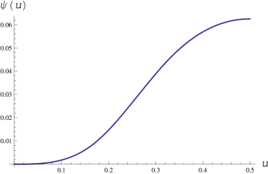
Figure 3: Graphs of $\,\psi(u)\,$ (left), and $\,K_{4}(Q_{n+7};t)$, $\,n=10\;$ (right).

The graph of $\psi$, depicted on Fugure 3 (left), shows that, indeed $\psi(u)>0$ for $u\in(0,1/2)$. Finally, in view of Proposition 3, for the error constant $c_{4}(Q_{n+7})$ we have

$$\begin{split}c_{4}(Q_{n+7})&=2\int_{0}^{y_{1,n}}K_{4}(Q_{n+6};t)dt+\frac{1}{n^{4}}\int_{y_{1,n}}^{y_{n-1,n}}\big{[}\widetilde{B}_{4}(n\,t)-B_{4}(0)\big{]}dt\\ &=\frac{1}{12\,n^{5}}\int_{0}^{1/2}\psi(u)\,du-\frac{B_{4}(0)}{n^{4}}\Big{(}1-\frac{1}{n}\Big{)}\,.\end{split}$$

The integral of $\psi$ is equal to $31/2160$, and a further simplification implies that

$$c_{4}(Q_{n+7})=\frac{1}{720\,n^{4}}\,\Big{(}1-\frac{5}{36\,n}\Big{)}.$$

The next two quadrature formulae are obtained through the same scheme. We only give their nodes, weights and error constants, skipping the details on the verification of their definiteness and the calculations, as these go along the same lines as in the case we just considered.

3.3.2 A quadrature formula generated by $D(x_{0,n},y_{1,2n},y_{1,n},x_{1,n})$

With $\mathbf{t}=(x_{0,n},y_{1,2n},y_{1,n},x_{1,n})$, $D(\mathbf{t})$ generates through (11) an $(n+5)$-point symmetric quadrature formula

$$Q_{n+5}[f]=\sum_{k=1}^{n+5}A_{k,n+5}\,f(\tau_{k,n+5})$$

with nodes and weights given by

$$\begin{array}[]{l}\tau_{1,n+5}=x_{0,n},\ \ \tau_{2,n+5}=y_{1,2n},\ \ \tau_{3,n+5}=y_{1,n},\ \ \tau_{4,n+5}=x_{1,n},\vspace*{1mm}\\ \tau_{k,n+5}=x_{k-3,n},\ \ \ \ \ \ \ 5\leq k\leq n+1,\vspace*{1mm}\\ \tau_{n+6-k,n+5}=1-\tau_{k,n+5},\ \ \ \ 1\leq k\leq 4\,,\end{array}$$

$$\begin{array}[]{ll}A_{1,n+5}=A_{n+5,n+5}=-\frac{1}{12n},&A_{2,n+5}=A_{n+4,n+5}=\frac{8}{9n},\vspace*{2mm}\\ A_{3,n+5}=A_{n+3,n+5}=-\frac{1}{3n},&A_{4,n+5}=A_{n+2,n+5}=\frac{37}{36n},\vspace*{2mm}\\ A_{k,n+5}=\frac{1}{n},\ \ \ \ \ \ \ 5\leq k\leq n+1\,.&\end{array}$$

The error constant of $Q_{n+5}$ is

$$c_{4}(Q_{n+5})=\frac{1}{720\,n^{4}}\,\Big{(}1-\frac{5}{8\,n}\Big{)}\,.$$

3.3.3 A quadrature formula generated by $D(x_{0,n},y_{1,2n},y_{1,n},y_{2,2n})$

With $\mathbf{t}=(x_{0,n},y_{1,2n},y_{1,n},y_{2,n})$, $D(\mathbf{t})$ generates through (11) an $(n+7)$-point symmetric quadrature formula

$$Q_{n+7}[f]=\sum_{k=1}^{n+7}A_{k,n+7}\,f(\tau_{k,n+7})$$

with nodes, weights and error constant given by

$$\begin{array}[]{l}\tau_{1,n+7}=x_{0,n},\ \ \tau_{2,n+7}=y_{1,2n},\ \ \tau_{3,n+7}=y_{1,n},\ \ \tau_{4,n+7}=y_{2,2n},\vspace*{1mm}\\ \tau_{k,n+7}=x_{k-4,n}\,,\ \ \ \ \ \ 5\leq k\leq n+3\,,\vspace*{1mm}\\ \tau_{n+8-k,n+7}=1-\tau_{k,n+7}\,,\ \ \ \ \ \ 1\leq k\leq 4\,,\end{array}$$

$$\begin{array}[]{ll}A_{1,n+7}=A_{n+7,n+7}=-\frac{1}{9n},&A_{2,n+7}=A_{n+6,n+7}=\frac{1}{n},\vspace*{2mm}\\ A_{3,n+7}=A_{n+5,n+7}=-\frac{1}{2n},&A_{4,n+7}=A_{n+4,n+7}=\frac{1}{9n},\vspace*{2mm}\\ A_{k,n+7}=\frac{1}{n},\ \ \ 5\leq k\leq n+3\,,&\end{array}$$

$$c_{4}(Q_{n+7})=\frac{1}{720\,n^{4}}\,\Big{(}1-\frac{15}{32\,n}\Big{)}.$$

3.4 Positive definite quadrature formulae of order $4$ based on $Q_{n}^{Mi}$

We write the first formula in Lemma 1 with $s=4$ in the form

$$\begin{split}\int\limits_{0}^{1}f(x)\,dx=&Q_{n}^{Mi}[f]+\frac{1}{24\,n^{2}}\big{[}f^{\prime}(1)-f^{\prime}(0)\big{]}-\frac{1}{384\,n^{4}}\big{[}f^{\prime\prime\prime}(1)-f^{\prime\prime\prime}(0)\big{]}\\ &+\frac{1}{n^{4}}\int\limits_{0}^{1}\Big{[}\widetilde{B}_{4}\Big{(}nx-\frac{1}{2}\Big{)}-B_{4}(0)\Big{]}\,f^{(4)}(x)\,dx\\ =:&\widetilde{Q}_{n}^{\prime\prime}[f]+\frac{1}{n^{4}}\int\limits_{0}^{1}\Big{[}\widetilde{B}_{4}\Big{(}nx-\frac{1}{2}\Big{)}-B_{4}(0)\Big{]}\,f^{(4)}(x)\,dx\,.\end{split}$$

We choose a set $D(\mathbf{t})$ for approximating the derivatives values in $\widetilde{Q}_{n}^{\prime\prime}$, thus obtaining a quadrature formula

$$Q=Q_{n}^{Mi}-\frac{1}{24\,n^{2}}\big{(}D_{1}(\mathbf{t})-\widetilde{D}_{1}(\mathbf{t})\big{)}+\frac{1}{384\,n^{4}}\big{(}D_{3}(\mathbf{t})-\widetilde{D}_{3}(\mathbf{t})\big{)}\,,$$ (12)

which involves at most $8$ nodes in addition to $\{y_{i,n}\}_{i=1}^{n}$. We have

Proposition 4

The fourth Peano kernel of the symmetric quadrature formula $Q$ generated by $D(\mathbf{t})$ through (12) satisfies

$$K_{4}(Q;x)\equiv\frac{1}{n^{4}}\,\big{[}\widetilde{B}_{4}(nx-\frac{1}{2})-B_{4}(0)\big{]}\,,\qquad x\in[t_{4},1-t_{4}]\,.$$

Consequently, $\,Q\,$ is positive definite of order $4$ if and only if $\,K_{4}(Q;x)\geq 0\,$ for $\,x\in(0,t_{4})$ .

On using Proposition 4, we verify the definiteness and evaluate the error constant of $Q$. We give below two positive definite quadrature formulae of order $4$, constructed on the basis of (12). As the definiteness verification and the evaluation of the error constants are completely analogous to that in the preceding cases, they are skipped here.

3.4.1 A quadrature formula generated by $D(y_{1,n},x_{1,n},y_{2,n},y_{3,n})$

With $\mathbf{t}=(y_{1,n},x_{1,n},y_{2,n},y_{3,n})$, $\,n\geq 7$, we obtain through (12) an $(n+2)$-point symmetric quadrature formula

$$Q_{n+2}[f]=\sum_{k=1}^{n+2}A_{k,n+2}\,f(\tau_{k,n+2})\,,$$

which is positive definite of order $4$. The nodes and the weights of $Q_{n+2}$ are

$$\begin{array}[]{l}\tau_{1,n+2}=y_{1,n},\ \ \tau_{2,n+2}=x_{1,n},\ \ \tau_{n+1,n+2}=x_{n-1,n},\ \ \tau_{n+2,n+2}=y_{n,n}\,,\vspace*{1mm}\\ \tau_{k,n+2}=y_{k-1,n},\ \ \ \ \ \ \ 3\leq k\leq n\,.\end{array}$$

$$\begin{array}[]{ll}A_{1,n+2}=A_{n+2,n+2}=\frac{251}{192n},&A_{2,n+2}=A_{n+1,n+2}=-\frac{43}{72n},\vspace*{2mm}\\ A_{3,n+2}=A_{n,n+2}=\frac{127}{96n},&A_{4,n+2}=A_{n-1,n+2}=\frac{557}{576n},\vspace*{2mm}\\ A_{k,n+2}=\frac{1}{n},\ \ \ \ \ \ \ 5\leq k\leq n-2\,.&\end{array}$$

The error constant of $Q_{n+2}$ is

$$c_{4}(Q_{n+2})=\frac{1}{720\,n^{4}}\,\Big{(}1+\frac{445}{32\,n}\Big{)}\,.$$

3.4.2 A quadrature formula generated by $D(x_{0,n},y_{1,3n},x_{1,3n},y_{1,n})$

With $\mathbf{t}=(x_{0,n},y_{1,3n},x_{1,3n},y_{1,n})$, $\,n\geq 3$, we obtain through (12) an $(n+6)$-point positive definite of order $4$ quadrature formula

$$Q_{n+6}[f]=\sum_{k=1}^{n+6}A_{k,n+6}\,f(\tau_{k,n+6})\,,$$

with nodes, weights and error constant given by

$$\begin{array}[]{l}\tau_{1,n+6}=x_{0,n},\ \ \tau_{2,n+6}=y_{1,3n},\ \ \tau_{3,n+6}=x_{1,3n},\ \ \tau_{4,n+6}=y_{1,n},\vspace*{1mm}\\ \tau_{k,n+6}=y_{k-3,n},\ \ \ \ \ \ \ \ \ \ 5\leq k\leq n+2,\vspace*{1mm}\\ \tau_{n+7-k,n+6}=\tau_{k,n+6},\ \ \ \ 1\leq k\leq 4\,,\end{array}$$

$$\begin{array}[]{ll}A_{1,n+6}=A_{n+6,n+6}=-\frac{5}{48n},&A_{2,n+6}=A_{n+5,n+6}=\frac{15}{16n},\vspace*{2mm}\\ A_{3,n+6}=A_{n+4,n+6}=-\frac{21}{16n},&A_{4,n+6}=A_{n+3,n+6}=\frac{71}{48n},\vspace*{2mm}\\ A_{k,n+6}=\frac{1}{n},\ \ \ \ \ \ \ 5\leq k\leq n+2\,,&\end{array}$$

$$c_{4}(Q_{n+6})=\frac{1}{720\,n^{4}}\,\Big{(}1-\frac{125}{144\,n}\Big{)}\,.$$

4 Monotonicity of the remainders and a posteriori error estimates

In this section we shall exploit the following general observation about definite quadrature formulae.

Theorem 1

Let $\,(Q^{\prime}\,,\,Q^{\prime\prime})\,$ be a pair of positive (negative) definite quadrature formulae of order $r$. Assume that, for some $c>0$, the quadrature formula

$$\widehat{Q}:=(c+1)\,Q^{\prime}-c\,Q^{\prime\prime}$$

is negative (positive) definite of order $r$. Then the following inequalities hold true whenever $\,f\,$ is an $\,r$-convex or $r$-concave function:

1. $\displaystyle{|R[Q^{\prime};f]|\leq\frac{c}{c+1}\,|R[Q^{\prime\prime};f]|}$ ;

2. $\displaystyle{|R[Q^{\prime};f]|\leq c\,|Q^{\prime}[f]-Q^{\prime\prime}[f]|}$ ;

3. $\displaystyle{|R[Q^{\prime\prime};f]|\leq(c+1)\,|Q^{\prime}[f]-Q^{\prime\prime}[f]|}$ .

Proof 1

Let us consider, e.g., the case when $Q^{\prime}$ and $Q^{\prime\prime}$ are negative definite and $\,\widehat{Q}\,$ is positive definite, of order $r$. Without loss of generality we may assume that $f$ is $r$-convex. Then $\,R[Q^{\prime};f]\leq 0$, $\,R[Q^{\prime\prime};f]\leq 0$, and $\,R[\widehat{Q};f]\geq 0$, therefore

$$0\leq R[\widehat{Q};f]=(c+1)\,R[Q^{\prime};f]-c\,R[Q^{\prime\prime};f]\,,$$

and hence

$$-R[Q^{\prime};f]\leq-\frac{c}{c+1}\,(R[Q^{\prime\prime};f])\,,$$

which, in this case, is exactly claim (i) of Theorem 1. Claim (iii) follows from

$$\begin{split}|Q^{\prime}[f]-Q^{\prime\prime}[f]|&=|R[Q^{\prime\prime};f]-R[Q^{\prime};f]|\geq|R[Q^{\prime\prime};f]|-|R[Q^{\prime};f]|\\ &\geq|R[Q^{\prime\prime};f]|-\frac{c}{c+1}\,|R[Q^{\prime\prime};f]|=\frac{1}{c+1}\,|R[Q^{\prime\prime};f]|\,,\end{split}$$

and (ii) is a consequence of (iii) and (i). The proof of the case when $Q^{\prime}$ and $Q^{\prime\prime}$ are positive definite and $\,\widehat{Q}\,$ is negative definite of order $r$ is analogous, and we omit it.

Remark 1

Notice the non-symmetric roles of $Q^{\prime}$ and $Q^{\prime\prime}$ in Theorem 1. Part (i) implies that for $r$-convex (concave) integrand $f$, $\,Q^{\prime}[f]\,$ furnishes a better approximation to $I[f]$ than $\,Q^{\prime\prime}[f]$. Another observation is that, the smaller $c>0$, the better a posteriori error estimates (ii) and (iii) we get. Hence, it makes sense to search for the best possible (i.e., the smallest) $\,c>0\,$ for which $\widehat{Q}$ is definite with the opposite type of definiteness to those of $Q^{\prime}$ and $Q^{\prime\prime}$.

Example 1

If $\,(Q^{\prime},Q_{n}^{\prime\prime})=(Q_{2n}^{Tr},Q_{n}^{Tr})$, then, since $\,\widehat{Q}=2Q_{2n}^{Tr}-Q_{n}^{Tr}=Q_{2n}^{Mi}\,$, the assumptions of Theorem 1 are fulfilled with $r=2$ and $c=1$. Hence, for $f$ convex, we have the (well-known) inequalities: $\displaystyle{|R[Q_{2n}^{Tr}[f]|\leq\frac{1}{2}\,|R[Q_{n}^{Tr}[f]|}$, $\,\displaystyle{|R[Q_{2n}^{Tr}[f]|\leq|Q_{n}^{Tr}[f]-Q_{2n}^{Tr}[f]|}$, and $\displaystyle{|R[Q_{n}^{Tr}[f]|\leq 2\,|Q_{n}^{Tr}[f]-Q_{2n}^{Tr}[f]|}$ .

Theorem 1 is applicable to some pairs of the definite quadrature formulae of order $4$, obtained in Section 3. In Tables 1 and 2 below, the notation $Q_{(3.b.c),m}$ stands for the quadrature, given in Section 3.b.c, with a parameter $n=m$.

Theorem 2

The assumptions of Theorem 1 are fulfilled for the pairs $\,(Q^{\prime},Q^{\prime\prime})\,$ of negative definite quadrature formulae and with the best possible constants $c$, given in Table 1.

No.	$Q^{\prime}$	$Q^{\prime\prime}$	$c$
$1$	$Q_{(3.2.1),2n}$	$Q_{(3.1.1),n}$	$\frac{104}{299}$
$2$	$Q_{(3.2.1),2n}$	$Q_{(3.1.3),n}$	$\frac{52}{77}$
$3$	$Q_{(3.2.1),2n}$	$Q_{(3.2.1),n}$	$1$
$4$	$Q_{(3.2.1),2n}$	$Q_{(3.2.2),n}$	$\frac{13}{29}$
$5$	$Q_{(3.2.1),2n}$	$Q_{(3.2.3),n}$	$\frac{1}{3}$
$6$	$Q_{(3.2.2),2n}$	$Q_{(3.1.1),n}$	$\frac{168}{235}$
$7$	$Q_{(3.2.2),2n}$	$Q_{(3.1.3),n}$	$\frac{28}{15}$
$8$	$Q_{(3.2.2),2n}$	$Q_{(3.2.2),n}$	$1$
$9$	$Q_{(3.2.2),2n}$	$Q_{(3.2.3),n}$	$\frac{1}{3}$
$10$	$Q_{(3.2.3),2n}$	$Q_{(3.2.3),n}$	$1$

Table 1: Pairs $(Q^{\prime},Q^{\prime\prime})$ of negative quadrature formulae of order $4$ and the corresponding best constants $c$, satisfying the assumptions of Theorem 1.

Proof 2

All we need is to check that $\widehat{Q}=(c+1)\,Q^{\prime}-c\,Q^{\prime\prime}\,$ is positive definite of order $4$. When studying $\,K_{4}(\widehat{Q};\cdot)\,$ in the neighborhoods of the endpoints of $[0,1]$, affected by the formulae for numerical differentiation applied to the construction of $\,Q^{\prime}\,$ and $\,Q^{\prime\prime}$, we eliminate the dependence on $n$ by a suitable change of the variable. Away from these neighborhoods we apply Propositions 1 – 2 to obtain a simpler representation of $\,K_{4}(\widehat{Q};\cdot)\,$. The verification that $\,K_{4}(\widehat{Q};\cdot)\,$ does not change its sign in $(0,1)$ consists of sometimes tedious though elementary calculations. We therefore decided to present a detailed proof of only one case, namely, case 9 in Table 1, and point out to some peculiarities in the other cases.

The interval unaffected by the formulae for numerical differentiation applied for the construction of $Q^{\prime}$ and $Q^{\prime\prime}$ in case 9 in Table 1, is $[y_{1,n},y_{n-1,n}]$. By Proposition 2, for $t\in[y_{1,n},y_{n-1,n}]$ we have

$$K_{4}(\widehat{Q};t)=\frac{c+1}{(2\,n)^{4}}\,\big{[}\widetilde{B}_{4}(2n\,t-\frac{1}{2})-B_{4}(1/2)\big{]}-\frac{c}{n^{4}}\,\big{[}\widetilde{B}_{4}(n\,t-\frac{1}{2})-B_{4}(1/2)\big{]}\,.$$

We shall show that

$$\varphi(t)=\varphi(c;t):=(c+1)\,\big{[}\widetilde{B}_{4}(2n\,t-1/2)-B_{4}(1/2)\big{]}-16c\,\big{[}\widetilde{B}_{4}(n\,t-1/2)-B_{4}(1/2)\big{]}$$

is non-negative for every $t\in\mathbb{R}$ if and only if $c\geq\frac{1}{3}$ . Since $\,\varphi\,$ is a periodic function with a period $1/n$, we study its behavior on the interval $\,[0,1/n]$ only.

Consider first the case $t\in[0,\frac{1}{4n}]\cup[\frac{3}{4n},\frac{1}{n}]$. If $\,t\in[0,\frac{1}{4n}]$, then we set $\,t=\frac{1-2u}{4n}\,$, while if $\,t\in[\frac{3}{4n},\frac{1}{n}]$, then we set $\,t=\frac{3+2u}{4n}\,$, with $\,u\in[0,\frac{1}{2}]$. In both cases we have $\,\widetilde{B}_{4}(2n\,t-1/2)=B_{4}(u)\,$ and $\,\widetilde{B}_{4}(n\,t-1/2)=B_{4}((2u+1)/4)$, therefore

$$\begin{split}\varphi(c;t)&=(c+1)\,\big{[}B_{4}(u)-B_{4}(1/2)\big{]}-16c\,\big{[}B_{4}((2u+1)/4)-B_{4}(1/2)\big{]}\\ &=\frac{(2u-1)^{2}}{64}\Big{[}c-\frac{1+4u(1-u)}{6}\Big{]}\,,\quad u\in[0,1/2]\,.\end{split}$$

The latter expression is non-negative for every $\,u\in[0,1/2]\,$ if and only if $c\geq 1/3$.

Next, we consider $\,\varphi(t)\,$ with $\,t\in[\frac{1}{4n},\frac{3}{4n}]$. For $\,t\in[\frac{1}{4n},\frac{1}{2n}]\,$ we set $\,t=\frac{1-u}{2n}$, while for $\,t\in[\frac{1}{2n},\frac{3}{4n}]\,$ we set $\,t=\frac{1+u}{2n}$, with $\,u\in[0,\frac{1}{2}]$. In both cases, we have $\,\widetilde{B}_{4}(2n\,t-1/2)=B_{4}(u+1/2)\,$ and $\,\widetilde{B}_{4}(n\,t-1/2)=B_{4}(u/2)$, therefore

$$\begin{split}\varphi(c;t)&=(c+1)\,\big{[}B_{4}(u+1/2)-B_{4}(1/2)\big{]}-16c\,\big{[}B_{4}(u/2)-B_{4}(1/2)\big{]}\\ &=\frac{c}{48}\,\big{(}8u^{3}-9u^{2}+2\big{)}-\frac{1}{48}\,u^{2}(1-2u^{2})\,,\quad u\in[0,1/2]\,.\end{split}$$

As $\varphi$ is an increasing function of $c$ and $\varphi(1/3;t)=(3u^{4}+4u^{3}-6u^{2}+1)/72>0$, $u\in[0,1/2]$, we conclude that $\varphi(t)\geq 0$ in that case, too, provided $c\geq 1/3$. Consequently, for $c\geq 1/3$ and $t\in[y_{1,n},y_{n-1,n}]$, $\,K_{4}(\widehat{Q};t)=(2n)^{-4}\,\varphi(c;t)\geq 0$.

Since $\,\widehat{Q}=(c+1)Q^{\prime}-c\,Q^{\prime\prime}\,$ is a symmetrical quadrature formula, it remains to verify (with $c=1/3$) that $\,K_{4}(\widehat{Q};t)\geq 0\,$ for $\,t\in[0,y_{1,n}]$. As similar verifications were repeatedly performed in the preceding section, here we omit the details.

Let us now briefly comment on the other pairs of quadratures in Table 1. The restriction on $c$ for the pairs of quadratures in lines $1-4$, $6-8$ and $10$ of Table 1 comes from the fact that a closed-type quadrature formula $\,\widehat{Q}\,$ can by positive definite of order $4$ only if the coefficient of $f(0)$ in $\,\widehat{Q}\,$ is non-negative, a fact that easily follows from the explicit form of $\,K_{4}(\widehat{Q};t)\,$, see (3). Actually, the values of $c$ in Table 1 in these cases are those, for which $\widehat{Q}$ is of open type; it turns out that these values of $c$ secure the positive definiteness of $\,\widehat{Q}\,$.

Theorem 3

The assumptions of Theorem 1 are fulfilled for the pairs $\,(Q^{\prime},Q^{\prime\prime})\,$ of positive definite quadrature formulae and with the best possible constants $c$, given in Table 2.

No.	$Q^{\prime}$	$Q^{\prime\prime}$	$c$
$1^{\prime}$	$Q_{(3.3.1),2n}$	$Q_{(3.3.1),n}$	$1.104931$
$2^{\prime}$	$Q_{(3.3.2),2n}$	$Q_{(3.3.1),n}$	$\frac{1}{3}$
$3^{\prime}$	$Q_{(3.3.2),2n}$	$Q_{(3.3.2),n}$	$1.803456$
$4^{\prime}$	$Q_{(3.3.2),2n}$	$Q_{(3.3.3),n}$	$1.088270$
$5^{\prime}$	$Q_{(3.3.2),2n}$	$Q_{(3.4.2),n}$	$1.207773$
$6^{\prime}$	$Q_{(3.3.3),2n}$	$Q_{(3.3.1),n}$	$\frac{1}{3}$
$7^{\prime}$	$Q_{(3.3.3),2n}$	$Q_{(3.3.3),n}$	$1.601589$
$8^{\prime}$	$Q_{(3.3.3),2n}$	$Q_{(3.4.2),n}$	$1.828256$

Table 2: Pairs $(Q^{\prime},Q^{\prime\prime})$ of positive definite quadrature formulae of order $4$ and the corresponding best constants $c$, satisfying the assumptions of Theorem 1.

Proof 3

We have to verify that $\widehat{Q}=(c+1)\,Q^{\prime}-c\,Q^{\prime\prime}\,$ is negative definite of order $4$. Two kinds of violation of the requirement $\,K_{4}(\widehat{Q};t)\leq 0\,$ may occur while decreasing $c$:

1. The requirement is first violated inside the neighborhoods of the endpoints of $[0,1]$, affected by the formulae for numerical differentiation applied to the construction of $\,Q^{\prime}\,$ and $\,Q^{\prime\prime}$. Then the best constant $c$ is a numerically computed zero of the resultant of a quintic polynomial, with which the corresponding (re-scaled) Peano kernels coincides.

2. The requirement is first violated away of these neighborhoods. There, we exploit Propositions 3 and 4 to obtain a simpler form of $\,K_{4}(\widehat{Q};\cdot)\,$. Such a situation occurs in the cases $2^{\prime}$ and $5^{\prime}$ in Table 2.

Here we consider in details only case $2^{\prime}$ in Table 2. The interval not affected by the formulae for numerical differentiation applied to the construction of $Q^{\prime}$ and $Q^{\prime\prime}$ is $[y_{1,n},y_{n-1,n}]$. By Proposition 3, for $t\in[y_{1,n},y_{n-1,n}]$ we have

$$K_{4}(\widehat{Q};t)=\frac{c+1}{(2n)^{4}}\,\big{[}\widetilde{B}_{4}(2n\,t)-B_{4}(0)\big{]}-\frac{c}{(n)^{4}}\,\big{[}\widetilde{B}_{4}(n\,t)-B_{4}(0)\big{]}=:\psi(c;t)\,.$$

Since $\,\psi(t)=\psi(c;t)\,$ is a periodic function with a period $1/n$, we may restrict the study of its behavior to the interval $\,[\frac{1}{2n},\frac{3}{2n}]$.

If $t\in[\frac{1}{2n},\frac{1}{n}]$, we set $\,t=(1/2+u)/n$, $u\in[0,1/2]$, whence $\widetilde{B}_{4}(2n\,t)=B_{4}(2u)$ and $\widetilde{B}_{4}(n\,t)=B_{4}(u+1/2)$. Then

$$\psi(c;(1/2+u)/n)=\frac{(1-2u)^{2}}{384\,n^{4}}\,\big{[}4u^{2}-(4u+1)c\big{]}\,,\qquad u\in[0,1/2]\,,$$

and it is non-positive for every $u\in[0,1/2]$ if and only if $c\geq 1/3$.

If $\,t\in[\frac{1}{n},\frac{3}{2n}]$, we set $\,t=(u+1)/n$, $\,u\in[0,1/2]$, then $\widetilde{B}_{4}(2n\,t)=B_{4}(2u)$ and $\widetilde{B}_{4}(n\,t)=B_{4}(u)$. Now

$$\psi(c;(u+1)/n)=\frac{u^{2}}{96\,n^{4}}\,\big{[}(1-2u)^{2}-(3-4u)c\big{]}\,,\qquad u\in[0,1/2]\,,$$

and it is non-positive for every $u\in[0,1/2]$ if and only if $c\geq 1/3$ .

Thus, $\,K_{4}(\widetilde{Q};t)\leq 0\,$ for $t\in[y_{1,n},y_{n-1,n}]$ if and only if $c\geq 1/3$. Moreover, $c=1/3$ is the smallest value of $c$ for which $\,\widehat{Q}=(c+1)\,Q^{\prime}-c\,Q^{\prime\prime}\,$ can be negative definite of order $4$, where $(Q^{\prime},Q^{\prime\prime})$ is any pair of positive definite quadrature of order $4$, constructed via the scheme described in Section 3.3.

Since $\,\widehat{Q}=(c+1)\,Q^{\prime}-c\,Q^{\prime\prime}\,$ is symmetric, it remains to show, with $c=1/3$, that $\,K_{4}(\widehat{Q};t)\leq 0$ for $t\in[0,y_{1,n}]$. The latter is equivalent to

$$g(u):=u^{4}-\frac{1}{3}\,u^{3}-\frac{64}{27}\,\Big{(}u-\frac{1}{8}\Big{)}_{+}^{3}+2\,\Big{(}u-\frac{1}{6}\Big{)}_{+}^{3}+\frac{8}{9}\,\Big{(}u-\frac{1}{4}\Big{)}_{+}^{3}-\Big{(}u-\frac{1}{3}\Big{)}_{+}^{3}\leq 0$$

for $u\in[0,1/2]$, and it is easily verified to be true.

5 Numerical examples

We have tested the efficiency of the a posteriori error estimates in Theorem 1 for some pairs of quadrature formulae $(Q^{\prime},Q^{\prime\prime})$ in Tables 1 and 2, with functions

$$f(x)=e^{x}\,,\qquad g(x)=-\frac{e^{-x}\,\log\Big{(}\frac{1+x}{2}\Big{)}}{\sqrt{1+x}}\,,$$

which both are $4$-convex, and also have been used in the tests in [16].

In Table 3, the enumeration of the lines corresponds to that in Tables 1 and 2, and $UEB(Q^{\prime})$ and $UEB(Q^{\prime\prime})$ stand for the upper bounds for $|R[Q^{\prime};\cdot]|$ and $|R[Q^{\prime\prime};\cdot]|$, provided by Theorem 1 (ii), (iii), i.e.,

$$UEB(Q^{\prime}):=c\,|Q^{\prime}[\cdot]-Q^{\prime\prime}[\cdot]|,\qquad UEB(Q^{\prime\prime}):=(c+1)\,|Q^{\prime}[\cdot]-Q^{\prime\prime}[\cdot]|\,.$$

The numerical value of $I[f]$ is $e-1=1.71828182845905\ldots$, which allows us to evaluate the error overestimation factors

$$EOF(Q^{\prime}):=\frac{UEB(Q^{\prime})}{\big{|}e-1-Q^{\prime}[f]\big{|}},\qquad EOF(Q^{\prime\prime}):=\frac{UEB(Q^{\prime\prime})}{\big{|}e-1-Q^{\prime\prime}[f]\big{|}}.$$

No.	function	$n$	$UEB(Q^{\prime})$	$UEB(Q^{\prime\prime})$	$EOF(Q^{\prime})$	$EOF(Q^{\prime\prime})$
$4$	$f$	16	$1.308\times 10^{-8}$	$4.226\times 10^{-8}$	6.813	1.359
		32	$8.272\times 10^{-10}$	$2.672\times 10^{-9}$	6.768	1.358
	$g$	16	$1.369\times 10^{-7}$	$4.424\times 10^{-7}$	–	–
		32	$8.749\times 10^{-9}$	$2.827\times 10^{-8}$	–	–
$5$	$f$	16	$9.973\times 10^{-9}$	$3.989\times 10^{-8}$	5.195	1.253
		32	$6.228\times 10^{-10}$	$2.491\times 10^{-9}$	5.096	1.251
	$g$	16	$1.066\times 10^{-7}$	$4.264\times 10^{-7}$	–	–
		32	$6.662\times 10^{-9}$	$2.665\times 10^{-8}$	–	–
$9$	$f$	16	$9.957\times 10^{-9}$	$3.983\times 10^{-8}$	5.061	1.251
		32	$6.223\times 10^{-10}$	$2.489\times 10^{-9}$	5.030	1.250
	$g$	16	$1.063\times 10^{-7}$	$4.251\times 10^{-7}$	–	–
		32	$6.652\times 10^{-9}$	$2.661\times 10^{-8}$	–	–
$2^{\prime}$	$f$	16	$1.128\times 10^{-8}$	$4.512\times 10^{-8}$	5.063	1.251
		32	$7.082\times 10^{-10}$	$2.833\times 10^{-9}$	5.031	1.250
	$g$	16	$1.195\times 10^{-7}$	$4.780\times 10^{-7}$	–	–
		32	$7.539\times 10^{-9}$	$3.016\times 10^{-8}$	–	–
$4^{\prime}$	$f$	16	$3.596\times 10^{-8}$	$6.899\times 10^{-8}$	16.138	1.956
		32	$2.285\times 10^{-9}$	$4.384\times 10^{-9}$	16.232	1.957
	$g$	16	$3.732\times 10^{-7}$	$7.162\times 10^{-7}$	–	–
		32	$2.406\times 10^{-8}$	$4.617\times 10^{-8}$	–	–
$6^{\prime}$	$f$	16	$1.128\times 10^{-8}$	$4.511\times 10^{-8}$	5.035	1.251
		32	$7.080\times 10^{-10}$	$2.832\times 10^{-9}$	5.017	1.250
	$g$	16	$1.194\times 10^{-7}$	$4.777\times 10^{-7}$	–	–
		32	$7.537\times 10^{-9}$	$3.015\times 10^{-8}$	–	–

Table 3: Upper bounds for $|R[Q^{\prime};\cdot]|$ and $|R[Q^{\prime\prime};\cdot]|$, with $(Q^{\prime},Q^{\prime\prime})$ being selected pairs of quadrature formulae from Tables 1 and 2, and the corresponding error overestimation factors.

Table 3 depicts the error bounds of six pairs of definite (of the same kind) quadrature formulae, obtained through Theorem 1. Although the error bounds provided by the Peano kernel methods may well overestimate the actual error, we observe here that the error overestimation factor for the integrand $f$ ranges between $1.250$ and $1.957$ for $Q^{\prime\prime}$, and between $5.017$ and $16.232$ for $Q^{\prime}$. A conclusion can be drawn also that the error overestimation factor of $Q^{\prime}$ is greater than the error overestimation factor of $Q^{\prime\prime}$, although $Q^{\prime}$ provides a better approximation than $Q^{\prime\prime}$. For the pairs of quadrature formulae $(Q^{\prime},Q^{\prime\prime})$ appearing in Tables 1 and 2 and not included in Table 3, the error overestimation factor can reach $2.71$ for $Q^{\prime}$ and $32.265$ for $Q^{\prime\prime}$.

Another (and, in fact, frequently used) approach for obtaining error bounds of definite quadrature formulae is through their error constants. However, this approach assumes knowledge about the magnitude of a certain derivative of the integrand, which may not be available. Here we have $\|f^{(4)}\|_{C[0,1]}=e$, and hence an alternative error overestimation factor for a definite quadrature formula $Q$ of order $4$,

$$EOF_{1}(Q):=\frac{e\,|c_{4}(Q)|}{\big{|}e-1-Q[f]\big{|}}.$$

For the definite quadrature formulae obtained in Section 3, $EOF_{1}$ varies (rather slightly) between $1.53$ and $1.59$.

So far, we focused on the application of Theorem 1 for derivation of error bounds for pairs of definite quadrature formulae of the same kind. Of course, one should not neglect the classical approach for obtaining error inclusions through pairs of definite quadrature formulae of opposite kinds.

As an example, let us consider, e.g., the pair $(Q^{\prime},Q^{\prime\prime})=(Q_{(3.1.3),n},Q_{(3.3.3),n})$ of a negative and a positive definite quadrature formula of order $4$. $Q^{\prime}$ and $Q^{\prime\prime}$ make use of total $n+7$ nodes. Following Schmeisser [16], we set

$$\widetilde{I}^{-}:=Q^{\prime},\quad\widetilde{I}^{+}:=Q^{\prime\prime},\quad M:=\frac{\widetilde{I}^{-}+\widetilde{I}^{+}}{2},\quad F:=\frac{|\widetilde{I}^{-}-\widetilde{I}^{+}|}{2},$$

thus, for $4$-convex (concave) integrands, $F$ provides an upper bound for the error of the approximation of the definite integral by $M$.

function	$n\$	$M$	$F$
$f$	$12\ \$	$1.71828183227$	$1.141\times 10^{-7}$
	$28\ \$	$1.71828182838$	$3.732\times 10^{-9}$
	$60\ \$	$1.71828182845$	$1.747\times 10^{-10}$
$g$	$12\ \$	$0.20618061399$	$1.234\times 10^{-6}$
	$28\ \$	$0.20618051587$	$4.050\times 10^{-8}$
	$60\ \$	$0.20618051540$	$1.885\times 10^{-9}$

Table 4: Approximation of $I[f]$ and $I[g]$ by the mean value $M$ and error bounds of the pair $(Q_{(3.1.3),n},Q_{(3.3.3),n})$ of definite quadrature formulae of opposite kinds, $n=12,\,28,\,60$.

The values $12,\,28,\,60$ of $n$ in Table 4 correspond to $19,\,35,\,67$ nodes used in total by $Q^{\prime}$ and $Q^{\prime\prime}$, and also to the values $16,\,32,\,64$ in [16, Table 2]. As is seen, the approximation error $F$ there and in Table 4 behaves similarly.

6 Remarks

1. In [16] Schmeisser proposed two sequences of asymptotically optimal positive definite quadrature formulae of order $4$, which are of open type, i.e., do not involve evaluations of the integrand at the end-points. It is worth noticing that these quadrature formulae can be obtained via (11) with a slight modification of $D_{1}$ (and its reflected variant $\widetilde{D}_{1}$). Namely, formulae (45) and (47) in [16] are obtained through (11) with $D_{1}[f]=D_{1}(x_{0,n},x_{1,n},x_{2,n},x_{3,n},x_{4,n})[f]$ and $D_{1}[f]=D_{1}(x_{0,n},y_{1,n},x_{1,n},x_{2,n},x_{3,n})[f]$, respectively. Here, $D_{1}(\mathbf{t})[f]$ stands for the five-point formula approximating $f^{\prime}(0)$ with nodes $\mathbf{t}=(0,t_{1},t_{2},t_{3},t_{4},t_{5})$ and with a fixed coefficient, equal to $-6n$, in front of $f(0)$. With

$$D_{1}[f]=-6n\,f(x_{0,n})+\frac{46n}{3}\,f(y_{1,n})-17n\,f(x_{1,n})+10n\,f(y_{2,n})-\frac{7n}{3}\,f(x_{2,n})$$

we obtain through (11) an $(n+3)$-point ($n\geq 5$) positive definite quadrature formula of order $4$,

$$\begin{split}Q_{n+3}[f]=&\frac{23}{18n}\,[f(y_{1,n})+f(y_{n,n})]-\frac{5}{12n}\,[f(x_{1,n})+f(x_{n-1,n})]\\ &\!+\!\frac{5}{6n}[f(y_{2,n})\!+\!f(y_{n-1,n})]\!+\!\frac{29}{36n}[f(x_{2,n})\!+\!f(x_{n-2,n})]\!+\!\frac{1}{n}\sum_{k=3}^{n-3}f(x_{k,n})\end{split}$$

with error constant

$$c_{4}(Q_{n+3})=\frac{1}{720\,n^{4}}\,\Big{(}1+\frac{55}{4n}\Big{)}\,.$$

Compared to the error constants of quadrature formulae (45) and (47) in [16] when using the same number of nodes, say, $m$, for $m\geq 23$ the error constant of the above quadrature formula is better, i.e., smaller. Yet, it is worse compared to the error constant of the $m$-point Gaussian quadrature formula $Q_{m}^{G}$ for the space of cubic splines with double equidistant knots, which has been constructed in [14] and where we have (see [14, Corollary 2.3], roughly,

$$c_{4}(Q_{m}^{G})=\frac{1}{720\,(m-1)^{4}}\,\Big{(}1-\frac{1.30435}{m-1}\Big{)}\,.$$

2. One may wonder why Table 1 does not contain pairs of negative definite quadrature formulae of order $4$ of the type $(Q^{\prime},Q^{\prime\prime})=(Q_{(3.1.*),2n},Q_{(3.1.*),n})$ or $(Q^{\prime},Q^{\prime\prime})=(Q_{(3.1.*),2n},Q_{(3.2.*),n})$. The reason is that, with the above combinations, quadrature formula $\widehat{Q}=(c+1)Q^{\prime}-c\,Q^{\prime\prime}$ cannot be positive definite of order $4$ with $c>0$. Indeed, in the first case, according to Proposition 1, away from the neighborhoods of the end-points of $[0,1]$, affected by the formulae for numerical differentiation applied to the construction of $Q^{\prime}$ and $Q^{\prime\prime}$, we have

$$K_{4}(\widehat{Q};t)=\frac{c+1}{(2n)^{4}}\,\big{[}\widetilde{B}_{4}(2n\,t)-B_{4}(1/2)\big{]}-\frac{c}{(n)^{4}}\,\big{[}\widetilde{B}_{4}(n\,t)-B_{4}(1/2)\big{]}\,,$$

and $K_{4}(\widehat{Q};y_{k,n})<0$ as the first term is negative while the second term vanishes.

In the second case, by Propositions 1 and 2 we have away from the end-points

$$K_{4}(\widehat{Q};t)=\frac{c+1}{(2n)^{4}}\,\big{[}\widetilde{B}_{4}(2n\,t)-B_{4}(1/2)\big{]}-\frac{c}{(n)^{4}}\,\big{[}\widetilde{B}_{4}(n\,t-1/2)-B_{4}(1/2)\big{]}\,,$$

and $K_{4}(\widehat{Q};x_{k,n})<0$ as the first term is negative while the second term vanishes.

3. For similar reasons, Table 2 cannot contain pairs of positive definite quadrature formulae of order $4$ of the type $(Q^{\prime},Q^{\prime\prime})=(Q_{(3.4.*),2n},Q_{(3.4.*),n})$ or $(Q^{\prime},Q^{\prime\prime})=(Q_{(3.4.*),2n},Q_{(3.3.*),n})$. Indeed, away from the end-points of $[0,1]$, in the first case one can see on the basis of Proposition 4 that $K_{4}(\widehat{Q};y_{k,n})>0$, while in the second case Propositions 3 and 4 imply $K_{4}(\widehat{Q};x_{k,n})>0$.

4. Perhaps, the first results on monotonicity of the remainders of quadrature formulae are due to Newman [12]. For conditions for monotonicity of the remainders of quadratures, in particular of the remainders of compound and Gauss-type quadratures, in terms of their Peano kernels and the resulting exit criteria, we refer the reader to [4, 5, 13, 6]. The quadrature formulae constructed here are not of compound type, and the method applied for proving monotonicity of their remainders by virtue of Theorem 1 (i) is close to that applied in [9], i.e., relies on the existence of common double zeros of the shifted Bernoulli monosplines.

5. Our choice to construct symmetric quadrature formulae here is for reasons of simplicity only; otherwise, one can apply different formulae for numerical differentiation for approximating the derivatives evaluations at the end-points $0$ and $1$, and thus obtaining non-symmetric definite quadrature formulae of order $4$. Needless to say, the approach proposed here is applicable for the construction of definite quadrature formulae of higher order.

References

References

- [1] R. Ait-Haddou, M. Bartoň, V.M. Calo, Explicit quadrature formulae for cubic splines with symmetrically stretched knot sequences, J. Comp. Appl. Math. 290 (2015) 543–552.
- [2] M. Bartoň, V. M. Calo, Gaussian quadrature for splines via homotopy continuation: Rules for cubic splines, 296 (2016) 709–723.
- [3] H. Brass, Quadraturverfahren, Vandenhoech&Ruprecht, Göttingen, 1977.
- [4] K.-J. Förster, Exit criteria and monotonicity in compound quadratures, Numer. Math. 66 (1993) 321–327.
- [5] K.-J. Förster, Survey on stopping rules in quadrature based on Peano kernel methods, Suppl. Rend. Circ. Math. Palermo, Ser. II 33 (1993) 311–330.
- [6] K.-J. Förster, P. Köhler, G. Nikolov, Monotonicity and stopping rules for compound Gauss-type quadrature formulae, East J. Approx. 4(1998) 55–74.
- [7] K. Jetter, Optimale Quadraturformeln mit semidefiniten Peano-Kernen, Numer. Math. 25 (1976) 239–249.
- [8] P. Köhler, G. Nikolov, Error bounds for Gauss type quadrature formulae related to spaces of splines with equidistant knots, J. Approx. Theory 81 (1995) 368–388.
- [9] P. Köhler, G. Nikolov, Error bounds for optimal definite quadrature formulae, J. Approx. Theory 81 (1995) 397–405.
- [10] G. Lange, Beste und optimale definite Quadraturformel, Ph.D. Thesis, Technical University Clausthal, Germany, 1977.
- [11] G. Lange, Optimale definite Quadraturformel, in: G. Hämmerlin, (Ed.), Numerische Integration, ISNM vol. 45, Birkhäuser, Basel, Boston, Stuttgart, 1979, pp. 187–197.
- [12] D. Newman, Monotonicity of quadrature approximations, Proc. Amer. Math. Soc. 42 (1974) 251–257.
- [13] G. Nikolov, On the monotonicity of sequences of quadrature formulae, Numer. Math. 62 (1992) 557–565.
- [14] G. Nikolov, On certain definite quadrature formulae, J. Comp. Appl. Math. 75 (1996) 329–343.
- [15] G. Peano, Resto nelle formule di quadratura espresso con un integrale definito, Atti della Reale Accademia dei Lincei: Rendiconti (Ser. 5) 22 (1913), 562–569.
- [16] G. Schmeisser, Optimale Quadraturformeln mit semidefiniten Kernen, Numer. Math. 20 (1972) 32–53.